VectorTSP: A Traveling Salesperson Problem with Racetrack-like acceleration constraints

Abstract

We study a new version of the EuclideanTSP called VectorTSP (VTSP for short) where a mobile entity is allowed to move according to a set of physical constraints inspired from the paper-and-pencil game Racetrack (also known as Vector Racer). In contrast to other versions of TSP accounting for physical constraints, such as DubinsTSP, the spirit of this model is that (1) no speed limitations apply, and (2) inertia depends on the current velocity. As such, this model is closer to typical models considered in path planning problems, although applied here to the visit of $n$ cities in a non-predetermined order.

We motivate and introduce the VectorTSP problem, discussing fundamental differences with other versions of TSP. In particular, an optimal visit order for ETSP may not be optimal for VTSP. We show that VectorTSP is NP-hard, and in the other direction, that VectorTSP admits a natural reduction to GroupTSP. On the algorithmic side, we formulate the search for a solution as an interactive scheme between a high-level algorithm and a trajectory oracle, the former being responsible for computing the visit order and the latter for computing the cost (or the trajectory) for a given visit order. We present algorithms for both, and we demonstrate through experiments that this approach finds increasingly better solutions than the optimal trajectory for an optimal ETSP tour as the size of the instance increases, which confirms VTSP as an original problem.

1 Introduction

The problem of visiting a given set of places and returning to the starting point, while minimizing the total cost, is known as the TravelingSalespersonProblem (TSP, for short). The problem was independently formulated by Hamilton and Kirkman in the 1800s and has been extensively studied since. Many versions of this problem exist, motivated by applications in various areas, such as delivery planning, stock cutting, and DNA reconstruction. In the classical version, an instance of the problem is specified as a graph whose vertices represent the cities (places to be visited) and weights on the edges represent the cost of moving from one city to another. One is asked to find the minimum cost tour (optimization version) or to decide whether a tour having at most some cost exists (decision version) subject to the constraint that every city is visited exactly once. Karp proved in 1972 that the Hamiltonian Cycle problem is NP-hard, which implies that TSP is NP-hard [20]. On the positive side, while the trivial algorithm has a factorial running time (evaluating all permutations of the visit order), Held and Karp presented in [15] in 1962 a dynamic programming algorithm running in time $O(n^{2}2^{n})$, which as of today remains the fastest known deterministic algorithm (a faster randomized algorithm was proposed by Björklund [6]). TSP was subsequently shown to be inapproximable (unless $P=NP$) by Orponen and Manilla in 1990 [26].

In many cases, the problem is restricted to more tractable settings. In MetricTSP, the costs must respect the triangle inequality, namely $cost(u,v)\leq cost(u,w)+cost(w,v)$ for all $u,v,w$, and the constraint of visiting a city exactly once is relaxed (or equivalently, it is not, but the instance is turned into a complete graph where the weight of every edge $uv$ is the cost of a shortest path from $u$ to $v$ in the original instance). MetricTSP was shown to be approximable within a factor of $1.5$ by Christofides [9]. It has been (slightly) improved recently by Karin et al. in [19], but cannot be less than $1.0045$ (unless $P=NP$) and so no PTAS can exist for MetricTSP [27]. A particular case of MetricTSP is when the cities are points in the plane, and weights are the Euclidean distance between them, known as the EuclideanTSP (ETSP, for short). This problem, although still NP-hard (see Papadimitriou [28] and Garey et al. [14]), was shown to admit a PTAS by Arora [4] and by Mitchell [23], independently.

One attempt to add physical constraints to the ETSP is DubinsTSP. This version of TSP, which is also NP-hard (Le Ny et al. [22]), accounts for inertia through bounding by a fixed radius the curvature of a trajectory. This approach offers an elegant (i.e. purely geometric) abstraction to the problem. However, it does not account for speed variations; for example, it does not enable sharper turns when the speed is low, nor the consideration of inertia above a fixed speed. Savla et al. present multiple results on DubinsTSP, such as an elegant algorithm in [31] which modifies every other segment of an EuclideanTSP solution to enforce the curvature constraint. In the same paper, the authors prove there that exists a constant $C$ such that, for any instance on $n$ points with optimal ETSP tour length $L$, the optimal DubinsTSP tour for this instance has length at most $L+Cn$.

More flexible models for acceleration have been considered in the context of path planning problems, where one aims to find an optimal trajectory between two given locations (typically, with obstacles), while satisfying constraints on acceleration/inertia. More generally, the literature on kinodynamics is pretty vast (see, e.g. [7, 8, 11] for some relevant examples). The constraints are often formulated in terms of the considered space’s dimensions, a bounded acceleration and a bounded speed. The positions may either be considered in a discrete domain or continuous domain. In fact, a formulation of the TSP problem in kinodynamics terms based on continuous-oriented tools from control theory and analytic functions has been considered in [30]. In contrast, the discrete domain is more amenable to algorithmic investigation, our focus in the present paper.

In a recreational column of the Scientific American in 1973 [13], Martin Gardner presented a paper-and-pencil game known as Racetrack (not to be confused with a similarly titled TSP heuristic [34] that is not related to acceleration). The physical model is as follows. In each step, a vehicle moves according to a discrete-coordinate vector (initially the zero vector), with the constraint that the vector at step $i+1$ cannot differ from the vector at step $i$ by more than one unit in each dimension. The game consists of finding the best trajectory (smallest number of vectors) in a given race track defined by start/finish areas and polygonal boundaries. A nice feature of such models is the ability to think of the state of the vehicle at a given time as a point in a double dimension configuration space, such as $(x,y,dx,dy)$ when the original space is $\mathbb{Z}^{2}$. The optimal trajectory can then be found by performing a breadth-first search in the configuration graph (these techniques are described in the present paper). These techniques were rediscovered many times, both in the Racetrack context (see e.g. [32, 5, 25, 12]) and in the kinodynamics literature (see e.g. [11, 7])—we will consider them as folklore. Bekos et al. [5] presented a more efficient algorithm for simple tracks of uniform width, as well as ”local view” algorithms in which the track is discovered in an online fashion during the race. The computational complexity of the Racetrack problem has also been characterized in several terms. For example, Holzer and McKenzie [16] proved that Racetrack is NL-complete. They also proved that the reachability problem with a given time limit (referred to as single-player Racetrack) is NL-complete, as well as that deciding the existence of a winning strategy in Gardner’s original two-player Racetrack (where the positions cannot be occupied by both players simultaneously) is P-complete.

In this article, we consider the natural question of defining a version of TSP based on a racetrack-like physical model. Motivations for such a problem may include scenarios where a spacecraft travels in a simplified physical setting with no speed limit (thus, not relativized) nor gravity, so that the acceleration constraints are identical in all directions. Finding the best tour visiting a given set of planets, or asking whether such a tour can be performed in a given time window are then natural questions. Another, perhaps more realistic scenario may involve a drone taking aerial pictures of a set of locations. Our contributions are presented in more details below.

1.1 Contributions

In this paper, we formulate a version of the TravelingSalespersonProblem called VectorTSP (or VTSP), in which a vehicle must visit a given set of points in some Euclidean space and return to the starting point, subject to racetrack-like constraints. The quality of a solution is the number of vectors (equivalently, of configurations) it uses. We start by presenting in Section 2 a generalization of the Racetrack physical model in arbitrary dimensions and with various degrees of freedom. We also present basic properties of such models and known algorithmic tricks based on the graph of configurations. Then, we define a general version of the VTSP problem where the space may be discrete or continuous in any number of dimensions (e.g., $\mathbb{Z}^{2}$ or $\mathbb{R}^{3}$), and additional parameters may enforce some restrictions, such as the maximum speed at which a city is considered as visited. For example, if the scenario consists of dropping or collecting objects, then the vehicle should slow down (or stop) when arriving at the cities. Other parameters include the maximum distance at which a city is considered as visited (similarly to the TSP with neighborhood), and whether or not the visit is counted when it occurs between two configurations.

In Section 3, we make a number of general observations about VTSP. In particular, we show that the optimal Racetrack trajectory for an optimal ETSP visit order may not result in an optimal VTSP solution. In other words, the visit order is impacted by the acceleration model. Then, we prove in Section 4 that VTSP is NP-hard in general (i.e., for some values of the above parameters), and in the other direction, it admits a natural reduction to a classical version of the TSP called GroupTSP (in polynomial time, but with a practically-prohibitive blow-up of the instance size).

On the algorithmic side, we present in Section 5 a modular approach to address VTSP-like problems based on an interactive scheme between a high-level algorithm and a trajectory oracle. The first is responsible for exploring the space of possible visit orders, while making queries to the second for knowing the Racetrack cost of the given visit order. We present algorithms for both. The high-level algorithm adapts a classical heuristics for ETSP, trying to gradually improve the solution through generating a set of 2-permutations until a local optimum is found. As for the oracle, we present an algorithm which generalizes the $A^{*}$ framework to multi-point paths in the configuration space, using a dedicated cost estimation function based on unidimensional projections of the distances.

In Section 6, we present experimental results based on this algorithmic framework. These experiment demonstrate the practicality of our algorithms, and beyond, they motivate the study of VTSP by giving empirical evidence that the optimal trajectory resulting from an optimal ETSP tour is more and more unlikely to be optimal for VTSP. In particular, the likelihood that our algorithm improves upon such a trajectory increases with the number of cities.

2 Model and definitions

In this section, we present a generalized version of the Racetrack model, highlighting some of its algorithmic features. Then, we define VectorTSP in generality, making observations and presenting preliminary results that are used in the subsequent sections.

2.1 Generalized Racetrack model

Let us consider a mobile entity (also referred to as the vehicle), moving in a discrete or continuous Euclidean space $\mathbb{S}$ of some dimension $d$ (for example, $\mathbb{S}=\mathbb{Z}^{2}$ or $\mathbb{S}=\mathbb{R}^{3}$). The state of the vehicle at any time is given by a configuration $c$, which is a couple containing a position $pos(c)$ and a velocity $vel(c)$, both encoded as elements of $\mathbb{S}$. For example, if $\mathbb{S}=\mathbb{Z}^{2}$, then a configuration $c$ is of the form $((x,y),(dx,dy))$, abbreviated as $(x,y,dx,dy)$ for readability. Given a configuration $c$, the set of configurations being reachable from $c$ in a single time step, i.e., the successors of $c$, is written as $\texttt{succ}(c)$ and is model-dependent. The original model presented by Gardner [13] corresponds to the case that $\mathbb{S}=\mathbb{Z}^{2}$, and given two configurations $c_{i}$ and $c_{j}$, written as above, $c_{j}\in\texttt{succ}(c_{i})$ if and only if $x_{j}=x_{i}+dx_{i}+\chi$ and $dx_{j}=x_{j}-x_{i}$, and $y_{j}=y_{i}+dy_{i}+\psi$ and $dy_{j}=y_{j}-y_{i}$, where $\chi,\psi\in\{-1,0,1\}$. In other words, the velocity of a configuration corresponds to the difference between its position and the position of the previous configuration, and this difference may only vary by at most one unit in each dimension in one time step. In the following, we refer to this model as the $9$-successor model, and to the case that at most one dimension can change in one time step as the $5$-successor model. These models can be naturally extended to continuous space, by considering that the set of successors is infinite, typically amounting to choosing a point in a $d$-sphere, as illustrated on Figure 1.

Figure 1: Discrete and continuous space Racetrack models.

Definition 1 (Trajectory).

A trajectory (of length $k$) is a sequence of configurations $c_{1},c_{2},...,c_{k}$, with $c_{i+1}\in\texttt{succ}(c_{i})$ for all $i<k$.

We define the inverse $c^{-1}$ of a configuration $c$ as the configuration that represents the same movement in the opposite direction. Concretely, if $\mathbb{S}=\mathbb{Z}^{2}$ and $c=((x,y),(dx,dy))$, then $c^{-1}=((x+dx,y+dy),(-dx,-dy))$. A successor function is symmetrical if $c_{j}\in\texttt{succ}(c_{i})$ if and only if $c_{i}^{-1}\in\texttt{succ}(c_{j}^{-1})$. Intuitively, this implies that if $(c_{1},c_{2},\dots,c_{k})$ is a trajectory, then $(c_{k}^{-1},\dots,c_{2}^{-1},c_{1}^{-1})$ is also a trajectory: the trajectory is reversible. For simplicity, all the models considered in this paper use symmetrical successor functions.

All the successor functions considered in this article are symmetrical; however, it could make sense in general to consider non-symmetrical successor functions, for example if the vehicle can decelerate faster than it can accelerate.

2.1.1 Configuration space

The concept of the configuration space is a powerful and natural tool in the study of Racetrack-like problems. This concept was rediscovered many times and is now considered as folklore. The idea is to consider the graph of configurations induced by the successor function as follows.

Definition 2 (Configuration graph).

Let ${\cal C}$ be the set of all possible configurations, then the configuration graph is the directed graph $G({\cal C})=(V,E)$ where $V={\cal C}$ and $E=\{(c_{i},c_{j})\subseteq{\cal C}^{2}:c_{j}\in\texttt{succ}(c_{i})\}$.

The configuration graph $G(\mathcal{C})$ is particularly useful when the number of successors of a configuration is bounded by a constant. In this case, $G(\mathcal{C})$ is sparse and one can search for optimal trajectories within it, using standard algorithms like breadth-first search (BFS). For example, in a $L\times L$ subspace of $\mathbb{Z}^{2}$, there are at most $L^{2}$ possible positions and at most $O(L)$ possible velocities (the speed cannot exceed $\sqrt{L}$ in each dimension without getting out of bounds [12]), thus $G(\mathcal{C})$ has $\Theta(L^{3})$-many vertices and edges. More generally:

Fact 1 (Folklore).

A breadth-first search (BFS) in a $L\times L$ subspace of $\mathbb{Z}^{2}$ can find an optimum trajectory between two given configurations in time $O(L^{3})$. A similar observation leads to time $O(L^{9/2})$ in $\mathbb{Z}^{3}$, and more generally $O(L^{3d/2})$ in dimension $d$.

Note that the presence of obstacles (if any) results only in the graph having possibly less vertices and edges. (We do not consider obstacles in this paper.)

2.2 Definition of VectorTSP

Informally, VectorTSP is defined as the problem of finding a minimum length trajectory (optimization version), or deciding if a trajectory of at most a given length exists (decision version), which visits a given set of unordered cities (points) in some Euclidean space, subject to Racetrack-like physical constraints. As explained in the introduction, we consider additional parameters to the problem, which are (1) Visit speed $\nu$: maximum speed at which a city is visited; (2) Visit distance $\alpha$: maximum distance at which a city is visited; and (3) Vector completion $\beta$: ($true/false$) whether the visit distance is evaluated only at the location coordinates of the configurations, or also in-between configurations. The first two parameters are natural, with the visit distance being similar to the TSP with neighborhood [3]. The third parameter is more technical, although it could be motivated by having a specific action (sensing, taking pictures, etc.) being realized only at periodic times, due to a constraint on energy consumption for example.

Figure 2: A trajectory visiting a city.

Considering Figure 2, if $\nu$ is 7 or more, $\alpha$ is $2$ or more, and $\beta=false$, then the city (circle) is considered as visited by the middle red vector. If either $\nu<7$, $\alpha<2$, or $\beta=true$, the city is not visited.

We are now ready to define VectorTSP. For simplicity, the definitions rely on discrete space ($\mathbb{S}=\mathbb{Z}^{d}$), to avoid technical issues with the representation of real numbers, in particular their impact on the input size. Similarly, we require the parameters $\nu$ and $\alpha$ to be integers and $\beta$ to be a boolean. However, the problem might be adaptable to continuous space without much complications, possibly with the use of a real RAM abstraction [29].

Definition 3.

VectorTSP (decision version) Input: A set of $n$ cities (points) $P\subseteq\mathbb{Z}^{d}$, a distinguished city $p_{0}\in P$, two integer parameters $\nu$ and $\alpha$, a boolean parameter $\beta$, a polynomial-time-computable successor function succ, a positive integer $k$, and a trivial bound $\Delta$ encoded in unary.
Question: Does there exist a trajectory ${\cal T}=(c_{1},\dots,c_{k})$ of length at most $k\leq\Delta$ that visits all the cities in $P$, with $pos(c_{1})=pos(c_{k})=p_{0}$ and $vel(c_{1})=vel(c_{k})=(0,0)$?

The role of parameter $\Delta$ is to guarantee that the length of the optimal trajectory is polynomially bounded in the size of the input. Without it, an instance of even two cities could be artificially hard due to the sole distance between them [16, 12]. As we will see, one can always find a (possibly sub-optimal) solution trajectory of $poly(L)$ configurations, where $L$ is the maximum distance between two points in any dimension, and similarly, a solution trajectory must have length at least $\sqrt{L}$. Therefore, writing $\Delta=$ unary$(\lfloor\sqrt{L}\rfloor)$ in the input is sufficient. The optimization version is defined analogously.

Definition 4.

VectorTSP (optimization version) Input: A set of $n$ cities (points) $P\subseteq\mathbb{Z}^{d}$, a distinguished city $p_{0}\in P$, two integer parameters $\nu$ and $\alpha$, a boolean parameter $\beta$, a polynomial-time-computable successor function succ, and a trivial bound $\Delta$ encoded in unary.
Output: Find a trajectory $T=(c_{1},\dots,c_{k})$ of minimum length visiting all the cities in $P$, with $pos(c_{1})=pos(c_{k})=p_{0}$ and $vel(c_{1})=vel(c_{k})=(0,0)$.

Tour vs. trajectory (terminology): In the EuclideanTSP, the term tour denotes both the visit order and the actual path realizing the visit, because both coincide. In VectorTSP, a given visit order could be realized by many possible trajectories. To avoid ambiguities, we refer to a permutation $\pi$ of $P$ as a visit order or a tour, while reserving the term trajectory for the actual sequence of configurations. Furthermore, we denote by racetrack($\pi$) an optimal (i.e., min-length) trajectory realizing a given tour $\pi$ (irrespective of the quality of $\pi$).

Default setting: In the rest of the paper, we call default setting the $9$-successor model in two dimensional discrete space ($\mathbb{S}=\mathbb{Z}^{2}$), with unrestricted visit speed ($\nu=\infty$), zero visit distance ($\alpha=0$), and non-restricted vector completion ($\beta=false$). Most of the results are shown on this default setting, but are transposable to other values of the parameters and to higher dimensions. Unless specified otherwise, the reader may thus assume the default setting in the following. An example trajectory corresponding to this default setting is shown on Figure 3.

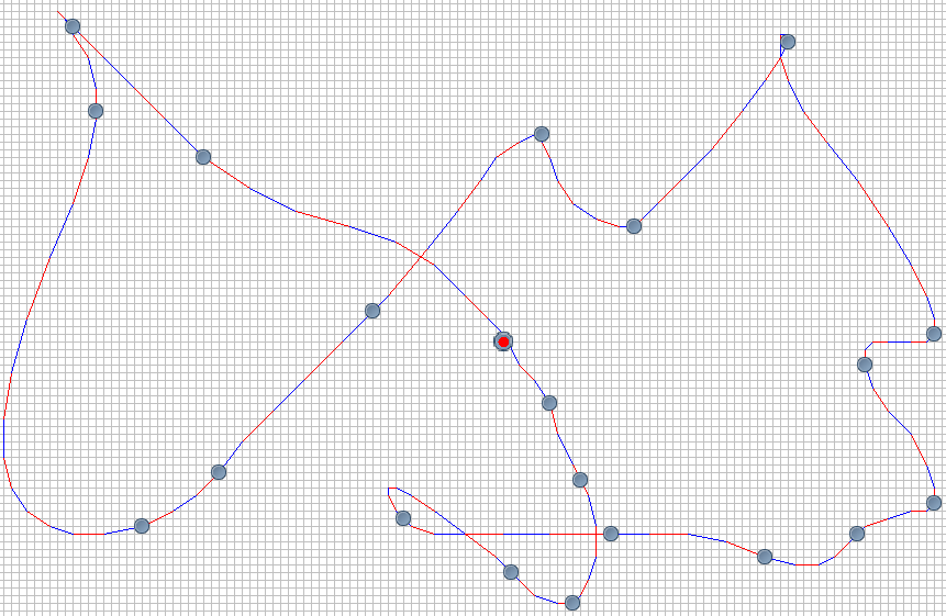
Figure 3: Example of a (possibly non-optimal) VTSP trajectory. The red point represents the starting city. The vectors of the trajectory are represented by alternating red/blue lines. (This trajectory is reversible and thus realizable in both directions.)

3 Preliminary results

In this section we make general observations about VectorTSP, some of which are used in the subsequent sections. In particular, we highlight those properties which are distinct from EuclideanTSP.

Fact 2.

The starting city has an impact on the cost of an optimal solution.

Example.

This can be observed on a small example, with $P=\{(0,0),(1,0),(2,0)\}$. Starting at $(0,0)$, a solution exists with $7$ configurations (i.e. 6 vectors), namely $T=(({(0,0),(0,0)}),$ $({(1,0),(1,0)}),$ $({(2,0),(1,0)}),$ $({(2,0),(0,0)}),$ $({(1,0),(-1,0)}),$ $({(0,0),(-1,0)}),$ $({(0,0),(0,0)}))$ (see the left picture). In contrast, if the tour starts at $(1,0)$, the vehicle will have to decelerate three times instead of two (right picture), which gives a trajectory of $8$ configurations ($7$ vectors).

Figure 4: Identical instances with distinct starting cities (shown in red) and corresponding optimal trajectories. For visibility, configurations are represented as arcs (or loops).

∎

This fact is the reason why an input instance of VectorTSP is also parameterized by a starting city $p_{0}\in P$. More generally, the cost of traveling between two given cities is impacted by the previous and subsequent positions of the vehicle and cannot be captured by a fixed cost, which is why VTSP does not straightforwardly reduce to classical TSP. The following fact strengthens the distinctive features of VTSP, showing that it does not straightforwardly reduce to ETSP either.

Lemma 1.

Let $\mathcal{I}$ be a VTSP instance on a set of cities $P$, in the default setting. Let $\pi$ be an optimal visit order for an ETSP instance on the same set of cities $P$, then racetrack($\pi$) may not be an optimal solution for $\mathcal{I}$.

Proof.

Consider the instance shown in Fig. 5. On the left, the trajectory corresponds to racetrack($\pi$), with $\pi$ an optimal visit order for the corresponding ETSP instance, starting and ending at $p_{0}$ (whence the final deceleration loop). In contrast, an optimal VTSP trajectory visiting the same cities (right picture) uses two less configurations, following a non-optimal visit order $\pi^{\prime}$ for ETSP. This lemma is also true if maximum visiting speed $\nu=0$ (see Fig. 6). ∎

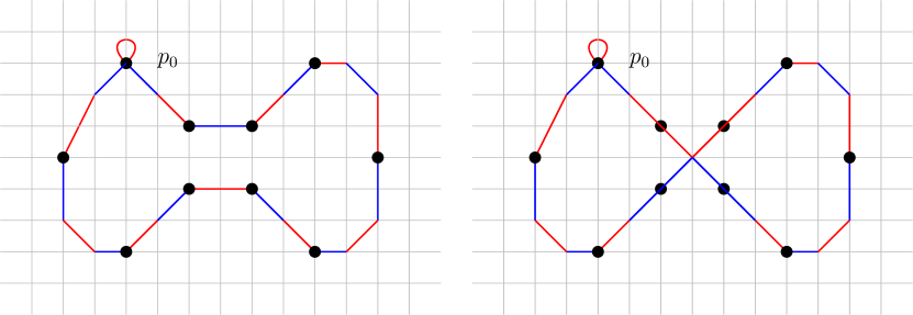
Figure 5: Trajectories of red and blue alternating vectors. racetrack($\pi$) (left picture, using 22 vectors) may not be an optimal solution (right picture, using 20 vectors, computed through a brute force algorithm).

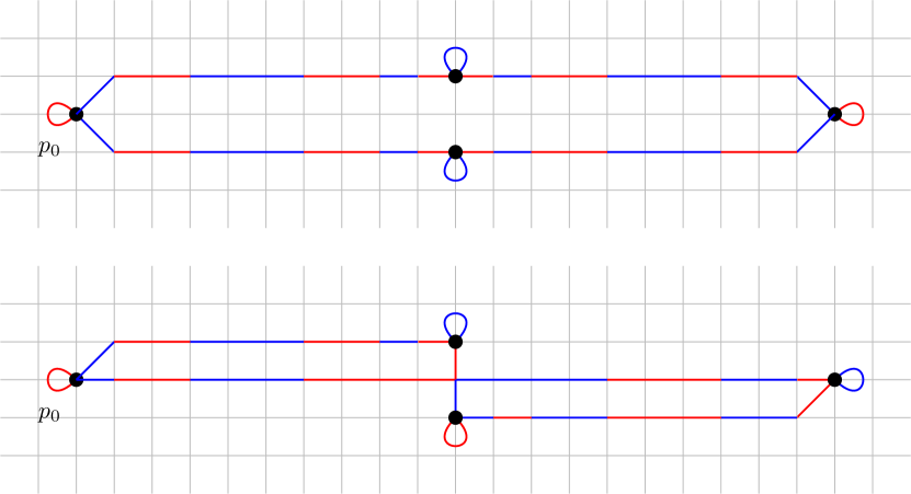
Figure 6: Trajectories of red and blue alternating vectors. racetrack($\pi$) (left picture, using 28 vectors) may not be an optimal solution (right picture, using 26 vectors, computed through a brute force algorithm), even if maximum visiting speed $\nu=0$.

Hence, solving VTSP does not reduce to optimizing the trajectory of an optimal ETSP solution: the visit order is impacted. This leads to the following interesting open question.

Open question 1.

Let $P$ be a set of cities. Let $\pi$ be an optimal tour for $P$ in the ETSP framework. Let $T_{OPT}$ be an optimal trajectory for $P$ in the context of VTSP (default setting). How different could the length of racetrack($\pi$) be from the length of $T_{OPT}$?

Furthermore, we observe the following two properties on Fig. 5 and Fig. 6 respectively, distinguishing VectorTSP even further from EuclideanTSP.

Fact 3.

An optimal VTSP solution may self-cross.

Fact 4.

The clockwise or counter-clockwise visit order may not be an optimal VTSP solution for cities placed on the vertices of a convex hull.

3.1 The configuration space can be bounded

The spirit of the racetrack model is to focus on acceleration only, without bounding the speed. Nonetheless, we show here that a trajectory in general (and an optimal one in particular) can always be found within a certain subgraph of the configuration graph, whose size is polynomially bounded in the size of the input. These results are formulated in the default setting for any discrete $d$-dimensional space.

Lemma 2 (Bounds on the solution length).

Let $P$ be a set of cities and $L$ be the largest distance in any dimension (over all $d$ dimensions) between two cities of $P$. Then a solution trajectory must contain at least $O(\sqrt{L})$ configurations. Furthermore, there always exists a solution trajectory of $O(L^{d})$ configurations.

Proof.

The lower bound follows from the fact that it takes at least $O(\sqrt{L})$ configurations to travel a distance of $L$ (starting at speed $0$), the latter being a lower bound on the total distance to be traveled. The upper bound can be obtained by exploring all the points of the $d$-dimensional rectangular hull containing the cities in $P$ at unit speed (with stops if visit speed $\nu=0$), which amounts to $O(L^{d})$ configurations. ∎

Lemma 3 (Bounds on the configuration graph).

An optimal trajectory for VTSP can be found in a subgraph of the configuration graph with polynomially many vertices and edges (in the size of the input), namely $O(L^{(2d^{2})})$.

Proof.

First observe that if there exists a trajectory of $O(L^{d})$ configurations, then this bound also applies to an optimal trajectory. Now, we know that a trajectory corresponds to a path in $G(\mathcal{C})$, thus an optimal trajectory can be found within the subgraph of $G(\mathcal{C})$ induced by the vertices at distance at most $O(L^{d})$ from the starting point. In $d$ dimensions, this amounts to $O((L^{d})^{2d})=O(L^{(2d^{2})})$ vertices. ∎

4 Computational complexity

Here, we present polynomial time reductions between VectorTSP and other NP-hard problems. More precisely, we establish NP-hardness of a particular parameterization of VectorTSP (and thus, of the general problem) where the visit speed $\nu$ is zero. The reduction is from ExactCover and is based on Papadimitriou’s proof to show NP-hardness of ETSP. In the other direction, we present a natural reduction from VectorTSP to GroupTSP. This reduction relies crucially on Lemma 3.

4.1 NP-hardness of VectorTSP

The proof goes through a number of intermediate steps before ending in the main theorem stating VectorTSP is NP-hard, being Theorem 4.2.

Let us first recall the definition of ExactCover. Let ${\cal U}$ be a set of $m$ elements (the universe), the problem ExactCover takes as input a set ${\cal F}=\{F_{i}\}$ of $n$ subsets of ${\cal U}$, and asks if there exists ${\cal F^{\prime}}\subseteq{\cal F}$ such that all sets in ${\cal F^{\prime}}$ are disjoint and ${\cal F^{\prime}}$ covers all the elements of ${\cal U}$. For example, if ${\cal U}=\{1,2,3\}$ and ${\cal F}=$ $\{\{1,2\},\{3\},\{2,3\}\}$, then ${\cal F}^{\prime}=\{\{1,2\},\{3\}\}$ is a valid solution, but $\{\{1,2\},\{2,3\}\}$ is not.

Given an instance $\cal I$ of ExactCover, the proof shows how to construct an instance $\cal I$’ of VTSP such that $\cal I$ admits a solution if and only if there is a trajectory visiting all the cities of $\cal I$’ using at most a certain number of configurations. We first give the high-level ideas of the proof, which are in common with that of Papadimitriou’s proof for ETSP. Then, we explain the details of the adaptation to VTSP.

The instance $\cal I^{\prime}$ is composed of several types of gadgets, representing respectively the subsets $F_{i}\in{\cal F}$ and the elements of ${\cal U}$ (with some repetition). For each $F_{i}$, a subset gadget $C_{i}$ is created which consists of a number of cities placed horizontally (wavy horizontal segments in Figure 7). For now, we state that each gadget can be traversed optimally in exactly two possible ways (without considering direction), which ultimately corresponds to including (traversal 1) or excluding (traversal 2) subset $F_{i}$ in the ExactCover solution. The $C_{i}$’s are located one below another, starting with $C_{1}$ at the top. Between every two consecutive gadgets $C_{i}$ and $C_{i+1}$, copies of element gadgets are placed for each element in ${\cal U}$, thus the element gadgets $H_{ij}$ are indexed by both $1\leq i\leq n-1$ and $1\leq j\leq m$ (see again Figure 7). The element gadgets are also made of a number of cities, whose particular organization is described later on. Finally, every subset gadget $C_{i}$ above or below an element gadget representing element $j$ is slightly modified in a way that represents whether $F_{i}$ contains element $j$ or not.

Intuitively, a tour visiting all the cities must choose between inclusion or exclusion of each $F_{i}$ (i.e., traversal 1 or 2 for each $C_{i}$). An element $j\in{\cal U}$ is considered as covered by a subset $F_{i}$ if $C_{i}$ does not visit any of the adjacent element gadgets representing $j$. Each element gadget $H_{i,j}$ must be visited either from above (from $C_{i}$) or from below (from $C_{i+1}$). Now, the number of subset gadgets is $n$, the number of element gadgets for each element is $n-1$ (one between every two consecutive subset gadgets), and the construction guarantees that at most one element gadget for each element $j\in{\cal U}$ is visited from a subset gadget $C_{i}$ (or the tour is non-optimal). These three properties collectively imply that for each element $j\in{\cal U}$, there is exactly one subset gadget $C_{i}$ that does not visit any of the element gadgets representing $j$.

Figure 7: Papadimitriou’s high-level construction

In summary, the tour proceeds from the top left corner through the $C_{i}$s (in order), visiting all the $H_{i,j}$. So long as a $C_{i}$ visits a $H_{i,j}$ (thus, from above), this means that element $j$ has not yet been covered in the ExactCover solution. Element $j$ is covered by subset $F_{i}$ in the ExactCover solution if $C_{i}$ is the subset gadget that does not visit the corresponding $H_{i,j}$, after which all the $H_{k\geq i,j}$ will necessarily be visited from below by the corresponding $C_{k+1}$, ensuring the element $j$ will not be covered more than once.

Setting the visiting speed $\nu=0$ is crucial for controlling the impact of acceleration, so as to force the optimal trajectory to follow the same pattern as in Papadimitriou’s proof. Section 4.1.1 specifies the corresponding intra-gadget spacing between cities and the spacing between the gadgets.

4.1.1 Technical aspects

This section describes in detail how to reduce an ExactCover instance to a VTSP instance with visit speed $\nu=0$. Our main modifications of Papadimitriou’s work are the careful repositioning and distancing of cities so as to force the trajectory to use an exact amount of vectors between some pairs of cities, and to avoid the trajectory being able to visit other cities than the desired visit order. For simplicity, it is first described in the $5$-successor model, i.e., the velocity can change only in one dimension at a time (Theorem 4.1). This constraint is subsequently relaxed to the default setting, including the $9$-successor model, resulting in Theorem 4.2.

The following definitions are from Papadimitriou [28]. A subset $P^{\prime}$ of the set of cities is an $a$-component if for all $p\in P^{\prime}$ we have $\texttt{min}(\texttt{cost}(p,p^{\prime}):p^{\prime}\not\in P^{\prime})\geq a$ and $\texttt{max}(\texttt{cost}(p,p^{\prime}):p^{\prime}\in P^{\prime})<a$, and $P^{\prime}$ is maximal w.r.t. these properties. A $k$-trajectory for a set of cities is a set of $k$, not closed trajectories visiting all cities. A valid trajectory for a VTSP instance is thus a closed (or cyclic) 1-trajectory. A subset of cities is $a$-compact if, for all positive integers $k$, an optimal $k$-trajectory has cost less than the cost of an optimal $(k+1)$-trajectory plus $a$. Note that $a$-components are trivially $a$-compact.

Lemma 4 (Papadimitriou [28]).

Suppose we have $N$ $a$-components $P_{1},...,P_{N}\in P$, such that the cost to connect any two components through a trajectory is at least $2a$, and $P_{0}$, the remaining part of $P$, is $a$-compact. Suppose that any optimal 1-trajectory of this instance does not contain any vectors between any two $a$-components. Let $K_{1},...,K_{N}$ be the costs of the optimal 1-trajectories of $P_{1},...,P_{N}$ and $K_{0}$ the cost of the optimal $(N+1)$-trajectory of $P_{0}$. If there is a 1-trajectory $T$ of $P$ consisting of the union of an optimal $(N+1)$-trajectory of $P_{0}$, $N$ optimal 1-trajectories of $P_{1},...,P_{N}$ and $2N$ trajectories of cost $a$ connecting $a$-components to $P_{0}$, then $T$ is optimal. If no such 1-trajectory exists, the optimal 1-trajectory of $P$ has a cost greater than $K=K_{0}+K_{1}+...+K_{N}+2Na$.

Consider the 1-chain structure presented in Figure 8. This structure is composed of cities positioned on a line, at distance one from one another. 1-chains can bend at 90 degrees angles, and only one optimal 1-trajectory exists, with a cost of $2(n-1)$ vectors for a 1-chain of length $n$.

(a)

(b)

(c)

Figure 8: 1-chain structure which turns $90^{\circ}$ twice. The distance between consecutive cities is 1. The optimal visit order is shown in $(b)$. We abbreaviate a 1-chain schematically as shown in $(c)$.

Next, consider the structure in Figure 9, referred to as a 2-chain. The distance between the leftmost (or rightmost) city and its nearby cities is $\sqrt{2}$. The closest distance between other cities is 2. The important thing to notice here is there exists only two distinct optimal 1-trajectories, denoted as mode 1 and mode 2, both of a cost of $3n+11$ for a 2-chain of length $n$.

(a)

(b)

(c)

(d)

Figure 9: 2-chain structure $(a)$. A 2-chain has precisely two optimal 1-trajectories, $(b)$ and $(c)$. We abbreviate a 2-chain schematically as shown in $(d)$.

(a)

(b)

(c)

Figure 10: Structure $H$. The distance between $A$ and $B$ is 2, between $A$ and $C$ 14, and between $A$ and $A^{\prime}$ 16. An optimal 1-trajectory in $H$ is shown in $(b)$. We abbreviate an $H$ structure schematically as shown in $(c)$.

Fact 5.

Among all 1-trajectories for $H$ (see Figure 10) having as endpoints two of the cities $A,A^{\prime},B,B^{\prime},C,C^{\prime},D,D^{\prime}$, there are 4 optimal 1-trajectories, namely those with endpoints $(A,A^{\prime})$, $(B,B^{\prime})$, $(C,C^{\prime})$, $(D,D^{\prime})$, which all have a cost of 77 vectors.

We are now ready to prove Theorem 4.1 using the above definitions, gadgets, and facts.

Theorem 4.1.

ExactCover reduces in polynomial time to VectorTSP with default setting, with maximum visiting speed $\nu=0$ and the $5$-successor model.

Proof.

The aforementioned structures are combined to construct a VTSP instance from a given ExactCover instance. Construct the structure shown in Figure 11, where $n$ is the number of subsets given in the corresponding ExactCover instance, and $m$ the number of elements in the universe.

Figure 11: Construction of the VTSP instance.

The 2-chains represent the subsets in ExactCover, and $H$ structures indirectly represent the elements in the universe. Finally, for every 2-chain $C_{i}$, replace the cities positioned directly above or below an $H$, by one of two structures, depending on the elements in $C_{i}$’s corresponding subset. If the subset contains the element corresponding to the above (or below) $H$, then replace by structure $A$ (see Figure 12), otherwise replace by structure $B$ (see Figure 13). The idea is to make it costly to visit an $H$ above or below from a structure $A$ traversed in mode 1.

(a)

(b)

(c)

Figure 12: Structure $A$ (see $(a)$). Visiting structure $A$ in mode 1 makes it costly to visit an $H$ structure above or below (see $(b)$). Visiting structure $A$ in mode 2 however, makes it less costly to visit an $H$ structure above (see $(c)$) or below.

(a)

(b)

(c)

Figure 13: Structure $B$ (see $(a)$). Visiting structure $B$ in any mode makes it advantageous to visit an $H$ structure above or below (see $(b)$ and $c$).

We observe that now the optimal cost to connect two $k$-paths between some 2-chain $C_{i}$ and some $H_{ij}$ (or $H_{(i-1)j}$) is 10 vectors, whereas the optimal cost to connect any two $k$-paths between two $H_{ij}$, is at least 40 vectors. Also, this optimal cost of 10 vectors between some 2-chain $C_{i}$ and some $H_{ij}$, can only be attained by a trajectory on a straight vertical line, thanks to the precise distance of 25. Deviating even the slightest bit from the vertical line would result in a non-optimal cost. The construction of the VTSP instance is now complete. It should be clear that an optimal 1-trajectory must have $Q$ and $R$ as endpoints. This construction meets the hypotheses of Lemma 4 with $a=10$, $N=m(n-1)$, $K_{1}=...=K_{N}=77$ and $K_{0}=1257mn+4m+557n+24p+1464$, where $p$ is the sum of cardinalities of all given subsets of the ExactCover instance. We examine when this structure has an optimal 1-trajectory $T$, as described in the lemma. $T$ traverses all 1-chains in the obvious way, and all 2-chains in one of the two traversals. Since its portion on $P_{0}$ has to be optimal, $T$ must visit a component $H$ from any configuration $B$ encountered, and it must return (by 5) to the symmetric city of $B$, since its portion on $H$ must be optimal, too. If $T$ encounters a configuration $A$ and the corresponding chain is traversed in traversal 2, $T$ will also visit a component $H$. However, if the corresponding chain is traversed in traversal 1, $T$ will traverse $A$ without visiting any configuration $H$, since all trajectories connecting $P_{0}$ and $H$ components must be of cost $a$. Moreover this must happen exactly once for each column of the structure, since there are $n-1$ copies of $H$ and $n$ structures $A$ or $B$ in each column. Hence, if we consider the fact that $C_{j}$ is traversed in traversal $1$ (resp. traversal $2$) to mean that the corresponding subset is (resp. is not) contained in the ExactCover solution, we see that the existence of a 1-trajectory $T$, as described in Lemma 4, implies the ExactCover instance admits a solution. Conversely, if the ExactCover instance admits a solution, we assign, as above, traversals to the chains according to whether or not the corresponding subset is included in the solution. It is then possible to exhibit a 1-trajectory $T$ meeting the requirements of Lemma 4. Hence the structure at hand has a 1-trajectory of cost no more than $K=1354mn-93m+557n+24p+1464$ if and only if the given instance of ExactCover is solvable. Finally, to obtain a valid VTSP trajectory, connect both endpoints $Q$ and $R$ in Fig. 11 with a 1-chain, and increase $K$ accordingly. ∎

Theorem 4.2.

ExactCover reduces in polynomial time to VectorTSP with default settings, except for maximum visiting speed $\nu=0$.

Proof.

The proof for the $9$-successor model is the same as for the $5$-successor model, except that the whole created VTSP instance $\cal I^{\prime}$ is tilted by $45\degree$ (the direction does not matter), and distances are scaled by $\sqrt{2}$. The value of $K$ is unchanged. This modification transposes the limitations of the $5$-successor model to the $9$-successor model. Indeed, due to the careful choice of distances involved, if one wishes to remain optimal while visiting the cities, one needs to only consider the outermost accelerations (diagonals) of the 9-successor version, as well as the null speed before turning (since different diagonals in the $9$-successor model cannot directly succeed one another). ∎

Note that a similar geometrical trick might be used to adapt the proof to further settings, such as continuous space with the continuous $d$-sphere successor function, such as depicted in Fig. 1 (for $\mathbb{R}^{2}$). Also, intuitively, one may simply remove the null vectors, so as to consider a maximum visiting speed $\nu=1$.

4.2 Transformation from VectorTSP to GroupTSP

Here, we show that VTSP reduces in polynomial time to GroupTSP (also known as SetTSP or GeneralizedTSP), where the input is a set of cities partitioned into groups, and the goal is to visit at least one city in each group.

Lemma 5.

VectorTSP admits a natural polynomial-time reduction to GroupTSP.

Proof.

Let $\cal I$ be the VTSP instance and $n$ the number of cities in $\cal I$. Each city in $\cal I$ can be visited in a number of different ways, each corresponding to a different configuration in ${\cal C}$ (the set of all possible configurations). The strategy is to create a city in $\cal I$’ for each configuration that visits at least one city in $\cal I$, and group them according to which city of $\cal I$ they visit (the other configurations are discarded). Thus, visiting a city in each group of $\cal I$’ corresponds to visiting all cities in $\cal I$. Depending on the parameters of the model (visit speed, visit distance, vector completion), it may happen that a same configuration visits several cities in $\cal I$, which implies that the groups may overlap; however, Noon and Bean show in [24] that a GTSP instance with overlapping groups can be transformed into one with mutually exclusive groups at the cost of creating $k$ copies of a city when it appears originally in $k$ different groups. Thus we proceed without worrying about overlaps. Let $X$ be the set of cities in $\cal I$, and ${\cal C}(x)\subseteq{\cal C}$ be the configurations which visit city $x\in X$. Instance $\cal I$’ is defined by creating a city for each configuration in $\cup_{x\in X}{\cal C}(x)$ and a group for each ${\cal C}(x)$. An arc is added between all couples $(c_{1},c_{2})$ of cities in $\cal I$’ such that $c_{1}$ and $c_{2}$ belong to different groups; the weight of this arc is the distance between $c_{1}$ and $c_{2}$ in the configuration graph. Thus, a trajectory using $k$ configurations to visit all the cities in $\cal I$ corresponds to a tour of cost $k$ visiting at least one city in each group in $\cal I$’. The fact that the reduction is polynomial (both in time and space) results from the facts that (1) there is a polynomial number of relevant configurations (Lemma 3), each one being copied at most $n$ times; and (2) the distance between two configurations in the configuration graph can be computed in polynomial time (1). ∎

Note that this reduction is general in terms of the parameters: any combination $\nu$, $\alpha$, and $\beta$ only impacts the set of vectors that visit each city. Lemma 5 implies the following corollary.

Corollary 1 (Through [24]).

VectorTSP admits a natural polynomial-time reduction to AsymmetricTSP.

Indeed, Noon and Bean [24] present a polynomial time reduction from GTSP to ATSP. This is done by adding arcs of cost zero inside every group, creating a cycle visiting all nodes in the group. Suppose w.l.o.g. the created cycle $x_{1},x_{2},...,x_{k},x_{1}$, then for all arcs $(x_{i},y_{j})$, with $y_{j}$ some node in another group, replace by arcs $(x_{i-1},y_{j})$. Outgoing arcs of node $x_{1}$ get replaced on node $x_{k}$. This effectively shifts all outgoing arcs in each group, such that an optimal tour is forced to visit all nodes in a group before visiting another. Unfortunately, the resulting ATSP instance does not respect triangular inequality, which prevents us from approximating it using techniques from [33]. In turn, we have the following corollary.

Corollary 2 (Through [18]).

VectorTSP admits a natural polynomial-time reduction to SymmetricTSP.

Kanellakis and Papadimitriou proved any AsymmetricTSP instance such as we can obtain in Corollary 1, can be reduced into a SymmetricTSP instance. The main idea is to simulate an ATSP as follows. Add three nodes $i_{1}$, $i_{2}$ and $i_{3}$ for every node $i$ in the ATSP. Add (undirected) edges $(i_{1},i_{2})$ and $(i_{2},i_{3})$ of cost 0 to $i_{2}$. Add (undirected) edges $(i_{3},j_{1})$ if $(i,j)\in E$ of the ATSP, with the same cost. This reduction triples the amount of nodes of the instance. This was later improved to only double the amount of nodes, first by Jonker and Volgenant [17] and later by Kumar and Li [21].

5 Algorithms

In this section, we present an algorithmic framework for finding acceptable solutions to VTSP in practical polynomial time. It is based on an interaction between a high-level part that decides the visit order, and a trajectory oracle that evaluates its cost.

5.1 Exploring visit orders (FlipVTSP)

A classical heuristic for ETSP is the so-called 2-opt algorithm [10], also known as Flip. It is a local search algorithm which starts with an arbitrary tour $\pi$. In each step, all the possible flips, i.e. inversions of suborders, of the current tour $\pi$ are evaluated. If such a flip $\pi^{\prime}$ improves upon $\pi$, it is selected and the algorithm recurses on $\pi^{\prime}$. Eventually, the algorithm finds a local optimum whose quality is commonly admitted to be of reasonable quality, albeit without guarantees (the name 2-opt does not reflect an approximation ratio, it stands for 2-permutation local optimality). Adapting this algorithm seems like a natural option for the high-level part of our framework.

The main differences between our algorithm, called FlipVTSP, and its ETSP analogue are that (1) the cost of a tour is not evaluated in terms of distance, but in terms of the required number of racetrack configurations (through calls to the oracle); and (2) the number of recursions is polynomially bounded because new tours are considered only in case of improvement, and the length of a trajectory is itself polynomially bounded (Lemma 2). The resulting tour is a local optimum with respect to flips, also known as a 2-optimal tour. For completeness, the algorithm is given by Algorithm 1.

Algorithm 1 : 2-opt.

Input: a set $P$ of cities.
Output: a $2$-optimal tour w.r.t. the racetrack model.

1:$\pi_{opt}\leftarrow\texttt{init}(P)$

2:$C_{opt}\leftarrow\texttt{oracle(}\pi_{opt}\texttt{)}$

3:$improved\leftarrow\texttt{true}$

4:while $improved$ do

5:     $improved\leftarrow\texttt{false}$

6:     for each city $i$ (except starting city) do

7:         for each other city $j$ (except starting city) do

8:              $\pi_{test}\leftarrow\texttt{flip(}\pi_{opt},i,j\texttt{)}$

9:              $C_{test}\leftarrow\texttt{oracle(}\pi_{test}\texttt{)}$

10:              if $C_{test}<C_{opt}$ then

11:                  $\pi_{opt}\leftarrow\pi_{test}$

12:                  $C_{opt}\leftarrow C_{test}$

13:                  $improved\leftarrow\texttt{true}$

14:                  break                          

15:         if $improved$ then

16:              break                  

17:return $\pi_{opt}$

Theorem 5.1.

One can find a 2-optimal tour for VTSP in time $O(n^{2}L^{d}\tau(n,L))$, where $n$ is the number of cities, $L$ the largest distance between two cities in a dimension, $d$ the number of dimensions, and $\tau(n,L)$ the time complexity of the oracle for computing the cost of an optimal trajectory for a given visit order.

Proof.

As explained in (the proof of) Lemma 2, if the visit order is not imposed, then one can easily find a trajectory of length $O(L^{d})$ that visits all the cities, through walking over the entire area (rectangle hull containing the cities). Let $\pi$ be the order in which the cities are visited by such a walk. This visit order is the one returned by the init() function. Then $C_{opt}$ is accordingly initialized with cost $O(L^{d})$ in line 2. Now, the main loop iterates only if a shorter trajectory is found, which can occur at most as many times as the length of the initial trajectory. Then, in each iteration, up to $O(n^{2})$ flips are evaluated, with a nested call to the oracle. ∎

5.2 Optimal trajectory for a visit order (Multipoint $A^{*}$)

Here, we discuss the problem of computing an optimal trajectory that visits a set of points in a given order. A previous work of interest is Bekos et al. [5], which addresses the problem of computing an optimal Racetrack trajectory in the so-called “Indianapolis” track, where the track has a fixed width and right-angle turns. This particular setting limits the maximum speed at the turns, which makes it possible to decompose the computation in a dynamic programming fashion. In contrast, the space is open in VTSP, with no simple way to bound the maximum speed. Therefore, we propose a different strategy based on searching for an optimal path in the configuration graph using $A^{*}$.

The problem: Given an ordered sequence of points $\pi=(p_{1},p_{2},\dots,p_{n})$, compute (the cost of) an optimal trajectory realizing $\pi$, i.e., visiting the points in order, starting at $p_{1}$ and ending at $p_{n}$ at zero speed. (In the particular case of VTSP, $p_{1}$ and $p_{n}$ coincide.)

Finding the optimal trajectory between two configurations already suggests the use of path-finding algorithms like BFS, Dijkstra, or $A^{*}$ (see e.g. [32] and [5]). The difficulty in our case is to force the path to visit all the intermediary points in order. Our contribution here is to design an estimation function that guides $A^{*}$ through these constraints. In general, $A^{*}$ explores the search space by generating a set of successors of the current node (in our case, configuration) and estimating the remaining cost of each successor using a problem-specific function. The successors are then inserted into a data structure (in general, a priority queue) which makes it easy to continue exploration from the position which is currently the best estimated. The great feature of $A^{*}$ is that it is guaranteed to find an optimal path, provided that the estimation function does not over-estimate the actual cost, and so, is as fast as the estimation is precise (whereas no estimation function basically reduces $A^{*}$ to Dijkstra’s algorithm).

5.2.1 Cost estimation function

For simplicity, we first present how the estimation works relative to the entire tour. Then we explain how to generalize it for estimating an arbitrary intermediate configuration in the trajectory (i.e. one that has already visited a certain number of cities and is located at a given position with given velocity). The key insight is that the optimal trajectory, whatever it be, must obey some pattern in each dimension. Consider, for example, the tour $\pi=((5,10),(10,12),(14,7),(8,1),(3,5),(5,10))$ shown on Figure 14. In the $x$-dimension, the vehicle must move at least from $1$ to $3$, then stop at a turning point, change direction, and travel towards $5$, then stop and change direction again, and travel back to $1$. Thus, any trajectory realizing $\pi$ can be divided into three subtrajectories, whose cost is at least the cost of traveling along these segments in the $x$-dimension, starting and ending at speed 0 at the turning points. Thus, in the above example, the vehicle must travel at least along distances $9$, $11$, and $2$ (with zero speed at the endpoints), which gives a cost of at least $16$ (i.e., 6, 7, and 3 respectively). The details of these computations are given in Section 5.2.2. The same analysis can be performed in each dimension; then, the actual cost must be at least the maximum value among these costs, which is therefore the value we consider as estimation.

Figure 14: Projection in dimensions $x$ and $y$, with corresponding one-dimensional trajectories of lengths $16$ and $17$ respectively. The estimated cost for this tour is thus $17$.

In general, the configurations whose estimation is required by $A^{*}$ are more general than the above case. In particular, it can have an arbitrary position and velocity, and the vehicle may have already visited a number of cities. Therefore, the estimated cost is evaluated according to the remaining sub-tour. The only technical difference is that one must take into account the current position and velocity when determining where the next turning point is in the dimensional projection, which poses no significant difficulty. Concretely, a case-based study of the initial configuration with respect to the first turning point, allows one to self-reduce the estimation to the particular case that the initial speed is zero (possibly at a different position). The overall unidimensional cost amounts to the sum of costs between such consecutive pairs, whose individual values can be computed in constant time by a closed formula (Lemma 7 in Section 5.2.2).

Lemma 6.

The cost estimation of a subtour $\pi^{\prime}=c,p_{i},...,p_{n}$, where $c$ is the current configuration and $p_{i},\ldots,p_{n}$ is a suffix of $\pi$ can be computed in $O(n)$ time.

Proof.

As explained, the subtour is first reduced to a subtour $\pi^{\prime\prime}=p_{i-1},p_{i},\ldots,p_{n}$. The turning points in $\pi^{\prime\prime}$ are easily identified through a pass over $\pi^{\prime\prime}$. Their number is at most $n$ because they are a subset of the points in $\pi^{\prime\prime}$. Finally, the cost between each pair of selected turning points can be computed in constant time (Lemma 7). ∎

We can now conclude regarding the time complexity of the multipoint $A^{*}$ algorithm.

Theorem 5.2.

The multipoint $A^{*}$ algorithm runs in polynomial time, more precisely in time $\widetilde{O}(L^{(2d^{2})}n^{2})$.

Proof.

A “configuration” of the $A^{*}$ algorithm (let us call it a state, to avoid ambiguity) is made of a configuration $c$ together with a number $k$ of visited cities. There are at most $O(L^{(2d^{2})})$ configurations (Lemma 3) and $n$ cities, thus $A^{*}$ will perform at most $O(L^{(2d^{2})}n)$ iterations, provided that it does not explore a state twice. Given that the states are easily orderable, the later condition can be enforced by storing all the visited states in an ordered collection that is searchable and insertable in logarithmic time (whence the $\widetilde{O}$ notation). Finally, for each state an estimated remaining cost can be computed in $O(n)$ time (Lemma 6). ∎

The combined use of FlipVTSP and Multipoint $A^{*}$ thus runs in polynomial time (Theorem 5.1 and 5.2).

5.2.2 Unidimensional cost estimation

We present here efficient computations of optimal costs (number of vectors) between two unidimensional coordinates spaced by $d$ units, first when the initial and final speed are both zero, and afterwards when the final speed is zero and the initial speed is arbitrary.

Lemma 7.

In a single dimension, the cost to cover $d$ space units with initial and final speed $dx=0$ is $\lceil 2\sqrt{d}\rceil$.

Proof.

For the special case that $d=0$, the formula gives a cost of $0$, which is trivially correct. For $d>0$, let us consider independently a set of accelerating vectors in the first half of the segment of length $d$, and a symmetrical set of decelerating vectors in the second half, such as shown in Figure 15. Let $s$ be the length of the largest vector used before the middle point is reached (in Fig. 15, $s=3$). This corresponds also to the number of accelerating vectors, since the length of these vectors increases in each step by one unit. The distance covered by these vectors is thus of $s(s+1)/2$, and same for the decelerating vectors, which gives a total of $s(s+1)$ units. In the middle of the segment, these vectors may or may not align exactly, the three possible cases are as follows:

1. If $d=s(s+1)$, i.e. the accelerating and decelerating vectors align perfectly in the middle, then no extra vector is needed apart from the last selfloop at the arrival (for reaching zero speed), which gives a total cost of $2s+1$ vectors. Furthermore, since $s^{2}<d<(s+0.5)^{2}$, this cost amounts to $\lceil 2\sqrt{d}\rceil$ vectors.

2. If $s(s+1)<d\leq(s+1)^{2}$, then $s^{2}+s+1\leq d\leq s^{2}+2s+1$ (since $d$ is an integer). In this case, there is a non-empty space in the middle and a trajectory of $2s+1$ vectors (including the final loop) can clearly not exist. Let $d^{\prime}\leq s+1$ be the size of this space ($d^{\prime}=1$ in Fig. 15) . One can complete the trajectory by adding a single vector of length $d^{\prime}$. If $d\geq s-1$, this vector may be added in the middle. If $d^{\prime}<s-1$, then a vector of length $d^{\prime}$ already exists in the accelerating vectors. It suffices to repeat this vector once and shift the subsequent ones (dashed green vector in Fig. 15) in order to obtain a complete trajectory of $2s+2$ vectors. Finally, since $(s+0.5)^{2}<d\leq(s+1)^{2}$, this cost amounts again to $\lceil 2\sqrt{d}\rceil$.

3. If $(s+1)^{2}<d<(s+1)(s+2)$, then $s^{2}+2s+2\leq d\leq s^{2}+3s+1$ (since $d$ is an integer). In this case, the vectors leave an uncovered space of $d^{\prime}$ units, with $s+2\leq d^{\prime}\leq 2s+1$. No trajectory with $2s+2$ vectors (including the loop) exist, since $d^{\prime}$ exceeds the size allowed for an additional vector. However, one can complete the trajectory by splitting $d^{\prime}$ in a sum of two numbers $\leq s+1$ and duplicate the corresponding vectors in (say) the accelerating segment. Since $(s+1)^{2}<d\leq(s+1.5)^{2}$, this amounts to $2s+3=\lceil 2\sqrt{d}\rceil$ vectors in total.

To conclude, note that the case that $d\geq(s+1)(s+2)$ never occurs, as otherwise an additional vector of length $s+1$ could have been added in the setup phase, to both the accelerating and decelerating sequences.

$\downarrow$

Figure 15: Computation of an optimal 1D trajectory for $d=13$. Vectors are represented by arcs for visibility.

∎

We remark that the sequence of integers produced by the formula $\lceil 2\sqrt{d}\rceil$ corresponds to sequence A027434 in the On-line Encyclopedia of Integer Sequences [1]. For completeness, we now address, as a corollary, the case that the initial speed is non-zero (this case is also used in the algorithm).

Corollary 3.

In a single dimension, the cost from some position $x$ with initial speed $dx$, to some position $p$ with final speed zero, can be computed in constant time.

Proof.

Considering different speeds does not add significant difficulty. Indeed, all cases can be reduced to a case with speed $dx=0$ (treated in Lemma 7). If $dx<0$, slow down to zero speed, add the necessary amount of vectors to do so, $-dx$, to the cost, and next compute the cost from $x^{\prime}=x-\frac{dx(dx+1)}{2}$ to $p$ with velocity $dx=0$. If $dx>0$ and very large (large enough to bypass $p$, even when continuously decelerating), then also slow down to zero speed. Now, concerning the context of our multipoint $A^{*}$ algorithm, if $p$ is a turning point’s projection, consider the next turning point’s (or final city’s) projection $p^{\prime}$ and next compute the cost from $x^{\prime}=x+\frac{dx(dx-1)}{2}$ to $p^{\prime}$ with velocity $dx=0$. If however $p$ is the final city’s projection, next compute the cost from $x^{\prime}$ to $p$ with velocity $dx=0$. Lastly, if $dx>0$, but not so large as to bypass $p$ by only decelerating, add $-dx$ to the cost, and compute the cost from $x^{\prime}=x-\frac{dx(dx+1)}{2}$ to $p$ with velocity $dx=0$. ∎

5.3 A faster heuristic using limited views.

Our presented multipoint $A^{*}$ algorithm always finds the optimum, but in practice, it only scales up to medium-sized instances (see Section 6). If one is willing to lose some precision, then a simple trick (also used in [5]) can be used to scale with the number of cities. The idea is to compute limited sequential sections of the trajectory and glue them together subsequently. Concretely, given a tour $\pi=p_{1},...,p_{n}$, the limited view heuristic runs multipoint $A^{*}$ on a sliding window of fixed length $l$ (typically 5 or 6 cities) over $\pi$. For each offset $i$ of the window, the trajectory is computed from $p_{i}$ to $p_{i+l}$ ($p_{n}$, if less than $l$ cities remain). Then, of the computed trajectory, only the subtrajectory $T_{i}$ from $p_{i}$ to $p_{i+1}$ is retained, the offset advances to $i+1$ and multipoint $A^{*}$ is run again, using the last configuration of $T_{i}$ as initial configuration. Finally, the algorithm returns the concatenation of the $T_{i}$s.

6 Experiments and conclusion

In this section, we present a few experiments with the goal to (1) validate the algorithmic framework described in Section 5, and (2) motivate the VTSP problem itself, by quantifying the discrepancy between ETSP and VTSP. The instances were generated by distributing cities uniformly at random within a given square area. For each instance, TSP solver Concorde [2] was used to obtain the reference optimal ETSP tour $\pi$. The optimal trajectory $T=\texttt{racetrack($\pi$)}$ realizing this tour was computed using Multipoint $A^{*}$ (with complete view). Then, FlipVTSP explored the possible flips (with limited view) until a local optimum is found. An example is shown on Figure 16 (right), resulting from $2$ flips on $T=\texttt{racetrack($\pi$)}$ (left). Finding these flips is left as an exercise.

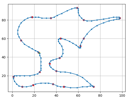
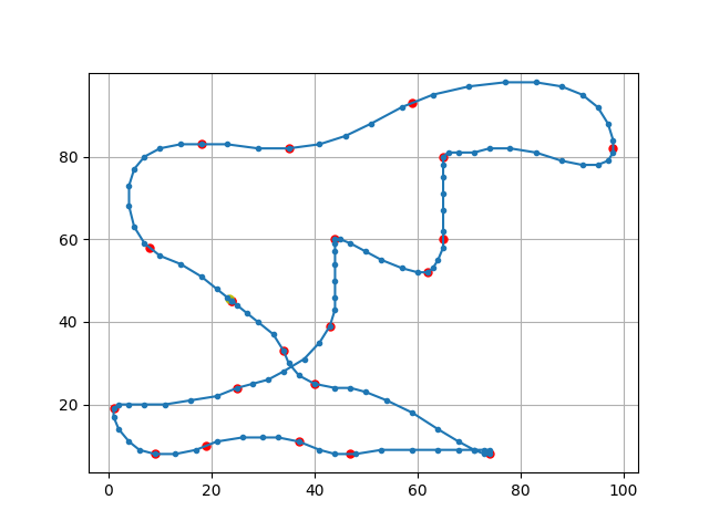
Figure 16: Example of tour improvement (128 vectors vs. 120 vectors).

Such an outcome is not rare. Figs. 17, LABEL:, 18, LABEL: and 19 show some measures when varying (1) the number of cities in a fixed area; (2) the size of the area for a fixed number of cities; and (3) both at constant density. The plots show the likelihood of at least one improving flip happening, as well as the average number of flips, tested on $100$ random instances. For performance, only the flips which did not deteriorate the EuclideanTSP tour distance by too much were considered (15 %, empirically). Thus, the plots tend to under-estimate the impact of VTSP (they already do so, by considering only local optima, and limited view in the flip phase).

The results suggest that an optimal ETSP visit order becomes less likely to be optimal for VTSP as the number of cities increases. The size of the area for a fixed number of cities does not seem to have a significant impact. Somewhat logically, scaling both parameters simultaneously (at constant density) seems to favor VTSP as well. Further experiments should be performed for a finer understanding. However, these results are sufficient to confirm that VTSP is a specific problem.

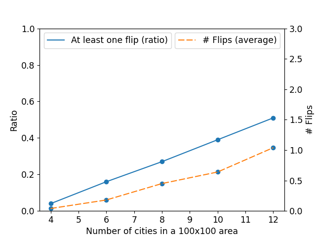
Figure 17: Varying the number of cities within a fixed $100\times 100$ area.

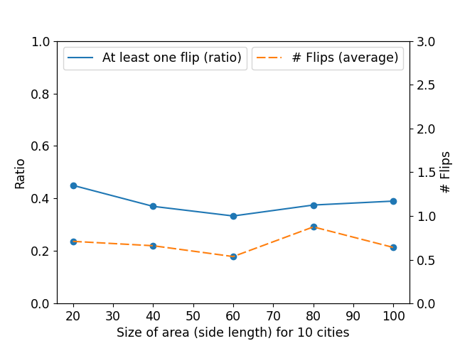
Figure 18: Varying the size of the area, considering 10 cities.

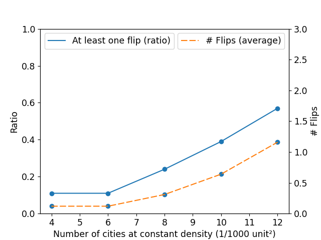
Figure 19: Varying the number of cities and the size of the area, but keeping constant density of $1$ city per $1000$ unit².

References

- [1] A027434, S.: On-line encyclopedia of integer sequences https://oeis.org/A027434
- [2] Applegate, D., Bixby, R., Chvatal, V., Cook, W.: Concorde tsp solver (2006)
- [3] Arkin, E.M., Hassin, R.: Approximation algorithms for the geometric covering salesman problem. Discrete Applied Mathematics 55(3), 197–218 (1994)
- [4] Arora, S.: Polynomial time approximation schemes for euclidean tsp and other geometric problems. In: Proceedings of 37th Conference on Foundations of Computer Science. pp. 2–11. IEEE (1996)
- [5] Bekos, M.A., Bruckdorfer, T., Förster, H., Kaufmann, M., Poschenrieder, S., Stüber, T.: Algorithms and insights for racetrack. Theoretical Computer Science (2018)
- [6] Bjorklund, A.: Determinant sums for undirected hamiltonicity. SIAM Journal on Computing 43(1), 280–299 (2014)
- [7] Canny, J., Donald, B., Reif, J., Xavier, P.: On the complexity of kinodynamic planning. IEEE (1988)
- [8] Canny, J., Rege, A., Reif, J.: An exact algorithm for kinodynamic planning in the plane. Discrete & Computational Geometry 6(3), 461–484 (1991)
- [9] Christofides, N.: Worst-case analysis of a new heuristic for the travelling salesman problem. Tech. rep., Carnegie-Mellon Univ Pittsburgh Pa Management Sciences Research Group (1976)
- [10] Croes, G.A.: A method for solving traveling-salesman problems. Operations research 6(6), 791–812 (1958)
- [11] Donald, B., Xavier, P., Canny, J., Reif, J.: Kinodynamic motion planning. Journal of the ACM (JACM) 40(5), 1048–1066 (1993)
- [12] Erickson, J.: Ernie’s 3d pancakes : ”how hard is optimal racing?” (2009), http://3dpancakes.typepad.com/ernie/2009/06/how-hard-is-optimal-racing.html
- [13] Gardner, M.: Sim, chomp and race track-new games for intellect (and not for lady luck). Scientific American 228(1), 108–115 (1973)
- [14] Garey, M.R., Graham, R.L., Johnson, D.S.: Some np-complete geometric problems pp. 10–22 (1976)
- [15] Held, M., Karp, R.M.: A dynamic programming approach to sequencing problems. Journal of the Society for Industrial and Applied mathematics 10(1), 196–210 (1962)
- [16] Holzer, M., McKenzie, P.: The computational complexity of racetrack pp. 260–271 (2010)
- [17] Jonker, R., Volgenant, T.: Transforming asymmetric into symmetric traveling salesman problems. Operations Research Letters 2(4), 161–163 (1983)
- [18] Kanellakis, P.C., Papadimitriou, C.H.: Local search for the asymmetric traveling salesman problem. Operations Research 28(5), 1086–1099 (1980)
- [19] Karlin, A.R., Klein, N., Gharan, S.O.: A (slightly) improved approximation algorithm for metric tsp. In: Proceedings of the 53rd Annual ACM SIGACT Symposium on Theory of Computing. pp. 32–45 (2021)
- [20] Karp, R.M.: Reducibility among combinatorial problems pp. 85–103 (1972)
- [21] Kumar, R., Li, H.: On asymmetric tsp: Transformation to symmetric tsp and performance bound. Journal of Operations Research 6 (1996)
- [22] Le Ny, J., Frazzoli, E., Feron, E.: The curvature-constrained traveling salesman problem for high point densities. In: 2007 46th IEEE Conference on Decision and Control. pp. 5985–5990. IEEE (2007)
- [23] Mitchell, J.S.: Guillotine subdivisions approximate polygonal subdivisions: A simple polynomial-time approximation scheme for geometric tsp, k-mst, and related problems. SIAM Journal on computing 28(4), 1298–1309 (1999)
- [24] Noon, C.E., Bean, J.C.: An efficient transformation of the generalized traveling salesman problem. INFOR: Information Systems and Operational Research 31(1), 39–44 (1993)
- [25] Olsson, R., Tarandi, A.: A genetic algorithm in the game racetrack (2011)
- [26] Orponen, P., Mannila, H.: On approximation preserving reductions: Complete problems and robust measures (revised version). Department of Computer Science, University of Helsinki (1990)
- [27] Papadimitriou, C., Vempala†, S.: On the approximability of the traveling salesman problem. Conference Proceedings of the Annual ACM Symposium on Theory of Computing 26, 101–120 (02 2006). https://doi.org/10.1007/s00493-006-0008-z
- [28] Papadimitriou, C.H.: The euclidean travelling salesman problem is np-complete. Theoretical computer science 4(3), 237–244 (1977)
- [29] Preparata, F.P., Shamos, M.I.: Computational geometry: an introduction. Springer Science & Business Media (2012)
- [30] Savla, K., Bullo, F., Frazzoli, E.: Traveling salesperson problems for a double integrator. IEEE Transactions on Automatic Control 54(4), 788–793 (2009)
- [31] Savla, K., Frazzoli, E., Bullo, F.: On the point-to-point and traveling salesperson problems for dubins’ vehicle. In: proceedings of the American Control Conference. vol. 2, p. 786 (2005)
- [32] Schmid, J.: Vectorrace - finding the fastest path through a two-dimensional track. URL: http://schmid.dk/articles/vectorRace.pdf (2005)
- [33] Svensson, O., Tarnawski, J., Végh, L.A.: A constant-factor approximation algorithm for the asymmetric traveling salesman problem. In: Proceedings of the 50th Annual ACM SIGACT Symposium on Theory of Computing. pp. 204–213. ACM (2018)
- [34] Yuan, Y., Peng, Y.: Racetrack: An approximation algorithm for the mobile sink routing problem. In: Nikolaidis, I., Wu, K. (eds.) Ad-Hoc, Mobile and Wireless Networks. pp. 135–148. Springer Berlin Heidelberg, Berlin, Heidelberg (2010)