Near- and mid-infrared observations in the inner tenth of a parsec of the Galactic center
Detection of proper motion of a filament very close to Sgr A*

Abstract

We analyze the gas and dust emission in the immediate vicinity of the supermassive black hole Sgr A* at the Galactic center (GC) with the ESO VLT (Paranal/Chile) instruments SINFONI and VISIR. The SINFONI H+K data cubes show several emission lines with related line map counterparts. From these lines, the Br$\gamma$ emission is the most prominent one and appears to be shaped as a bar extending along the North-South direction. With VISIR, we find a dusty counterpart to this filamentary emission. In this work, we present evidence that this feature can be most likely connected to the mini-spiral and potentially influenced by the winds of the massive stars in the central cluster or an accretion wind from Sgr A*. To this end, we co-add the SINFONI data between 2005 and 2015. The spectroscopic analysis reveals a range of Doppler-shifted emission lines. We also detect substructures in the shape of clumps that can be investigated in the channel maps of the Br$\gamma$-bar. In addition, we compare the detection of the near-infrared (NIR) Br$\gamma$ feature to PAH1 mid-infrared (MIR) observations and published 226 GHz radio data. These clumps show a proper motion of about $320$km/s that are consistent with other infrared continuum detected filaments in the Galactic center. Deriving a mass of $2.5\,\times\,10^{-5}\,M_{\odot}$ for the investigated Br$\gamma$-feature shows an agreement with former derived masses for similar objects. Besides the North-South Br$\gamma$-bar, we find a comparable additional East-West feature. Also, we identify several gas reservoirs that are located west of Sgr A* that may harbor dusty objects.

1 Introduction

Investigating the vicinity of supermassive black holes (SMBHs), and in particular the vicinity of the SMBH associated with the compact radio source Sgr A*, is often connected to the investigation of gas and dust on large ($>>$ 1 pc) and small scales ($<$ 1 pc ). This is important if one wants to characterize star formation or to determine the mass of the SMBH itself. In this context, Wollman et al. (1977) used the mini-spiral gas velocities to derive the Sgr A* SMBH mass. Yusef-Zadeh et al. (1998) and Zhao & Goss (1998) also observed proper motions of gaseous-dusty structures and filaments based on their radio continuum detections in the vicinity of Sgr A* and the Galactic Center (GC) stellar association IRS13E. Mužić et al. (2007) completed that picture by expanding the analysis towards shorter wavelengths in the near-infrared (NIR). These publications derive typical gas and dust filament velocities of several hundred km/s.

However, extragalactic studies of gas and dust on larger scales by Böker et al. (2008) lead to the introduction of two models that could describe the feeding process of SMBHs as well as the provision of a gas reservoir which is responsible for star formation – “popcorn model” and “pearls on a string” scenarios. A large amount of the dusty and gaseous material typically accumulates along the ring on the scale of 100 parsecs and less at the innermost dynamical resonance referred to as the inner or nuclear Lindblad resonance (Fukuda et al., 1998). Böker et al. (2008) discuss two scenarios of star-formation along the nuclear ring. The “popcorn model” describes a scenario when the gas is accumulated along the ring rather uniformly so that the critical density is reached throughout the whole ring. As a result, there is no age gradient of star-forming clusters along the ring. The “pearls on a string” model operates with the localized burst of star-formation in so-called overdensity regions, which can often be associated with the sites where the gas material enters the ring. The star-forming clusters are then formed along the ring in a sequential way which leads to the age gradient. The “pearls on a string” scenario is supported by observational data (Böker et al., 2008; Fazeli et al., 2019).

For the Galactic center, Nayakshin et al. (2007) and Jalali et al. (2014) modeled the gravitational influence of the SMBH on molecular clouds on intermediate scales that are moving from a distance of several parsecs towards Sgr A*. The authors find indications that in-falling material could trigger star formation in the close vicinity of the SMBH. On larger scales, this could be linked to the proposed ”Pearls on a string” model. It is evident, that the investigation of gas and dust reservoirs located in the inner and outer parsecs contributes to the understanding of star formation (Böker et al., 2008; Jalali et al., 2014) and black hole feeding.

A key question is how the material is transported from the larger scales all the way to Sgr A*. An occasional collision of clumps inside the circumnuclear disk (CND), which is located between $1.5$ to $7$ pc, can lead to the loss of angular momentum and the formation of streamers that are tidally interacting with the SMBH – the Minispiral streamers can be the manifestation of this process (Jalali et al., 2014). Another way to fill the central cavity inside the CND is the interaction of stellar winds with the inner rim of the CND, which can also lead to the formation of infalling denser clumps that are tidally interacting with Sgr A* (Blank et al., 2016). Finally, thermal instability could have operated in the central parsec during the phases of enhanced activity of Sgr A*, which would create a multiphase medium where the warm and more diluted plasma material is in approximate pressure equilibrium with the colder and denser gas (Różańska et al., 2014, 2017).

In this work, we investigate the Br$\gamma$ gas reservoir in the direct vicinity of Sgr A*, the SMBH of our host Galaxy. We use H+K data obtained with SINFONI, a Very Large Telescope (VLT) instrument which is now decommissioned. We investigate the ionized gas located close to the line of sight towards the S-cluster ($\sim\,$0.04 pc) in the channel maps of the related data-cubes. Additionally, we connect our detections to the 226 GHz radio observations executed by Yusef-Zadeh et al. (2017b) and mid-infrared (MIR) VISIR data from 2018 to investigate the gas filaments at longer wavelength regimes.
In section 2 we shortly introduce the methods used for the observations and the analysis of the obtained data. This is followed by section 3 where we present the results. These results are then discussed in section 4. In section 5, we summarize our findings and present our conclusions.

2 Data $\&$ Observations

Here, we briefly describe the observations, the data reduction, and the methods that are used for the data analysis.

2.1 SINFONI

The VLT Spectrograph for INtegral Field Observations in the Near Infrared (SINFONI) data presented in this work had already been used for Valencia-S. et al. (2015), Peißker et al. (2019), Peißker et al. (2020a), and Peißker et al. (2020b) and are described there in detail. To provide a complete picture about the analysis, the data is listed in Appendix C. The observations were carried out at the UT4/VLT (Paranal, Chile). For the spectroscopic analysis, we use data-cubes between 2005 and 2015 centered on Sgr A* to ensure an adequate signal to noise ratio. For determining the proper motion, we include also the data cube of 2018 to increase the baseline for the analysis. The position of Sgr A* is determined through its offset from the star S2 for which we know the orbital elements very well (see Parsa et al., 2017; Gravity Collaboration et al., 2019). Here, in particular, we investigate the line emission of the Br$\gamma$ gas distribution and the channel maps of the SINFONI H+K data-cubes. An image of the Br$\gamma$ line flux and the related H+K-band spectrum are shown in Fig.1.

2.2 VISIR

The mid-infrared spectrometer and imager (VISIR) is mounted at the ESO UT2 (UT3 at the time of the observation). We used the smallest field of view (FOV) with a spatial pixel size of 0”.045 and a total image size of 38”.0 x 38”.0 per image in the N-band PAH1 filter ($8.59\,\mu m$). To increase the signal to noise (S/N), we shift and add the single images to create a 40”.0 x 40”.0 overview image. We used the standard calibration files that are provided within the ESO pipeline. To suppress the background, differential observations with the chop/nod mode of VISIR are executed. This allows tracing faint point sources and in particular extended features at this wavelength. The observation was executed in 2016 and is part of a larger survey (Sabha et al, in prep). From this survey, we choose the data with the best detectability of the Br$\gamma$-features.

2.3 Low-pass filter

We discuss the need for different filter techniques in Peißker et al. (2019, 2020a, 2020b). For the VISIR data, applying a low pass filter is an appropriate choice as it eliminates the influence of overlapping PSFs and preserves the shape of extended and elongated structures. With this technique we get access to information that would be suppressed due to the crowded field of view in the central few arcseconds of the GC. In order to obtain high angular resolution information we smooth the input file with a Gaussian (normalized to unity flux) that matches the size of the PSF of the data. This smoothed image is then subtracted from the input file. After removing negativities, the resulting image is smoothed again with a Gaussian. Depending on the required angular resolution and sensitivity as defined by the scientific goal, the size of the smoothing Gaussian can be adjusted.

3 Results

In this section, we will show the results of the GC observations with SINFONI and VISIR. The bar-like structure of the Br$\gamma$ distribution and additional gas reservoirs can be observed in the SINFONI H+K channel maps and with the VISIR PAH1 filter. We compare these features to structures detected in the 226 GHz radio domain by Yusef-Zadeh et al. (2017a).

3.1 Spectral emission lines

Here, we present the results of the spectral line analysis of the bar which is shown in Fig. 1. We spatially select the feature in the data-cube for which its spectrum shows [FeII], Br$\gamma$, Br$\delta$, He$I$, H₂S(1), H₂S(0), some CO features, and H₂Q(1) line emission.

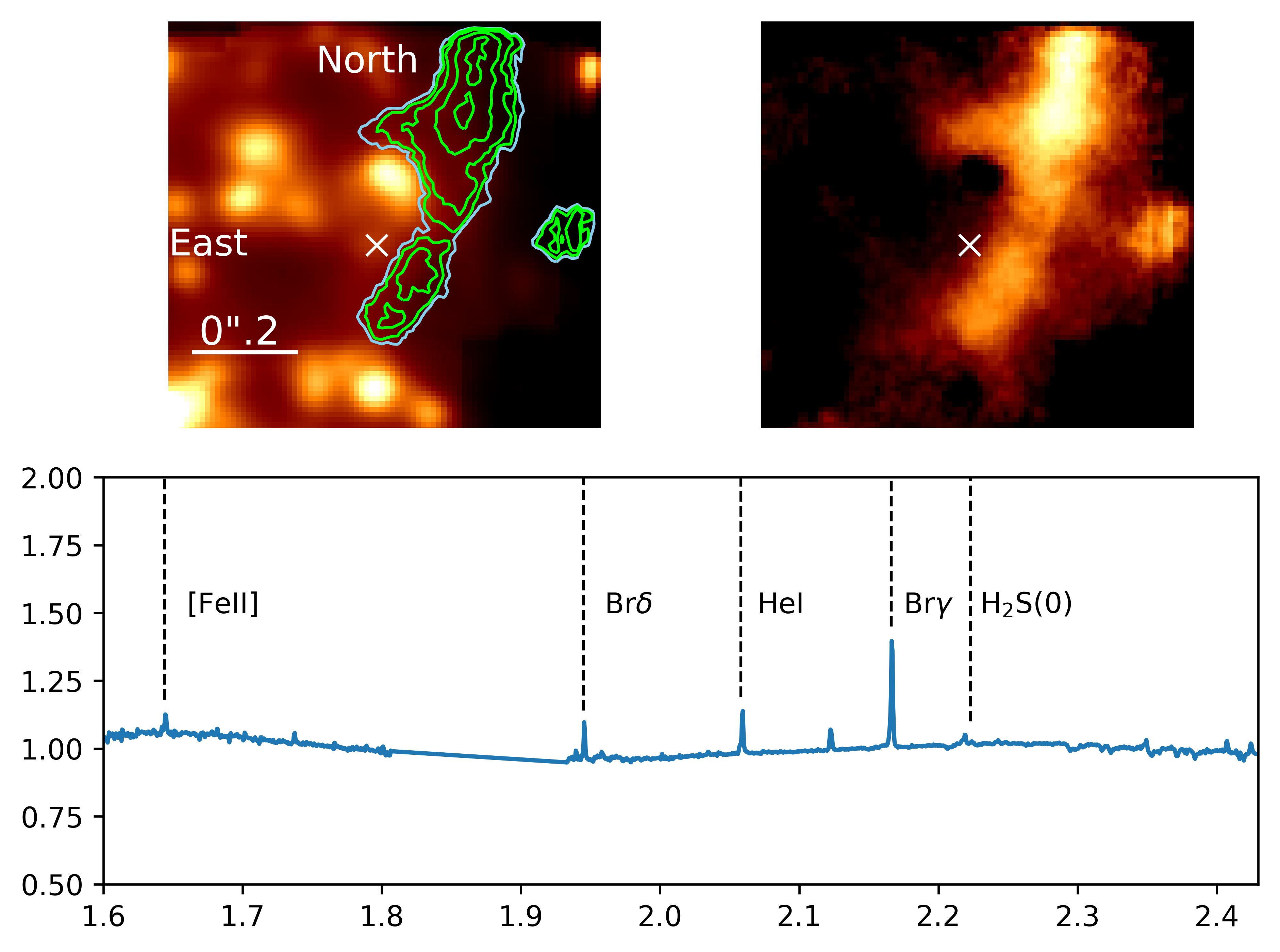
Figure 1: Combined SINFONI data-cubes between 2005 and 2015. The cubes are centered on the position of Sgr A* (marked with a white x). The upper left image shows the K-band continuum counterpart of the related data-cube. The green contours refer to the Br$\gamma$ line map emission shown in the upper right image. We set the levels of the green contours to 52.5$\%$, 56.5$\%$, 65$\%$, and 75$\%$. The light-blue contour line in the upper left image is set to 50$\%$.

The lower panel shows the spectrum for the Br$\gamma$-bar presented in the upper right image. The dashed line marks the rest-wavelength of the related emission. Another feature similar to the Br$\gamma$-bar can be seen at the right edge of the FOV (see upper left image and Sec. 3.3). The telluric emission between $1.80\,-\,1.93\mu m$ is flattened. The subtracted continuum emission of S2 in the upper right image results in a (an artificial) footprint in the investigated Br$\gamma$-bar. We note, that the croissant shape of S2 just above Sgr A* is an outcome of the co-adding.

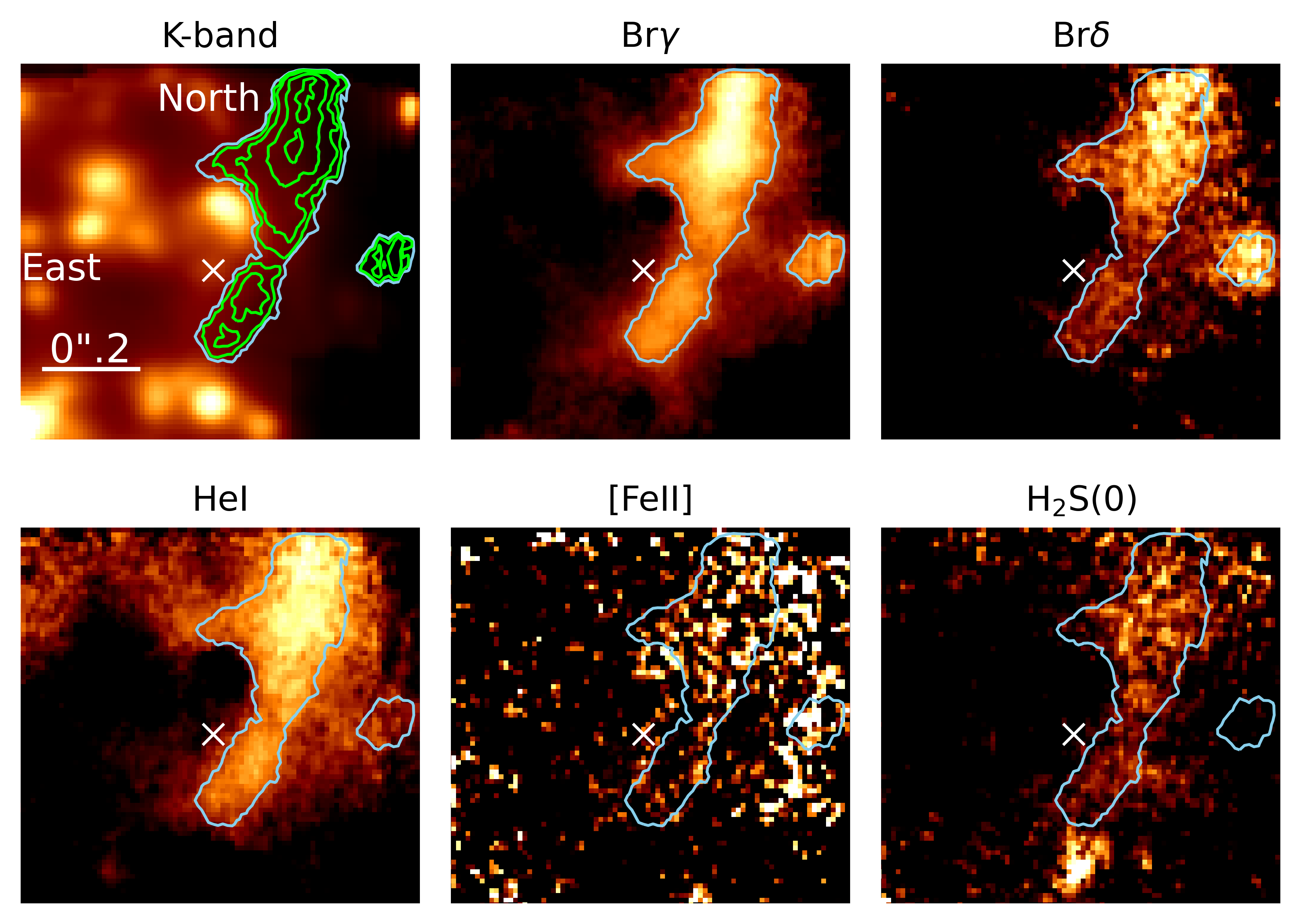
Figure 6: Line maps of the Br$\gamma$-bar L0. The upper left panel shows a K-band image of the GC based on the co-added data (see Fig. 1). For comparison, we add a 50% contour line (sky-blue) to the channel maps.

Since not every line reveals a strong counterpart image in its emission in the corresponding channel maps, we emphasize the investigation of the Br$\gamma$, Br$\delta$, HeI, [FeII], and H₂S(0) emission (see Table 1). These lines show clearly identifiable flux distributions and can be safely related to ionized emission of a gaseous bar (see Fig. 6). An outliers seems to be the blue-shifted H₂S(0) emission line. Even though we detect an extended related H₂S(0) line emission that can be clearly connected to the Br$\gamma$-bar, the Doppler-shift of this distribution indicates the presence and contribution of embedded and/or background/foreground objects (see the discussion in Sec. 4.6). For the sake of completeness, the line is still listed in Table 1.

Spectral line ($@$rest wavelength [$\mu$m])	central wavelength [$\mu$m]	Velocity [km/s]
[FeII] $@$1.64400 $\mu$m	1.64476 $\pm$ 0.00022	138.68 $\pm$ 40.14
Br$\delta$ $@$1.94509 $\mu$m	1.94548 $\pm$ 0.00010	60.15 $\pm$ 15.42
HeI $@$2.05869 $\mu$m	2.05951 $\pm$ 0.00017	119.49 $\pm$ 24.77
Br$\gamma$ $@$2.16612 $\mu$m	2.16650 $\pm$ 0.00010	52.62 $\pm$ 15.42
H2S(0) $@$2.22329 $\mu$m	2.21923 $\pm$ 0.00030	-547.83 $\pm$ 40.48

Table 1: Emission lines of the Br$\gamma$-bar based on the combined SINFONI data-cube combining data from observing periods obtained within a period of almost 10 years. The related spectrum is shown in Fig. 1.

We find, that the hydrogen recombination lines lie at a velocity of about 50-60 km/s and the lines that stand for a higher excitation ([FeII] and HeI) are at a higher velocity of a about 120-140 km/s. This may indicate that the hydrogen lines trace the bulk of our bar feature where as the higher excitation lines may be linked to a wind phenomenon (acting at its surface) resulting in a slightly higher redshift.

For the HeI/Br$\gamma$ ratio we find a value of 0.7 which is in agreement with the ratios of (0.35 - 0.7) observed in the GC (Gillessen et al., 2012). Compared to the surrounding Br$\gamma$ emission extended on larger scales, the intensity of the line at the position of the bar and especially of the clump-like enhancements therein varies by around $10\%$. We derive therefore a HeI/Br$\gamma$ ratio of $0.7\,\pm\,0.1$.

The extended Br$\gamma$ line emission as well as the MIR PAH1 continuum image (see Sec. 3.5) of the central few arcseconds clearly show a North-South as well as an East-West feature. Both contain substructures which are discussed in the following sections.

3.2 Substructures of the North-South Br$\gamma$-bar

In Fig. 1, we show a K-band image and a Br$\gamma$ channel map that is extracted from the combined data-cube that covers data sets obtained over a period of almost 10 years. The expected smearing effect due to proper motions of the features is significantly smaller than their extent and is eliminated by centering the individual data-cubes on the position of Sgr A*. Around 400 data-cubes with a single exposure time between 400-600s are used. With the clear detection of clumps (in the following indexed by $cl$) in the extended Br$\gamma$-features, we can determine the filling factor $f$ of these components as derived by

$$f\,=\,f_{\infty}\,+\,(1.0-f_{\infty})\exp\Big{(}-\frac{v}{v_{\rm cl}}\Big{)}\,\,\,\,.$$ (1)

This equation is introduced by Hillier et al. (2003). The authors use it to derive the filling factor for clumps that are created in the winds of two O-stars with a shared age of around 4.4 Myr in the Small Magellanic Cloud (SMC). Strong winds also prevail in the central region of the GC stellar cluster which justifies in combination with the recent publication by Calderón et al. (2020b) the use of Eq. 1. An effective use of the filling factor is described by Yusef-Zadeh et al. (2013) where the authors derive the number of clumps via $n_{cl}\,=\,f/(4/3\pi r^{3})$. For $f=1$ there would be no clumping. It is obvious, that a filling factor $f_{\infty}$ for the Br$\gamma$-bar far away from the observed emission is not equal to 1, but rather at lower values. Therefore, we assume an upper limit for $f_{\infty\,up}=$0.9 and a lower limit of $f_{\infty\,low}=$0.1 for equation Eq. 1. For $n_{cl}\,=\,2-4$ we derive values for $f$ close to 0.5.

The derived velocity $v_{cl}$ of the clumps in the Br$\gamma$-bar are based on the line-of-sight (LOS) velocity presented in Table 1. Mužić et al. (2010) state that the wind velocity $v$, prevailing in the S-cluster region, is about 750 km/s which is consistent with wind values derived by Najarro et al. (1994). With that, we derive an average filling factor of $f_{avg}\,=\,0.5$. From Gillessen et al. (2012), we use for the case B recombination of Br$\gamma$

$$\rho_{{\rm cl}} =2.6\times 10^{5}\left(\frac{f}{0.5}\right)^{-\frac{1}{2}}\left(\frac{R}{3\,{\rm mpc}}\right)^{-\frac{3}{2}}\times$$

$$\times\left(\frac{T}{10^{4}\,{\rm K}}\right)^{0.54}{\rm cm^{-3}}$$ (2)

where $\rho_{cl}$ donates the clump density. Following the analysis of Gillessen et al. (2012), we adapt the assumed electron temperature of $10^{4}$K (see also Zhao et al., 2009). With a radius of 75 mas/clump ($\hat{=}$ 3 mpc/clump) in the Br$\gamma$-bar, we get a mass per clump of

$$M_{\rm cl} =1.7\times 10^{28}\left(\frac{f}{0.5}\right)^{-\frac{1}{2}}\left(\frac{R}{3\,{\rm mpc}}\right)^{-\frac{3}{2}}\times$$

$$\times\left(\frac{T}{10^{4}\,{\rm K}}\right)^{0.54}{\rm g\,/cl}\,\approx\,2.1\,M_{\oplus}\,/{\rm cl}\,\,\,\,.$$ (3)

Since we detect around 4 individual clumps with comparable properties in the SINFONI FOV, we derive a lower limit for the mass of the observed Br$\gamma$-bar clumps of $8.4\,M_{\oplus}$ or $2.5\,\times\,10^{-5}\,M_{\odot}$. From the HeI/Br$\gamma$ ratio $\eta$, we get $\eta\,\approx\,0.7$. The Br$\gamma$ emission feature is obviously not homogeneous as can be seen in Fig. 1. In order for the presumably thin material to reproduce the line ratio $\eta$, the former derived volume filling factor of $\leq\,0.5$ is justified.

3.3 Substructures of the East-West Br$\gamma$-bar and additional gas reservoirs

Only the SINFONI data set of 2005 covers the area west of Sgr A*. Because of the limited data quality, we smooth the Br$\gamma$ line map with a 6 px Gaussian. Besides the Br$\gamma$-bar, we find several other gas reservoirs west of Sgr A* in different shapes. We name the detected features L0-L4 (see Fig. 2). Since these gas reservoirs are also seen in our VISIR continuum data (see Sec. 3.5), we are confident that the Br$\gamma$ gas emission areas are not remnants of the continuum subtraction. Peißker et al. (2020b) show several dusty sources with a presumably stellar core at the position of the Br$\gamma$ features L0 and L1. Both features show an angular difference of $\Delta\,=\,60^{\circ}$. Compared to the 226 GHz radio map presented by Yusef-Zadeh et al. (2017a) we find related counterparts to both L0 and L1. We speculate that also the additional gas and dust reservoirs associated with L2 - L4 (see Fig. 2) will contain compact dusty sources or young stellar objects.

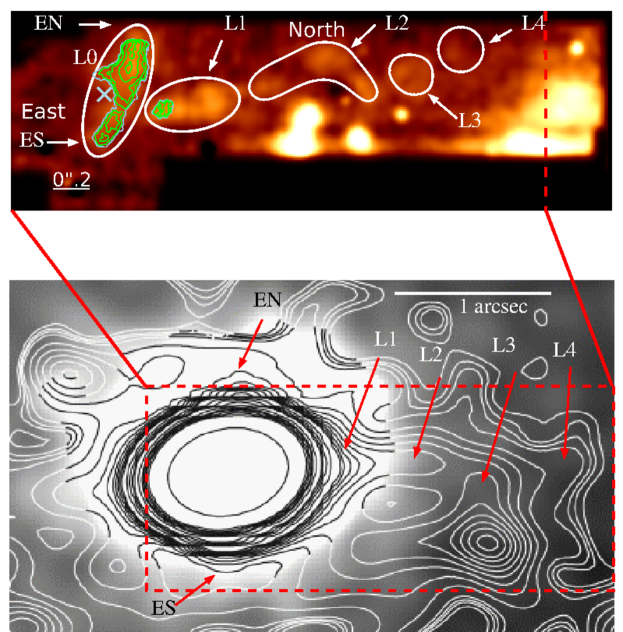
Figure 2: Galactic center in 2005. The upper panel shows a Br$\gamma$ line map of the SINFONI data cube smoothed with a Gaussian of 6 px. West of the north-south Br$\gamma$-bar (L0, the upper edge of the bar is marked with EN, the lower edgde with ES) we observe several gas reservoirs which are marked with arrows and white color. The estimated position of Sgr A* is indicated by a light-blue cross. The contour lines are adapted from Fig. 1. In the lower panel we show the same FOV in the 226 GHz radio domain as presented by Yusef-Zadeh et al. (2017a). We identify individual radio structures with source components detected at the positions of the Br$\gamma$ line flux in the infrared (see the upper panel)

.

3.4 Proper motion

By comparing the line maps of the Br$\gamma$-bar, that are centered on Sgr A*, a proper motion can be derived (Appendix, Fig. 5). As indicated by the contour maps shown in Fig. 1, we emphasize the analysis of the more prominent upper part of the Br$\gamma$-bar. To obtain the proper motion of this prominent part we use a cross-correlation method and additionally two Gaussian fitting methods (Fig. 3).

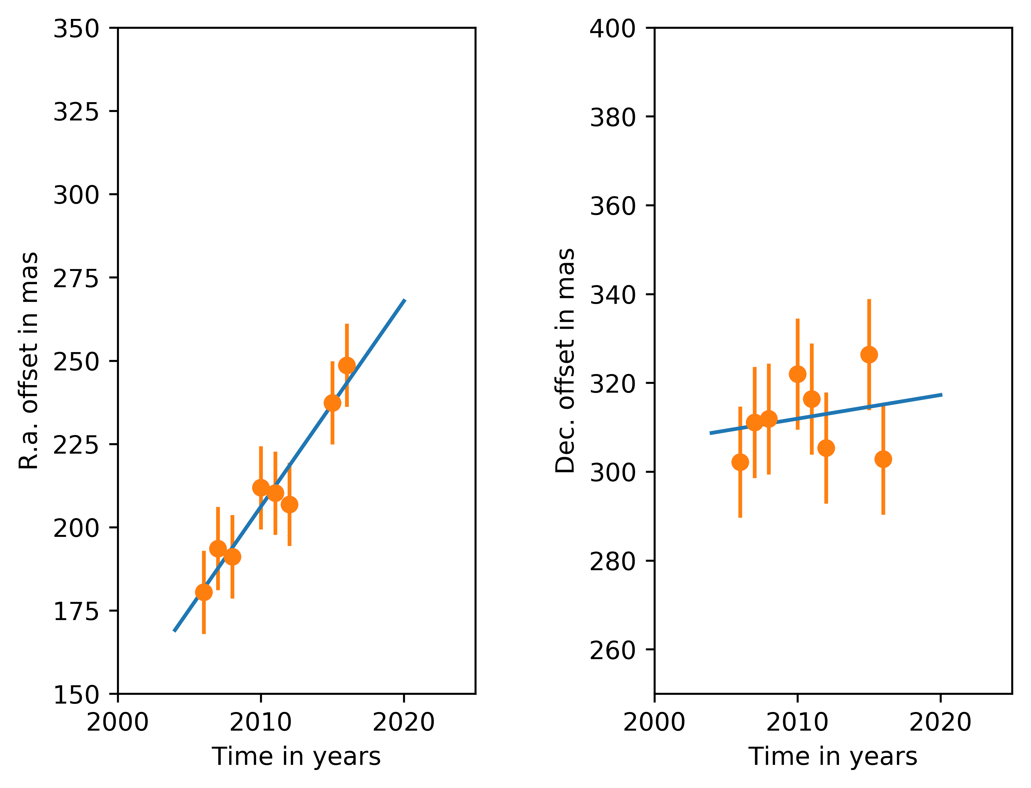
Figure 3: Proper motion of the prominent upper part of the Br$\gamma$-bar. The increasing distance of the bar towards Sgr A* indicates a linear proper motion. The declination-offset is close to constant and justifies the limitation on the x-shifting vector for the cross-correlation method. From the fit, we are deriving a proper motion of $319\,\pm\,44$km/s.

For the former method, we shift the Br$\gamma$ line map of 2018 to the 2006 position of the Br$\gamma$-bar and record, at which shifting vector the emission reaches its maximum. The shifting vector is then equivalent to the distance, that the feature moved projected on the sky. We find a proper motion of $329\,\pm\,20$km/s directed westward.
Since the Br$\gamma$ line flux distribution shows substructures (4 clumps, see Fig. 1), fitting a Gaussian to different substructures gives a complementary estimate of the velocities.

Year	R.A.	DEC.	$\Delta$R.A.	$\Delta$DEC.
	in [mas]	in [mas]	in [mas]	in [mas]
2006	180.50	302.16	-	-
2007	193.62	311.12	13.12	8.96
2008	191.16	311.88	10.66	9.72
2010	211.87	322.00	31.37	19.84
2011	210.25	316.37	29.75	14.21
2012	206.87	305.37	26.37	3.21
2015	237.37	326.37	56.87	24.21
2016	248.62	302.87	68.12	0.71

Table 2: Distance of the Br$\gamma$-bar. We measured the distance by using the substructures of the prominent upper part of the bar. The traveled distance $\Delta$R.A. and $\Delta$DEC. is related to the distance to 2006. The uncertainty is $\pm\,12.5$ mas and equivalent to $\pm\,1$ px.

Method	vR.A.	vDEC.	vtotal
	[km/s]	[km/s]	[km/s]
Cross-correlation (upper part)	117	307	329
Gaussian (upper part)	163	244	293
Gaussian (lower part)	153	252	295
Substructures (upper part)	209	241	319
Substructures (lower part)	114	293	314

Table 3: Proper motion in R.A. and DEC. with different methods. For fitting a Gaussian to the upper and lower part, we use pixel values between 10-12. The clumpy substructures can be fitted with an 5-6 px Gaussian. Note that we shift the data-cubes of 2006 and 2018 for the cross-correlation only in R.A. direction. Typical uncertainties for $v_{total}$ are in the order of $\pm\,40$ km/s, for $v_{R.A.}$/$v_{DEC.}$ around $\pm\,20$ km/s.

From this, we get velocities for R.A. and DEC. that are based on the fit parameters (Fig. 3). The resulting proper motion is $319\,\pm\,44$km/s directed westward. For the sake of completeness, we are fitting a Gaussian to the prominent upper part in 2006 and 2018. We crop the lower part of the data-cube to exclude extra emission. This results in a proper motion of $293\,\pm\,60$km/s. The error includes different background scenarios, a variation of data quality, and emission, that might be suppressed due to stellar emission lines.

Combining all three velocities, we get $314\,\pm\,41$km/s for the prominent upper part of the Br$\gamma$-bar. Using a Gaussian fit to substructures and the complete lower part, we derive a total proper motion of $305\,\pm\,15$km/s. In contrast, the proper motion vector of the lower part of the Br$\gamma$-bar points to South whilst the upper part is directed towards West. Consult Table 2 for the individual R.A. and DEC. proper motion velocities.

3.5 Mid-infrared detection

Based on the 2016 VISIR data set, we find at the position of the Br$\gamma$-bar in the N-band a PAH1 ($8.59\,\mu m$) counterpart with a width of $0.4\,\mu m$. The substructures shown in the contour plot in Fig. 1 are indicated in the low-pass filtered cutout in Fig.4, right hand side.

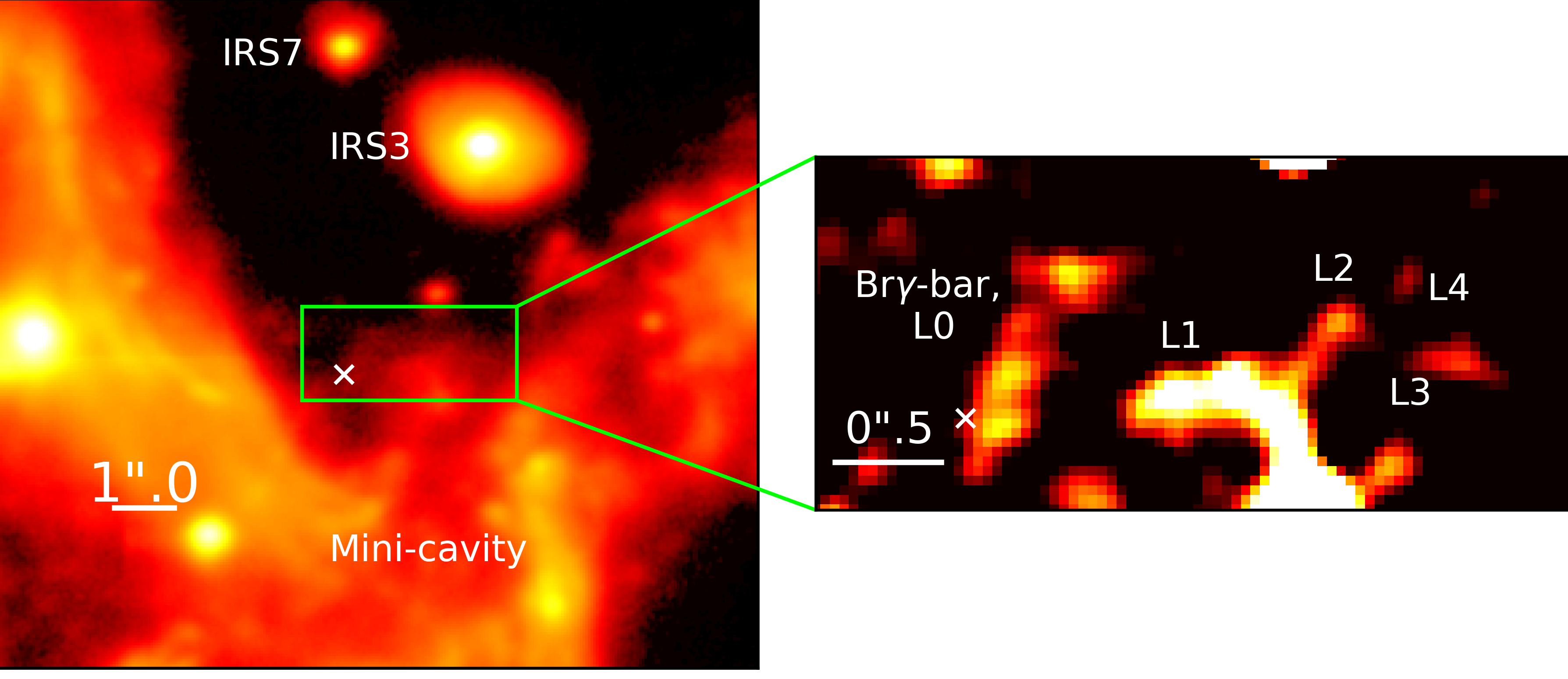
Figure 4: Overview of the GC in the MIR in 2016. The left image shows some prominent sources. The white cross marks the position of Sgr A*. The right image is a low-pass filtered cutout of the green box displayed in the left overview map. For the name IDs, please see Fig. 2. The position of Sgr A* was determined using the known positions of several SiO masers in the central cluster.

The size of the Br$\gamma$ line flux distribution is in good agreement with the PAH1 detection. The angular difference between the L1 to L0 component is $\Delta\,=\,60^{\circ}$ and consistent with the Br$\gamma$-bar orientation (Fig. 2). Since the FOV of SINFONI is limited, we find a small size difference of around $10-15\,\%$ compared to the VISIR detection which is already included in the uncertainties of the analysis presented here. Whilst the size of the Br$\gamma$-bar in our SINFONI data can be determined to be around 0”.95, the PAH1 continuum counterpart observed with VISIR extends over 1”.11.

3.6 226 GHz radio detection

The Br$\gamma$ features close to the line of sight towards Sgr A* can also be identified in the radio. Here, we refer to the radio maps published by Yusef-Zadeh et al. (2017b) and in particular to their Fig.2 where the authors show several linear ridge components. Unfortunately, the Br$\gamma$ features are very close to the Sgr A* position such that the corresponding identification can only be made via elongations on the lowest contours of the Sgr A* point source response.

Name ID	$\Delta$$\alpha$	$\Delta$$\delta$	description	S${}_{226\,GHz}$	SBrγ - expected	SBrγ - observed	extinction coefficient
	in [as]	in [as]	source size in [as]	in [mJy]	in [$10^{-17}\,Wm^{-2}$]	in [$10^{-17}\,Wm^{-2}$]	in [mag]
L0(EN/ES)	0.0 to -1.50	-0.3 to 0.4	ridge	$\sim$0.9	$\sim$1.27	1.11$\,\pm\,0.3$	$\sim$2.84
			$>0.8\,\times\,<0.2$
L1	-0.3 to -0.70	-0.14 to 0.06	ridge	1.3$\,\pm\,$0.4	1.84$\,\pm\,$0.6	1.54$\,\pm\,$0.6	2.97$\,\pm\,$0.7
			0.4$\times<0.2$
L2	-0.8 to -1.40	0.04 to 0.25	3 sources	1.3$\,\pm\,$0.4	1.84$\,\pm\,$0.6	1.55$\,\pm\,$0.4∗	2.94$\,\pm\,$0.6∗
			all $<0.2$
L3	-1.5 to -1.70	0.00 to 0.20	$<0.2$	1.2$\,\pm\,$0.3	1.70$\,\pm\,$0.4	1.31$\,\pm\,$0.4	3.26$\,\pm\,$0.8
L4	-1.8 to -2.00	0.10 to 0.30	$<0.2$	0.6$\,\pm\,$0.2	0.85$\,\pm\,$0.3	0.83$\,\pm\,$0.4	2.54$\,\pm\,$0.7

Table 4: Linear ridge components as outlined in Fig. 2. We list relative positions to Sgr A* and extent of the aperture within which most of the flux is contained, description of the source component and a limit on the size, 226 GHz flux densities based on the observations by Yusef-Zadeh et al. (2017a) and expected Br$\gamma$ line fluxes calculated with Eq. 4. The observed flux is based on the SINFONI H+K data cubes. The last column shows the derived extinction coefficient. The identification of the sources west of Sgr A* is guided by the shape of the radio contours. Size estimates and distances are given in arcseconds. Note: the (^∗) marks 3 single detections that are, based on the radio observation, grouped together as L2. The errors of the expected Br$\gamma$ flux is pervaded from the observed radio detection. The radio flux for the L0 component is not known. Here, it is assumed to be on the same order as the flux densities of the other components. The uncertainties of the observed Br$\gamma$ flux is based on the SINFONI flux analysis.

In Fig. 2 we compare the smoothed Br$\gamma$ map with the radio map. In Table 4 we list the components names, the relative coordinates and their 226 GHz fluxes. We identify the northern and southern radio extensions marked EN and ES with the northern and southern tip of the north-south (NS) Br$\gamma$ feature. The western Br$\gamma$ feature can be identified as the extension labeled $L1$. It is followed by the curved source complex labeled $L2$ and the extended (0.15 to 0.2 arcseconds diameter) sources $L3$ and $L4$. The 226 GHz radio flux density of these components can be estimated from their extent and the contour line labels given in Fig.2 by Yusef-Zadeh et al. (2017b).

The east-west linear feature L1 appears to arise from Sgr A*. Yusef-Zadeh et al. (2017b) points out that it coincides with the diffuse X-ray emission and a minimum in the near-IR extinction. They argue that the millimeter emission is produced by synchrotron emission from relativistic electrons in equipartition with an $\sim$1.5 mG magnetic field.

Yusef-Zadeh et al. (2017b) argue that the linear ridge may become brighter close to the peak of Sgr A* at 226 GHz and may therefore have a hard or highly inverted spectrum since there is no detectable emission of it at lower frequencies. However, at lower frequencies the beams typically become larger and sources close to Sgr A* are more difficult to be detected. Hence, the scenario could also be compatible with a flat spectrum Bremsstrahlung source.

Yusef-Zadeh et al. (2017b) point out that in the recent milli-arcsec resolution, the 86 GHz and 230 GHz observations of Sgr A* show indications of an asymmetric source structure (Brinkerink et al., 2016; Fish et al., 2016). Towards the east under a position angle of about 90 degrees, a secondary source shifted by 100 micro-arcsec from Sgr A* is indicated by the data. While this could be explained by interstellar scattering (Brinkerink et al., 2016), intrinsic source properties could be responsible as well.

However, given the proper motion of the ridge component L0 in the order of 320 km/s, it is very likely that it is part of the minispiral gas flow. Since L1 is comparable in shape and size to L0, it is very likely that the east-west feature could also be part of this gas flow.

Assuming an optically thin free-free emission spectral index of 0.1 between 5 GHz and 226 GHz and an intrinsic Br$\gamma$/Br$\alpha$ ratio of 2.8, we can estimate the expected Br$\gamma$ line intensity from the 226 GHz radio continuum flux density using the formula (Glass, 1999)

$$\begin{split}&I({\rm Br}\gamma)=\\ &1.42\times 10^{-17}\left(\frac{T}{10^{4}\,{\rm K}}\right)^{-0.85}\left(\frac{\nu}{226\,{\rm GHz}}\right)^{0.1}F_{\nu}({\rm mJy})~{}{\rm Wm^{-2}}\end{split}$$ (4)

We then compare the predicted flux density $I(Br\gamma)$ to the observed flux density that is based on the SINFONI Br$\gamma$ line map detection. These maps are related to the channels 1515-1520 that corresponds to $2.16527\,\mu m$ and $2.16825\,\mu m$. From the ratio of the expected to observed flux density, we obtained an estimate of the extinction in the mini-spiral region at $2.16\,\mu m$. The results are listed in Table 2.

The observed extinction ranges from 2.5-3.2 mag, with an averaged extinction of $2.91\,\pm\,0.72$ mag (see Table 4). This is in good agreement with Schödel et al. (2010), who reported a median extinction value of $A_{K_{s}}=2.74\,\pm\,0.30$ mag in the range of 1.8-3.8 mag in the mini-spiral arms, using H-K colors.

4 Discussion

In this section we will discuss the results of our analysis. We also link the observed filaments to large scale features in the region.

4.1 Distance estimate of Br$\gamma$ bar and its stability in the hot bubble

Based on the tangential velocity of $v_{\rm t}\sim 314\,{\rm km\,s^{-1}}$ and the radial velocity of the bar $v_{\rm r}\sim 53\,{\rm km\,s^{-1}}$ (based on the Br$\gamma$ emission line), we estimate the total space velocity using $v_{\rm bar}\sim(v_{\rm t}^{2}+v_{\rm r}^{2})^{1/2}\sim 318\,{\rm km\,s^{-1}}$. From this, we may approximately calculate the distance from Sgr A* assuming a bound circular orbit, $r_{\rm bar}\sim GM_{\bullet}/v_{\rm bar}^{2}\sim 0.17\,(M_{\bullet}/4\times 10^{6}\,M_{\odot})(v_{\rm bar}/318\,{\rm km\,s^{-1}})^{-2}\,{\rm pc}\sim 4.25^{\prime\prime}$. In case the Br$\gamma$ is unbound and moving along the parabolic orbit, the distance would be a factor of two larger, $r_{\rm bar}^{\rm esc}\approx 2GM_{\bullet}/v_{\rm bar}^{2}\sim 0.34\,{\rm pc}=8.5^{\prime\prime}$. In the following discussion, we assume the bar is bound and hence the smaller distance estimate applies.

The associated orbital (dynamical) timescale is $t_{\rm dyn}\sim 2\pi[r^{3}/(GM_{\bullet})]^{1/2}\sim 3300$ years. This applies for the more prominent westward-moving upper part of the Br$\gamma$ bar. Additionally, we derive similar values for the southward-moving lower part of the bar, specifically we determine $r_{\rm bar}\sim 0.18\,{\rm pc}$ and $t_{\rm dyn}\sim 3600$ years.

With $r_{\rm bar}\sim 0.17\,{\rm pc}$, the Br$\gamma$ bar is located at or just beyond the Bondi radius, $r_{\rm Bondi}\sim GM_{\bullet}/c_{\rm s}^{2}$, where $c_{\rm s}$ is the sound speed of the hot gas that is fueled mostly by OB stars. This hot plasma has the temperature of $T_{\rm Bondi}\sim 10^{7}\,{\rm K}$ and the number density of $n_{\rm Bondi}\sim 26\,{\rm cm^{-3}}$, from which $r_{\rm Bondi}\sim 4^{\prime\prime}(T_{\rm Bondi}/10^{7}\,{\rm K})\sim 0.16\,{\rm pc}$ (Baganoff et al., 2003; Wang et al., 2013). In terms of stellar populations, the Br$\gamma$ bar can be found at larger scales than the S-cluster ($1^{\prime\prime}\sim 0.04\,{\rm pc}$), potentially within the Clockwise Disk (CWD) of young massive OB stars located between $0.032-0.48\,{\rm pc}$ (Bartko et al., 2009). The derived distance is also comparable to the pericentre distances of the Northern and the Eastern Arm streamers of the minispiral (Zhao et al., 2009), $q_{\rm NA}\simeq 0.17\,{\rm pc}$ and $q_{\rm EA}\simeq 0.25\,{\rm pc}$, respectively, which raises the possibility that the Br$\gamma$ bar is a detached minispiral material that appears to be positioned close to Sgr A* just in projection. The Br$\gamma$ bar could also have originated in the collision site of the Northern and the Eastern arm, so-called the Bar, located at $\sim 0.1-0.2\,{\rm pc}$ south of and behind Sgr A* (Zhao et al., 2010).

When one compares the gas pressure of the bar, $P_{\rm bar}=n_{\rm bar}k_{\rm B}T_{\rm bar}\sim 2.6\times 10^{5}\,{\rm cm^{-3}}\times 1.38\times 10^{-16}\,{\rm erg\,K^{-1}}\times 10^{4}K\sim 3.588\times 10^{-7}\,{\rm erg\,cm^{-3}}$, with the pressure of the bremsstrahlung plasma at the Bondi radius, $P_{\rm Bondi}=n_{\rm Bondi}k_{\rm B}T_{\rm Bondi}=26\,{\rm cm^{-3}}\times 1.38\times 10^{-16}\,{\rm erg\,K^{-1}}\times 10^{7}\,{\rm K}\sim 3.588\times 10^{-8}\,{\rm erg\,cm^{-3}}$, we see that the bar pressure is larger than the pressure at the Bondi radius by one order of magnitude. This implies that the bar is not confined by the surrounding thermal pressure. In that case, the bar expands with a velocity approximately equal to its sound velocity, $v_{\rm exp}\sim c_{\rm bar}=[k_{\rm B}T_{\rm bar}/(\mu m_{\rm H})]^{1/2}\sim 13\,{\rm km\,s^{-1}}$.
Due to the relative motion of the bar and the ambient medium fueled by stellar winds, the force arises on the bar because of to the ram pressure, $P_{\rm ram}\sim\rho_{\rm Bondi}v_{\rm rel}^{2}$, where the relative velocity is the vector sum of the bar motion with respect to the stellar wind velocity field. Given $v_{\rm bar}\sim 318\,{\rm km\,s^{-1}}$ and the average stellar-wind velocity of $v_{\rm wind}=750\,{\rm km\,s^{-1}}$ (Najarro et al., 1994), we set $v_{\rm rel}\sim 10^{3}\,{\rm km\,s^{-1}}$. The ram pressure then is $P_{\rm ram}=\mu m_{\rm H}n_{\rm Bondi}v_{\rm rel}^{2}=0.5\times 1.67\times 10^{24}\,{\rm g}\times 26\,{\rm cm^{-3}}\times(10^{8}\,{\rm cm\,s^{-1}})^{2}\sim 2.2\times 10^{-7}\,{\rm erg\,s^{-1}}$. The ram pressure is of a comparable order of magnitude as the thermal pressure of the Br$\gamma$ bar, and hence can confine the bar externally or at least influence its further evolution.

Moreover, dynamically important magnetic field in the vicinity of Sgr A* can affect the evolution of Br$\gamma$ bar more than the combined effect of the ram pressure and the external thermal pressure. The magnetic pressure can be estimated from the Faraday rotation measurements of the magnetar PSR J1745-2900, which is located at the comparable distance as the Br$\gamma$-bar, $r\gtrsim 0.12\,{\rm pc}$ from Sgr A*. The Faraday rotation measurements indicate a line-of-sight component of the magnetic field of $B\gtrsim 8\,{\rm mG}$ (Eatough et al., 2013), from which the magnetic pressure can be estimated as $P_{\rm mag}=B^{2}/8\pi\approx 2.6\times 10^{-6}\,{\rm erg\,cm^{-3}}$ and we see that $P_{\rm mag}>P_{\rm bar}$. It is now premature to say whether the Br$\gamma$-bar belongs to the filamentary structures such as nonthermal filaments that follow the global magnetic field lines. Morris et al. (2017a) reported about the thin filamentary structure to the north and the east of Sgr A*, so-called Sgr A West Filament (SgrAWF). In their radio images at centimeter wavelengths as well as Pa$\alpha$ image, one can also see the potential counterparts of the L0-L4 complex to the west of Sgr A*. We hypothesize at the moment that the Br$\gamma$ bar reported here could be the manisfestation of the minispiral material which is shaped and dynamically affected by the global poloidal magnetic field in a similar way as SgrAWF or by the external magnetohydrodynamic drag. However, more multiwavelength data is necessary to make definite conclusions. We discuss more mechanisms responsible for clumpy filamentary structures in the Galactic center region in the following subsections.

The bar as a whole will inevitably tend to be tidally stretched since its number density expressed by Eq. 2 is five orders of magnitude smaller than the Roche condition of the self-gravitational collapse derived for fully ionized plasma at the estimated distance of the bar,

$$\begin{split}&n_{\rm bar}\ll n_{\rm Roche}\,=\,\\ &4.73\times 10^{10}\left(\frac{M_{\bullet}}{4\times 10^{6}\,M_{\odot}}\right)\left(\frac{r}{0.17\,{\rm pc}}\right)^{-3}\,{\rm cm^{-3}}\,.\end{split}$$ (5)

In addition, the tidal radius $r_{\rm t}$ for the bar half-length of $R_{\rm bar}\sim 0.5^{\prime\prime}\sim 0.02\,{\rm pc}$ (based on SINFONI and VISIR), the estimated bar mass of $m_{\rm bar}\approx 2.5\times 10^{-5}\,M_{\odot}$, and the Sgr A* mass of $M_{\bullet}=4\times 10^{6}\,M_{\odot}$ is

$$r_{\rm t} =R_{\rm bar}\left(\frac{2M_{\bullet}}{m_{\rm bar}}\right)^{1/3}=$$

$$=137\left(\frac{R_{\rm bar}}{0.5^{\prime\prime}}\right)\left(\frac{m_{\rm bar}}{2.5\times 10^{-5}\,M_{\odot}}\right)^{-1/3}\,{\rm pc}\,,$$ (6)

hence the bar is prone to the complete tidal disruption since it moves around Sgr A* at $r\approx 0.2\,{\rm pc}$, which is three orders of magnitude closer than $r_{\rm t}$. One still cannot exclude the possibility that Br$\gamma$ bar is a filamentary, clumpy structure, which is being overall tidally disrupted, but individual clumps would be self-gravitating with number densities of the order of the Roche critical density, see Eq. (5). These clumps would, however, have to be very compact with length-scales of a few AU, which follows from the Hill radius,

$$r_{\rm Hill} =r_{\rm bar}\left(\frac{m_{\rm cl}}{3M_{\bullet}}\right)^{1/3}=$$

$$=3.13\left(\frac{r_{\rm bar}}{0.17\,{\rm pc}}\right)\left(\frac{m_{\rm cl}}{2.1\,M_{\oplus}}\right)^{1/3}\,{\rm AU}.$$ (7)

Individual clums could also hide stars that would be enshrouded in optically-thick gaseous-dusty shells with the length-scale of $r_{\rm Hill}\sim 153\,{\rm AU}$ (Zajaček et al., 2014; Valencia-S. et al., 2015; Shahzamanian et al., 2016; Zajaček et al., 2017), which follows directly from Eq. (7) for $m_{\rm cl}=1\,M_{\odot}$. However, any association of the Br$\gamma$ bar with the population of dust-enshrouded objects (Peißker et al., 2020b; Ciurlo et al., 2020) is currently speculative and requires additional monitoring of the dynamics of this Br$\gamma$ complex.

For estimating the lifetime and the stability of the Br$\gamma$ bar, we follow Burkert et al. (2012), who derived basic timescales for the interaction of a colder clump, in our case a filament or a streamer, with the surrounding hot medium. The ablation of material due to the motion through the hot medium is rather slow with the ablation timescale of

$$\tau_{\rm abl} =\frac{R_{\rm bar}}{0.25q_{\rm abl}v_{\rm bar}}\frac{\rho_{\rm bar}}{\rho_{\rm Bondi}}=6\times 10^{8}\left(\frac{R_{\rm bar}}{0.02\,{\rm pc}}\right)\times$$

$$\times\left(\frac{v_{\rm bar}}{318\,{\rm km\,s^{-1}}}\right)^{-1}\left(\frac{\rho_{\rm bar}/\rho_{\rm Bondi}}{10000}\right)\,{\rm yr}\,,$$ (8)

where we considered $q_{\rm abl}\approx 0.004$. The evaporation due to thermal conduction proceeds much faster. In the saturation limit and assuming pressure equilibrium (that may not apply as we estimated earlier), we obtain

$$\tau_{\rm evap}\approx 177\,\left(\frac{r_{\rm bar}}{0.17\,{\rm pc}}\right)^{1/6}\left(\frac{m_{\rm bar}}{2.5\times 10^{-5}\,M_{\odot}}\right)^{1/3}\,{\rm yr}\,,$$ (9)

which is an order of magnitude less than the dynamical timescale of a few thousand of years. This implies that the Br$\gamma$ bar is likely a temporary feature that will not survive long enough to affect the activity of Sgr A*, since the free-fall timescale from $r_{\rm bar}$ is,

$$t_{\rm ff}=\pi\left(\frac{r_{\rm bar}^{3}}{GM_{\bullet}}\right)^{1/2}\sim 1643\,{\rm yr}\,.$$ (10)

Due to the velocity shear between the bar and the Bondi plasma, the bar is susceptible to the Kelvin-Helmholtz (KH) instability. The velocity shear can be assumed to correspond to the orbital velocity of the bar, $v_{\rm shear}\sim v_{\rm bar}\sim 318\,{\rm km\,s^{-1}}$. Given the density ratio of $r=n_{\rm Bondi}/n_{\rm bar}\sim 10^{-4}$ between the hot plasma and the bar, the instabilities of the size comparable to individual clumps, $\lambda_{\rm cl}\sim 3\,{\rm mpc}$, will develop on the timescale of

$$\tau_{\rm KH}=\frac{\lambda_{\rm cl}}{v_{\rm shear}}\frac{1+r}{\sqrt{r}}\approx 923\,{\rm years}\,.$$ (11)

Hence, the KH instabilities with the size comparable to the observed clumps can develop within one orbital (free-fall) timescale and the observed uneven surface brightness of the Br$\gamma$ structure can already be a manifestation of this process. The magnetic field can in theory suppress the formation of Kelvin-Helmholtz instabilities and stabilize the structure, especially if the internal tangled magnetic field is present in the bar structure itself (McCourt et al., 2015). On the other hand, as found in McCourt et al. (2015), the structure would still fragment into clumps that would not mix into the hot medium but rather co-move with it. Hence, the bar would continue to change its appearance and the surface brightness during the timescales derived above.

In summary, the Br$\gamma$ bar is a temporary feature that will likely disappear within 100–1000 years due to the combined action of evaporation, tidal stretching, and instability development. Given its estimated distance of $r_{\rm bar}\sim 0.2\,{\rm pc}$ from Sgr A*, it is unlikely to affect its activity since the free-fall timescale is longer than both the evaporation and the instability timescale. These conclusions could in principle be affected by a complicated interplay of different components in the central parsec (minispiral, stars, Sgr A*, dust). For instance, if the bar was formed due to the stellar wind-wind collisions as modelled by Calderón et al. (2016, 2020b), the structure can be continuously recreated and/or formed elsewhere depending on the spatial distribution of stars inside the nuclear star cluster. However, Calderón et al. (2020a) analyzed the cold clump formation via the non-linear thin shell instability in the wind-wind interaction and found a small mass of individial clumps in the range of $\sim 10^{-3}-10^{-2}\,M_{\oplus}$, which is much smaller than the mass of a few Earth masses inferred for the clumps along the bar. This makes the association of the Br$\gamma$ bar with the minispiral streamers more likely since the Northern and Eastern streamers alone contain $\sim 12\,M_{\odot}$ of ionized gas (Zhao et al., 2010). We will discuss the relation of the bar to other structures in the GC region in the following subsections.

4.2 Thin filaments of the GC

As shown by Mužić et al. (2007), elongated and narrow filaments in the vicinity of Sgr A* seem to be the rule and not the exception (see also Ciurlo et al., 2014, 2019).

Even on larger scales compared to the observations presented in Mužić et al. (2007), filaments with a specific orientation with respect to the central region associated with Sgr A* can be observed. Examples are presented, e.g. in the inner $1^{\circ}\times 1^{\circ}$ by LaRosa et al. (2004). Here, the authors characterize their detection as non-thermal filament (NTF) candidates (for larger scales see also Yusef-Zadeh et al. (2005); Morris et al. (2017b)). Since the Br$\gamma$ feature we investigate here, is presumably influenced by the UV radiation of hot massive young He-stars (Yusef-Zadeh et al., 1996; Carlsten & Hartigan, 2018; Kim et al., 2018) at the center of the GC stellar cluster potentially including the S-stars, the gas can very likely considered to be a thermal filament (TF) dominated by Bremsstrahlung emission (see Sec. 4.4). However, the NTF candidates morphology is shaped by the magnetic fields of the GC. These magnetic fields imply a non-poloidal shape which results furthermore in a complex structure. In order to differentiate between the TF and NTF character of the filaments, polarization measurements of the features at high angular resolutions are needed.

As shown in Sec. 3.4, the proper motion of the upper part of the Br$\gamma$-bar is around 320 km/s and therefore comparable with the proper motion of other filaments detected in the infrared in the vicinity of Sgr A*. For example, following the nomenclature by Mužić et al. (2007), NE3, NE4, and SW7 are showing proper motions that are in the same range.

4.3 Location of the Br$\gamma$ bar features

While the Br$\gamma$ bar features we describe here are located close to the line of sight towards Sgr A*, one can raise the question of what their true physical distance to the SMBH and the S-star cluster is. Very close proximity to Sgr A* on scales of the S-cluster members would imply high orbital velocities of several hundred to a few thousand km/s. Also the gaseous features would likely be distorted rather than almost linear. Hence, it is unlikely that they are in the immediate vicinity of Sgr A*. However, they could be part of the general mini-spiral flow. It seems peculiar that they are located in projection north of Sgr A* rather than south were the bulk of the material is passing by Sgr A*. However, ALMA observations show that in the central few arcsecond and just north of Sgr A* complex, extended emission can be found in the emission of density tracers like CS and H₃CO⁺ (Moser et al., 2017). In fact, kinematic modeling of the gaseous mini-spiral material indicates that the gas is rather turbulent.

Vollmer & Duschl (1999) present a self-consistent hydrodynamic model of the gas flow in the mini-spiral system. They model the mini-spiral gas streams as three disk systems that are interleaved and form structures like the northern arm and the mini-spiral bar feature. In their modeling, the authors relate to the observations of the Sgr A West complex in the H92$\alpha$ line at 8.3 GHz with a resolution of 1 arcsec as presented by Roberts & Goss (1993) as well as the [Ne II]($\lambda\,12.8\mu$m) line emission observations described in detail by (Lacy et al., 1991). Similar models of the mini-spiral gas have also been put forward by e.g. Zhao et al. (2009) or Tsuboi et al. (2017).

In order to match the observations, Vollmer & Duschl (1999) allow for an ad-hoc radial accretion velocity of 5% of the local Keplerian azimuthal velocity. They also find, that a satisfactory description of the data is only possible if they allow for a disk-like flow with a turbulent velocity of 40% of the Keplerian velocity, and a vertical turbulent velocity of 5% of the Keplerian velocity. The turbulent velocities determine the thickness and viscosity of the disk.

The authors point out that in the framework of the standard theory of accretion disks (see, e.g Frank et al., 1992), this corresponds to a viscosity parameter $\alpha\,\sim\,0.3$. This is a value which is well within the range found for other types of disks. In Fig.17 of Vollmer & Duschl (1999), the authors plot the modeled disk material at low intensity levels and find that a tenuous gas component may fill almost the entire planes that represent gaseous stream of the northern arm and the bar.

Therefore, it seems conceivable that the Br$\gamma$-bar features we report are part of the turbulent mini-spiral as a stream that passes by Sgr A* from behind (see geometry of the model presented by Vollmer & Duschl (1999)). This is consistent with the fact that no strong temporal variations in extinction, i.e. reddening, towards the S-cluster members or even the infrared counterpart of Sgr A* have been reported.

4.4 Stellar wind induced ionization

Based on the detection of the bar throughout the available SINFONI data, the emission of the ionized feature in the vicinity of Sgr A* is the focal point of several phenomena in the GC. The case B recombination lines imply UV radiation by the surrounding stars (Najarro et al., 1994, 1997; Martins et al., 2007). The authors of Karas et al. (2019) model the combination of a wind originating in a stellar cluster and the ISM and describe two shocks: a wind stellar wind shock and a jet-shock induced by the ISM. The transition zone between the wind- and jet-shock, that harbors clumps, is discussed in the following subsection. Calderón et al. (2016, 2020b) modeled and discussed the influence of the stellar winds of the Stars in the GC on scales of a few parsecs. Ressler et al. (2018) shows even closer simulations of the inner parsec. The massive and luminous He-stars are the major wind sources. The lower luminous S-cluster stars may contribute to the wind impact onto the filaments only in the case where the Br$\gamma$ filaments we describe here are close to the central arcsecond. The authors describe that the S-star S2 and complex structures in the accretion wind have an influence on the low accretion rate that they derive to be a few $\times\,10^{-8}\,M_{\odot}\,yr^{-1}$.

4.5 Shock induced clumpiness

As shown in Fig. 1, the spectrum of the Br$\gamma$-bar shows a prominent [FeII] and H₂ line. Both emissions are indicators for shocks induced by stellar winds of young OB stars or an accretion wind onto and from Sgr A*. As already mentioned in Sec. 3.1, the H₂S(0) line seems to be connected to a different object because of the large blue-shifted line-of-sight velocity (see discussion in Sec. 4.6).

However, the [FeII] emission can be associated with fast collisions of winds and gas clouds and as a consequence, shocks could be the reason for the ionization of the gas (Mouri et al., 2000). These shocks could then also be responsible for the observed and detected clumps as already simulated and discussed by Calderón et al. (2016). Our estimated lower mass limit of $2.5\,\times\,10^{-5}\,M_{\odot}$ is consistent with the mass, that the authors derive for the clumps that are created by the collision of stellar winds produced by the S-stars.

4.6 The blue-shifted H₂S(0) line

We find, that the L0 Br$\gamma$-bar feature is located at the position of the gap seen in the ALMA detection of a rotating disk structure (Murchikova et al., 2019). The authors report, that the gap separates the red- and blue-shifted part of the disk spectrum. Within the uncertainties and the width of the rotating ALMA disk spectrum, our Br$\gamma$-bar feature L0 may be responsible for an absorption resulting in the detected gap (see corresponding comment in Murchikova et al., 2019). This would make the bar feature a foreground object with respect to the structure detected with ALMA. Alternatively, the Br$\gamma$-bar L0 could be located at the center of the rotating ALMA disk, absorbing only the background disk emission. If the disk is orbiting Sgr A* this would position the bar feature close to the center. This, however, would imply a high velocity spread (several 100 km/s, similar to the S-star cluster members) of the gas constituting the bar feature. This is not observed, hence, making this explanation a more challenging and a though less likely one.

4.7 Upcoming MIRI observations

Considering the mid-infrared detection of features close to Sgr A*, the upcoming MIRI instrument on board of the James-Webb-Space-Telescope (JWST) (consider Bouchet et al., 2015; Rieke et al., 2015; Ressler et al., 2015) is a reasonable opportunity for observations. Even though the plate scale of MIRI is slightly increased compared to SINFONI, the size of the observed features ensure a continuum detection with MIRI. This is even more true considering the comparable plate scale of VISIR and NIRSpec and the detection of the Br$\gamma$-bar in the MIR (see Fig. 4). With NIRSpec we will have also access to a confusion free Doppler shifted Pa$\alpha$ emission line because of the not present telluric absorption and emission features. We are expecting a more complete picture of the observed structures. With the spectroscopic capabilities of MIRI, we will have broad band information about several emission lines like e.g., $CO$, $SiO$, and $CH_{4}$ (Peißker et al., 2020b). The stable point spread function of the JWST will also help to image faint and extended features in the central stellar cluster.

5 Conclusions

In this work, we have shown that the Br$\gamma$-bar located to the west of Sgr A* is in projection close to the S-cluster and exhibits a proper motion of around 320 km/s in westward direction. This velocity matches proper motion values of other infrared and radio features traced in that region (Yusef-Zadeh et al., 2004; Mužić et al., 2007; Yusef-Zadeh et al., 2017b). Altough it is close to Sgr A* in the line of sight, we argue that it is at least part of the mini-spiral passing by the very center. We find substructures that indicate a clumpiness that are most plausibly caused by the shocks of stellar winds. The lower limit for the mass of the observed Br$\gamma$-bar feature in the SINFONI FOV is $2.5\,\times\,10^{-5}\,M_{\odot}$. This value is in agreement with models about stellar wind interactions in the direct vicinity of Sgr A*. For this, we assumed a stellar wind velocity of 750 km/s. We find several indications, that the observed Br$\gamma$ feature is influenced by wind and shock interactions with the ISM west of Sgr A*. From the presented analysis, we suggest that the feature shows infrared line emission associated with a radio Bremsstrahlung filament. We can conclude, that we need more data that covers the area north and west of Sgr A* to investigate the full size of the feature in the NIR or additional gas reservoirs. Since we also observe another prominent Br$\gamma$-bar L1 west of Sgr A* (prominent in the MIR continuum emission), we are confident that observations with the JWST and future instruments like ERIS at the VLT will produce a more complete picture about the line emission features and filaments in the vicinity of Sgr A*. It is possible that the gas reservoir associated with the extended feature can be connected to the dusty objects also present in this region. They could be indicators of ongoing star formation in the central region of the stellar cluster harboring Sgr A*. Long term observations will complete this speculative connection.

Appendix A Proper motion measurements and individual blobs

As described in Sec. 3.4, we use different methods in order to derive a proper motion based on the prominent upper part.

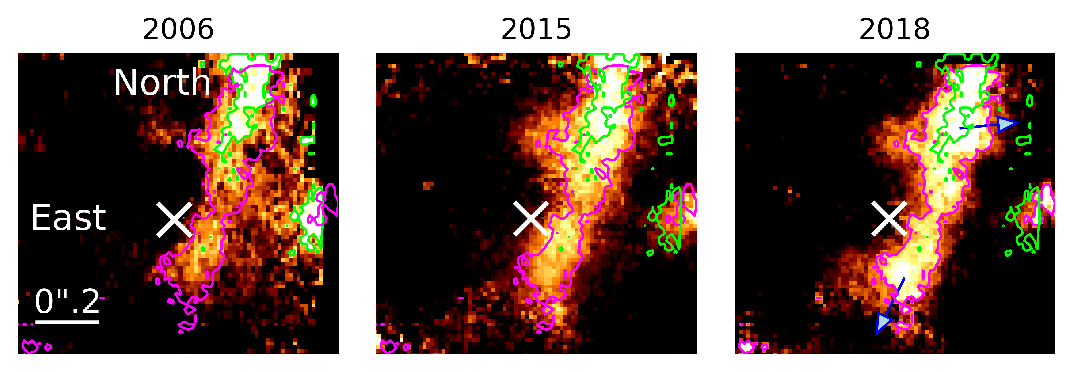
Figure 5: The central few arcseconds of the Galactic center in 2006, 2015, and 2018. The proper motion vector for the prominent upper part is pointing towards the west with a proper motion of around 320km/s. The southern part of the bar is moving towards the south-east with a proper motion velocity of about 314km/s. The magenta contour lines corresponds to the 2018 line map, the green ones are based on the 2006 emission to demonstrate the evolution of the bar (45% and 60% of the related peak emission).

With these methods, we derive a proper motion of around $320$km/s. This velocity is in line with other known features. Mužić et al. (2007) for example investigate thin dust filaments in the vicinity of Sgr A* and derive typical proper motions of several hundred km/s (see also Yusef-Zadeh et al., 1998; Zhao & Goss, 1998). Figure 5 shows indications that the B2V star S-star S2 blocks part of the Br$\gamma$-bar (see also Fig. 1). This can be noticed just above Sgr A* in 2006. In 2018, when the star S2 is close to Sgr A*, the emission of the Br$\gamma$-bar in the blocked areas from 2006 can be observed.

It should be noted that we see variable structures in the Br$\gamma$ line maps of the bar throughout the SINFONI data between 2006 and 2018 (Fig. 5). The less prominent lower part of the bar shows an increased intensity in 2018 compared to 2006. Considering the observation in 2015, the results indicate a stream of gas from north to south in contrast to the proper motion of the upper prominent part. This is supported by the lack of a bridge between the upper and lower part in 2006-2010 (see Fig. 5). At the position of the gap, we detect Br$\gamma$ emission in 2013-2018.

Appendix B Doppler-shifted line maps of the Br$\gamma$-bar L0

Here, we show a line map overview. These channel maps are related to the emission lines discussed in Sec. 3.1.

Appendix C Data

In this section, we list the used SINFONI data between 2005 and 2018 (see Table 5, 6, 7, 8). We distinguish between medium and high quality that is measured by applying a Gaussian to the PSF of S2. Values for the FWHM in x and y direction that are higher than 7 px are considered medium, lower than 6.5 px are high. Because of a high airmass, bad seeing conditions or an insufficient AO correction, fitting a Gaussian to S2 is not always possible. We also exclude data, that is not following the object-sky-object pattern since the sky variability in the NIR shows an detectable impact on the data (Davies, 2007).

Date	Observation ID	Amount of on source exposures			Exp. Time
		Total	Medium	High
(YYYY:MM:DD)					(s)
2005.06.16	075.B-0547(B)	20	12	8	300
2005.06.18	075.B-0547(B)	21	2	19	60
2006.03.17	076.B-0259(B)	5	0	3	600
2006.03.20	076.B-0259(B)	1	1	0	600
2006.03.21	076.B-0259(B)	2	2	0	600
2006.04.22	077.B-0503(B)	1	0	0	600
2006.08.17	077.B-0503(C)	1	0	1	600
2006.08.18	077.B-0503(C)	5	0	5	600
2006.09.15	077.B-0503(C)	3	0	3	600
2007.03.26	078.B-0520(A)	8	1	2	600
2007.04.22	179.B-0261(F)	7	2	1	600
2007.04.23	179.B-0261(F)	10	0	0	600
2007.07.22	179.B-0261(F)	3	0	2	600
2007.07.24	179.B-0261(Z)	7	0	7	600
2007.09.03	179.B-0261(K)	11	1	5	600
2007.09.04	179.B-0261(K)	9	0	0	600
2008.04.06	081.B-0568(A)	16	0	15	600
2008.04.07	081.B-0568(A)	4	0	4	600
2009.05.21	183.B-0100(B)	7	0	7	600
2009.05.22	183.B-0100(B)	4	0	4	400
2009.05.23	183.B-0100(B)	2	0	2	400
2009.05.24	183.B-0100(B)	3	0	3	600

Table 5: SINFONI data of 2005, 2006, 2007, 2008, and 2009. The total amount of data is listed.

Date	Observation ID	Amount of on source exposures			Exp. Time
		Total	Medium	High
(YYYY:MM:DD)					(s)
2010.05.10	183.B-0100(O)	3	0	3	600
2010.05.11	183.B-0100(O)	5	0	5	600
2010.05.12	183.B-0100(O)	13	0	13	600
2011.04.11	087.B-0117(I)	3	0	3	600
2011.04.27	087.B-0117(I)	10	1	9	600
2011.05.02	087.B-0117(I)	6	0	6	600
2011.05.14	087.B-0117(I)	2	0	2	600
2011.07.27	087.B-0117(J)/087.A-0081(B)	2	1	1	600
2012.03.18	288.B-5040(A)	2	0	2	600
2012.05.05	087.B-0117(J)	3	0	3	600
2012.05.20	087.B-0117(J)	1	0	1	600
2012.06.30	288.B-5040(A)	12	0	10	600
2012.07.01	288.B-5040(A)	4	0	4	600
2012.07.08	288.B-5040(A)/089.B-0162(I)	13	3	8	600
2012.09.08	087.B-0117(J)	2	1	1	600
2012.09.14	087.B-0117(J)	2	0	2	600
2013.04.05	091.B-0088(A)	2	0	2	600
2013.04.06	091.B-0088(A)	8	0	8	600
2013.04.07	091.B-0088(A)	3	0	3	600
2013.04.08	091.B-0088(A)	9	0	6	600
2013.04.09	091.B-0088(A)	8	1	7	600
2013.04.10	091.B-0088(A)	3	0	3	600
2013.08.28	091.B-0088(B)	10	1	6	600
2013.08.29	091.B-0088(B)	7	2	4	600
2013.08.30	091.B-0088(B)	4	2	0	600
2013.08.31	091.B-0088(B)	6	0	4	600
2013.09.23	091.B-0086(A)	6	0	0	600
2013.09.25	091.B-0086(A)	2	1	0	600
2013.09.26	091.B-0086(A)	3	1	1	600

Table 6: SINFONI data of 2010, 2011, 2012, and 2013.

Date	Observation ID	Amount of on source exposures			Exp. Time
		Total	Medium	High
(YYYY:MM:DD)					(s)
2014.02.27	092.B-0920(A)	4	1	3	600
2014.02.28	091.B-0183(H)	7	3	1	400
2014.03.01	091.B-0183(H)	11	2	4	400
2014.03.02	091.B-0183(H)	3	0	0	400
2014.03.11	092.B-0920(A)	11	2	9	400
2014.03.12	092.B-0920(A)	13	8	5	400
2014.03.26	092.B-0009(C)	9	3	5	400
2014.03.27	092.B-0009(C)	18	7	5	400
2014.04.02	093.B-0932(A)	18	6	1	400
2014.04.03	093.B-0932(A)	18	1	17	400
2014.04.04	093.B-0932(B)	21	1	20	400
2014.04.06	093.B-0092(A)	5	2	3	400
2014.04.08	093.B-0218(A)	5	1	0	600
2014.04.09	093.B-0218(A)	6	0	6	600
2014.04.10	093.B-0218(A)	14	4	10	600
2014.05.08	093.B-0217(F)	14	0	14	600
2014.05.09	093.B-0218(D)	18	3	13	600
2014.06.09	093.B-0092(E)	14	3	0	400
2014.06.10	092.B-0398(A)/093.B-0092(E)	5	4	0	400/600
2014.07.08	092.B-0398(A)	6	1	3	600
2014.07.13	092.B-0398(A)	4	0	2	600
2014.07.18	092.B-0398(A)/093.B-0218(D)	1	0	0	600
2014.08.18	093.B-0218(D)	2	0	1	600
2014.08.26	093.B-0092(G)	4	3	0	400
2014.08.31	093.B-0218(B)	6	3	1	600
2014.09.07	093.B-0092(F)	2	0	0	400
2015.04.12	095.B-0036(A)	18	2	0	400
2015.04.13	095.B-0036(A)	13	7	0	400
2015.04.14	095.B-0036(A)	5	1	0	400
2015.04.15	095.B-0036(A)	23	13	10	400
2015.08.01	095.B-0036(C)	23	7	8	400
2015.09.05	095.B-0036(D) 17	11	4	400

Table 7: SINFONI data of 2014 and 2015.

Date	Observation ID	Amount of on source exposures			Exp. Time
		Total	Medium	High
(YYYY:MM:DD)					(s)
2018.02.13	299.B-5056(B)	3	0	0	600
2018.02.14	299.B-5056(B)	5	0	0	600
2018.02.15	299.B-5056(B)	5	0	0	600
2018.02.16	299.B-5056(B)	5	0	0	600
2018.03.23	598.B-0043(D)	8	0	8	600
2018.03.24	598.B-0043(D)	7	0	0	600
2018.03.25	598.B-0043(D)	9	0	1	600
2018.03.26	598.B-0043(D)	12	1	9	600
2018.04.09	0101.B-0195(B)	8	0	4	600
2018.04.28	598.B-0043(E)	10	1	1	600
2018.04.30	598.B-0043(E)	11	1	4	600
2018.05.04	598.B-0043(E)	17	0	17	600
2018.05.15	0101.B-0195(C)	8	0	0	600
2018.05.17	0101.B-0195(C)	8	0	4	600
2018.05.20	0101.B-0195(D)	8	0	4	600
2018.05.28	0101.B-0195(E)	8	3	1	600
2018.05.28	598.B-0043(F)	4	0	4	600
2018.05.30	598.B-0043(F)	8	5	3	600
2018.06.03	598.B-0043(F)	8	0	8	600
2018.06.07	598.B-0043(F)	14	1	7	600
2018.06.14	0101.B-0195(F)	4	0	0	600
2018.06.23	0101.B-0195(F)	8	1	1	600
2018.06.23	598.B-0043(G)	7	2	1	600
2018.06.25	598.B-0043(G)	22	5	7	600
2018.07.02	598.B-0043(G)	3	0	0	600
2018.07.03	598.B-0043(G)	22	12	10	600
2018.07.09	0101.B-0195(G)	8	3	1	600
2018.07.24	598.B-0043(H)	3	0	0	600
2018.07.28	598.B-0043(H)	8	0	3	600
2018.08.03	598.B-0043(H)	8	0	1	600
2018.08.06	598.B-0043(H)	8	1	1	600
2018.08.19	598.B-0043(I)	12	2	10	600
2018.08.20	598.B-0043(I)	12	0	12	600
2018.09.03	598.B-0043(I)	1	0	0	600
2018.09.27	598.B-0043(J)	10	0	0	600
2018.09.28	598.B-0043(J)	10	0	0	600
2018.09.29	598.B-0043(J)	8	0	0	600
2018.10.16	2102.B-5003(A)	3	0	0	600

Table 8: SINFONI data of 2018.

References

- Baganoff et al. (2003) Baganoff, F. K., Maeda, Y., Morris, M., et al. 2003, ApJ, 591, 891, doi: 10.1086/375145
- Bartko et al. (2009) Bartko, H., Martins, F., Fritz, T. K., et al. 2009, ApJ, 697, 1741, doi: 10.1088/0004-637X/697/2/1741
- Blank et al. (2016) Blank, M., Morris, M. R., Frank, A., Carroll-Nellenback, J. J., & Duschl, W. J. 2016, MNRAS, 459, 1721, doi: 10.1093/mnras/stw771
- Böker et al. (2008) Böker, T., Falcón-Barroso, J., Schinnerer, E., Knapen, J. H., & Ryder, S. 2008, AJ, 135, 479, doi: 10.1088/0004-6256/135/2/479
- Bouchet et al. (2015) Bouchet, P., García-Marín, M., Lagage, P.-O., et al. 2015, Publications of the Astronomical Society of the Pacific, 127, 612, doi: 10.1086/682254
- Brinkerink et al. (2016) Brinkerink, C. D., Müller, C., Falcke, H., et al. 2016, MNRAS, 462, 1382, doi: 10.1093/mnras/stw1743
- Burkert et al. (2012) Burkert, A., Schartmann, M., Alig, C., et al. 2012, ApJ, 750, 58, doi: 10.1088/0004-637X/750/1/58
- Calderón et al. (2016) Calderón, D., Ballone, A., Cuadra, J., et al. 2016, MNRAS, 455, 4388, doi: 10.1093/mnras/stv2644
- Calderón et al. (2020a) Calderón, D., Cuadra, J., Schartmann, M., et al. 2020a, MNRAS, 493, 447, doi: 10.1093/mnras/staa090
- Calderón et al. (2020b) Calderón, D., Cuadra, J., Schartmann, M., Burkert, A., & Russell, C. M. P. 2020b, ApJ, 888, L2, doi: 10.3847/2041-8213/ab5e81
- Carlsten & Hartigan (2018) Carlsten, S. G., & Hartigan, P. M. 2018, ApJ, 869, 77, doi: 10.3847/1538-4357/aaeb8d
- Ciurlo et al. (2014) Ciurlo, A., Paumard, T., Rouan, D., & Clénet, Y. 2014, in IAU Symposium, Vol. 303, The Galactic Center: Feeding and Feedback in a Normal Galactic Nucleus, ed. L. O. Sjouwerman, C. C. Lang, & J. Ott, 83–85, doi: 10.1017/S1743921314000210
- Ciurlo et al. (2019) Ciurlo, A., Paumard, T., Rouan, D., & Clénet, Y. 2019, A&A, 621, A65, doi: 10.1051/0004-6361/201731763
- Ciurlo et al. (2020) Ciurlo, A., Campbell, R. D., Morris, M. R., et al. 2020, Nature, 577, 337, doi: 10.1038/s41586-019-1883-y
- Davies (2007) Davies, R. I. 2007, MNRAS, 375, 1099
- Eatough et al. (2013) Eatough, R. P., Falcke, H., Karuppusamy, R., et al. 2013, Nature, 501, 391, doi: 10.1038/nature12499
- Fazeli et al. (2019) Fazeli, N., Busch, G., Valencia-S., M., et al. 2019, A&A, 622, A128, doi: 10.1051/0004-6361/201834255
- Fish et al. (2016) Fish, V. L., Johnson, M. D., Doeleman, S. S., et al. 2016, ApJ, 820, 90, doi: 10.3847/0004-637X/820/2/90
- Frank et al. (1992) Frank, J., King, A., & Raine, D. 1992, Accretion power in astrophysics., Vol. 21
- Fukuda et al. (1998) Fukuda, H., Wada, K., & Habe, A. 1998, MNRAS, 295, 463, doi: 10.1046/j.1365-8711.1998.01324.x
- Gillessen et al. (2012) Gillessen, S., Genzel, R., Fritz, T. K., et al. 2012, Nature, 481, 51, doi: 10.1038/nature10652
- Glass (1999) Glass, I. S. 1999, Handbook of Infrared Astronomy (Cambridge University Press, United Kingdom)
- Gravity Collaboration et al. (2019) Gravity Collaboration, Abuter, R., Amorim, A., et al. 2019, A&A, 625, L10, doi: 10.1051/0004-6361/201935656
- Hillier et al. (2003) Hillier, D. J., Lanz, T., Heap, S. R., et al. 2003, ApJ, 588, 1039, doi: 10.1086/374329
- Jalali et al. (2014) Jalali, B., Pelupessy, F. I., Eckart, A., et al. 2014, MNRAS, 444, 1205, doi: 10.1093/mnras/stu1483
- Karas et al. (2019) Karas, V., Svoboda, J., & Zajacek, M. 2019, arXiv e-prints, arXiv:1901.06507. https://arxiv.org/abs/1901.06507
- Kim et al. (2018) Kim, J.-G., Kim, W.-T., & Ostriker, E. C. 2018, ApJ, 859, 68, doi: 10.3847/1538-4357/aabe27
- Lacy et al. (1991) Lacy, J. H., Achtermann, J. M., & Serabyn, E. 1991, ApJ, 380, L71, doi: 10.1086/186176
- LaRosa et al. (2004) LaRosa, T. N., Nord, M. E., Lazio, T. J. W., & Kassim, N. E. 2004, ApJ, 607, 302, doi: 10.1086/383233
- Martins et al. (2007) Martins, F., Genzel, R., Hillier, D. J., et al. 2007, A&A, 468, 233, doi: 10.1051/0004-6361:20066688
- McCourt et al. (2015) McCourt, M., O’Leary, R. M., Madigan, A.-M., & Quataert, E. 2015, MNRAS, 449, 2, doi: 10.1093/mnras/stv355
- Morris et al. (2017a) Morris, M. R., Zhao, J.-H., & Goss, W. M. 2017a, ApJ, 850, L23, doi: 10.3847/2041-8213/aa9985
- Morris et al. (2017b) —. 2017b, ApJ, 850, L23, doi: 10.3847/2041-8213/aa9985
- Moser et al. (2017) Moser, L., Sánchez-Monge, Á., Eckart, A., et al. 2017, A&A, 603, A68, doi: 10.1051/0004-6361/201628385
- Mouri et al. (2000) Mouri, H., Kawara, K., & Taniguchi, Y. 2000, ApJ, 528, 186, doi: 10.1086/308142
- Murchikova et al. (2019) Murchikova, E. M., Phinney, E. S., Pancoast, A., & Blandford, R. D. 2019, Nature, 570, 83, doi: 10.1038/s41586-019-1242-z
- Mužić et al. (2010) Mužić, K., Eckart, A., Schödel, R., et al. 2010, A&A, 521, A13, doi: 10.1051/0004-6361/200913087
- Mužić et al. (2007) Mužić, K., Eckart, A., Schödel, R., Meyer, L., & Zensus, A. 2007, A&A, 469, 993, doi: 10.1051/0004-6361:20066265
- Najarro et al. (1994) Najarro, F., Hillier, D. J., Kudritzki, R. P., et al. 1994, A&A, 285, 573
- Najarro et al. (1997) Najarro, F., Krabbe, A., Genzel, R., et al. 1997, A&A, 325, 700
- Nayakshin et al. (2007) Nayakshin, S., Cuadra, J., & Springel, V. 2007, MNRAS, 379, 21, doi: 10.1111/j.1365-2966.2007.11938.x
- Parsa et al. (2017) Parsa, M., Eckart, A., Shahzamanian, B., et al. 2017, ApJ, 845, 22, doi: 10.3847/1538-4357/aa7bf0
- Peißker et al. (2020a) Peißker, F., Eckart, A., & Parsa, M. 2020a, ApJ, 889, 61, doi: 10.3847/1538-4357/ab5afd
- Peißker et al. (2020b) Peißker, F., Hosseini, S. E., Zajaček, M., et al. 2020b, A&A, 634, A35, doi: 10.1051/0004-6361/201935953
- Peißker et al. (2019) Peißker, F., Zajaček, M., Eckart, A., et al. 2019, A&A, 624, A97, doi: 10.1051/0004-6361/201834947
- Ressler et al. (2015) Ressler, M. E., Sukhatme, K. G., Franklin, B. R., et al. 2015, Publications of the Astronomical Society of the Pacific, 127, 675, doi: 10.1086/682258
- Ressler et al. (2018) Ressler, S. M., Quataert, E., & Stone, J. M. 2018, MNRAS, 478, 3544, doi: 10.1093/mnras/sty1146
- Rieke et al. (2015) Rieke, G. H., Wright, G. S., Böker, T., et al. 2015, Publications of the Astronomical Society of the Pacific, 127, 584, doi: 10.1086/682252
- Roberts & Goss (1993) Roberts, D. A., & Goss, W. M. 1993, ApJS, 86, 133, doi: 10.1086/191773
- Różańska et al. (2014) Różańska, A., Czerny, B., Kunneriath, D., et al. 2014, MNRAS, 445, 4385, doi: 10.1093/mnras/stu2066
- Różańska et al. (2017) Różańska, A., Kunneriath, D., Czerny, B., Adhikari, T. P., & Karas, V. 2017, MNRAS, 464, 2090, doi: 10.1093/mnras/stw2460
- Schödel et al. (2010) Schödel, R., Najarro, F., Muzic, K., & Eckart, A. 2010, A&A, 511, A18, doi: 10.1051/0004-6361/200913183
- Shahzamanian et al. (2016) Shahzamanian, B., Eckart, A., Zajaček, M., et al. 2016, A&A, 593, A131, doi: 10.1051/0004-6361/201628994
- Tsuboi et al. (2017) Tsuboi, M., Kitamura, Y., Uehara, K., et al. 2017, ApJ, 842, 94, doi: 10.3847/1538-4357/aa74e3
- Valencia-S. et al. (2015) Valencia-S., M., Eckart, A., Zajaček, M., et al. 2015, ApJ, 800, 125, doi: 10.1088/0004-637X/800/2/125
- Vollmer & Duschl (1999) Vollmer, B., & Duschl, W. J. 1999, Astronomical Society of the Pacific Conference Series, Vol. 186, The Minispiral in the Galactic Center – Exploring a Data Cube With a Three Dimensional Method, 265
- Wang et al. (2013) Wang, Q. D., Nowak, M. A., Markoff, S. B., et al. 2013, Science, 341, 981, doi: 10.1126/science.1240755
- Wollman et al. (1977) Wollman, E. R., Geballe, T. R., Lacy, J. H., Townes, C. H., & Rank, D. M. 1977, ApJ, 218, L103, doi: 10.1086/182585
- Yusef-Zadeh et al. (2004) Yusef-Zadeh, F., Hewitt, J. W., & Cotton, W. 2004, ApJS, 155, 421, doi: 10.1086/425257
- Yusef-Zadeh et al. (1998) Yusef-Zadeh, F., Roberts, D. A., & Biretta, J. 1998, ApJ, 499, L159, doi: 10.1086/311364
- Yusef-Zadeh et al. (2017a) Yusef-Zadeh, F., Wardle, M., Kunneriath, D., et al. 2017a, ApJ, 850, L30, doi: 10.3847/2041-8213/aa96a2
- Yusef-Zadeh et al. (2005) Yusef-Zadeh, F., Wardle, M., Muno, M., Law, C., & Pound, M. 2005, Advances in Space Research, 35, 1074, doi: 10.1016/j.asr.2005.02.057
- Yusef-Zadeh et al. (1996) Yusef-Zadeh, F., Wardle, M., & Roberts, D. 1996, The Astrophysical Journal, 458, doi: 10.1086/309912
- Yusef-Zadeh et al. (2013) Yusef-Zadeh, F., Royster, M., Wardle, M., et al. 2013, ApJ, 767, L32, doi: 10.1088/2041-8205/767/2/L32
- Yusef-Zadeh et al. (2017b) Yusef-Zadeh, F., Schödel, R., Wardle, M., et al. 2017b, MNRAS, 470, 4209, doi: 10.1093/mnras/stx1439
- Zajaček et al. (2017) Zajaček, M., Britzen, S., Eckart, A., et al. 2017, A&A, 602, A121, doi: 10.1051/0004-6361/201730532
- Zajaček et al. (2014) Zajaček, M., Karas, V., & Eckart, A. 2014, A&A, 565, A17, doi: 10.1051/0004-6361/201322713
- Zhao et al. (2010) Zhao, J.-H., Blundell, R., Moran, J. M., et al. 2010, ApJ, 723, 1097, doi: 10.1088/0004-637X/723/2/1097
- Zhao & Goss (1998) Zhao, J.-H., & Goss, W. M. 1998, ApJ, 499, L163, doi: 10.1086/311374
- Zhao et al. (2009) Zhao, J.-H., Morris, M. R., Goss, W. M., & An, T. 2009, ApJ, 699, 186, doi: 10.1088/0004-637X/699/1/186