Hybrid Control for Learning Motor Skills

Abstract

We develop a hybrid control approach for robot learning based on combining learned predictive models with experience-based state-action policy mappings to improve the learning capabilities of robotic systems. Predictive models provide an understanding of the task and the physics (which improves sample-efficiency), while experience-based policy mappings are treated as “muscle memory” that encode favorable actions as experiences that override planned actions. Hybrid control tools are used to create an algorithmic approach for combining learned predictive models with experience-based learning. Hybrid learning is presented as a method for efficiently learning motor skills by systematically combining and improving the performance of predictive models and experience-based policies. A deterministic variation of hybrid learning is derived and extended into a stochastic implementation that relaxes some of the key assumptions in the original derivation. Each variation is tested on experience-based learning methods (where the robot interacts with the environment to gain experience) as well as imitation learning methods (where experience is provided through demonstrations and tested in the environment). The results show that our method is capable of improving the performance and sample-efficiency of learning motor skills in a variety of experimental domains.

1 Introduction

Model-based learning methods possess the desirable trait of being being “sample-efficient” [1, 2, 3] in solving robot learning tasks. That is, in contrast to experience-based methods (i.e., model-free methods that learn a direct state-action map based on experience), model-based methods require significantly less data to learn a control response to achieve a desired task. However, a downside to model-based learning is that these models are often highly complex and require special structure to model the necessary intricacies [4, 5, 6, 3, 7, 8]. Experience-based methods, on the other hand, approach the problem of learning skills by avoiding the need to model the environment (or dynamics) and instead learn a mapping (policy) that returns an action based on prior experience [9, 10]. Despite having better performance than model-based methods, experience-based approaches require a significant amount of data and diverse experience to work properly [2]. How is it then, that humans are capable of rapidly learning tasks with a limited amount of experience? And is there a way to enable robotic systems to achieve similar performance?

Some recent work tries to address these questions by exploring “how” models of environments are structured by combining probabilistic models with deterministic components [2]. Other work has explored using latent-space representations to condense the complexities [5, 6]. Related methods use high fidelity Gaussian Processes to create models, but are limited by the amount of data that can be collected [11]. Finally, some researchers try to improve experience-based methods by adding exploration as part of the objective [12]. However, these approaches often do not formally combine the usage of model-based planning with experience-based learning.

Those that do combine model-based planning and experience-based learning tend to do so in stages [13, 14, 4]. First, a model is used to collect data for a task to jump-start what data is collected. Then, supervised learning is used to update a policy [15, 13] or an experience-based method is used to continue the learning from that stage [4]. While novel, this approach does not algorithmically combine the two robot learning approaches in an optimal manner. Moreover, the model is often used as an oracle, which provides labels to a base policy. As a result, the model-based method is not improved, and the resulting policy is under-utilized. Our approach is to algorithmically combine model-based and experience-based learning by using the learned model as a gauge for how well an experience-based policy will behave, and then optimally update the resulting actions. Using hybrid control as the foundation for our approach, we derive a controller that optimally uses model-based actions when the policy is uncertain, and allows the algorithm to fall back on the experience-based policy when there exists high confidence actions that will result in a favorable outcome. As a result, our approach does not rely on improving the model (but can easily integrate high fidelity models), but instead optimally combines the policy generated from model-based and experience-based methods to achieve high performance. Our contribution can be summed up as the following:

• A hybrid control theoretic approach to robot learning

• Deterministic and stochastic algorithmic variations

• A measure for determining the agreement between learned model and policy

• Improved sample-efficiency and robot learning performance

• Diverse implementation using standard off-policy reinforcement learning [10] and behavior cloning [16]

The paper is structured as follows: Section 2 provides background knowledge of the problem statement and its formulation; Section 3 introduces our approach and derives both deterministic and stochastic variations of our algorithm; Section 4 provides simulated results and comparisons as well as experimental validation of our approach; and Section 5 concludes the work.

2 Background

Markov Decision Processes:

The robot learning problem is often formulated as a Markov Decision process (MDP) $\mathcal{M}=\{\mathcal{S},\mathcal{A},r,p\}$, which represents a set of accessible continuous states $s\in\mathcal{S}$ the robot can be in, continuous bounded actions $a\in\mathcal{A}$ that a robotic agent may take, rewards $r$, and a transition probability $p(s_{t+1}\ |\ s_{t},a_{t})$, which govern the probability of transitioning from one state $s_{t}$ to the next $s_{t+1}$ given an action $a_{t}$ applied at time $t$ (we assume a deterministic transition model). The goal of the MDP formulation is to find a mapping from state to action that maximizes the total reward acquired from interacting in an environment for some fixed amount of time. This can also be written as the following objective

$$\pi^{\star}=\operatorname*{arg\,max}_{\pi}\mathbb{E}_{a\sim\pi(\cdot\ |\ s)}\left[\sum_{t=0}^{T-1}r(s_{t})\right]$$ (1)

where the solution is an optimal policy $\pi^{\star}$. In most common experience-based reinforcement learning problems, a stochastic policy $a\sim\pi(\cdot\ |\ s)$ is learned such that it maximizes the reward $r$ at a state $s$. Model-based approaches solve the MDP problem by modeling the transition function $s_{t+1}=f(s_{t},a_{t})$ and the reward function $r_{t}=r(s_{t})$, and either use the model to construct a policy or directly generate actions through model-based planning [2]. If the transition model and the reward function are known, the MDP formulation becomes an optimal control problem where one can use any set of existing methods [17] to solve for the best set of actions (or policy) that maximizes the reward (often optimal control problems are specified using a cost instead of reward, however, the analysis remains the same).

Hybrid Control Theory for Mode Scheduling:

In the problem of mode scheduling, the goal is to maximize a reward function through the synthesis of two (or more) control strategies (modes). This is achieved by optimizing when one should switch which policy is in control at each instant (which is developed from hybrid control theory). The policy switching often known as mode switching [18]. For example, a vertical take-off and landing vehicle switching from landing to flight mode is a common example used for an aircraft switching from flight mode to landing mode. Most problems are written in continuous time subject to continuous time dynamics of the form

$$\dot{s}(t)=f(s(t),a(t))=g(s(t))+h(s(t))a(t)$$ (2)

where $f(s,a):\mathcal{S}\times\mathcal{A}\to\mathcal{S}$ is the (possibly nonlinear) transition function divided into the free dynamics $g(s):\mathcal{S}\to\mathcal{S}$ and the control map $h(s):\mathcal{S}\to\mathcal{S}\times\mathcal{A}$, and $a(t)$ is assumed to be generated from some default behavior. The objective function (similar to Eq.(1) but often written in continuous time) is written as the deterministic function of the state and control:

$$\operatorname*{arg\,max}_{\tau,\lambda}\mathcal{J}=\int_{t=0}^{t_{H}}r(s(t))dt\ \ \ \text{subject to}\ \ \ \dot{s}(t)=f(s(t),a(t)),\ s(0)=s_{0}$$ (3)

where

$$a(t)=\begin{cases}\hat{a}(t),&\text{if }t\in[\tau,\tau+\lambda]\\ a_{\text{def}}(t)&\text{otherwise}\end{cases},$$ (4)

$t_{H}$ is the time horizon (in seconds), and $s(t)$ is generated from some initial condition $s(0)$ using the model (2) and action sequence (4). The goal in hybrid control theory is to find the optimal time $\tau$ and application duration $\lambda$ to switch from some default set of actions $a_{\text{def}}$ to another set of actions $\hat{a}$ that best improves the performance in (3) subject to the dynamics (2).

The following section derives the algorithmic combination of the MDP learning formulation with the hybrid control foundations into a joint hybrid learning approach.

Algorithm 1 Hybrid Learning (deterministic)

1:Randomly initialize continuous differentiable models $f$, $r$ with parameters $\psi$ and policy $\pi$ with parameter $\theta$. Initialize memory buffer $\mathcal{D}$, prediction horizon parameter $t_{H}$, exploration noise $\varepsilon$.

2:while task not done do

3:    reset environment and exploration noise $\varepsilon$

4:    for $i=1,\ldots,T$ do

5:        observe state $s(t_{i})$

6:        $\triangleright$ simulation loop

7:        for $\tau_{i}\in\left[t_{i},\ldots,t_{i}+t_{H}\right]$ do

8:           $\triangleright$ forward predict states using any integration method (Euler shown)

9:           $s(\tau_{i+1}),r(\tau_{i})=s(\tau_{i})+f(s(\tau_{i}),\mu(s(\tau_{i})))dt,\ r(s(\tau_{i}),\mu(s(\tau_{i})))$

10:        end for

11:        $\triangleright$ backwards integrate using $\dot{\rho}(t)$ defined in (6)

12:        $\rho(t_{i}+t_{H})=\mathbf{0}$

13:        for $\tau_{i}\in\left[t_{H}+t_{i},\ldots,t_{i}\right]$ do

14:           $\rho(\tau_{i-1})=\rho(\tau_{i})-\dot{\rho}(\tau_{i})dt$

15:        end for

16:        $a^{\star}(t_{i})=\Sigma(s(t_{i}))h(s(t_{i}))^{\top}\rho(t_{i})+\mu(s(t_{i}))+\varepsilon(t)$

17:        $\triangleright$ apply to robot

18:        append data $\mathcal{D}\leftarrow\{s(t_{i}),a^{\star}(t_{i}),r_{t},s(t_{i+1})\}$

19:    end for

20:    Update $f,r$ by sampling $N$ data points from $\mathcal{D}$ using any regression method

21:    Update $\pi$ using any experience-based method

22:end while

3 Hybrid Learning

The goal of this section is to introduce hybrid learning as a method for optimally utilizing model-based and experience-based (policy) learning. We first start with the deterministic variation of the algorithm that provides theoretical proofs, which describe the foundations of our method. The stochastic variation is then derived as a method for relaxing the assumptions made in the deterministic variation. The main theme in both the deterministic and stochastic derivations is that the learning problem is solved indirectly. That is, we solve the (often harder) learning problem by instead solving sub-problems whose solutions imply that the harder problem is solved.

3.1 Deterministic

Consider the continuous time formulation of the objective and dynamics in (2) and (3) with the MDP formation where $f$ and $r$ are learned using arbitrary regression methods (e.g., neural network least squares, Gaussian processes), and $\pi$ is learned through a experience-based approach (e.g., policy gradient [19]). In addition, let us assume that in the default action in (4) is defined as the mean of the policy $\pi$ where we ignore uncertainty for the time being. That is, $a_{\text{def}}(t)=\mu(s(t))$ is defined by assuming that the policy has the form $\pi(a\ |\ s)=\mathcal{N}(\mu(s),\Sigma(s))$, where $\mathcal{N}$ is a normal distribution and $\mu(s)$, $\Sigma(s)$ are the mean and variance of the policy as a function of state. As we do not have the form of $a^{\star}$, let us first calculate how sensitive (3) is at any $\tau$ to switching from $\mu(s)\to a^{\star}$ for an infinitely small $\lambda$.

Lemma 3.1.

Assume that $f$, $r$, and $\mu$ are differentiable and continuous in time. The sensitivity of (3) (also known as the mode insertion gradient [18]) with respect to the duration time $\lambda$ from switching between $\mu(s)$ to $\hat{a}$ and any time $\tau\in[0,t_{H}]$ is defined as

$$\frac{\partial}{\partial\lambda}\mathcal{J}(\tau)=\rho(\tau)^{\top}(f_{2}-f_{1})|_{\tau}$$ (5)

where $f_{1}=f(s(t),\mu(s(t)))$ and $f_{2}=f(s(t),\hat{a}(t))$, and $\rho(t)\in\mathcal{S}$ is the adjoint variable which is the the solution to the the differential equation

$$\dot{\rho}(t)=-\frac{\partial r}{\partial s}-\left(\frac{\partial f}{\partial s}+\frac{\partial\mu}{\partial s}^{\top}\frac{\partial f}{\partial a}\right)^{\top}\rho(t)$$ (6)

with terminal condition $\rho(t_{H})=\mathbf{0}$.

Proof 3.2.

See Appendix LABEL:proof:mode_insert for proof. ∎

Lemma 3.1 gives us the proof and definition of the mode insertion gradient (5), which tells us the infinitesimal change in the objective function when switching from the default policy behavior to some other arbitrarily defined control $\hat{a}$ for a small time duration $\lambda$. We can directly use the mode insertion gradient to see how an arbitrary action changes the performance of the task from the policy that is being learned. However, in this work we use the mode insertion gradient as a method for obtaining the best action the robot can take given the learned predictive model of the dynamics and the task rewards. We can be more direct in our approach and ask the following question. Given a suboptimal policy $\pi$, what is the best action the robot can take to maximize (3), at any time $t\in[0,t_{H}]$, subject to the uncertainty (or certainty) of the policy defined by $\Sigma(s)$?

We approach this new sub-problem by specifying the auxiliary optimization problem:

$$a^{\star}(t)=\operatorname*{arg\,max}_{\hat{a}(t)\ \forall t\in[0,t_{H}]}\int_{0}^{t_{H}}\frac{\partial}{\partial\lambda}\mathcal{J}(t)+\log\pi\left(\hat{a}(t)\ |\ s(t)\right)dt$$ (7)

where the idea is to maximize the mode insertion gradient (i.e., find the action that has the most impact in changing the objective) subject to the $\log\pi$ term that ensures the generated action $a^{\star}$ is penalized for deviating from the policy, when there is high confidence that was based on prior experience.

Theorem 3.3.

Assuming that $f$, $r$, and $\pi$ are continuous and differentiable in $s,a$ and $t$, the best possible action that improves the performance of (3) and is a solution to (7) for any time $t\in[0,t_{H}]$ is

$$a^{\star}(t)=\Sigma(s(t))h(s(t))^{\top}\rho(t)+\mu(s(t))$$ (8)

where $\rho(t)$ is defined in (6) and $h(s):\mathbb{R}^{n}\to\mathbb{R}^{n\times m}$ is the affine mapping from actions to the dynamics.

Proof 3.4.

Inserting the definition of the mode insertion gradient (5) and taking the derivative of (7) with respect to the point-wise $\hat{a}$ and setting it to zero gives

$$\rho^{\top}h(s)\left(\hat{a}-\mu(s)\right)-\Sigma(s)^{-1}\left(\hat{a}-\mu(s)\right)=0$$

where we drop the dependency on time for clarity. Solving for $\hat{a}$ gives the best actions $a^{\star}$

$$a^{\star}(t)=\Sigma(s(t))h(s(t))^{\top}\rho(t)+\mu(s(t))$$

which is the action that maximizes the mode insertion gradient subject to the certainty of the policy $\pi$ for all $t\in[0,t_{H}].$∎

The proof in Theorem 3.3 provides the best action that a robotic system can take given a default experience-based policy. Each action generated uses the sensitivity of changing the objective based on the predictive model’s behavior while relying on the experience-based policy to regulate when the model information will be useful. We convert the result in Theorem 3.3 into our first (deterministic) algorithm (see Alg. 1).

Algorithm 2 Hybrid Learning (stochastic)

1:Randomly initialize continuous differentiable models $f$, $r$ with parameters $\psi$ and policy $\pi$ with parameter $\theta$. Initialize memory buffer $\mathcal{D}$, prediction horizon parameter $H$.

2:while task not done do

3:    reset environment

4:    for $t=1,\ldots,T-1$ do

5:        observe state $s_{t}$

6:        $\triangleright$ simulation loop

7:        for $k\in\{0,\ldots,K-1\}$ do

8:           for $\tau\in\{0,\ldots,H-1\}$ do

9:               $v_{\tau}^{k}\sim\pi(\cdot\ |\ s_{\tau}^{k})$

10:               $\triangleright$ forward predict state and reward

11:               $s_{\tau+1}^{k},r_{\tau}^{k}=f(s_{\tau}^{k},v_{\tau}^{k}),r(s_{\tau}^{k},v_{\tau}^{k})$

12:               $j^{k}_{\tau}=r_{\tau}^{k}$

13:           end for

14:        end for

15:        $\triangleright$ update actions

16:        for $\tau\in\{0,\ldots,T-1\}$ do

17:           $\mathcal{J}(v_{\tau}^{k})\leftarrow\sum_{t=\tau}^{T-1}j_{t}^{k}$

18:           $\delta a_{\tau}^{k}\leftarrow v_{\tau}^{k}-a_{\tau}$

19:           $a_{\tau}\leftarrow a_{\tau}+\sum_{k=0}^{K-1}\omega(v_{\tau}^{k})\delta a_{\tau}^{k}$

20:        end for

21:        apply $a_{0}$ to robot and append data $\mathcal{D}\leftarrow\{s_{t},a_{0},r_{t},s_{t+1}\}$

22:    end for

23:    Update $f,r$ by sampling $N$ data points from $\mathcal{D}$ using any regression method

24:    Update $\pi$ using any experience-based method

25:end while

The benefit of the proposed approach is that we are able to make (numerically based) statements about the generated action and the contribution of the learned predictive models towards improving the task. Furthermore, we can even make the claim that (8) provides the best possible action given the current belief of the dynamics $f$ and the task reward $r$.

Corollary 3.5.

Assuming that $\frac{\partial}{\partial a}\mathcal{H}\neq 0$ where $\mathcal{H}=r(s)+\log\pi(a\ |\ s)+\rho^{\top}f(s,a)$ is the control Hamiltonian for (3), then $\frac{\partial}{\partial\lambda}\mathcal{J}=\|h(s)^{\top}\rho\|_{\Sigma(s)}>0$ and is zero when the policy satisfies the control Hamiltonian condition $\frac{\partial}{\partial a}\mathcal{H}=0$.

Proof 3.6.

Inserting (8) into (5) yields

$$\frac{\partial\mathcal{J}}{\partial\lambda} =\rho^{\top}\left(g(s)+h(s)\left(\Sigma(s)h(s)^{\top}\rho+\mu(s)\right)-g(s)-h(s)\mu(s)\right)$$

$$=\rho^{\top}h(s)\Sigma(s)h(s)^{\top}\rho=\|h(s)^{\top}\rho\|_{\Sigma(s)}>0.$$ (9)

From Pontryagin’s Maximum principle, a solution that is a local optima of the objective function satisfies the following

$$\frac{\partial}{\partial a}\mathcal{H}=-\Sigma(s)^{-1}\left(a-\mu(s)\right)+h(s)^{\top}\rho=0$$ (10)

when $a=\Sigma(s)h(s)^{\top}\rho+\mu(s)$ or $\rho=0$. Therefore, if the policy $\pi$ is a solution, then it must be that the adjoint $\rho=0$ and $\pi$ a solution to the optimal control problem (3). ∎

Corollary 3.5 tells us that the action defined in (8) generates the best action that will improve the performance of the robot given valid learned models. In addition, Corollary 3.5 also states that if the policy is already a solution, then our approach for hybrid learning does not impede on the solution and returns the policy’s action.

Taking note of each proof, we can see that there is the strict requirement of continuity and differentiability of the learned models and policy. As this is not always possible, and often learned models have noisy derivatives, our goal is to try to reformulate (3) into an equivalent problem that can be solved without the need for the assumptions. One way is to formulate the problem in discrete time (as an expectation), which we will do in the following section.

3.2 Stochastic

We relax the continuity, differentiability, and continuous-time restrictions specified (3) by first restating the objective as an expectation:

$$\max\mathbb{E}_{v\sim\pi(\cdot\ |\ s)}\left[\mathcal{J}(v)\right]$$ (11)

where $\mathcal{J}(v)=\sum_{t=0}^{T-1}r(s_{t})$ subject to $s_{t+1}=f(s_{t},v_{t})$, and $v=[v_{0},\ldots v_{H-1}]$ is a sequence of $H$ randomly generated actions from the policy $\pi$. Rather than trying to find the best time $\tau$ and discrete duration $\lambda$, we approach the problem from an hybrid information theoretic view and instead find the best augmented actions to $\pi$ that improve the objective. This is accomplished by defining two distributions $\mathbb{P}$ and $\mathbb{Q}$ which are the uncontrolled system response distribution and the open loop control distribution (augmented action distribution) described as probability density functions $p(v)=\prod_{t=0}^{T-1}\pi\left(v_{t}\ |\ s_{t}\right)$ and $q(v)=\prod_{t=0}^{T-1}\frac{1}{\sqrt{(2\pi)^{m}|\Sigma(s_{t})|}}\exp\left(-\frac{1}{2}(v_{t}-a_{t})^{\top}\Sigma(s_{t})^{-1}(v_{t}-a_{t})\right)$ respectively. Here, $\pi(a\ |\ s)=\mathcal{N}(\mu(s),\Sigma(s))$ and $q(v)$ use the same variance $\Sigma(s)$ as the policy. The uncontrolled distribution $\mathbb{P}$ represents the default predicted behavior of the robotic system under the learned policy $\pi$. Furthermore, the augmented open-loop control distribution $\mathbb{Q}$ is a way for us to define a probability of an augmented action, but more importantly, a free variable for which to optimize over given the learned models. Following the work in [1], we use Jensen’s inequality and importance sampling on the free-energy [20] definition of the control system using the open loop augmented distribution $\mathbb{Q}$:

$$\mathcal{F}(v)=-\lambda\log\left(\mathbb{E}_{\mathbb{P}}\left[\exp\left(\frac{1}{\lambda}\mathcal{J}(v)\right)\right]\right)\leq-\lambda\mathbb{E}_{\mathbb{Q}}\left[\log\left(\frac{p(v)}{q(v)}\exp\left(\frac{1}{\lambda}\mathcal{J}(v)\right)\right)\right]$$ (12)

where $\lambda\in\mathbb{R}^{+}$ here is what is known as the temperature parameter (and not the time duration as used prior). Note that in (12) if $\frac{p(v)}{q(v)}\propto 1/\exp\left(\frac{1}{\lambda}\mathcal{J}(v)\right)$ then the inequality becomes a constant. Further reducing the free-energy gives the following:

$$\mathcal{F}(v)\leq-\lambda\mathbb{E}_{\mathbb{Q}}\left[\log\left(\frac{p(v)}{q(v)}\exp\left(\frac{1}{\lambda}\mathcal{J}(v)\right)\right)\right]\leq-\mathbb{E}_{\mathbb{Q}}\left[\mathcal{J}(v)-\lambda\log\left(\frac{p(v)}{q(v)}\right)\right]$$

which is the optimal control problem we desire to solve plus a bounding term which binds the augmented actions to the policy. In other words, the free-energy formulation can be used as an indirect approach to solve for the hybrid optimal control problem by making the bound a constant. Specifically, we can indirectly make $\frac{p(v)}{q(v)}\propto 1/\exp\left(\frac{1}{\lambda}\mathcal{J}(v)\right)$ which would make the free-energy bound reduce to a constant. Using this knowledge, we can define an optimal distribution $\mathbb{Q}^{\star}$ through its density function

$$q^{\star}(v)=\frac{1}{\eta}\exp\left(\frac{1}{\lambda}\mathcal{J}(v)\right)p(v),\ \ \eta=\int_{\Omega}\exp\left(\frac{1}{\lambda}\mathcal{J}(v)\right)p(v)dv$$ (13)

where $\Omega$ is the sample space. Letting the ratio be defined as $\frac{p(v)}{q^{\star}(v)}$ gives us the proportionality that we seek to make the free-energy a constant. However, because we can not directly sample from $\mathbb{Q}^{\star}$, and we want to generate a separate set of actions $a_{t}$ defined in $q(v)$ that augments the policy given the learned models, our goal is to push $q(v)$ towards $q^{\star}(v)$. As done in [1, 21] this corresponds to the following optimization:

$$a^{\star}=\operatorname*{arg\,min}_{a}D_{\text{KL}}\left(\mathbb{Q}^{\star}\ |\ \mathbb{Q}\right)$$ (14)

which minimizes the Kullback-Leibler divergence of the optimal distribution $\mathbb{Q}^{\star}$ and the open-loop distribution $\mathbb{Q}$. In other words, we want to construct a separate distribution that augments the policy distribution $p(v)$ (based on the optimal density function) such that the objective is improved.

Theorem 3.7.

The recursive, sample-based, solution to (14) is

$$a^{\star}_{t}=a_{t}+\sum_{k}\omega(v^{k}_{t})\delta a^{k}_{t}\ \ \text{where}\ \ \omega(v)=\frac{\exp\left(\frac{1}{\lambda}\mathcal{J}(v)\right)p(v)}{\sum_{n}\exp\left(\frac{1}{\lambda}\mathcal{J}(v)\right)p(v)}$$ (15)

where $k$ denotes the sample index and $v_{t}=a_{t}+\delta a_{t}$.

Proof 3.8.

See Appendix LABEL:proof:hybrid_stochastic for proof ∎

The idea behind the stochastic variation is to generate samples from the stochastic policy and evaluate its utility based on the current belief of the dynamics and the reward function. Since samples directly depend on the likelihood of the policy, any actions that steer too far from the policy will be penalized depending on the confidence of the policy. The inverse being when the policy has low confidence (high variance) the sample span increases and more model-based information is utilizes. Note that we do not have to worry about continuity and differentiability conditions on the learned models and can utilize arbitrarily complex models for use of this algorithm. We outline the stochastic algorithm for hybrid learning Alg. 2.

4 Results

In this section, we present two implementations of our approach for hybrid learning. The first uses experience-based methods through robot interaction with the environment. The goal is to show that our method can improve the overall performance and sample-efficiency by utilizing learned predictive models and experience-based policies generated from off-policy reinforcement learning. In addition, we aim to show that through our approach, both the model-based and experience-based methods are improved through the hybrid synthesis. The second implementation illustrates our algorithm with imitation learning where expert demonstrations are used to generate the experience-based policy (through behavior cloning) and have the learned predictive models adapt to the uncertainty in the policy. All implementation details are provided in Appendix LABEL:app:imp.

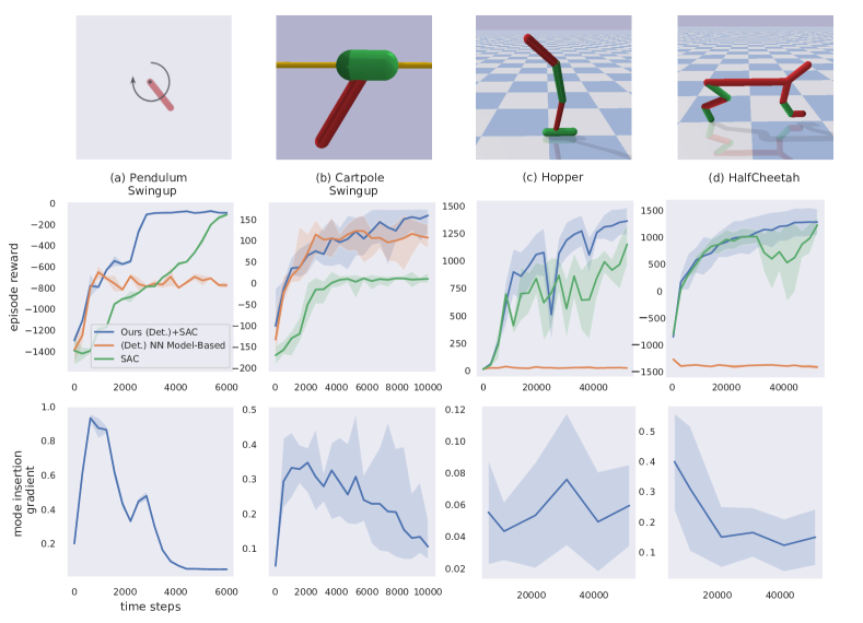
Figure 1: Performance curves of our proposed deterministic hybrid learning algorithm on multiple environments (averaged over 5 random seeds). All methods use the same structured learning models. Our method is shown to improve the model-based benchmark results (due to the use of experience-based methods) while maintaining significant improvements on the number of interactions necessary with the environment to obtain those results. The mode insertion gradient is also shown for each example which illustrates the model-policy agreement over time and the improvement over time.

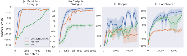
Figure 2: Performance curves of our proposed stochastic hybrid learning algorithm on multiple environments (averaged over 5 random seeds). As shown before, our approach improves both the sample-efficiency but also the highest expected reward. In addition, the stochastic variation of the hybrid learning algorithm generates smoother learning curves as a result of not requiring derivatives of learned models.

Learning from Experience:

We evaluate our approach in the deterministic and stochastic settings using experience-based learning methods and compare against the standard in model-based and experience-based learning. In addition, we illustrate the ability to evaluate our method’s performance of the learned models through the mode insertion gradient. Experimental results validate hybrid learning for real robot tasks. For each example, we use Soft Actor Critic (SAC) [10] as our experience-based method and a neural-network based implementation of model-predictive path integral for reinforcement learning [1] as a benchmark standard method. The parameters for SAC are held as default across all experiments to remove any impact of hyperparameter tuning.

Hybrid learning is tested in four simulated environments: pendulum swingup, cartpole swingup, the hopper environment, and the half-cheetah environment (Fig. 1) using the Pybullet simulator [22]. In addition, we compare against state-of-the-art approaches for model-based and experience-based learning. We first illustrate the results using the deterministic variation of hybrid learning in Fig. 1 (compared against SAC and a deterministic model-predictive controller [23]). Our approach uses the confidence bounds generated by the stochastic policy to infer when best to rely on the policy or predictive models. As a result, hybrid learning allows for performance comparable to experience-based methods with the sample-efficiency of model-based learning approaches. Furthermore, the hybrid control approach allows us to generate a measure for calculating the agreement between the policy and the learned models (bottom plots in Fig. 1), as well as when (and how much) the models were assisting the policy. The commonality between each example is the eventual reduction in the assistance of the learned model and policy. This allows us to better monitor the learning process and dictate how well the policy is performing compared to understanding the underlying task.

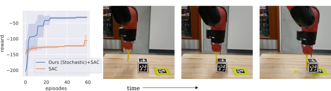
Figure 3: Hybrid learning with experience-based policy results on the Sawyer robot (averaged over 5 trials). The task is to push a block to a designated target through environment interactions (see time-series results above). Our method is able achieve the task within 3 minutes (each episode takes 10 seconds) through effectively using both predictive models and experience-based methods. The same amount of interaction with SAC was unable to successfully push the block to the target.

We next evaluate the stochastic variation of hybrid learning, where we compare against a stochastic neural-network model-based controller [1] and SAC. As shown in Fig. 2, the stochastic variation still maintains the improved performance and sample-efficiency across all examples while also having smoother learning curves. This is a direct result of the derivation of the algorithm where continuity and differentiability of the learned models are not necessary. In addition, exploration is naturally encoded into the algorithm through the policy, which results in more stable learning when there is uncertainty in the task. In contrast, the deterministic approach required added exploration noise to induce exploring other regions of state-space. A similar result is found when comparing the model-based performance of the deterministic and stochastic approaches, where the deterministic variation suffers from modeling discontinuous dynamics.

We can analyze the individual learned model and policy in Fig. 2 obtained from hybrid learning. Specifically, we look at the cartpole swingup task for the stochastic variation of hybrid learning in Fig. 4 and compare against benchmark model-based learning (NN-MPPI [1]) and experience-based learning (SAC [10]) approaches. Hybrid learning is shown to improve the learning capabilities of both the learned predictive model and the policy through the hybrid control approach. In other words, the policy is “filtered” through the learned model and augmented, allowing the robotic system to be guided by both the prediction and experience. Thus, the predictive model and the policy are benefited, ultimately performing better as a standalone approach using hybrid learning.

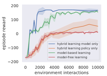
Figure 4: Performance curves for the individual learned model and policy on the cartpole swingup environment during hybrid learning (averaged over 10 trials). Our method is shown to improve the capabilities of the model-based and experience-based components through mutual guidance defined by hybrid control theory. Reference model-based learning (NN-MPPI) and experience-based learning (SAC) approaches are shown for comparison.

Next, we apply hybrid learning on real robot experiments to illustrate the sample-efficiency and performance our approach can obtain (see Fig. 3 for task illustration). We use a Sawyer robot whose goal is to push a block on a table to a specified marker. The position of the marker and the block are known to the robot. The robot is rewarded for pushing the block to the marker. What makes this task difficult is the contact between the arm and the block that the robot needs to discover in order to complete the pushing task. Shown in Fig. 3 our hybrid learning approach is able to learn the task within 20 episodes (total time is 3 minutes, 10 seconds for each episode). Since our method naturally relies on the predictive models when the policy is uncertain, the robot is able to plan through the contact to achieve the task whereas SAC takes significantly longer to discover the pushing dynamics. As a result, we are able to achieve the task with minimal environment interaction.

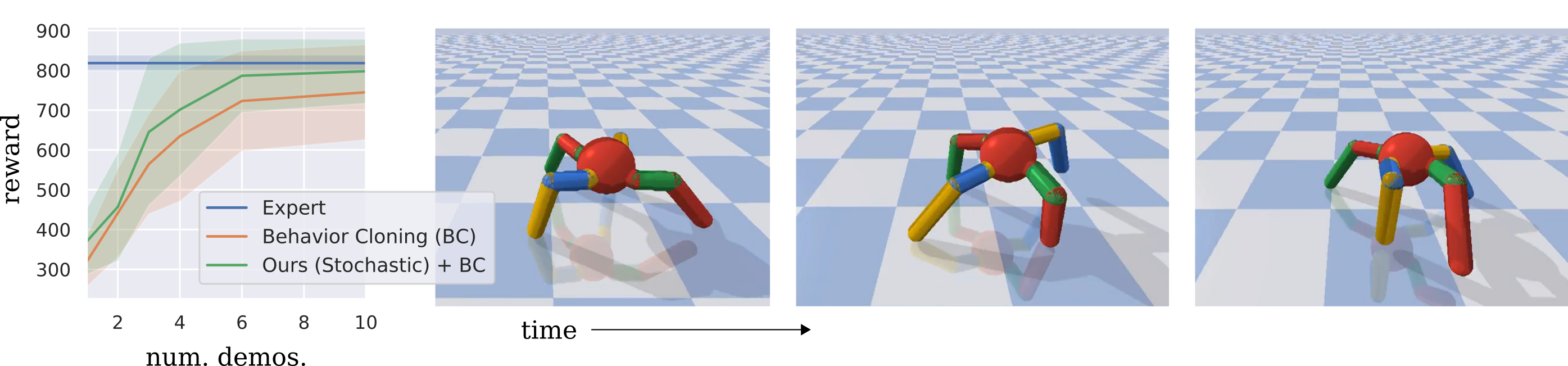
Figure 5: Results for hybrid stochastic control with behavior cloned policies (averaged over 10 trials) using the Ant Pybullet environment (shown in a time-lapsed running sequence). Expert demonstrations (actions executed by an expert policy on the ant robot) are used as experience to boot-strap a learned stochastic policy (behavior cloning) in addition to predictive models which encode the dynamics and the underlying task of the ant. Our method is able to adapt the expert experience to the predictive models, improving the performance of behavior cloning and performing as well as the expert.

Learning from Examples:

We extend our method to use expert demonstrations as experience (also known as imitation learning [24, 25]). Imitation learning focuses on using expert demonstrations to either mimic a task or use as initialization for learning complex data-intensive tasks. We use imitation learning, specifically behavior cloning, as an initialization for how a robot should accomplish a task. Hybrid learning as described in Section 3 is then used as a method to embed model-based information to compensate for the uncertainty in the learned policy, improving the overall performance through planning. The specific algorithmic implementation of hybrid imitation learning is provided in Appendix LABEL:app:imp.

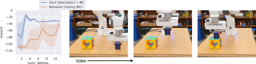
Figure 6: Hybrid learning with behavior cloning results on the Franka panda robot (averaged over 5 trials). The task is to stack a block on top of another using expert demonstrations. Our method is able to learn the block stacking task within three expert demonstrations and provides solutions that are more repeatable than with behavior cloning.

We test hybrid imitation on the Pybullet Ant environment. The goal is for the four legged ant to run as far as it can to the right (from the viewer’s perspective) within the allotted time. At each iteration, we provide the agent with an expert demonstration generated from a PPO [9] solution. Each demonstration is used to construct a predictive model as well as a policy (through behavior cloning). The stochastic hybrid learning approach is used to plan and test the robot’s performance in the environment. Environment experience is then used to update the predictive models while the expert demonstrations are solely used to update the policy. In Fig. 5, we compare hybrid learning against behavior cloning. Our method is able to achieve the task at the level of the expert within 6 (200 step) demonstrations, where the behavior cloned policy is unable to achieve the expert performance. Interestingly, the ant environment is less susceptible to the covariant shift problem (where the state distribution generated by the expert policy does not match the distribution of states generated by the imitated policy [25]), which is common in behavior cloning. This suggests that the ant experiences a significantly large distribution of states during the expert demonstration. However, the resulting performance for the behavior cloning is worse than that of the expert. Our approach is able to achieve similar performance as behavior cloning with roughly 2 fewer demonstrations and performs just as well as the expert demonstrations.

We test our approach on a robot experiment with the Franka Panda robot (which is more likely to have the covariant shift problem). The goal for the robot is to learn how to stack a block on top of another block using demonstrations (see Fig. 6). As with the ant simulated example in Fig. 5, a demonstration is provided at each attempt at the task and is used to update the learned models. Experience obtained in the environment is solely used to update the predictive models. We use a total of ten precollected demonstrations of the block stacking example (given one at a time to the behavior cloning algorithm before testing). At each testing time, the robot arm is initialized at the same spot over the initial block. Since the demonstrations vary around the arm’s initial position, any state drift is a result of the generated imitated actions and will result in the covariant shift problem leading to poor performance. As shown in Fig. 6, our approach is capable of learning the task in as little as two demonstrations where behavior cloning suffers from poor performance. Since our approach synthesizes actions when the policy is uncertain, the robot is able to interpolate between regions where the expert demonstration was lacking, enabling the robot to achieve the task.

5 Conclusion

We present hybrid learning as a method for formally combining model-based learning with experience-based policy learning based on hybrid control theory. Our approach derives the best action a robotic agent can take given the learned models. The proposed method is then shown to improve both the sample-efficiency of the learning process as well as the overall performance of both the model and policy combined and individually. Last, we tested our approach in various simulated and real-world environments using a variety of learning conditions and show that our method improves both the sample-efficiency and the resulting performance of learning motor skills.

References

- Williams et al. [2017] Grady Williams, Nolan Wagener, Brian Goldfain, Paul Drews, James M Rehg, Byron Boots, and Evangelos A Theodorou. Information theoretic MPC for model-based reinforcement learning. In IEEE International Conference on Robotics and Automation, 2017.
- Chua et al. [2018] Kurtland Chua, Roberto Calandra, Rowan McAllister, and Sergey Levine. Deep reinforcement learning in a handful of trials using probabilistic dynamics models. In Advances in Neural Information Processing Systems, pages 4754–4765, 2018.
- Abraham et al. [2020] I. Abraham, A. Handa, N. Ratliff, K. Lowrey, T. D. Murphey, and D. Fox. Model-based generalization under parameter uncertainty using path integral control. IEEE Robotics and Automation Letters, 5(2):2864–2871, 2020.
- Nagabandi et al. [2018] Anusha Nagabandi, Gregory Kahn, Ronald S Fearing, and Sergey Levine. Neural network dynamics for model-based deep reinforcement learning with model-free fine-tuning. In International Conference on Robotics and Automation (ICRA), pages 7559–7566, 2018.
- Havens et al. [2019] Aaron Havens, Yi Ouyang, Prabhat Nagarajan, and Yasuhiro Fujita. Learning latent state spaces for planning through reward prediction. arXiv preprint arXiv:1912.04201, 2019.
- Sharma et al. [2019] Archit Sharma, Shixiang Gu, Sergey Levine, Vikash Kumar, and Karol Hausman. Dynamics-aware unsupervised discovery of skills. arXiv preprint arXiv:1907.01657, 2019.
- Abraham et al. [2017] Ian Abraham, Gerardo de la Torre, and Todd Murphey. Model-based control using koopman operators. In Proceedings of Robotics: Science and Systems, 2017. 10.15607/RSS.2017.XIII.052.
- Abraham and Murphey [2019] Ian Abraham and Todd D Murphey. Active learning of dynamics for data-driven control using koopman operators. IEEE Transactions on Robotics, 35(5):1071–1083, 2019.
- Schulman et al. [2017] John Schulman, Filip Wolski, Prafulla Dhariwal, Alec Radford, and Oleg Klimov. Proximal policy optimization algorithms. arXiv preprint arXiv:1707.06347, 2017.
- Haarnoja et al. [2018] Tuomas Haarnoja, Aurick Zhou, Pieter Abbeel, and Sergey Levine. Soft actor-critic: Off-policy maximum entropy deep reinforcement learning with a stochastic actor. arXiv preprint arXiv:1801.01290, 2018.
- Deisenroth and Rasmussen [2011] Marc Deisenroth and Carl E Rasmussen. PILCO: A model-based and data-efficient approach to policy search. In Proceedings of the 28th International Conference on machine learning (ICML-11), pages 465–472, 2011.
- Pathak et al. [2017] Deepak Pathak, Pulkit Agrawal, Alexei A Efros, and Trevor Darrell. Curiosity-driven exploration by self-supervised prediction. In Conference on Computer Vision and Pattern Recognition Workshops, pages 16–17, 2017.
- Chebotar et al. [2017] Yevgen Chebotar, Mrinal Kalakrishnan, Ali Yahya, Adrian Li, Stefan Schaal, and Sergey Levine. Path integral guided policy search. In International conference on robotics and automation (ICRA), pages 3381–3388, 2017.
- Bansal et al. [2017] Somil Bansal, Roberto Calandra, Kurtland Chua, Sergey Levine, and Claire Tomlin. Mbmf: Model-based priors for model-free reinforcement learning. arXiv preprint arXiv:1709.03153, 2017.
- Levine and Abbeel [2014] Sergey Levine and Pieter Abbeel. Learning neural network policies with guided policy search under unknown dynamics. In Advances in Neural Information Processing Systems, pages 1071–1079, 2014.
- Pomerleau [1998] D Pomerleau. An autonomous land vehicle in a neural network. Advances in neural information processing systems’(Morgan Kaufmann Publishers Inc., 1989), 1, 1998.
- Li and Todorov [2004] Weiwei Li and Emanuel Todorov. Iterative linear quadratic regulator design for nonlinear biological movement systems. In International Conference on Informatics in Control, Automation and Robotics, pages 222–229, 2004.
- Axelsson et al. [2008] Henrik Axelsson, Y Wardi, Magnus Egerstedt, and EI Verriest. Gradient descent approach to optimal mode scheduling in hybrid dynamical systems. Journal of Optimization Theory and Applications, 136(2):167–186, 2008.
- Sutton et al. [2000] Richard S Sutton, David A McAllester, Satinder P Singh, and Yishay Mansour. Policy gradient methods for reinforcement learning with function approximation. In Advances in neural information processing systems, pages 1057–1063, 2000.
- Theodorou and Todorov [2012] Evangelos A Theodorou and Emanuel Todorov. Relative entropy and free energy dualities: Connections to path integral and KL control. In IEEE Conference on Decision and Control (CDC), pages 1466–1473, 2012.
- Williams et al. [2016] Grady Williams, Paul Drews, Brian Goldfain, James M Rehg, and Evangelos A Theodorou. Aggressive driving with model predictive path integral control. In IEEE International Conference on Robotics and Automation, pages 1433–1440, 2016.
- Coumans and Bai [2016] Erwin Coumans and Yunfei Bai. Pybullet, a python module for physics simulation for games, robotics and machine learning. GitHub repository, 2016.
- Ansari and Murphey [2016] Alexander R Ansari and Todd D Murphey. Sequential action control: Closed-form optimal control for nonlinear and nonsmooth systems. IEEE Transactions on Robotics, 32(5):1196–1214, 2016.
- Argall et al. [2009] Brenna D Argall, Sonia Chernova, Manuela Veloso, and Brett Browning. A survey of robot learning from demonstration. Robotics and autonomous systems, 57(5):469–483, 2009.
- Ross and Bagnell [2010] Stéphane Ross and Drew Bagnell. Efficient reductions for imitation learning. In Proceedings of the thirteenth international conference on artificial intelligence and statistics, pages 661–668, 2010.
- Kingma and Ba [2014] Diederik P Kingma and Jimmy Ba. Adam: A method for stochastic optimization. arXiv preprint arXiv:1412.6980, 2014.
- Boyan [1999] Justin A Boyan. Least-squares temporal difference learning. In ICML, pages 49–56, 1999.
- Precup et al. [2001] Doina Precup, Richard S Sutton, and Sanjoy Dasgupta. Off-policy temporal-difference learning with function approximation. In ICML, pages 417–424, 2001.