An Ergodic Measure for Active Learning
From Equilibrium

Abstract

This paper develops KL-Ergodic Exploration from Equilibrium ($\text{KL-E}^{3}$), a method for robotic systems to integrate stability into actively generating informative measurements through ergodic exploration. Ergodic exploration enables robotic systems to indirectly sample from informative spatial distributions globally, avoiding local optima, and without the need to evaluate the derivatives of the distribution against the robot dynamics. Using hybrid systems theory, we derive a controller that allows a robot to exploit equilibrium policies (i.e., policies that solve a task) while allowing the robot to explore and generate informative data using an ergodic measure that can extend to high-dimensional states. We show that our method is able to maintain Lyapunov attractiveness with respect to the equilibrium task while actively generating data for learning tasks such, as Bayesian optimization, model learning, and off-policy reinforcement learning. In each example, we show that our proposed method is capable of generating an informative distribution of data while synthesizing smooth control signals. We illustrate these examples using simulated systems and provide simplification of our method for real-time online learning in robotic systems.

Abstract

Robotic systems need to adapt to sensor measurements and learn to exploit an understanding of the world around them such that they can truly begin to experiment in the real world. Standard learning methods do not have any restrictions on how the robot can explore and learn, making the robot dynamically volatile. Those that do, are often too restrictive in terms of the stability of the robot, resulting in a lack of improved learning due to poor data collection. Applying our method would allow robotic systems to be able to adapt online without the need for human intervention. We show that taking into account both the dynamics of the robot and the statistics of where the robot has been, we are able to naturally encode where the robot needs to explore and collect measurements for efficient learning that is dynamically safe. With our method we are able to effectively learn while being energetically efficient compared to state-of-the-art active learning methods. Our approach accomplishes such tasks in a single execution of the robotic system, i.e., the robot does not need human intervention to reset it. Future work will consider multi-agent robotic systems that actively learn and explore in a team of collaborative robots.

Note to Practitioners:

I Introduction

Robot learning has proven to be a challenge for real-world application. This is partially due to the ineffectiveness of passive data acquisition for learning and the necessity for data-driven actions for collecting informative data. What makes this problem even more difficult is that generating data for robotic systems is often an unstable process. It involves generating measurements dependent upon physical motion of the robot. As a result, safe data collection through exploration becomes a challenge. The problem becomes exacerbated when memory and constraints (i.e., data must come from a single roll out) are imposed on the robot. Thus, robotic systems need to adapt subject to data in a systematic and informative manner while preserving a notion of equilibrium as a means of safety for itself, the environment, and potentially humans. In this paper, we address these issues by developing an algorithm that draws on hybrid systems theory [1] and ergodic exploration [2, 3, 4, 5, 6, 7]. Our approach enables robots to generate and collect informative data while guaranteeing Lyapunov attractiveness [8] with respect to an equilibrium task.

Actively collecting data and learning are often characterized as being part of the same problem of learning from experience [9, 10]. This is generally seen in the field of reinforcement learning (RL) where attempts at a task, as well as learning from the outcome of actions, are used to learn policies and predictive models [9, 11]. Much of the work in the field is dedicated towards generating a sufficiently large distribution of data such that it encompasses unforeseen events, allowing generalization to real-world application [11, 9, 12, 13] however inefficient the method. In this work, rather than trying to generate a large distribution of data given many attempts at a task, we seek to generate an informative data distribution, and learn from the collected distribution of data, as two separate problems, where we focus on actively and intelligently collecting data in a manner that is safe and efficient while adopting existing methods that enable learning.

Current safe learning methods typically provide some bound on the worst outcome model using probabilistic approaches [14], but often only consider the safety with respect to the task and not with respect to the exploration process. We focus on problems where exploring for data intersects with exploring the physical space of robots such that actions that are capable of generating the best set of data can destabilize the robot.

In this work we treat active exploration for data as an ergodic exploration problem, where time spent during the trajectory of the robot is proportional to the measure of informative data in that region. As a result, we are able to efficiently use the physical motion of the robot by focusing on the dynamic area coverage in the search space (as opposed to directly generating samples from the most informative regions). With this approach, we are able to integrate known equilibria and feedback policies (we refer to these as equilibrium policies) which provide attractiveness guarantees—that the robot will eventually return to an equilibrium —while providing the control authority that allows the robot to actively seek out and collect informative data in order to later solve a learning task. Our contributions are summarized as follows:

• Developing a method which extends ergodic exploration to higher dimensional state-spaces using a sample-based measure.

• Synthesis of a control signal that exploits known equilibrium policies.

• Present theoretical results on the Lyapunov attractiveness centered around equilibrium policies of our method.

• Illustrate our method for improving the sample efficiency and quality of data collected for example learning goals.

We structure the paper as follows: Section II provides a list of related work, Section III defines the problem statement for this work. Section IV introduces our approximation to an ergodic metric and Section V formulates the ergodic exploration algorithm for active learning and exploration from equilibrium. Section VI provides examples where our method is applicable. Last, Section VII provides concluding remarks on our method and future directions.

II Related Work

Active Exploration: Existing work generally formulates problems of active exploration as information maximization with respect to a known parameterized model [15, 16]. The problem with this approach is the abundance of local optima [2, 16] which the robotic system needs to overcome, resulting in insufficient data collection. Other approaches have sought to solve this problem by viewing information maximization as an area coverage problem [2, 4]. Ergodic exploration, in particular, has remedied the issue of local optima by using the ergodic metric to minimize the Sobelov distance [17] from the time-averaged statistics of the robot’s trajectory to the expected information in the explored region. This enables both exploration (quickly in low information regions) and exploitation (spending significant amount of time in highly informative regions) in order to avoid local optima and harvest informative measurements. Our work utilizes this concept of ergodicity to improve how robotic systems explore and learn from data.

Ergodicity and Ergodic Exploration: A downside with the current methods for generating ergodic exploration in robots is that they assumes that the model of the robot is fully known. Moreover, there is little guarantee that the robot will not destabilize during the exploration process. This becomes an issue when the robot must explore part of its own state-space (i.e., velocity space) in order to generate informative data. Another issue is that these methods do not scale well with the dimensionality of the search space, making experimental applications with this approach challenging due to computational limitations. Our approach overcomes these issues by using a sample-based KL-divergence measure [4] as a replacement for the ergodic metric. This form of measure has been used previously; however, it relied on motion primitives in order to compute control actions [4]. We show that we can generate a continuous control signal that minimizes this ergodic measure using hybrid systems theory. The same approach is then shown to be readily amenable to existing equilibrium policies. As a result, we can use approximate models of dynamical systems instead of complete dynamic reconstructions in order to actively generate data while ensuring safety in the exploration process through a notion of attractiveness.

Off-Policy Learning: In this work, we utilize concepts from off-policy learning methods [18, 19] which are a set of methods that divides the learning and data generation phases. With these methods, data is first generated using some random policy and a value function is learned from rewards gathered. The value function is then used to create a policy which then updates the value function [20]. Generating more data does not require directly using the policy; however, the most common practice is to use the learned policy with added noise to guide the policy learning. These methods often rely on samples from a buffer of prior data during the training process rather than learning directly through the application of the policy. As such, they are more sample-efficient and can reuse existing data. A disadvantage with off-policy methods is that they are highly dependent on the distribution of data, resulting in an often unstable learning process. Our approach focuses on improving the data generation process through ergodic exploration to generate an informed distribution of data. As a result, the learning process is able to attain improved results from the generated distribution of data and retain its sample-efficiency.

Bayesian Optimization: Our work is most related to the structure of Bayesian optimization [21, 22, 23]. In Bayesian optimization, the goal is to find the maximum of an objective function which is unknown. At each iteration of Bayesian optimization, the unknown objective is sampled and a probabilistic model is generated. An acquisition function is then used as a metric for an “active learner” to find the next best sample. This loop repeats until a maximum is found. In our work, the “active learner” is the robot itself which must abide by the physics that governs its motion. As a result, the assumption that the active learner has the ability to sample anywhere in the search space is lost. Another difference is that instead of using a sample-based method to find the subsequent sampling position, as done in Bayesian optimization, we use ergodic exploration to generate a set of samples proportional to some spatial distribution. We pose the spatial distribution as an acquisition function which we show in Section VI-A. Thus, the active learner is able to sample from regions which have lower probability densities quickly and spending time in regions which are likely to produce an optima. Note that it is possible for one to directly use the derivatives of the acquisition function and a model of the robot’s dynamics to search for the best actions that a robot can take to sample from the objective; however, it is likely that similar issues with information maximization and local optima will occur.

Information Maximization: Last, we review work that addresses the data-inefficiency problem through information maximization [24]. These methods work by either direct maximization of an information measure or by pruning a data-set based on some information measure [25]. These methods still suffer from the problem of local minima due to a lack of exploration or non-convex information objectives [26]. Our work uses ergodicity as a way to gauge how much a robot should be sampling from the exploration space. As a result, the motion of the robot by minimizing an ergodic measure will automatically optimize where and for how long the robot should sample from, avoiding the need to prune from a data-set and sample from multiple highly informative peaks.

The following section introduces ergodicity and ergodic exploration and defines the problem statement for this work.

III Preliminaries: Ergodicity and The Ergodic Metric for Exploration and Exploitation

This section serves as a preliminary section that introduces conceptual background important to the rest of the paper. We first motivate ergodicity as an approach to the exploration vs. exploitation problem and the need for an ergodic measure. Then, we introduce ergodicity and ergodic exploration as the resulting outcome of optimizing an ergodic metric.

The exploration vs. exploitation problem is a problem in robot learning where the robot must deal with the choosing to exploit what it already knows or explore for more information, which entails running the risk of damaging itself or collecting bad data. Ergodic exploration treats the problem of exploration and exploitation as a problem of matching a spatial distributions to a time-averaged distribution—that is, the probability of a positive outcome given a state is directly related to the time spent at that state. Thus, more time is spent in regions where there are positive outcomes (exploitation) and quickly explores states where there is low probability of a positive outcome (exploration).

Definition 1.

Ergodicity, in robotics, is defined when a robot whose time-averaged statistics over its states is equivalent to the spatial statistics of an arbitrarily defined target distribution that intersects those states.

The exact specifications of a spatial statistic varies depending on the underlying task and is defined for different tasks in Sections VI. For now, let us define the time-averaged statistics of a robot by considering its trajectory $x(t):\mathbb{R}\to\mathbb{R}^{n}$ $\forall t\in\left[t_{0},t_{f}\right]$ generated through an arbitrary control process $u(t):\mathbb{R}\to\mathbb{R}^{m}$.

Definition 2.

Given a search domain $\mathcal{S}^{v}\subset\mathbb{R}^{n+m}$ where $v\leq n+m$, the time-averaged statistics (i.e., the time the robot spends in regions of the search domain $\mathcal{S}^{v}$) of a trajectory $x(t)$ is defined as

$$c(s\mid x(t))=\frac{1}{t_{f}-t_{0}}\int_{t_{0}}^{t_{f}}\delta\left[s-\bar{x}(t)\right]dt,$$ (1)

where $s\in\mathcal{S}^{v}$ is a point in the search domain, $\bar{x}(t)$ is the component of the robot’s state $x(t)$ that intersects the search domain, and $\delta[\cdot]$ is the Dirac delta function.

In general, the target spatial statistics are defined through its probability density function $p(s)$ where $p(s)>0$, and $\int_{\mathcal{S}^{v}}p(s)ds=1$. Given a target spatial distribution $p(s)$, we can calculate an ergodic metric as the distance between the Fourier decomposition of $p(s)$ and $c(s\mid x(t))$:

$$\mathcal{E}(x(t))=\sum_{k\in\mathbb{N}^{v}}\Lambda_{k}\left(c_{k}-p_{k}\right)^{2}$$ (2)

where $\Lambda_{k}$ is a weight on the harmonics defined in [27],

$$c_{k} =\frac{1}{t_{f}-t_{0}}\int_{t_{0}}^{t_{f}}F_{k}(x(t))dt,$$

$$p_{k} =\int_{\mathcal{S}^{v}}p(s)F_{k}(s)ds,$$

and $F_{k}(s)$ is the $k^{\text{th}}$ Fourier basis function. Minimizing the ergodic metric results in the time-averaged statistics of $x(t)$ matching the arbitrarily defined target spatial distribution $p(s)$ as well as possible on a finite time horizon and the robotic system sampling measurements in high utility regions specified by $p(s)$.

Figure 1: (a) Illustration of an ergodic trajectory $x(t)$ with respect to (b) target distribution $p(s)$. Time-averaged distribution reconstructions of $x(t)$ are shown using Definitions 2, 3, and Eq. V-C). The Fourier decomposition approach often has residual artifacts due to the cosine approximation. $20$ basis functions are used to approximate the time-averaged distribution. $\Sigma$-approximation to the time-averaged statistics minimizes residual artifacts. (e) Moment matching of the $\Sigma$-approximation provides a simplification for computing the time-averaged statistics.

As in [28, 2], one can calculate a controller that optimizes the ergodic metric such that the trajectory of the robot is ergodic with respect to the distribution $p(s)$ (see Fig 1 for illustration). However, this approach scales $\mathcal{O}(|k|^{n})$ where $|k|$ is the maximum integer–valued Fourier term. As a result, this method is ill-suited for high-dimensional learning tasks whose exploration states are often the full state-space of the robot (often $n>3$ for most mobile robots). Furthermore, the resulting time-averaged distribution reconstruction will often have residual artifacts which require additional conditioning to remove. This motivates the following section which defines an ergodic measure.

IV KL-Divergence Ergodic Measure

As an alternative to computing the ergodic metric, we present an ergodic measure which circumvents the scalability issues mentioned in the previous section. To do this, we utilize the Kullback-–Leibler divergence [29, 30, 4] (KL–divergence) as a measure for ergodicity. Let us first define the approximation to the time-averaged statistics of a trajectory $x(t)$:

Definition 3.

Given a search domain $\mathcal{S}^{v}\subset\mathbb{R}^{n+m}$ the $\Sigma$-approximated time-averaged statistics of the robot is defined by

$$q(s\mid x(t))=\\ \frac{1}{t_{f}-t_{0}}\int_{t_{0}}^{t_{f}}\psi(s\mid x(t))dt$$ (3)

where $\psi(s\mid x(t))=\frac{1}{\eta}\exp\left[-\frac{1}{2}\|s-\bar{x}(t)\|^{2}_{\Sigma^{-1}}\right]$, $\Sigma\in\mathbb{R}^{v\times v}$ is a positive definite matrix parameter that specifies the width of the Gaussian, and $\eta$ is a normalization constant.

We call this an approximation because the true time-averaged statistics, as described in [2] and Definition 2, is a collection of delta functions parameterized by time. We approximate the delta function as a Gaussian distribution with variance $\Sigma$, converging as $\|\Sigma\|\to 0$. As an aside, one can treat $\Sigma$ as a function of $\bar{x}(t)$ if there is uncertainty in the position of the robot.

With this approximation, we are able to relax the ergodic objective in [2] and use the following KL-divergence objective [4]:

$$\footnotesize D_{\text{KL}}(p\|q) =\int_{\mathcal{S}^{v}}p(s)\log\frac{p(s)}{q(s)}ds$$

$$=\int_{\mathcal{S}^{v}}p(s)\log p(s)ds-\int_{\mathcal{S}^{v}}p(s)\log q(s)ds,$$

$$=-\int_{\mathcal{S}^{v}}p(s)\log q(s)ds$$

$$=-\mathbb{E}_{p(s)}\left[\log q(s)\right]$$

where $\mathbb{E}$ is the expectation operator, $q(s)=q(s\mid x(t))$, and $p(s)$ is an arbitrary spatial distribution. Note that we drop the first term in the expanded KL-divergence because it does not depend on the trajectory of the robot $x(t)$. Rather than computing the integral over the exploration space $\mathcal{S}^{v}$ (partly because of intractability), we approximate the expectation operator as

$$D_{\text{KL}}(p\|q) =-\mathbb{E}_{p(s)}\left[\log q(s)\right]$$

$$\approx-\sum_{i=1}^{N}p(s_{i})\log q(s_{i})$$

$$\propto-\sum_{i=1}^{N}p(s_{i})\log\int_{t_{0}}^{t_{f}}\exp\left[-\frac{1}{2}\|s_{i}-\bar{x}(t)\|^{2}_{\Sigma^{-1}}\right]dt,$$ (4)

where $N$ is the number of samples in the search domain drawn uniformly. Through this formulation, we still obtain the benefits of indirectly sampling from the spatial distribution $p(s)$ without having to directly compute derivatives to generate an optimal control signal for the robot. Furthermore, this measure prevents computing the measure from scaling drastically with the number of exploration states. Figure 1 illustrates the resulting reconstruction of the time-averaged statistics of a trajectory $x(t)$ using Definition 3 . The following section uses the KL-divergence ergodic measure and derives a controller which optimizes (IV) while directly incorporating learned models and policies.

V $\text{KL-E}^{3}$: KL-Ergodic Exploration from Equilibrium

In this section, we derive KL-Ergodic Exploration from Equilibrium ($\text{KL-E}^{3}$), which locally optimizes and improves (IV). As an additional constraint, we impose an equilibrium policy and an approximate transition model of the robot’s dynamics on the algorithm. By synthesizing $\text{KL-E}^{3}$ with existing policies that allow the robot to return to an equilibrium state (i.e., local linear quadratic regulators (LQR) controller), we can take advantage of approximate transition models for planning the robot’s motion while providing a bound on how unstable the robot can become. We then show how this method is Lyapunov attractive [31, 32], allowing the robot to become unstable so long as we can ensure the robot will eventually return to an equilibrium.

V-A Model and Policy Assumptions for Equilibrium:

We assume that we have a robot whose approximate dynamics can be modeled using the continuous time transition model:

$$\dot{x}(t) =f(x(t),\mu(x(t)))$$ (5)

$$=g(x(t))+h(x(t))\mu(x(t))$$

where $\dot{x}(t)\in\mathbb{R}^{n}$ is the change of rate of the state $x(t):\mathbb{R}\to\mathbb{R}^{n}$ of the robot at time $t$, $f(x,u):\mathbb{R}^{n\times m}\to\mathbb{R}^{n}$ is the (possibly nonlinear) transition model of the robot as a function of state $x$ and control $u$ which we partition into $g(x):\mathbb{R}^{n}\to\mathbb{R}^{n}$, the free unactuated dynamics, and $h(x):\mathbb{R}^{n}\to\mathbb{R}^{n\times m}$, the actuated dynamics. In our modeling assumption, we consider a policy $\mu(x):\mathbb{R}^{n}\to\mathbb{R}^{m}$ which provides the control signal to the robotic system such that there exists a continuous Lyapunov function $V(x)$ [33, 32] which has the following conditions:

$$V(0)=0$$ (6a)

$$\forall x\in\mathcal{B}\backslash\{0\}\quad V(x)>0$$ (6b)

$$\forall x\in\mathcal{B}\backslash\{0\}\quad \nabla V\cdot f(x,\mu(x))<0$$ (6c)

where $\mathcal{B}\subset\mathbb{R}^{n}$ is a compact and connected set, and

$$\dot{V}(x(t))=\frac{\partial}{\partial x}V(x)\cdot f(x,u)=\nabla V\cdot f(x,u).$$ (7)

Thus, a trajectory $x(t)$ with initial condition at time $t=t_{0}$ subject to (5) and $\mu(x)$ is defined as

$$x(t)=x(t_{0})+\int_{t_{0}}^{t}f(x(t),\mu(x(t)))dt.$$ (8)

For the rest of the paper, we will refer to $\mu(x)$ as an equilibrium policy which is tied to an objective which returns the robot to an equilibrium state. In our prior work [34] we show how one can include any objective into the synthesis of $\text{KL-E}^{3}$.

V-B Synthesizing a Schedule of Exploratory Actions:

Given the assumptions of a known approximate model and an equilibrium policy, our goal is to generate a control signal that augments $\mu(x)$ and minimizes (IV) while ensuring $x$ remains within the compact set $\mathcal{B}$ which will allow the robot to return to an equilibrium state within the time $t\in\left[t_{0},t_{f}\right]$.

Our approach starts by quantifying how sensitive (IV) is to switching from the policy $\mu(x(t))$ to an arbitrary control vector $\mu_{\star}(t)$ at any time $\tau\in\left[t_{0},t_{f}\right]$ for an infinitesimally small duration of time $\lambda$. We will later use this sensitivity to calculate a closed-form solution to the most influential control signal $\mu_{\star}(t)$.

Proposition 1.

The sensitivity of (IV) with respect to the duration time $\lambda$, of switching from the policy $\mu(x)$ to an arbitrary control signal $\mu_{\star}(t)$ at time $\tau$ is

$$\frac{\partial D_{\text{KL}}}{\partial\lambda}=\rho(\tau)^{\top}(f_{2}-f_{1})$$ (9)

where $f_{2}=f(x(\tau),\mu_{\star}(\tau))$ and $f_{1}=f(x(\tau),\mu(x(\tau))$, $\rho(t)\in\mathbb{R}^{n}$ is the adjoint, or co-state variable which is the solution of the following differential equation

$$\dot{\rho}(t)=\sum_{i}\frac{p(s_{i})}{q(s_{i})}\frac{\partial\psi}{\partial x}-\left(\frac{\partial f}{\partial x}+\frac{\partial f}{\partial u}\frac{\partial\mu}{\partial x}\right)^{\top}\rho(t)$$ (10)

subject to the terminal constraint $\rho(t_{f})=\mathbf{0}$, and $\frac{\partial\psi}{\partial x}$ is evaluated at each sample $s_{i}$.

Proof.

See Appendix A ∎

The sensitivity $\frac{\partial}{\partial\lambda}D_{\text{KL}}$ is known as the mode insertion gradient [1]. Note that the second term in (10) encodes how the dynamics will change subject to the policy $\mu(x)$. We can directly compute the mode insertion gradient for any control $\mu_{\star}(t)$ that we choose. However, our goal is to find a schedule of $\mu_{\star}(t)$ which minimizes (IV) while still bounded by the equilibrium policy $\mu(x)$. We solve for this augmented control signal by formulating the following optimization problem:

$$\mu_{\star}(t)=\operatorname*{arg\,min}_{\mu(t)\forall t\in[t_{0},t_{f}]}\int_{t_{0}}^{t_{f}}\frac{\partial}{\partial\lambda}D_{\text{KL}}\Big{|}_{\tau=t}+\frac{1}{2}\|\mu_{\star}(t)-\mu(x(t))\|_{\mathbf{R}}^{2}dt$$ (11)

where $\mathbf{R}\in\mathbb{R}^{m\times m}$ is a positive definite matrix that penalizes the deviation from the policy $\mu(x)$ and $\frac{\partial}{\partial\lambda}D_{\text{KL}}|_{\tau=t}$ is (9) evaluated at time $t$.

Proposition 2.

The augmented control signal $\mu_{\star}(t)$ that minimizes (11) is given by

$$\mu_{\star}(t)=-\mathbf{R}^{-1}h(x(t))^{\top}\rho(t)+\mu(x(t)).$$ (12)

Proof.

Taking the derivative of (11) with respect to $\mu_{\star}(t)$ at each instance in time $t\in[t_{0},t_{f}]$ gives

$$\int_{t_{0}}^{t_{f}}\frac{\partial}{\partial\mu_{\star}} \left(\frac{\partial}{\partial\lambda}D_{\text{KL}}\Big{|}_{\tau=t}+\frac{1}{2}\|\mu_{\star}(t)-\mu(x(t))\|_{\mathbf{R}}^{2}\right)dt$$ (13)

$$=\int_{t_{0}}^{t_{f}}h(x(t))^{\top}\rho(t)+\mathbf{R}(\mu_{\star}(t)-\mu(x(t)))dt$$

where we expand $f(x,u)$ using (5). Since the expression under the integral in (11) is convex in $\mu_{\star}(t)$ and is at an optimizer when (13) is equal to $\mathbf{0}\forall t\in[t_{0},t_{f}]$, we set the expression in (13) to zero and solve for $\mu_{\star}(t)$ at each instant in time giving us

$$\mu_{\star}(t)=-\mathbf{R}^{-1}h(x(t))^{\top}\rho(t)+\mu(x(t))$$

which is the schedule of exploratory actions that reduces the objective for time $t\in\left[t_{0},t_{f}\right]$ and is bounded by $\mu(x)$. ∎

In practice, the first term in (12) is calculated and applied to the robot using a true measurement of the state $\hat{x}(t)$ for the policy $\mu(x)$. We refer to this first term as $\delta\mu_{\star}(t)=-\mathbf{R}^{-1}h(x(t))^{\top}\rho(t)$ yielding $\mu_{\star}(t)=\delta\mu_{\star}(t)+\mu(\hat{x}(t))$.

Given the derivation of the augmented control signal that can generate ergodic exploratory motions, we verify the following through theoretical analysis in the next section:

• that (12) does in fact reduce (IV)

• that (12) imposes a bound on the conditions in (6)

• and that a robotic system subject to (12) has a notion of Lyapunov attractiveness

Theoretical Analysis: We first illustrate that our approach for computing (12) does reduce (IV).

Corollary 1.

Let us assume that $\frac{\partial}{\partial\mu}\mathcal{H}\neq 0$ $\forall t\in\left[t_{0},t_{f}\right]$, where $\mathcal{H}$ is the control Hamiltonian. Then

$$\frac{\partial}{\partial\lambda}D_{\text{KL}}=-\|h(x(t))^{\top}\rho(t)\|_{\mathbf{R}^{-1}}^{2}<0$$ (14)

$\forall t\in\left[t_{0},t_{f}\right]$ subject to $\mu_{\star}(t)$.

Proof.

Inserting (12) into (9) and dropping the dependency of time for clarity gives

$$\frac{\partial}{\partial\lambda}D_{\text{KL}} =\rho(t)^{\top}\left(f_{2}-f_{1}\right)$$

$$=\rho^{\top}\left(g(x)+h(x)\mu_{\star}-g(x)-h(x)\mu(x)\right)$$

$$=\rho^{\top}(-h(x)\mathbf{R}^{-1}h(x)^{\top}\rho+h(x)\mu(x)-h(x)\mu(x))$$

$$=-\rho^{\top}h(x)\mathbf{R}^{-1}h(x)^{\top}\rho$$

$$=-\|h(x(t))^{\top}\rho(t)\|_{\mathbf{R}^{-1}}^{2}\leq 0.$$ (15)

Thus, $\frac{\partial}{\partial\lambda}D_{\text{KL}}$ is always negative subject to (12). ∎

For $\lambda>0$ we can approximate the reduction in $D_{\text{KL}}$ as $\Delta D_{\text{KL}}\approx\frac{\partial}{\partial\lambda}D_{\text{KL}}\lambda\leq 0$. Thus, by applying (12), we are generating exploratory motions that minimize the ergodic measure defined by (IV).

Our next set of analysis involves searching for a bound on the conditions in (6) when (12) is applied at any time $\tau\in\left[0,t-\lambda\right]$ for a duration $\lambda\leq t$.

Theorem 1.

Given the conditions in (6) for a policy $\mu(x)$, then $V(x^{\tau}_{\lambda}(t))-V(x(t))\leq\lambda\beta$, where $x^{\tau}_{\lambda}(t)$ is the solution to (29) subject to (12) for $\tau\in\left[0,t-\lambda\right]$, $\lambda\leq t$, and

$$\beta=\sup_{t\in\left[\tau,\tau+\lambda\right]}-\nabla V\cdot h(x(t))\mathbf{R}^{-1}h(x(t))^{\top}\rho(t).$$ (16)

Proof.

See Appendix A. ∎

We can choose any time $\tau\in\left[0,t-\lambda\right]$ to apply $\mu_{\star}(t)$ and provide an upper bound quantifying the change of the Lyaponov function described in (6) by fixing the maximum value of $\lambda$ during active exploration. In addition, we can tune $\mu_{\star}(t)$ using the regularization value $\mathbf{R}$ such that as $\|\mathbf{R}\|\to\infty$, $\beta\to 0$ and $\mu_{\star}(t)\to\mu(x(t))$.

Given this bound, we can guarantee Lyapunov attractiveness [8], where there exists a time $t$ such that the system (8) is guaranteed to return to a region of attraction (from which the system can be guided towards a stable equilibrium state $x_{0}$).

Definition 4.

A robotic system defined by (5) is Lyapunov attractive if at some time $t$, the trajectory of the system $x(t)\in\mathcal{C}(t)\subset\mathcal{B}$ where $\mathcal{C}(t)=\{x(t)|V(x)\leq\beta^{\star},\nabla V\cdot f(x(t),\mu(x(t)))<0\}$, $\beta^{\star}>0$ is the maximum level set of $V(x)$ where $\nabla V\cdot f(x,\mu(x))<0$, and $\lim_{t\to\infty}x(t)\to x_{0}$ such that $x_{0}$ is an equilibrium state.

Theorem 2.

Given the schedule of exploratory actions (12) $\forall t\in\left[\tau,\tau+\lambda\right]$, a robotic system governed by (5) is Lyapunov attractive such that $\lim_{t\to\infty}x^{\tau}_{\lambda}(t)\to x_{0}$.

Proof.

Using Theorem 1, the integral form of the Lyapunov function (A-B), and the identity (A-B), we can write

$$V(x^{\tau}_{\lambda}(t)) =V(x(0))+\int_{0}^{t}\nabla V\cdot f(x(s),\mu(x(s)))ds$$

$$\quad\quad-\int_{\tau}^{\tau+\lambda}\nabla V\cdot h(x(s))\mathbf{R}^{-1}h(x(s))^{\top}\rho(s)ds$$

$$\leq V(x(0))-\gamma t+\beta\lambda<\beta^{\star},$$

where

$$-\gamma=\sup_{s\in\left[0,t\right]}\nabla V\cdot f(x(s),\mu(x(s)))<0.$$ (17)

Since $\lambda$ is fixed and $\beta$ can be tuned by the matrix weight $\mathbf{R}$, we can choose a $t$ such that $\gamma t\gg\beta\lambda$. Thus, $\lim_{t\to\infty}V(x^{\tau}_{\lambda}(t))\to V(x_{0})$ and $\lim_{t\to\infty}x^{\tau}_{\lambda}(t)\to x_{0}$, implies Lyapunov attractiveness, where $V(x_{0})$ is the minimum of the Lyapunov function at the equilibrium state $x_{0}$.

∎

Proving Lyapunov attractiveness allows us to make the claim that a robot will return to a region where $\dot{V}(x)<0$ subject to the policy $\mu(x)$. This enables the robot to actively explore states which would not naturally have a safe recovery. Moreover, this analysis shows that we can choose the value of $\lambda$ and $\mathbf{R}$ when calculating $\mu_{\star}(t)$ such that attractiveness always holds, giving us an algorithm that is safe for active learning.

So far, we have shown that (12) is a method that generates approximate ergodic exploration from equilibrium policies. We prove that this approach does reduce (IV) and show the ability to quantify and bound how much the active exploration process will deviate the robotic system from equilibrium. Last, it is shown that generating data for learning does not require constant guaranteed Lyapunov stability of the robotic system, but instead introduce the notion of attractiveness where we allow the robot to explore the physical realm so long as the time to explore is finite and the magnitude of the exploratory actions is restrained. In the following section, we extend our previous work in [34] by further approximating the time averaged-statistics so that computing the adjoint variable can be done more efficiently.

V-C $\text{KL-E}^{3}$ for Efficient Planning and Exploration

We extend our initial work by providing a further approximation to computing the time-averaged statistics which improves the computation time of our implementation. Taking note of (IV), we can see that we have to evaluate $q(s_{i})$ at each sample point $s_{i}$ where $q(s)=q(s|x(t))$ has to evaluate the stored trajectory at each time. In real robot experiments, often the underlying spatial statistics $p(s)$ change significantly over time. In addition, most robot experiments require replanning which results in lost information over repeated iterations. Thus, rather than trying to compute the whole time averaged trajectory in Definition 3, we opt to approximate the distribution by applying Jensen’s inequality:

$$q(s|x(t)) \propto\int_{t_{0}}^{t_{f}}\exp\left[-\frac{1}{2}\|s-\bar{x}(t)\|_{\Sigma^{-1}}^{2}\right]dt$$

$$\geq\exp\left(-\frac{1}{2}\int_{t_{0}}^{t_{f}}\|s-\bar{x}(t)\|_{\Sigma^{-1}}^{2}dt\right).$$ (18)

Using this expression in (IV), we can write

$$D_{\text{KL}} \propto-\int_{\mathcal{S}^{v}}p(s)\log q(s)ds$$

$$=-\int_{\mathcal{S}^{v}}p(s)\log\left(\exp\left(-\frac{1}{2}\int_{t_{0}}^{t_{f}}\|s-\bar{x}(t)\|_{\Sigma^{-1}}^{2}dt\right)\right)ds$$

$$\propto\int_{\mathcal{S}^{v}}p(s)\left(\int_{t_{0}}^{t_{f}}\|s-\bar{x}(t)\|_{\Sigma^{-1}}^{2}dt\right)ds$$

$$\approx\sum_{i}^{N}p(s_{i})\int_{t_{0}}^{t_{f}}\|s_{i}-\bar{x}(t)\|_{\Sigma^{-1}}^{2}dt.$$ (19)

Following the results to compute (9), we can show that (12) remains the same where the only modification is in the adjoint differential equation where

$$\dot{\rho}(t)=-\sum_{i}p(s_{i})\frac{\partial\ell}{\partial x}-\left(\frac{\partial f}{\partial x}+\frac{\partial f}{\partial u}\frac{\partial\mu}{\partial x}\right)^{\top}\rho(t)$$ (20)

such that $\ell=\ell(s,x)=\|s-x\|_{\Sigma^{-1}}^{2}$. This formulation has no need to compute $q(s)$ and instead only evaluate $p(s)$ at sampled points. We reserve using this implementation for robotic systems that are of high dimensional space or when calculating the derivatives can be costly due to over-parameterization (i.e., multi-layer networks). Note that all the theoretical analysis still holds because the fundamental theory relies on the construction through hybrid systems theory rather than the KL-divergence itself. The downside to this approach is that one now loses the ability to generate consistent ergodic exploratory movements. The effect can be seen in Figure 1(e) where the trajectory is approximated by a wide Gaussian—rather than the bi-model distribution found in Fig. 1(d). However, for non-stationary $p(s)$, having exact ergodic behavior is not necessary and such approximations at the time-averaged distribution level are sufficient.

In the following subsection, we provide base algorithm and implementation details for $\text{KL-E}^{3}$ and present variations based on the learning goals in VI in the Appendix.

V-D Algorithm Implementation

In this section, we provide an outline of a base implementation of $\text{KL-E}^{3}$ in Algorithm 1. We also define some variables which were not previously mentioned in the derivation of $\text{KL-E}^{3}$ and provide further implementation detail.

There exist many ways one could use (12). For instance, it is possible to simulate a dynamical system for some time horizon $t_{H}$ and apply (12) in a trajectory optimization setting. Another way is to repeatedly generate trajectory plans at each instance and apply the first action in a model-based predictive control (MPC) manner. We found that the choice of $\tau$ and $\lambda$ can determine how one will apply (12). That is, given some time $t_{i}$, if $\tau=t_{i}$ and $\lambda=t_{H}$, we recover the trajectory optimization formulation whereas when $\tau=t_{i}$ and $\lambda=dt$, where $dt$ is the time step, then the MPC formulation is recovered. Rather than focusing on incremental variations, we focus on the general structure of the underlying algorithm when combined with a learning task.

We first assume that we have an approximate transition model $f(x,u)$ and an equilibrium policy $\mu(x)$. A simulation time horizon $t_{H}$ and a time step $dt$ is specified where the true robot measurements of state are given by $\hat{x}(t)$ and the simulated states are $x(t)$. Last, a spatial distribution $p(s)$ is initialized (usually uniform to start), and an empty data set $\mathcal{D}=\{\hat{x}(t_{j}),y(t_{j})\}_{j}$ is initialized where $y(t)$ are measurements.

Constructing $p(s)$ will vary depending on the learning task itself. The only criteria that is necessary for $p(s)$ is that it depends on the measurement data that is collected and used in the learning task. Furthermore, $p(s)$ should represent a utility function that indicates where informative measurements are in the search space to improve the learning task. In the following sections, we provide examples for constructing and updating $p(s)$ given various learning tasks.

Provided the initial items, the algorithm first samples the robot’s state $\hat{x}(t_{i})$ at the current time $t_{i}$. Using the transition model and policy, the next states $x(t)\forall t\in[t_{i},t_{i}+t_{H}]$ are simulated. A set of $N$, samples $(s_{1},s_{2},\ldots,s_{N})$ are generated and used to compute $p(s),q(s)$. The adjoint variable is then backwards simulated from $t=t_{i}+t_{H}\to t_{i}$ and is used to compute $\delta\mu_{\star}(t)$. We ensure robot safety by applying $\delta\mu_{\star}(t)+\mu(\hat{x}(t))$ with real measurements of the robot’s state. Data is then collected and appended to $\mathcal{D}$ and used to update $p(s)$. Any additional steps are specified by the learning task. The pseudo-code for this description is provided in Algorithm 1 .

Algorithm 1 $\text{KL-E}^{3}$ Base Algorithm

1:init: approximate transition model $f(x,u)$, initial true state $\hat{x}(0)$, equilibrium policy $\mu(x)$, spatial distribution $p(s)$, simulation time horizon $t_{H}$, time step $dt$. data set $\mathcal{D}$, $i=0$

2:while task not done do

3:     set $x(t_{i})=\hat{x}(t_{i})$

4:     $\triangleright$ simulation loop

5:     for $\tau_{i}\in\left[t_{i},\ldots,t_{i}+t_{H}\right]$ do

6:           $\triangleright$ forward predict states using any

7:           $\triangleright$ integration method (Euler shown)

8:         $x(\tau_{i+1})=x(\tau_{i})+f(x(\tau_{i}),\mu(x(\tau_{i})))dt$      

9:       $\triangleright$ backwards integrate choosing $\dot{\rho}(t)$

10:       $\triangleright$ set the terminal condition

11:     generate $N$ samples of $s_{i}$ uniformly within $\mathcal{S}^{v}$

12:     $\rho(t_{i}+t_{H})=\mathbf{0}$

13:     for $\tau_{i}\in\left[t_{H}+t_{i},\ldots,t_{i}\right]$ do

14:         $\rho(\tau_{i-1})=\rho(\tau_{i})-\dot{\rho}(\tau_{i})dt$

15:           $\triangleright$ since $x(t)$ is simulated, we return

16:           $\triangleright$ just the first term of (12)

17:           $\triangleright$ and calculate $\mu(x)$ online

18:         $\delta\mu_{\star}(\tau_{i-1})=-\mathbf{R}^{-1}h(x(\tau_{i-1}))^{\top}\rho(\tau_{i-1})$      

19:       $\triangleright$ apply to real robot

20:     chose $\tau\in[t_{i},t_{i}+t_{H}]$ and $\lambda\leq t_{H}$ or use line search [35]

21:     for $t\in[t_{i},t_{i+1}]$ do

22:         if  $t\in[\tau,\tau+\lambda]$ then

23:              apply $\mu_{\star}(t)=\delta\mu_{\star}(t)+\mu(\hat{x}(t))$

24:         else

25:              apply $\mu(x(t))$          

26:         if time to sample then

27:              measure true state $\hat{x}(t)$ and measurements $y(t)$

28:              append to data set $\mathcal{D}\leftarrow\{\hat{x}(t),y(t)\}$               

29:     update $p(s)$ given $\mathcal{D}$ $\triangleright$ task specific

30:     update $f(x,u),\mu(x)$ $\triangleright$ if needed

31:     update learning task

32:     $i\leftarrow i+1$

VI Example Learning Goals

(a) $t=0$

(b) $t=10$

(c) $t=20$

(d) $t=30$

Figure 2: Time series snap-shots of cart double pendulum actively sampling and estimating the objective function (orange). The uncertainty (light blue) calculated from the collected data set drives the exploratory motion of the cart double pendulum while our method ensures that the cart double pendulum is maintained in its upright equilibrium state.

In this section, our goal is to use $\text{KL-E}^{3}$ for improving example methods for learning. In particular, we seek to show that our method can improve Bayesian optimization, transition model learning (also known as dynamics model learning or system identification), and off-policy robot skill learning. In each subsection, we provide an overview of the learning goal and define the spatial distribution $p(s)$ used in our method. In addition, we show the following:

• that our method is capable of improving the learning process through exploration

• that our method does not violate equilibrium policies and destabilize the robot

• and that our method efficiently explores through exploiting the dynamics of a robot and the underlying spatial distribution.

For each example, we provide implementation, including parameters used, in the appendix.

VI-A Bayesian Optimization

In our first example, we explore $\text{KL-E}^{3}$ for Bayesian optimization using a cart double pendulum system [36] that needs to maintain itself at the upright equilibrium. Bayesian optimization is a probabilistic approach for optimizing objective functions $\phi(x):\mathbb{R}^{n}\to\mathbb{R}$ that are either expensive to evaluate or are highly nonlinear. A probabilistic model (often a Gaussian process) of the objective function is built from sampled data $x_{k}\in\mathbb{R}^{n}$ and the posterior of the model is used to construct an acquisition function [22]. The acquisition function maps the sample space $x$ to a value which indicates the utility of the sample (in other words, how likely is the sample to provide information about the objective given the previous sample in $x$). The acquisition function is often simpler and easier to calculate for selecting where to sample next rather than the objective function itself. Assuming one can freely sample the space $x$, Bayesian optimization takes a sample based on the acquisition function and a posterior is computed. The process then repeats until some terminal number of evaluations of the objective or the optimizer is reached. We provide pseudo-code for Bayesian optimization in the Appendix, Alg 2.

In many examples of Bayesian optimization, the assumption is that the learning algorithm can freely sample anywhere in the sample space $x\in\mathbb{R}^{n}$; however, this is not always true. Consider an example where a robot must collect a sample from a Bayesian optimization step where the search space of this sample intersects the state-space of the robot itself. The robot is constrained by its dynamics in terms of how it can sample the objective. Thus, the Bayesian optimization step becomes a constrained optimization problem where the goal is to reach the optimal value of the acquisition function subject to the dynamic constraints of the robot. Furthermore, assume that the motion of the robot is restricted to maintain the robot at an equilibrium (such as maintaining the inverted equilibrium of the cart double pendulum). The problem statement is then to enable a robot to execute a sample step of Bayesian optimization by taking into account the constraints of the robot. We use this example to emphasize the effectiveness of our method for exploiting the local dynamic information using a cart double pendulum where the equilibrium state is at the upright inverted state and a policy maintains the double pendulum upright.

Here, we use a Gaussian process with the radial basis function (RBF) to build a model of the objective function shown in Fig. 2. Using Gaussian process predictive posterior mean $\bar{\mu}(x)$ and variance $\sigma(x)$, the upper confidence bound (UCB) [22] acquisition function is defined as

$$\text{UCB}(x)=\bar{\mu}(x)+\kappa\sigma(x)$$ (21)

where $\kappa>0$. We augment Alg 1 for Bayesian optimization by setting the UCB acquisition function as the target distribution which we define through the Boltzmann softmax function, a common method of converting functions that indicate regions of high-value into distributions [37, 38]:

$$p(s)=\frac{\exp(c\text{UCB}(s))}{\int_{\mathcal{S}^{v}}\exp(c\text{UCB}(\bar{s}))d\bar{s}}$$ (22)

where $c>0$ is a scaling constant. Note that the denominator is approximated as a sum over the samples that our method generates. An approximate linear model of the cart double pendulum dynamics centered around the unstable equilibrium is used along with an LQR policy that maintains the double pendulum upright. We provide brief pseudo-code of the base Algorithm 1 in the Appendix Alg. 3.

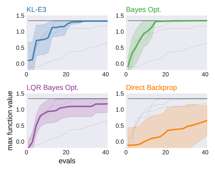
Figure 3: Comparison of $\text{KL-E}^{3}$ against Bayesian Optimization without dynamic constraint, LQR-Bayesian optimization, and direct maximization of the acquisition function through gradient propagation of the cart double pendulum approximate dynamics in determining the maximum value of the objective function through exploration. Our method is able to perform as well as Bayesian optimization directly sampling the exploration space while performing better than the naive LQR-Bayesian optimization. Dashed black line indicates the maximum value of the function.

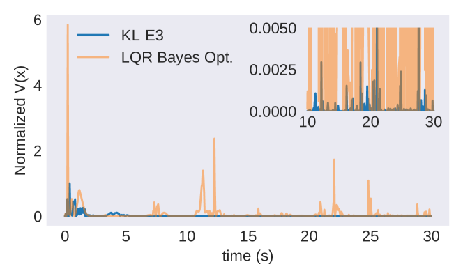
Figure 4: Normalized Lyapunov function for the cart double pendulum with upright equilibrium. Our method (shown in blue) is roughly 6 times more stable than LQR-Bayesian optimization. The large initial values indicate the sweeping shown in Fig. 2(a) when the cart double pendulum moves across the search space. Subsequent application of the exploratory motion refine the exploration process. The Lyapunov attractiveness property is enforced through automatic switching of the exploration process.

We first illustrate that our method generates ergodic exploration through an execution of our method for Bayesian optimization in Figure 2. Here, the time-series evolution of $\text{KL-E}^{3}$ is shown to sample proportional to the acquisition function. As a result, our method generates samples near each of the peaks of the objective function. Furthermore, we can see that our method is exploiting the dynamics as well as the equilibrium policy, maintaining Lyapunov attractiveness with respect to the inverted equilibrium (we will later discuss numerical results in Fig 4).

Next, our method is compared against three variants of Bayesian optimization: the first is Bayesian optimization with no dynamics constraint (i.e., no robot is used); second, a linear quadratic regulator (LQR) variation of Bayesian optimization where the maximum of the acquisition function is used as a target for an LQR controller; and last a direct maximization of the acquisition using the stabilizing equilibrium policy (see [39] for detail) is used. A total of 10 trials for each method are collected with the agent starting at the same location uniformly sampled between $-0.8$ and $0.8$ throughout the sample space. In Fig. 3 we show that our method not only performs comparably to Bayesian optimization without dynamic constraints, but outperforms both LQR and direct maximization variants of Bayesian optimization. Because LQR-Bayes method does not take into account dynamic coverage, and instead focuses on reaching the next sample point, the dynamics of the robot often do not have sufficient time to stabilize which leads to higher variance of the learning objective. We can see this in Fig. 4 where we plot a Lyapunov function for the cart double pendulum [36] at the upright unstable equilibrium. Specifically, our method is roughly 6 times more stable at the start of the exploration compared to the LQR variant of Bayesian optimization. Lyapunov attractiveness is further illustrated in Fig. 4 as time progresses and each exploratory motion is closer to the equilibrium. Last, directly optimizing the highly nonlinear acquisition function often leads to local optima, yielding poor performance in the learning goal. This can be seen with the performance of directly optimizing UCB using the cart double pendulum approximate dynamics in Fig. 3) where the cart double pendulum would often find and settle at a local optima.

In this example, the cart double pendulum only needed to explore the cart position domain to find the maximum of the objective function. The following example illustrates a more dynamic learning goal where the robot needs to generate a stochastic model of its own dynamics through exploration within the state-space.

VI-B Stochastic Transition Model Learning

In this next example $\text{KL-E}^{3}$ is used to collect data for learning a stochastic transition model of a quadcopter [40] dynamical system by exploring the state-space of the quadcopter while remaining at a stable hover. Our goal is to show that our method can efficiently and effectively explore the state-space of the quadcopter (including body linear and angular velocities) in order to generate data for learning a transition model of the quadcopter for model-based control. In addition, we show that the exploratory motions improve the quality of data generated for learning while exploiting and respecting the stable hover equilibrium in a single execution of the robotic system [39].

An LQR policy is used to keep the vehicle hovering while a local linear model (centered around the hover) is used for planning exploratory motions. The stochastic model of the quadcopter is of the form [41]

$$dx\sim\mathcal{N}(f_{\theta}(x,u),\sigma_{\theta}(x))$$ (23)

where $\mathcal{N}$ is a normal distribution with mean $f_{\theta}$, and variance $\sigma_{\theta}(x)$, and the change in the state is given by $dx\in\mathbb{R}^{n}$. Here, $f(x,u;\theta)=f_{\theta}(x,u):\mathbb{R}^{n\times m}\to\mathbb{R}^{n}$ specifies a neural-network model of the dynamics and $\sigma(x;\theta)=\sigma_{\theta}(x)$ is a diagonal Gaussian $\sigma_{\theta}(x):\mathbb{R}^{n}\to\mathbb{R}^{n}$ which defines the uncertainty of the transition model at state $x$ all parameterized by the parameters $\theta$.

We use $\text{KL-E}^{3}$ to enable the quadcopter to explore with respect to the variance of the model (that is, exploration in the state-space is generated based on how uncertain the transition model is at that state). In a similar manner as done in the previous subsection, we use a Boltzmann softmax function to create the distribution

$$p(s)=\frac{\exp(c\sigma_{\theta}(s))}{\int_{\mathcal{S}^{v}}\exp(c\sigma_{\theta}(\bar{s}))d\bar{s}}.$$ (24)

A more complex target distribution can be built (see [42, 39]), however; due to the over-parameterization of the neural-network model, using such methods would require significant computation.

The stochastic model is optimized by maximizing the log likelihood of the model using the likelihood function

$$\mathcal{L}=\mathcal{N}(dx\mid f_{\theta}(x,u),\sigma_{\theta}(x))$$ (25)

where updates to the parameters $\theta$ are defined through the gradient of the log likelihood function:

$$\theta\leftarrow\theta+\alpha\sum_{k}\nabla_{\theta}\log\mathcal{L}.$$ (26)

Here, a batch of $K$ measurements $\{\hat{x}_{k},d\hat{x}_{k},u_{k}\}_{k=1}^{K}$ are uniformly sampled from the data buffer $\mathcal{D}$ where the subscript $k$ denotes the $k^{\text{th}}$ time. A variation of Alg. 1 for model learning is provided in the Appendix in Algorithm 4.

Method	Average Power Loss	Average $\|u\|$
$\text{{KL-E}}^{3}$	0.16 +- 0.0130	0.68 +- 0.0043
Inf. Max*	0.59 +- 0.0463	1.32 +- 0.3075
Normal 0.1*	1.41 +- 0.0121	0.72 +- 0.0016
OU 0.3	2.73 +- 0.0228	1.17 +- 0.0152
OU 0.1	0.97 +- 0.0096	0.73 +- 0.0033
OU 0.01*	0.10 +- 0.0007	0.67 +- 0.0002
Uniform 0.1*	0.84 +- 0.0090	0.69 +- 0.0004

TABLE I: Comparison of our method against various methods for state-space exploration using a quadcopter. Each method uses the same base stabilization policy which maintains hover height and is instantiated and run once for 1200 time steps. Data from a single execution is used to generate a neural network dynamics model. This is repeated $20$ times to estimate the performance of each method. Methods with (*) were unable to generate a dynamics model that completed the tracking objective.

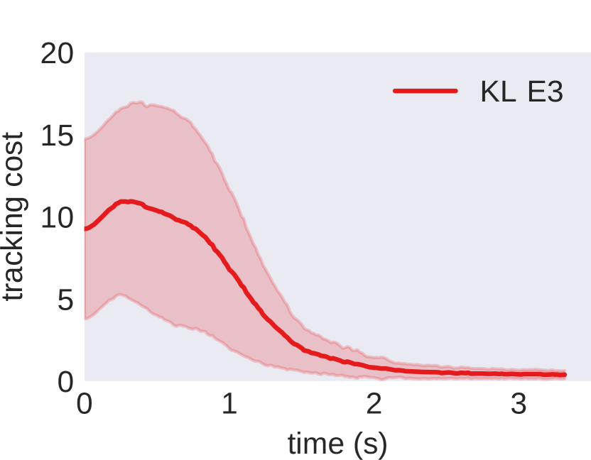
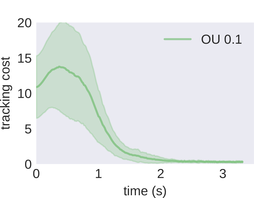
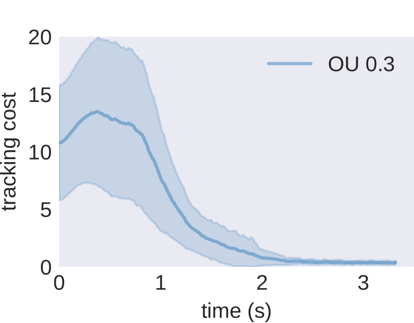
Figure 5: Learned quadcopter model evaluations on a model-based tracking objective. Our method is able to generate a model that performs comparably to OU noise at $0.1$ and $0.3$ noise levels while using less energy through dynamic exploration.

We compare our method against time-correlated Ornstein-Uhlenbeck (OU) noise [43], uniform and normally distributed random noise at different noise levels, and using a nonlinear dynamics variant of the information maximizing method in [39, 42] which directly maximizes the variance of the model subject to the equilibrium policy. Each simulation is run using the LQR controller as a equilibrium policy for a single execution of the robot (no episodic resets) for $1200$ time steps. During this time, data is collected and stored in the buffer $\mathcal{D}$. Our method and the information maximizing method use the data in the stored buffer to update the variance $\sigma_{\theta}(x)$, guiding the exploration process. However, for evaluation of the transition model, we separately learn a model using the data that has been collected as a gauge for the utility of the collected data for each method. A stochastic model is learned by sampling a batch of $200$ measurements offline from the buffer using $2000$ gradient iterations. The model is evaluated for target tracking using stochastic model-based control [44] over a set of uniformly randomly generating target locations $\mathcal{U}(-2,2)\in\mathbb{R}^{3}$.

We first illustrate that our method is more energetically efficient compared to other methods in Table I. Here, energy is calculated using the resulting thrust of the quadcopter and we show the average commanded action $u$ over the execution of the quadrotor in time. Our method is shown to be more energetically efficient (due to the direct exploitation of the equilibrium policy and the ergodic exploration process). Furthermore, our method is able to generate measurements in the state-space that can learn a descriptive stochastic model of the dynamics for model-based tracking control (methods that could not learn a model for tracking control are indicated with a [*]). The resulting methods that could generate a model were comparable to our method (see Fig. 5), however; our method is able to directly target the regions of uncertainty (see Fig. 6) through dynamic exploration allowing the quadcopter to use less energy (and more directed exploratory actions).

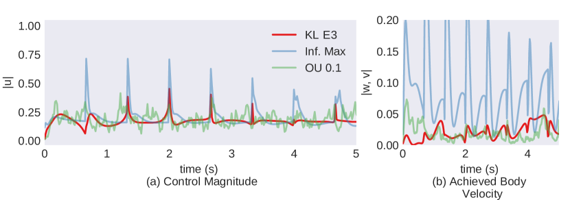
Figure 6: Control signal $\|u(t)\|$ and resulting body linear and angular velocities $\omega,v$ for the quadcopter system using our method, information maximization, and OU noise with $0.1$ maximum noise level. Our method generates smoother control signals while exploring the necessary regions of the state-space without destabilizing the system.

Our last example illustrates how method can be used to aide exploration for off-policy robot skill learning methods by viewing the learned skill as an equilibrium policy.

VI-C Robot Skill Learning

In our last example, we explore $\text{KL-E}^{3}$ for improving robot skill learning (here we consider off-policy reinforcement learning). For all examples, we assume that the learned policy is the equilibrium policy and is simultaneously learned and utilized for safe exploration. As a result, we cannot confirm Lyaponov attractiveness, but assume that the learned policy will eventually yield the Lyaponov property. Thus, our goal is to show that we can consider a robot skill as being in equilibrium (using a feedback policy) where our method can explore within the vicinity of the robot skill in an intentional manner, improving the learning process.

In many examples of robot skill learning, a common mode of failure is that the resulting learned skill is highly dependent on the quality of the distribution of data generated that is used for learning. Typically, these methods use the current iteration of the learned skill (which is often referred to as a policy) with added noise (or have a stochastic policy) to explore the action space. Often the added noise is insufficient towards gaining informative experience which improves the quality of the policy. Here, we show that our method can improve robot skill learning by generating dynamic coverage and exploration around the learned skill, reducing the likelihood of suboptimal solutions, and improving the efficiency of these methods.

We use deep deterministic policy gradient (DDPG) [19] as our choice of off-policy method. Given a set of data, DDPG calculates a Q-function defined as

$$Q(x,u)=\mathbb{E}\left[r(x,u)+\gamma Q(x^{\prime},\mu(x^{\prime}))\right]$$ (27)

where $r(x,u):\mathbb{R}^{n\times m}\to\mathbb{R}$ is a reward function, $x^{\prime}$ is the next state subject to the control $u$, the expectation $\mathbb{E}$ is taken with respect to the states, $0>\gamma>1$ is known as a discounting factor [38], and the function $Q(x,u):\mathbb{R}^{n\times m}\to\mathbb{R}$ maps the utility of a state and how the action at that state will perform in the next state given the policy $\mu(x)$. DDPG simultaneously learns $Q(s)$ and a policy $\mu(x)$ by sampling from a set of collected states, actions, rewards, and their resulting next state. We refer the reader to the pseudo-code of DDPG in [19].

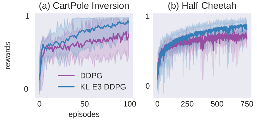
Figure 7: Comparison of $\text{KL-E}^{3}$ enhanced DDPG against DDPG using the cart pole inversion and the half cheetah running tasks. $\text{KL-E}^{3}$ provides a more informative distribution of data which assists the learning process, improves the overall performance, and achieves better performance faster for DDPG.

Our method uses the learned $Q(x,u)$ and $\mu(x)$ as the target distribution and the equilibrium policy respectively. We modify the Q function such that it becomes a distribution using a Boltzmann softmax

$$p(s)=\frac{\exp(cQ(s))}{\int_{\mathcal{S}^{v}}\exp(cQ(\bar{s}))d\bar{s}}$$ (28)

where $s\in\mathbb{R}^{n+m}$ includes both states and actions. This form of Equation (28) has been used previously for inverse reinforcement learning [45, 46]. Here, Eq. (28) is used as a guide for the ergodic exploration where our exploration is centered around the learned policy and the utility of the learned skill (Q-function). Since most reinforcement learning deals with large state-spaces, we use the approximation to the time-averaged statistics in (V-C) to improve the computational efficiency of our algorithm. A parameterized dynamics model is built using the first $200$ points of each simulation (see Appendix for more detail) and updated as each trial continues. OU noise is used for exploration in the DDPG comparison with the same parameters shown in [19]. We provide a pseudo-code of a $\text{KL-E}^{3}$ enhanced DDPG in the Appendix Alg. 5.

Our method is tested on the cart pole inversion and the half-cheetah running task (see Figure 7 for results). For both robotic systems, $\text{KL-E}^{3}$ is shown to improve the overall learning process, making learning a complex robot skill more sample efficient. Specifically, inverting the cart pole starts to occur within $50$ episodes and the half cheetah begins generating running gaits within $250$ episodes of the half cheetah (each episode consists of $200$ time steps of each environment). In contrast, DDPG alone generates suboptimal running (as shown in (https://sites.google.com/view/kle3/home)) and unstable cart inversion attempts. Because our method is able to explore within the vicinity of the learned skill in an intentional, ergodic manner, it is able to quickly learn skills and improve the overall quality of the exploration.

VII Conclusion

We present $\text{KL-E}^{3}$, a method which is shown to enable robots to actively generate informative data for various learning goals from equilibrium policies. Our method synthesizes ergodic coverage using a KL-divergence measure which generates data through exploiting dynamic movement proportional to the utility of the data. We show that hybrid systems theory can be used to synthesize a schedule of exploration actions that can incorporate learned policies and models in a systematic manner. Last, we present examples that illustrate the effectiveness of our method for collecting and generating data in an ergodic manner and provide theoretical analysis which bounds our method through Lyapunov attractiveness.

Appendix A Proofs

A-A Proof of Proposition 1

Proof.

Let us define the trajectory $x(t)$ switching from $\mu(x(\tau))\to\mu_{\star}(\tau)$ for a duration of $\lambda$ as

$$x(t)=x(t_{0}) +\int_{t_{0}}^{\tau}f(x,\mu(x))dt+\int_{\tau}^{\tau+\lambda}f(x,\mu_{\star})dt$$ (29)

$$+\int_{\tau+\lambda}^{t_{f}}f(x,\mu(x))dt$$

where we drop the dependence on time for clarity. Taking the derivative of (IV), using (29), with respect to the duration time $\lambda$ gives us the following expression:

$$\frac{\partial}{\partial\lambda}D_{\text{KL}}=-\sum_{i}\frac{p(s_{i})}{q(s_{i})}\int_{\tau+\lambda}^{t_{f}}\frac{\partial\psi}{\partial x}^{\top}\frac{\partial x}{\partial\lambda}dt.$$ (30)

We obtain $\frac{\partial x}{\partial\lambda}$ by using Leibniz’s rule to evaluate the derivative of (29) with respect to $\lambda$ at the integration boundary conditions to obtain the expression

$$\frac{\partial x(t)}{\partial\lambda}=(f_{2}-f_{1})+\int_{\tau+\lambda}^{t}\left(\frac{\partial f}{\partial x}+\frac{\partial f}{\partial u}\frac{\partial\mu}{\partial x}\right)^{\top}\frac{\partial x(s)}{\partial\lambda}ds$$ (31)

where $s$ is a place holder variable for time, $f_{2}=f(x(\tau+\lambda),\mu_{\star}(\tau+\lambda))$ and $f_{1}=f(x(\tau+\lambda),\mu(x(\tau+\lambda))$. Noting that $\frac{\partial x}{\partial\lambda}$ is a repeated term under the integral, (31) is a linear convolution with initial condition $\frac{\partial x(\tau+\lambda)}{\partial\lambda}=f_{2}-f_{1}$. As a result, we can rewrite (31) using a state-transition matrix [47]

$$\Phi(t,\tau+\lambda)=\exp\left(\left(\frac{\partial f}{\partial x}+\frac{\partial f}{\partial u}\frac{\partial\mu}{\partial x}\right)^{\top}\left(t-\tau\right)\right)$$

with initial condition $f_{2}-f_{1}$ as

$$\frac{\partial x(t)}{\partial\lambda}=\Phi(t,\tau+\lambda)(f_{2}-f_{1}).$$ (32)

Using (32) in (30) gives the following expression

$$\frac{\partial}{\partial\lambda}D_{\text{KL}}=-\sum_{i}\frac{p(s_{i})}{q(s_{i})}\int_{\tau+\lambda}^{t_{f}}\frac{\partial\psi}{\partial x}^{\top}\Phi(t,\tau+\lambda)dt\left(f_{2}-f_{1}\right).$$ (33)

Taking the limit as $\lambda\to 0$ we then set

$$\rho(\tau)^{\top}=-\sum_{i}\frac{p(s_{i})}{q(s_{i})}\int_{\tau}^{t_{f}}\frac{\partial\psi}{\partial x}^{\top}\Phi(t,\tau)dt$$ (34)

in (33) which results in

$$\frac{\partial}{\partial\lambda}D_{\text{KL}}=\rho(\tau)^{\top}\left(f_{2}-f_{1}\right).$$ (35)

Taking the derivative of (34) with respect to time $\tau$ yields the following:

$$\frac{\partial}{\partial\tau}\rho(\tau)^{\top}=\sum_{i}\frac{p(s_{i})}{q(s_{i})}\frac{\partial\psi}{\partial x}^{\top}\Phi(\tau,\tau)\\ -\sum_{i}\frac{p(s_{i})}{q(s_{i})}\int_{\tau}^{t_{f}}\frac{\partial\psi}{\partial x}^{\top}\frac{\partial}{\partial\tau}\Phi(t,\tau)dt.$$

Since $\Phi(\tau,\tau)=1$, and

$$\frac{\partial}{\partial\tau}\Phi(t,\tau)=-\Phi(t,\tau)\left(\frac{\partial f}{\partial x}+\frac{\partial f}{\partial u}\frac{\partial\mu}{\partial x}\right),$$

we can show that

$$\frac{\partial}{\partial\tau}\rho(\tau)^{\top}=\sum_{i}\frac{p(s_{i})}{q(s_{i})}\frac{\partial\psi}{\partial x}^{\top}\\ -\underbrace{\left(-\sum_{i}\frac{p(s_{i})}{q(s_{i})}\int_{\tau}^{t_{f}}\frac{\partial\psi}{\partial x}^{\top}\Phi(t,\tau)dt\right)}_{=\rho(\tau)^{\top}}\left(\frac{\partial f}{\partial x}+\frac{\partial f}{\partial u}\frac{\partial\mu}{\partial x}\right).$$

Taking the transpose, we can show that $\rho(t)$ can be solved backwards in time with the differential equation

$$\dot{\rho}(t)=\sum_{i}\frac{p(s_{i})}{q(s_{i})}\frac{\partial\psi}{\partial x}-\left(\frac{\partial f}{\partial x}+\frac{\partial f}{\partial u}\frac{\partial\mu}{\partial x}\right)^{\top}\rho(t)$$ (36)

with final condition $\rho(t_{f})=\mathbf{0}$. ∎

A-B Proof of Theorem 1

Proof.

Writing the integral form of the Lyapunov function switching between $\mu(x(t))$ and $\mu_{\star}(t)$ at time $\tau$ for a duration of time $\lambda$ starting at $x(0)$ can be written as

$$V(x^{\tau}_{\lambda}(t))=V(x(0))+ \int_{0}^{\tau}\nabla V\cdot f(x(s),\mu(x(s)))ds$$

$$+ \int_{\tau}^{\tau+\lambda}\nabla V\cdot f(x(s),\mu_{\star}(s))ds$$

$$+ \int_{\tau+\lambda}^{t}\nabla V\cdot f(x(s),\mu(x(s)))ds$$ (37)

where $s$ is a place holder for time. Expanding $f(x,u)$ to $g(x)+h(x)u$ and using (12) we can show the following identity:

$$\nabla V\cdot f(x,\mu_{\star}) =\nabla V\cdot g(x)+\nabla V\cdot h(x)\mu_{\star}$$

$$=\nabla V\cdot g(x)+\nabla V\cdot h(x)\mu(x)$$

$$\qquad\qquad-\nabla V\cdot h(x)\mathbf{R}^{-1}h(x)^{\top}\rho$$

$$=\nabla V\cdot f(x,\mu(x))-\nabla V\cdot h(x)\mathbf{R}^{-1}h(x)^{\top}\rho$$ (38)

Using (A-B) in (A-B), we can show that

$$V(x^{\tau}_{\lambda}(t)) =V(x(0))+\int_{0}^{t}\nabla V\cdot f(x(s),\mu(x(s)))ds$$

$$\quad\quad-\int_{\tau}^{\tau+\lambda}\nabla V\cdot h(x(s))\mathbf{R}^{-1}h(x(s))^{\top}\rho(s)ds$$

$$=V(x(t))$$

$$\quad\quad-\int_{\tau}^{\tau+\lambda}\nabla V\cdot h(x(s))\mathbf{R}^{-1}h(x(s))^{\top}\rho(s)ds$$ (39)

where $x(t)$ is given by (8).

Letting the largest value of $\nabla V\cdot h(x(t))\mathbf{R}^{-1}h(x(t))^{\top}\rho(t)$ be given by

$$\beta=\sup_{s\in\left[\tau,\tau+\lambda\right]}-\nabla V\cdot h(x(s))\mathbf{R}^{-1}h(x(s))^{\top}\rho(s)>0,$$ (40)

we can approximate (A-B) as

$$V(x^{\tau}_{\lambda}(t)) =V(x(t))-\int_{\tau}^{\tau+\lambda}\nabla V\cdot h(x(s))\mathbf{R}^{-1}h(x(s))^{\top}\rho(s)ds$$

$$\leq V(x(t))+\beta\lambda.$$

Subtracting both side by $V(x(t))$ gives the upper bound

$$V(x^{\tau}_{\lambda}(t))-V(x(t))\leq\beta\lambda$$ (41)

which quantifies how much (12) deviates from the equilibrium conditions in (6). ∎

Appendix B Algorithmic Details

This appendix provides additional details for each learning goal presented in Section VI. This includes pseudo-code for each method and parameters to implement our examples (see Table. II). We provide videos of each example and demo code in (https://sites.google.com/view/kle3/home).

Example	$t_{H}$	$\lambda$	$f(x,u)$	$\mu(x)$	$\mathbf{R}$	$\Sigma$	$N$ samples
Cart Double Pendulum Bayes. Opt.	0.2 s	line search $\lambda<t_{H}$	local linear model at inverted pose	LQR stabilizing policy	0.1	0.1	20
Quadcopter Model Learning	0.6 s	$\lambda=t_{H}$	local linear model at hoverheight	LQR hovering policy	$0.5\mathbf{I}$	$0.1\mathbf{I}$	100
DDPG Cart pole swingup	0.1 s	$\lambda=0.02$ s	neural-net model $\dot{x}=f(x,u;\theta)$ learned from data	Learned swingup skill	$0.01*0.99^{t}$	$0.1\mathbf{I}$	20
DDPG Half Cheetah running	0.03 s	$\lambda=0.0165s$	neural-net model $\dot{x}=f(x,u;\theta)$ learned from data	Learned running skill	$0.01*0.99^{t}$	$0.1\mathbf{I}$	50

TABLE II: Parameters used for each method presented in Section VI . $\mathbf{I}$ indicates an identity matrix of size $m\times m$, $n\times n$ for the quadcopter model learning, and $v\times v$ where $v=n+m$ used in both DDPG examples. Neural net model parameters $\theta$ are learned by minimizing the error $\|\dot{x}-f(x,u;\theta)\|^{2}$ over a subset of $K$ data points where $\dot{x}\approx(x(t_{1})-x(t_{0}))/dt$ and $dt$ is the time step of the system. A time-decaying $\mathbf{R}$ is used for both DDPG examples so that the largest exploring occurs earlier on in the episode to better assist the skill learning.

Algorithm 2 Bayesian Optimization

1:init: Gaussian prior on objective $\phi$, data set $\mathcal{D}$, $i=0$

2:while task not done do

3:     update posterior distribution on $\phi$ using $\mathcal{D}$

4:     build acquisition function using current posterior on $\phi$

5:     active learner finds the maximum $x_{i}$ of the acquisition function

6:     active learner samples $y_{i}=\phi(x_{i})$

7:     $i\leftarrow i+1$

8:     set $x(t_{i})=\hat{x}(t_{i})$

9:return max $y_{i}$ of $\phi(x)$ and argmax $x_{i}$

Algorithm 3 $\text{KL-E}^{3}$ for Bayesian Optimization

1:init: see Alg. 1 and Alg. 2

2:while task not done do

3:     set $x(t_{i})=\hat{x}(t_{i})$

4:     $\triangleright$ simulation loop (see Alg. 1 lines 4-18)

5:     get $\delta\mu(t)$ from simulation

6:     $\triangleright$ apply to real robot (see Alg. 1 lines 20-28)

7:     chose $\tau\in[t_{i},t_{i}+t_{H}]$ and $\lambda\leq t_{H}$

8:     $\triangleright$

9:     for $t\in[t_{i},t_{i+1}]$ do

10:         if  $t\in[\tau,\tau+\lambda]$ then

11:              apply $\mu_{\star}(t)=\delta\mu_{\star}(t)+\mu(\hat{x}(t))$

12:         else

13:              apply $\mu(x(t))$          

14:         if time to sample then

15:              measure true state $\hat{x}(t)$ and $y(t)=\phi(\hat{x}(t))$

16:              append to data set $\mathcal{D}\leftarrow\{\hat{x}(t),y(t)\}$               

17:     update posterior on $\phi$ given $\mathcal{D}$

18:     update $p(s)$ from posterior

19:     $i\leftarrow i+1$

Algorithm 4 $\text{KL-E}^{3}$ for Model Learning

1:init: see Alg. 1, generate initial parameter $\theta^{0}$ for model (23)

2:while task not done do

3:     set $x(t_{i})=\hat{x}(t_{i})$

4:     $\triangleright$ simulation loop (see Alg. 1 lines 4-18)

5:     get $\delta\mu(t)$ from simulation

6:     $\triangleright$ apply to real robot

7:     chose $\tau\in[t_{i},t_{i}+t_{H}]$ and $\lambda\leq t_{H}$

8:     for $t\in[t_{i},t_{i+1}]$ do

9:         if  $t\in[\tau,\tau+\lambda]$ then

10:              apply $\mu_{\star}(t)=\delta\mu_{\star}(t)+\mu(\hat{x}(t))$

11:         else

12:              apply $\mu(x(t))$          

13:         if time to sample then

14:              measure state $\hat{x}(t)$, change in state $d\hat{x}(t)$, and applied control $u(t)$

15:              append to data set $\mathcal{D}\leftarrow\{\hat{x}(t),d\hat{x}(t),u(t)\}$               

16:     sample $K$ batch $\{\hat{x}_{k},d\hat{x}_{k},u_{k}\}_{k=1}^{K}$

17:     $\theta^{i+1}\leftarrow\theta^{i}+\sum_{k}\nabla_{\theta}\log\mathcal{L}$ given batch

18:     update $p(s)$ from $\sigma_{\theta^{i+1}}$

19:     $i\leftarrow i+1$

Algorithm 5 $\text{KL-E}^{3}$ enhanced DDPG

1:init: see Alg. 1,  [19],

2:while task not done do

3:     set $x(t_{i})=\hat{x}(t_{i})$

4:     $\triangleright$ simulation loop (see Alg. 1 lines 4-18)

5:     get $\delta\mu(t)$ from simulation and apply to real robot

6:     chose $\tau\in[t_{i},t_{i}+t_{H}]$ and $\lambda\leq t_{H}$

7:     for $t\in[t_{i},t_{i+1}]$ do

8:         if  $t\in[\tau,\tau+\lambda]$ then

9:              apply $\mu_{\star}(t)=\delta\mu_{\star}(t)+\mu(\hat{x}(t))$

10:         else

11:              apply $\mu(x(t))$          

12:         if time to sample then

13:              measure state $\hat{x}(t)$, next state $\hat{x}^{\prime}(t)$, applied control $u(t)$, reward $r(t)$

14:              append $\mathcal{D}\leftarrow\{\hat{x}(t),\hat{x}^{\prime}(t),u(t),r(t)\}$               

15:     if time to update and buffer is large enough then

16:         update $Q$, $\mu$ from  [19]

17:         update $p(s)$ using $Q$ (28)      

18:     $i\leftarrow i+1$

Ian Abraham Ian Abraham received the B.S. degree in Mechanical and Aerospace Engineering from Rutgers University and the M.S. degree in Mechanical Engineering from Northwestern University. He is currently a Ph.D. Candidate at the Center for Robotics and Biosystems at Northwestern University. His Ph.D. work focuses on developing formal methods for robot sensing and runtime active learning. He is also the recipient of the 2019 King-Sun Fu IEEE Transactions on Robotics Best Paper award.

Ahalya Prabhakar Ahalya Prabhakar received the B.S. degree in mechanical engineering from California Institute of Technology, Pasadena, CA, USA, in 2013, and the M.S. degree in mechanical engineering from Northwestern University, Evanston, IL, USA, in 2016. She is a Ph.D. candidate at the Center for Robotics and Biosystems at Northwestern University. Her work focuses on developing compressible representations through active exploration for complex task performance and efficient robot learning.

Todd D. Murphey Todd D. Murphey received his B.S. degree in mathematics from the University of Arizona and the Ph.D. degree in Control and Dynamical Systems from the California Institute of Technology. He is a Professor of Mechanical Engineering at Northwestern University. His laboratory is part of the Neuroscience and Robotics Laboratory, and his research interests include robotics, control, computational methods for biomechanical systems, and computational neuroscience. Honors include the National Science Foundation CAREER award in 2006, membership in the 2014-2015 DARPA/IDA Defense Science Study Group, and Northwestern’s Professorship of Teaching Excellence. He was a Senior Editor of the IEEE Transactions on Robotics.

References

- [1] H. Axelsson, Y. Wardi, M. Egerstedt, and E. Verriest, “Gradient descent approach to optimal mode scheduling in hybrid dynamical systems,” Journal of Optimization Theory and Applications, vol. 136, no. 2, pp. 167–186, 2008.
- [2] L. M. Miller, Y. Silverman, M. A. MacIver, and T. D. Murphey, “Ergodic exploration of distributed information,” IEEE Transactions on Robotics, vol. 32, no. 1, pp. 36–52, 2016.
- [3] A. Mavrommati, E. Tzorakoleftherakis, I. Abraham, and T. D. Murphey, “Real-time area coverage and target localization using receding-horizon ergodic exploration,” IEEE Transactions on Robotics, vol. 34, no. 1, pp. 62–80, 2018.
- [4] E. Ayvali, H. Salman, and H. Choset, “Ergodic coverage in constrained environments using stochastic trajectory optimization,” in International Conference on Intelligent Robots and Systems, 2017, pp. 5204–5210.
- [5] I. Abraham, A. Prabhakar, M. J. Hartmann, and T. D. Murphey, “Ergodic exploration using binary sensing for nonparametric shape estimation,” IEEE robotics and automation letters, vol. 2, no. 2, pp. 827–834, 2017.
- [6] I. Abraham, A. Mavrommati, and T. D. Murphey, “Data-driven measurement models for active localization in sparse environments,” in Robotics: Science and Systems, 2018.
- [7] I. Abraham and T. D. Murphey, “Decentralized ergodic control: distribution-driven sensing and exploration for multiagent systems,” IEEE Robotics and Automation Letters, vol. 3, no. 4, pp. 2987–2994, 2018.
- [8] A. Polyakov and L. Fridman, “Stability notions and Lyapunov functions for sliding mode control systems,” Journal of the Franklin Institute, vol. 351, no. 4, pp. 1831–1865, 2014.
- [9] P. Kormushev, S. Calinon, and D. G. Caldwell, “Robot motor skill coordination with EM-based reinforcement learning,” in International Conference on Intelligent Robots and Systems, 2010, pp. 3232–3237.
- [10] R. F. Reinhart, “Autonomous exploration of motor skills by skill babbling,” Autonomous Robots, vol. 41, no. 7, pp. 1521–1537, 2017.
- [11] C. D. McKinnon and A. P. Schoellig, “Learning multimodal models for robot dynamics online with a mixture of Gaussian process experts,” in International Conference on Robotics and Automation, 2017, pp. 322–328.
- [12] J. Tan, T. Zhang, E. Coumans, A. Iscen, Y. Bai, D. Hafner, S. Bohez, and V. Vanhoucke, “Sim-to-real: Learning agile locomotion for quadruped robots,” in Proceedings of Robotics: Science and Systems, 2018.
- [13] A. Marco, F. Berkenkamp, P. Hennig, A. P. Schoellig, A. Krause, S. Schaal, and S. Trimpe, “Virtual vs. real: Trading off simulations and physical experiments in reinforcement learning with Bayesian optimization,” in International Conference on Robotics and Automation, 2017, pp. 1557–1563.
- [14] F. Berkenkamp, M. Turchetta, A. Schoellig, and A. Krause, “Safe model-based reinforcement learning with stability guarantees,” in Advances in Neural Information Processing Systems, 2017, pp. 908–918.
- [15] T.-C. Lin and Y.-C. Liu, “Direct learning coverage control based on expectation maximization in wireless sensor and robot network,” in Conference on Control Technology and Applications, 2017, pp. 1784–1790.
- [16] F. Bourgault, A. A. Makarenko, S. B. Williams, B. Grocholsky, and H. F. Durrant-Whyte, “Information based adaptive robotic exploration,” in International Conference on Intelligent Robots and Systems, vol. 1, 2002, pp. 540–545.
- [17] R. Arnold and A. Wellerding, “On the sobolev distance of convex bodies,” aequationes mathematicae, vol. 44, no. 1, pp. 72–83, 1992.
- [18] D. Precup, R. S. Sutton, and S. Dasgupta, “Off-policy temporal-difference learning with function approximation,” in ICML, 2001, pp. 417–424.
- [19] T. P. Lillicrap, J. J. Hunt, A. Pritzel, N. Heess, T. Erez, Y. Tassa, D. Silver, and D. Wierstra, “Continuous control with deep reinforcement learning,” arXiv preprint arXiv:1509.02971, 2015.
- [20] L. P. Kaelbling, M. L. Littman, and A. W. Moore, “Reinforcement learning: A survey,” Journal of artificial intelligence research, vol. 4, pp. 237–285, 1996.
- [21] P. I. Frazier, “A tutorial on Bayesian optimization,” arXiv preprint arXiv:1807.02811, 2018.
- [22] J. Snoek, H. Larochelle, and R. P. Adams, “Practical Bayesian optimization of machine learning algorithms,” in Advances in neural information processing systems, 2012, pp. 2951–2959.
- [23] R. Calandra, A. Seyfarth, J. Peters, and M. P. Deisenroth, “Bayesian optimization for learning gaits under uncertainty,” Annals of Mathematics and Artificial Intelligence, vol. 76, no. 1-2, pp. 5–23, 2016.
- [24] M. Schwager, P. Dames, D. Rus, and V. Kumar, “A multi-robot control policy for information gathering in the presence of unknown hazards,” in Robotics research, 2017, pp. 455–472.
- [25] D. Nguyen-Tuong and J. Peters, “Incremental online sparsification for model learning in real-time robot control,” Neurocomputing, vol. 74, no. 11, pp. 1859–1867, 2011.
- [26] D. Ucinski, Optimal measurement methods for distributed parameter system identification. CRC Press, 2004.
- [27] G. Mathew and I. Mezić, “Metrics for ergodicity and design of ergodic dynamics for multi-agent systems,” Physica D: Nonlinear Phenomena, vol. 240, no. 4-5, pp. 432–442, 2011.
- [28] L. M. Miller and T. D. Murphey, “Trajectory optimization for continuous ergodic exploration,” in 2013 American Control Conference, 2013, pp. 4196–4201.
- [29] S. Kullback and R. A. Leibler, “On information and sufficiency,” The annals of mathematical statistics, vol. 22, no. 1, pp. 79–86, 1951.
- [30] S. Kullback, Information theory and statistics. Courier Corporation, 1997.
- [31] E. D. Sontag, “Control-Lyapunov functions,” in Open problems in mathematical systems and control theory, 1999, pp. 211–216.
- [32] S. M. Khansari-Zadeh and A. Billard, “Learning control Lyapunov function to ensure stability of dynamical system-based robot reaching motions,” Robotics and Autonomous Systems, vol. 62, no. 6, pp. 752–765, 2014.
- [33] Z. Artstein, “Stabilization with relaxed controls,” Nonlinear Analysis: Theory, Methods & Applications, vol. 7, no. 11, pp. 1163–1173, 1983.
- [34] I. Abraham, A. Prabhakar, and T. D. Murphey, “Active area coverage from equilibrium,” in Workshop on Algorithmic Foundations of Robotics, 2019.
- [35] J. J. Moré and D. J. Thuente, “Line search algorithms with guaranteed sufficient decrease,” ACM Transactions on Mathematical Software (TOMS), vol. 20, no. 3, pp. 286–307, 1994.
- [36] W. Zhong and H. Rock, “Energy and passivity based control of the double inverted pendulum on a cart,” in IEEE International Conference on Control Applications, 2001, pp. 896–901.
- [37] C. M. Bishop, Pattern recognition and machine learning. Springer, 2006.
- [38] R. S. Sutton and A. G. Barto, Reinforcement learning: An introduction. MIT press, 2018.
- [39] I. Abraham and T. D. Murphey, “Active learning of dynamics for data-driven control using koopman operators,” IEEE Transactions on Robotics, vol. 35, no. 5, pp. 1071–1083, 2019.
- [40] T. Fan and T. Murphey, “Online feedback control for input-saturated robotic systems on lie groups,” arXiv preprint arXiv:1709.00376, 2017.
- [41] Y. Gal, R. McAllister, and C. E. Rasmussen, “Improving pilco with Bayesian neural network dynamics models,” in Data-Efficient Machine Learning workshop, ICML, vol. 4, 2016.
- [42] A. D. Wilson, J. A. Schultz, A. R. Ansari, and T. D. Murphey, “Dynamic task execution using active parameter identification with the baxter research robot,” Transactions on Automation Science and Engineering, vol. 14, no. 1, pp. 391–397, 2017.
- [43] G. E. Uhlenbeck and L. S. Ornstein, “On the theory of the brownian motion,” Physical review, vol. 36, no. 5, p. 823, 1930.
- [44] G. Williams, P. Drews, B. Goldfain, J. M. Rehg, and E. A. Theodorou, “Aggressive driving with model predictive path integral control,” in IEEE International Conference on Robotics and Automation (ICRA), 2016, pp. 1433–1440.
- [45] E. Bıyık and D. Sadigh, “Batch active preference-based learning of reward functions,” arXiv preprint arXiv:1810.04303, 2018.
- [46] D. S. Brown, Y. Cui, and S. Niekum, “Risk-aware active inverse reinforcement learning,” arXiv preprint arXiv:1901.02161, 2019.
- [47] B. D. Anderson and J. B. Moore, Optimal control: linear quadratic methods. Courier Corporation, 2007.