Quantum Optics of an Oscillator Falling into a Black Hole

Abstract

We present a quantum optics treatment of the near horizon behaviour of a quantum oscillator freely-falling into a pre-existing Schwarzschild black hole. We use Painlevé-Gullstrand coordinates to define a global vacuum state. In contrast to an accelerated oscillator in the Minkowski vacuum, where there is no radiation beyond an initial transient, we find that the oscillator radiates positive energy to to infinity and negative energy into the black hole as it attempts to come into equilibrium with the ambient vacuum. We discuss the relationship of the model to Hawking radiation.

1 Introduction

Hawking’s original paper [11] showed that when quantum effects are considered, black holes radiate a thermal flux of particles. Despite multiple derivations the physical understanding of Hawking radiation is far from complete with a number of proposed mechanisms include tidal forces on virtual particle-anti-particle pairs analogous to pair creation in an electric field, the splitting of entangled modes as the horizon forms, and quantum tunnelling through the horizon[3] [10].

Since the Hawking radiation is in a sense universal, independent of details of the collapse phase of matter in the formation of the black hole, it should be possible to understand some of its features by constructing physical models. One such model is the Unruh effect, introduced in [21] and [6]. Essentially the idea is to exploit the analogy between a constantly accelerating observer, whose worldline is confined to the Rindler wedge of Minkowski spacetime, and a near- horizon observer in Schwarzschild spacetime at constant radial distance. It is claimed that both detect radiation with a blackbody spectrum at a temperature proportional to the acceleration of the observer as measured at infinity. Grove [9] was the first to object to this interpretation and suggested instead that the accelerating oscillator emits negative energy with respect to the Minkowski vacuum, which balances out the positive energy emitted by the oscillator as it makes a downward transition, and hence overall there is no net energy flux in the Minkowski vacuum, thereby breaking the analogy.

This argument was extended further in [18] and [8]. These authors also consider a quantum oscillator uniformly accelerating in Minkowski spacetime. To operationalise the meaning of radiation in this context they look at the excitation of a distant inertial detector. The authors show that the second order fluctuations induced in the field at the detector by the in-falling oscillator balance the first order perturbation exactly and the detector would therefore register no radiation. The result arises because the oscillator and detector are coupled to the same vacuum field. To be clear, in any start-up phase the accelerated oscillator will emit radiation as it comes into equilibrium with the ambient vacuum, but there is no radiation in the steady state.

It is of obvious interest to extend this model to in-falling quantum systems in a true black hole vacuum. In [20], the authors examine the transient from a two-level atom falling in the Boulware vacuum. They find a blackbody spectrum arising from the initial response of the atom as a result of the detailed form of the time-dependence along the in-falling trajectory. Because no account is taken of the reaction back on the atom as it decays, the use of first order perturbation theory here is valid on a timescale less than the decay time of an excited state [13].

In this paper we investigate a model oscillator falling freely into a black hole as it attempts to come into equilibrium with the ambient vacuum of a scalar field. In 1+1 dimensions we can solve this problem exactly. We use Painlevé-Gullstrand coordinates (as in [19], [15] [12]), with a regular future horizon and future region interior to the horizon, but with an incomplete manifold in the past. The coordinates have the useful feature of a global time which is also the proper time of the in-falling oscillator. This allows us to define a global vacuum based on the incoming and outgoing modes, with positive and negative frequencies defined everywhere with respect to the proper time. There is no collapse phase, but the metric is not time-symmetric. We find that in this vacuum the difference between the ingoing and outgoing modes leads to blackbody radiation from the oscillator beyond any contribution from the initial transient. In contrast in the Boulware vacuum, unsurprisingly because it is static, there is no influence on a distant inertial detector beyond the initial transient.

The difference between this case and that of the constantly accelerated atom arises from the lack of time-symmetry. Even though the exterior region is static, the outgoing and ingoing wave modes differ. The infalling atom is sensitive to this difference in that it transforms the ingoing modes into a complex mixture of positive and negative frequency outgoing modes. In this respect it acts like reflection in the origin in the original Hawking calculation. Nevertheless, since the flux at infinity depends on the coupling constant between the atom and the field, this radiation is not the Hawking radiation. Indeed, there is no true Hawking radiation in this set-up.

The model does however possess some interesting features and possibly tantalising hints. First the radiation here is not the result of the Unruh effect. Indeed we can isolate the ”Unruh” terms in the oscillator Hamiltonian – those corresponding to excitation of the oscillator accompanied by emission of a quantum of the scalar field – and show that these are a factor (oscillator period)/(decay time) smaller than the dominant (energy conserving) terms.

We note that the radiation comes from the vicinity of the black hole, but not from within a radial distance from the hole of order $c/\omega$ where $\omega$ is the natural frequency of the oscillator, hence from a distance much greater than the Planck length. Thus, there is no trans-Planckian problem in this model.

We show that as well as emitting to infinity, the infalling oscillator emits negative energy into the black hole.The Hawking radiation proper arises only when we consider the collapse phase in the formation of a black hole. But this phase is nothing other than the in-fall of a collection of radiating atoms (or oscillators). Thus, the infalling matter emits negative energy into the (forming) black hole. In the Hawking picture the negative energy flux into the hole accompanies the positive energy flux to infinity: these are two parts of the same process. For the infalling atom the ingoing flux perturbs the hole in addition to accompanying the outgoing radiation. The situation is therefore similar to the familiar ”burning paper” [17].

The energy going into the hole will perturb the hole and induce it to emit further radiation which will be correlated with the outgoing flux from the infalling matter. If this all happens on an infall timescale, or on the relaxation timescale of the event horizon, then this is a transient from the collapse that just happens to have a blackbody form at the Hawking temperature and has little directly to do with Hawking radiation. However, it is intriguing to consider that the information paradox might be resolved if black hole emission is a two-(real)-photon process, linking the emission from the collapsing matter with the evaporating horizon. To decide we need a more detailed model of collapse and evaporation that will allow us to calculate the relaxation time in the presence of the external radiation.

2 Gravitational Collapse in Painlevé-Gullstrand

We consider a quantum oscillator falling into a Schwarzschild black hole in $1+1$ dimensions. The Painlevé-Gullstrand coordinate system provides a convenient framework since the coordinates are regular in the exterior region and across the future horizon; the time coordinate is also conveniently the proper time of the infalling oscillator. We adopt natural units: $\hbar=G=c=1$.

In terms of Schwarzschild coordinates $(t_{s},r)$ the Panlevé-Gullstrand time $\tau$ is given by $\tau=t_{s}-h(r)$, where the function $h(r)$ is obtained from

$$\frac{dh}{dr}=\mp\left(1-\frac{2M}{|r|}\right)^{-1}\sqrt{\frac{2M}{|r|}}.$$ (1)

In $1+1$ dimensions the spatial coordinate $r$ ranges over $-\infty<r<+\infty$ but we shall be concerned with only the region $r>0$, so we assume that $r$ is positive throughout. Adopting these coordinates, the 1+1 metric for a black hole of mass $M$ becomes

$$-ds^{2}=-d\tau^{2}+\left(dr+\sqrt{\frac{2M}{r}}d\tau\right)^{2}.$$ (2)

The equation of motion of a particle falling freely from rest at infinity is [12]

$$r(\tau)=\left(\frac{9M}{2}(-\tau)^{2}\right)^{1/3},$$ (3)

where, writing $\tau_{s}=4M/3$, in the exterior region $-\infty<\tau\leq-\tau_{s}$, and $\tau_{s}<\tau<0$ in the black hole interior. As in [18] in order to operationalise the existence of radiation from the infalling oscillator, we place a detector on a world line $r=$constant, at some large distance from the event horizon. The Penrose-Carter diagram showing this scenario is given in figure 1.

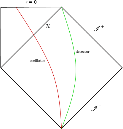
Figure 1: The Penrose-Carter diagram showing the oscillator on a free-fall trajectory in Painlevé-Gullstrand coordinates. The detector remains outside the black hole.

The relationship between Schwarzschild time $t_{s}$ and Painlevé-Gullstrand coordinates $(\tau,r)$ is:

$$dt_{s}=d\tau-\frac{\sqrt{2M/r}}{1-2M/r}dr.$$ (4)

In terms of the usual tortoise coordinate

$$r_{*}=r+2M\ln\left|\frac{r}{2M}-1\right|,$$ (5)

for $r>0$ we define the out-going null coordinates

$$u=t_{s}-r=\tau-\xi(r),$$ (6)

with

$$\xi(r)=r+2\sqrt{2Mr}+4M\ln\left(\sqrt{\frac{r}{2M}}-1\right),$$ (7)

and similarly, the in-going null coordinate for $r>0$,

$$v=t_{s}+r_{s}=\tau+\eta(r),$$ (8)

with

$$\eta(r)=r-2\sqrt{2Mr}+4M\ln\left(\sqrt{\frac{r}{2M}}+1\right).$$ (9)

We couple the oscillator to a massless scalar field $\Phi$ satisfying the Klein-Gordon equation,

$$\Box\Phi=0.$$ (10)

In P-G coordinates in 1+1 dimensions this is

$$(1-f)^{-1}\left[\frac{\partial}{\partial t}-(1-f)\frac{\partial}{\partial r}\right]\left[(1-f)\frac{\partial}{\partial t}+(1-f^{2})\frac{\partial}{\partial r}\right]=0$$ (11)

where $f=\sqrt{2M/r}$. In the right hand wedge the outgoing field can be expanded in terms of out-going modes $e^{\pm iku}$

$$\phi_{\mathrm{out}}=\sum_{k\geq 0}e_{k}\left\{b^{(0)}_{k}e^{-ik(t-\xi(r))}+b^{(0)\dagger}_{k}e^{ik(t-\xi(r)}\right\}$$ (12)

with the usual Klein-Gordon normalisation in a box of length $L$, $e_{k}=\sqrt{\frac{2\pi}{kL}}.$ Similarly we can express the field in terms of in-going modes $e^{\pm ikv}$ in the wedge $r>0$ as

$$\phi_{\mathrm{in}}=\sum_{k\geq 0}e_{k}\left\{b^{(0)}_{-k}e^{-ik(t+\eta(r))}+b^{(0)\dagger}_{-k}e^{ik(t+\eta(r))}\right\}.$$ (13)

In general, the full solution to the Klein-Gordon equation will be a linear combination of the ingoing and outgoing modes:

$$\Phi=\phi_{\mathrm{in}}+\phi_{\mathrm{out}}.$$ (14)

We define the vacuum state $|0\rangle$ by

$$b^{(0)}_{k}|0\rangle=0\quad\text{and}\quad b^{(0)}_{-k}|0\rangle=0.$$ (15)

We shall need the Fourier transforms of these modes as evaluated along the worldline of the infalling oscillator. We define

$$e^{ik(\tau-\xi(\tau))}=\left\{\begin{array}[]{l l}\displaystyle{\int_{-\infty}^{\infty}}\alpha_{k}(k^{\prime})e^{-ik^{\prime}\tau}\ dk^{\prime}&\quad\tau<-\tau_{s}\\ 0&\quad\tau>-\tau_{s}\\ \end{array}\right.$$ (16)

and

$$e^{ik(\tau+\eta(\tau))}=\left\{\begin{array}[]{l l}\displaystyle{\int_{-\infty}^{\infty}}\beta_{k}(k^{\prime})e^{-ik^{\prime}\tau}\ dk^{\prime}&\quad\tau<-\tau_{s}\\ 0&\quad\tau>-\tau_{s}.\\ \end{array}\right.$$ (17)

Approximate expressions for the Fourier components $\alpha_{k}(k^{\prime})$ and $\beta_{k}(k^{\prime})$ are obtained in appendix 1. We find

$$\alpha_{k}(k^{\prime}) =\frac{2M}{\pi}ke^{-2\pi Mk}e^{-iM(22k+4k^{\prime})/3}(4M)^{4iMk}(3k+k^{\prime})^{4iMk-1}\Gamma(-4iMk)$$ (18)

$$\beta_{k}(k^{\prime}) =2\sqrt{\frac{2M}{\pi|k|}}e^{i\pi/4}\exp\left\{iMk\left[-\frac{10}{3}+4\ln 2\right]+ik^{\prime}\tau_{s}-\frac{2iM}{k}(k+2k^{\prime})^{2}\right\}.$$ (19)

If $3k+k^{\prime}$ is real, then the branch in the imaginary power is defined by $3k+k^{\prime}=e^{-i\pi}|3k+k^{\prime}|$ for $3k+k^{\prime}<0.$

3 The Quantum Langevin Equation

We now derive the equation of motion for the oscillator. We take a quantum harmonic oscillator of mass $m$ and natural frequency $\omega$ confined to a free-fall worldline in $r>0$ with proper time $\tau$. We couple this to a massless scalar field $\Phi$ with a scalar-electrodynamic form for the interaction. Our Hamiltonian is therefore

$$\begin{split}\mathscr{H}=\omega a^{\dagger}a+&\sum_{k>0}\omega_{k}b^{\dagger}_{k}b_{k}+\sum_{k>0}\omega_{k}b^{\dagger}_{-k}b_{-k}\\ &ig\sqrt{\frac{\omega}{2m}}\sum_{k>0}e_{k}(a^{\dagger}-a)(b_{k}e^{ik\xi}+b^{\dagger}_{k}e^{-ik\xi}+b_{-k}e^{-i\omega_{k}\eta}+b^{\dagger}_{-k}e^{ik\eta})\end{split}$$ (20)

where $a^{\dagger}$ is the creation operator for the quantum oscillator, $\omega_{k}=|k|$, and $g$ is a coupling constant.

We do not make the rotating wave approximation at this point [13] to remove the products that pair creation operators of the field and oscillator (and similarly pairings of annihilation operators) both because keeping them here makes the calculation slightly easier and for comparison with the Unruh radiation in Scully et al. [20] later. We shall impose the rotating wave approximation appropriately below.

We now use Heisenberg’s equation of motion to determine the evolution of the oscillator and the scalar field. From

$$\frac{da}{d\tau}=-i[a,\mathscr{H}],$$ (21)

and putting $\lambda=g\sqrt{\omega/2m}$ for brevity, we obtain the equation of motion for the oscillator

$$\frac{da}{d\tau}=-i\omega a+\lambda\sum_{k}e_{k}(b_{k}e^{ik\xi}+b^{\dagger}_{k}e^{-ik\xi}+b_{-k}e^{-i\omega_{k}\eta}+b^{\dagger}_{-k}e^{ik\eta}).$$ (22)

Similarly, for the scalar field:

$$\frac{db_{j}}{d\tau}=-i[b_{j},\mathscr{H}],$$ (23)

from which we obtain

$$\frac{db_{k}}{d\tau}=-i\omega_{k}b_{k}+\lambda e_{k}(a^{\dagger}-a)e^{-ik\xi}\ \ \mathrm{and}\ \ \frac{db_{-k}}{d\tau}=-i\omega_{k}b_{-k}+\lambda e_{k}(a^{\dagger}-a)e^{ik\eta}.$$ (24)

We can solve (24) to obtain expressions for the scalar field operators:

$$b_{k}(\tau)=e^{-ik\tau}b_{k}^{(0)}+\lambda e^{-ik\tau}e_{k}\int_{-\infty}^{\tau}(a^{\dagger}-a)e^{ik(\tau^{\prime}-\xi(\tau^{\prime}))}\ d\tau^{\prime}$$ (25)

and

$$b_{-k}(\tau)=e^{-ik\tau}b_{-k}^{(0)}+\lambda e^{-ik\tau}e_{k}\int_{-\infty}^{\tau}(a^{\dagger}-a)e^{ik(\tau^{\prime}+\eta(\tau^{\prime}))}\ d\tau^{\prime}.$$ (26)

We assume that the interaction is switched on at some distant time $\tau>-\infty$ in the past when $\lambda\rightarrow 0$ and $b_{k}=b_{k}^{(0)}.$

We now go on to use (25) and (26) to derive an expression for the position operator for our oscillator. Direct substitution into (22) gives:

$$\begin{split}\frac{da}{d\tau}=&-i\omega a+\mathcal{G}_{a}+\lambda^{2}\sum_{k}e_{k}^{2}\bigg{\{}\\ &e^{-ik(\tau-\xi)}\int_{-\infty}^{\tau}(a^{\dagger}-a)e^{ik(\tau^{\prime}-\xi^{\prime})}\ d\tau^{\prime}-e^{ik(\tau-\xi)}\int_{-\infty}^{\tau}(a^{\dagger}-a)e^{-ik(\tau^{\prime}-\xi^{\prime})}\ d\tau^{\prime}\\ &+e^{-ik(\tau+\eta)}\int_{-\infty}^{\tau}(a^{\dagger}-a)e^{ik(\tau^{\prime}+\eta^{\prime})}\ d\tau^{\prime}-e^{ik(\tau+\eta)}\int_{-\infty}^{\tau}(a^{\dagger}-a)e^{-ik(\tau^{\prime}+\eta^{\prime})}\ d\tau^{\prime}\bigg{\}}\end{split}$$ (27)

with the function

$$\mathcal{G}_{a}(\tau)=\lambda\sum_{k}e_{k}\{b_{k}^{(0)}e^{-ik(\tau-\xi)}+b^{(0)\dagger}_{k}e^{ik(\tau-\xi)}+b_{-k}^{(0)}e^{-ik(\tau+\eta)}+b^{(0)\dagger}_{-k}e^{ik(\tau+\eta)}\}.$$ (28)

We now remove high frequency behaviour by setting

$$a(\tau)=e^{-i\omega\tau}A(\tau).$$ (29)

Using this and the Fourier transforms of (16) and (17) in (27) gives:

$$\begin{split}\frac{dA}{d\tau}=&\mathcal{G}_{A}+\lambda^{2}\sum_{k}e_{k}^{2}e^{i\omega\tau}\bigg{\{}\\ &\int_{-\infty}^{\infty}\alpha^{*}(k^{\prime\prime})e^{ik^{\prime\prime}\tau}\ dk^{\prime\prime}\int_{-\infty}^{\infty}\alpha_{k}(k^{\prime})\ dk^{\prime}\int_{-\infty}^{\tau}\left(e^{i(\omega-k^{\prime})\tau^{\prime}}A^{\dagger}-e^{-i(\omega+k^{\prime})\tau^{\prime}}A\right)\ d\tau^{\prime}\\ &-\int_{-\infty}^{\infty}\alpha(k^{\prime})e^{-ik^{\prime}\tau}\ dk^{\prime}\int_{-\infty}^{\infty}\alpha_{k}^{*}(k^{\prime\prime})\ dk^{\prime\prime}\int_{-\infty}^{\tau}\left(e^{i(\omega+k^{\prime\prime})\tau^{\prime}}A^{\dagger}-e^{-i(\omega-k^{\prime\prime})\tau^{\prime}}A\right)\ d\tau^{\prime}\\ &+\int_{-\infty}^{\infty}\beta^{*}(k^{\prime\prime})e^{ik^{\prime\prime}\tau}\ dk^{\prime\prime}\int_{-\infty}^{\infty}\beta_{k}(k^{\prime})\ dk^{\prime}\int_{-\infty}^{\tau}\left(e^{i(\omega-k^{\prime})\tau^{\prime}}A^{\dagger}-e^{-i(\omega+k^{\prime})\tau^{\prime}}A\right)\ d\tau^{\prime}\\ &-\int_{-\infty}^{\infty}\beta(k^{\prime})e^{-ik^{\prime}\tau}\ dk^{\prime}\int_{-\infty}^{\infty}\beta_{k}^{*}(k^{\prime\prime})\ dk^{\prime\prime}\int_{-\infty}^{\tau}\left(e^{i(\omega+k^{\prime\prime})\tau^{\prime}}A^{\dagger}-e^{-i(\omega-k^{\prime\prime})\tau^{\prime}}A\right)\ d\tau^{\prime}\bigg{\}}.\end{split}$$ (30)

The rotating wave approximation now amounts to neglecting the $A^{\dagger}$ terms since these behave like $e^{2\omega\tau}$. We could subsequently include these terms in an iterative solution, which would amount to taking into account the higher energy levels of the oscillator in the line profile, but this is not crucial for our discussion. (In effect we are treating the oscillator as a two-level atom.)

Next we perform the $\tau^{\prime}$ integrations using integration by parts:

$$\int_{-\infty}^{\tau}e^{-i(\omega+k^{\prime})\tau^{\prime}}A(\tau^{\prime})d\tau^{\prime}=\left[\frac{iA(\tau^{\prime})e^{-i(\omega+k^{\prime})\tau^{\prime}}}{\omega+k^{\prime}}\right]_{-\infty}^{\tau}-i\int_{-\infty}^{\tau}\frac{dA}{d\tau^{\prime}}\frac{e^{-i(\omega+k^{\prime})\tau^{\prime}}}{\omega+k^{\prime}}\ d\tau^{\prime}$$ (31)

We can neglect the final (integral) term in (31) because, from (30), it contributes a correction of order $\lambda^{2}$ to $\mathcal{G}_{A}$ and of order $\lambda^{4}$ to $dA/d\tau$. This method is equivalent to solving equation (30) via a Laplace transform as in Louisell [13]. (We demonstrate this equivalence in appendix 5.) The contribution from $\tau^{\prime}\rightarrow-\infty$ vanishes under our assumption that the interaction is switched off at early times. We are left with

$$\begin{split}\frac{dA}{d\tau}&=\mathcal{G}_{A}+i\lambda^{2}A(\tau)\sum_{k}e_{k}^{2}\bigg{\{}\\ &-\int_{-\infty}^{\infty}\alpha^{*}(k^{\prime\prime})e^{ik^{\prime\prime}\tau}dk^{\prime\prime}\int_{-\infty}^{\infty}\frac{\alpha_{k}(k^{\prime})e^{-ik^{\prime}\tau}dk^{\prime}}{\omega+k^{\prime}}+\int_{-\infty}^{\infty}\alpha(k^{\prime})e^{-ik^{\prime}\tau}dk^{\prime}\int_{-\infty}^{\infty}\frac{\alpha_{k}^{*}(k^{\prime\prime})e^{ik^{\prime\prime}\tau}dk^{\prime\prime}}{\omega-k^{\prime\prime}}\\ &-\int_{-\infty}^{\infty}\beta^{*}(k^{\prime\prime})e^{ik^{\prime\prime}\tau}dk^{\prime\prime}\int_{-\infty}^{\infty}\frac{\beta_{k}(k^{\prime})e^{-ik^{\prime}\tau}dk^{\prime}}{\omega+k^{\prime}}+\int_{-\infty}^{\infty}\beta(k^{\prime})e^{-ik^{\prime}\tau}dk^{\prime}\int_{-\infty}^{\infty}\frac{\beta_{k}^{*}(k^{\prime\prime})e^{ik^{\prime\prime}\tau}dk^{\prime\prime}}{\omega-k^{\prime\prime}}\bigg{\}}.\end{split}$$ (32)

This expression can be simplified by interchanging $k^{\prime}$ and $k^{\prime\prime}$ in the second integrals on each of the last two lines of equation (32) and using $\alpha_{k}(k^{\prime})=\alpha_{-k}^{*}(-k^{\prime})$ with a similar relation for $\beta_{k}(k^{\prime})$ to combine the integrals into a sum over $k$, $-\infty<k<\infty$. Finally, writing the sum over $k$ as an integral (i.e. letting $L\rightarrow\infty$) we get

$$\begin{split}\frac{dA}{d\tau}&=\mathcal{G}_{A}\\ &-i\lambda^{2}A(\tau)\int_{-\infty}^{\infty}\frac{dk}{k}\int_{-\infty}^{\infty}dk^{\prime}\int_{-\infty}^{\infty}dk^{\prime\prime}\left[\alpha_{k}^{*}(k^{\prime\prime})\alpha_{k}(k^{\prime})+\beta^{*}_{k}(k^{\prime\prime})\beta_{k}(k^{\prime})\right]\frac{e^{i(k^{\prime\prime}-k^{\prime})\tau}dk^{\prime}}{\omega+k^{\prime}}\end{split}$$ (33)

Defining ${\mathcal{G}_{A}}=e^{i\omega\tau}\mathcal{G}_{a}$, we write the quantum Langevin equation for the oscillator as

$$\frac{dA}{d\tau}=-\left(\frac{\gamma}{2}+i\Delta\omega\right)A(\tau)+\mathcal{G}_{A},$$ (34)

with the friction constant $\gamma$ and the Lamb shift $\Delta\omega$ implicitly given by (33).

We show in appendix 3 that

$$\gamma=\frac{\pi g^{2}}{m}.$$ (35)

The evaluation of the Lamb shift is more subtle and will be pursued elsewhere. Here we simply incorporate it into the definition of $\omega$.

Solving (34) we get

$$A(\tau)=e^{-\gamma\tau/2}\int_{-\infty}^{\tau}e^{\gamma\tau^{\prime}/2}\mathcal{G}_{A}(\tau^{\prime})\ d\tau^{\prime}$$ (36)

where we have ignored the initial value of $A$ since this gives rise to a transient signal far from the black hole and is consequently of no interest here.

Thus,

$$\begin{split}A(\tau)&=\\ &\lambda e^{-\gamma\tau/2}\sum_{k}e_{k}\left\{b_{k}^{(0)}\int_{-\infty}^{\tau}e^{i(\omega-i\gamma/2)\tau^{\prime}}e^{-ik(\tau^{\prime}-\xi(\tau^{\prime}))}d\tau^{\prime}+b^{(0)\dagger}_{k}\int_{-\infty}^{\tau}e^{i(\omega-i\gamma/2)\tau^{\prime}}e^{ik(\tau^{\prime}-\xi(\tau^{\prime}))}\ d\tau^{\prime}\right.\\ &\left.+b_{-k}^{(0)}\int_{-\infty}^{\tau}e^{i(\omega-i\gamma/2)\tau^{\prime}}e^{-ik(\tau^{\prime}+\eta(\tau^{\prime}))}d\tau^{\prime}+b^{(0)\dagger}_{-k}\int_{-\infty}^{\tau}e^{i(\omega-i\gamma/2)\tau^{\prime}}e^{ik(\tau^{\prime}+\eta(\tau^{\prime}))}\ d\tau^{\prime}\right\}.\end{split}$$ (37)

Using the Fourier transforms (16) and (17) gives:

$$\begin{split}A(\tau)&=\lambda e^{-\gamma\tau/2}\sum_{k}e_{k}\bigg{\{}\\ &b_{k}^{(0)}\int_{-\infty}^{\infty}\int_{-\infty}^{\tau}e^{i(\omega+k^{\prime}-i\gamma/2)\tau^{\prime}}\alpha^{*}(k^{\prime})d\tau^{\prime}dk^{\prime}+b^{(0)\dagger}_{k}\int_{-\infty}^{\infty}\int_{-\infty}^{\tau}e^{i(\omega-k^{\prime}-i\gamma/2)\tau^{\prime}}\alpha(k^{\prime})d\tau^{\prime}dk^{\prime}\\ &+b_{-k}^{(0)}\int_{-\infty}^{\infty}\int_{-\infty}^{\tau}e^{i(\omega+k^{\prime}-i\gamma/2)\tau^{\prime}}\beta^{*}(k^{\prime})d\tau^{\prime}dk^{\prime}+\left.b^{(0)\dagger}_{-k}\int_{-\infty}^{\infty}\int_{-\infty}^{\tau}e^{i(\omega-k^{\prime}-i\gamma/2)\tau^{\prime}}\beta(k^{\prime})d\tau^{\prime}dk^{\prime}\right\}.\end{split}$$ (38)

We define the oscillator susceptibility

$$\chi(k^{\prime})=\frac{1}{\omega+k^{\prime}-i\gamma/2}.$$ (39)

Performing the $\tau^{\prime}$ integrations we obtain

$$\begin{split}A(\tau)&=\\ &-i\lambda e^{i\omega\tau}\sum_{k}e_{k}\left\{b_{k}^{(0)}\int_{-\infty}^{\infty}e^{ik^{\prime}\tau}\alpha^{*}(k^{\prime})\chi(k^{\prime})dk^{\prime}+b^{(0)\dagger}_{k}\int_{-\infty}^{\infty}e^{-ik^{\prime}\tau}\alpha_{k}(k^{\prime})\chi(-k^{\prime})dk^{\prime}\right.\\ &\left.+b_{-k}^{(0)}\int_{-\infty}^{\infty}e^{ik^{\prime}\tau}\beta_{k}^{*}(k^{\prime})\chi(k^{\prime})dk^{\prime}+b^{(0)\dagger}_{-k}\int_{-\infty}^{\infty}e^{-ik^{\prime}\tau}\beta_{k}(k^{\prime})\chi(-k^{\prime})dk^{\prime}\right\}.\end{split}$$ (40)

In principle, this would allow us to determine how the oscillator comes into equilibrium with its local environment at any distance from the black hole. However, we know the $k^{\prime}$-dependence of $\alpha_{k}(k^{\prime})$ and $\beta_{k}(k^{\prime})$ only on the assumption that $\tau<\sim\tau_{s}$.

We now have everything we require to determine the position operator of the oscillator

$$q=\frac{1}{\sqrt{2\omega m}}(a^{\dagger}+a)$$ (41)

near the black hole. Using $A(\tau)=e^{i\omega\tau}a(\tau)$, and writing

$$\Delta\chi(k^{\prime})=\chi^{*}(k^{\prime})-\chi(-k^{\prime}),$$ (42)

the position operator of the harmonic oscillator, ignoring transients, becomes

$$\begin{split}q(\tau)=\frac{i\lambda}{\sqrt{2m\omega}}&\sum_{k}e_{k}\bigg{\{}\\ &b_{k}^{(0)}\int_{-\infty}^{\infty}e^{ik^{\prime}\tau}\alpha^{*}(k^{\prime})\Delta\chi(-k^{\prime})dk^{\prime}+b^{(0)\dagger}_{k}\int_{-\infty}^{\infty}e^{-ik^{\prime}\tau}\alpha_{k}(k^{\prime})\Delta\chi(k^{\prime})dk^{\prime}\\ +&\left.b_{-k}^{(0)}\int_{-\infty}^{\infty}e^{ik^{\prime}\tau}\beta^{*}(k^{\prime})\Delta\chi(-k^{\prime})dk^{\prime}+b^{(0)\dagger}_{-k}\int_{-\infty}^{\infty}e^{-ik^{\prime}\tau}\beta_{k}(k^{\prime})\Delta\chi(k^{\prime})dk^{\prime}\right\}.\end{split}$$ (43)

4 The Solution to the Field Equation

We now wish to determine the solution to the scalar field equation in the presence of the oscillator. In section 2 we determined that the scalar field $\Phi$ can be decomposed into a linear sum of in-going and outgoing modes:

$$\Phi=\sum_{k}e_{k}\left\{b_{k}e^{ik\xi}+b^{\dagger}_{k}e^{-ik\xi}+b_{-k}e^{-ik\eta}+b^{\dagger}_{-k}e^{ik\eta}\right\}.$$ (44)

In section 3 we determined expression for $b_{k}$ and $b_{-k}$; these are given in (25) and (26). Thus substituting into (44) we find that the field can be written as

$$\Phi=\Phi_{h}+\Phi_{p},$$ (45)

where the homogeneous part

$$\Phi_{h}=\sum_{k}e_{k}\left\{b_{k}^{(0)}e^{-ik(\tau-\xi)}+b_{k}^{\dagger(0)}e^{ik(\tau-\xi)}+b_{-k}^{(0)}e^{-ik(\tau+\eta)}+b_{-k}^{\dagger(0)}e^{-ik(\tau+\eta)}\right\},$$ (46)

and the particular integral is

$$\begin{split}\Phi_{p}=&\lambda\sum_{k}e_{k}^{2}\Big{\{}\\ &e^{-ik(\tau-\xi(\tau))}\int_{-\infty}^{\tau}(a^{\dagger}-a)e^{ik(\tau^{\prime}-\xi(\tau^{\prime}))}\ d\tau^{\prime}-e^{ik(\tau-\xi(\tau))}\int_{-\infty}^{\tau}(a^{\dagger}-a)e^{-ik(\tau^{\prime}-\xi(\tau^{\prime}))}\ d\tau^{\prime}\\ &e^{-ik(\tau+\eta(\tau))}\int_{-\infty}^{\tau}(a^{\dagger}-a)e^{ik(\tau^{\prime}+\eta(\tau^{\prime}))}\ d\tau^{\prime}-e^{ik(\tau+\eta(\tau))}\int_{-\infty}^{\tau}(a^{\dagger}-a)e^{-ik(\tau^{\prime}+\eta(\tau^{\prime}))}\ d\tau^{\prime}\Big{\}}.\end{split}$$ (47)

Using the relation between the annihilation and creation operators and the momentum, $p$,

$$p=m\frac{dq}{d\tau}=i\sqrt{\frac{m\omega}{2}}(a^{\dagger}-a),$$ (48)

we get

$$\begin{split}\Phi_{p}=-ig&\sum_{k}e_{k}^{2}\left\{\int_{-\infty}^{\tau}\frac{dq}{d\tau^{\prime}}\left(e^{ik(\tau^{\prime}-\tau)-ik(\xi(\tau^{\prime})-\xi(\tau))}-e^{-ik(\tau^{\prime}-\tau)+ik(\xi(\tau^{\prime})-\xi(\tau))}\right)\ d\tau^{\prime}\right.\\ &+\int_{-\infty}^{\tau}\frac{dq}{d\tau^{\prime}}\left.\left(e^{ik(\tau^{\prime}-\tau)+ik(\eta(\tau^{\prime})-\eta(\tau))}-e^{-ik(\tau^{\prime}-\tau)-ik(\eta(\tau^{\prime})-\eta(\tau))}\right)\ d\tau^{\prime}\right\}.\end{split}$$ (49)

Combining the exponentials and converting $\sum_{k}\rightarrow\int dk$ gives

$$\begin{split}\Phi_{p}=2g&\left[\int_{0}^{\infty}\int_{-\infty}^{\tau}\frac{1}{k}\frac{dq}{d\tau^{\prime}}\sin[k(\tau^{\prime}-\tau)-k(\xi(\tau^{\prime})-\xi(\tau)]\ dt\ dk\right.\\ &\left.+\int_{-\infty}^{0}\int_{-\infty}^{\tau}\frac{1}{k}\frac{dq}{d\tau^{\prime}}\sin[k(\tau^{\prime}-\tau)-k(\eta(\tau^{\prime})+\eta(\tau)]\ dt\ dk\right].\end{split}$$ (50)

We now set

$$I_{1}=\int_{0}^{\infty}\int_{-\infty}^{\tau}\frac{1}{k}\frac{dq}{d\tau^{\prime}}\sin[k(\tau^{\prime}-\tau)-k(\xi(\tau^{\prime})-\xi(\tau))]\ d\tau^{\prime}dk,$$ (51)

and

$$I_{2}=\int_{-\infty}^{0}\int_{-\infty}^{\tau}\frac{1}{k}\frac{dq}{d\tau^{\prime}}\sin[k(\tau^{\prime}-\tau)+k(\eta(\tau^{\prime})+\eta(\tau))]\ \tau^{\prime}dk.$$ (52)

Evaluating the $k$ integral in $I_{1}$ first, we see that this is just the retarded Green’s function in two dimensions [18], and so:

$$\mathscr{G}_{\mathrm{ret}}(\tau,\xi,\tau^{\prime},\xi^{\prime})=\left\{\begin{array}[]{cc}\pi&|\xi-\xi^{\prime}|<\tau-\tau^{\prime},\ \tau>\tau^{\prime}\\ 0&\mathrm{otherwise}\end{array}\right.$$ (53)

which means that

$$I_{1}=q(\tau_{\mathrm{ret}})$$ (54)

where $\tau_{\rm ret}$ is given by

$$\tau_{\rm ret}-\xi(\tau_{\rm ret})=\tau^{\prime}-\xi^{\prime}.$$ (55)

Evaluating $I_{2}$ we identify the $k$ integral in $I_{2}$ as being the advanced Green’s function, and if we let $k\rightarrow-k$

$$\mathscr{G}_{\mathrm{adv}}=\lim_{\epsilon\rightarrow 0}\left\{\frac{1}{2\pi}\int_{0}^{\infty}\int_{-\infty}^{\infty}\frac{e^{ik(\eta-\eta^{\prime})-ik^{0}(\tau-\tau^{\prime})}}{(k^{0}-i\epsilon)^{2}-k^{2}}\ dk^{0}dk.\right\}$$ (56)

Examining the $k^{0}$ integral we see that the simple poles are located in the upper-half of the complex plane. However we still require $\tau>\tau^{\prime}$ so we would form a semi-circular in the lower half of the complex plane which does not therefore enclose the poles. So this integral gives no contribution. Thus we have obtained the solution to the scalar field equation

$$\Phi(\tau,r)=\Phi_{h}+2\pi gq(\tau_{\mathrm{ret}}).$$ (57)

5 The Energy Flux at the Detector

We now look at the response of a detector at a large distance from the black hole. This operationalises the meaning of radiation from the infalling oscillator. For the accelerated detector in the Rindler wedge in [18] we calculated the noise power on the world line of a distant inertial detector, which is directly related to the probability of excitation of the detector. Here we shall look at the closely related, but more familiar, energy flux at the detector.

We shall demonstrate first that the energy flux at the detector has a blackbody form modulated by the impedance of the infalling body. This enables us to explain the difference between the Rindler case and a black hole. We also show that the oscillator emits a negative energy flux into the hole. We then use the explicit form for the impedance function of a harmonic oscillator to derive an explicit form for the energy flux from the infalling oscillator.

Let the P-G coordinates of the oscillator be $(\tau,\xi(\tau))$ and let the coordinates of the detector be $(t^{\prime},\xi^{\prime}(t^{\prime}))$. For $\xi^{\prime}>\xi$

$$\tau_{\rm ret}-\xi(\tau_{\rm ret})=t^{\prime}-\xi^{\prime},$$ (58)

and for $\xi^{\prime}<\xi$

$$\tau_{\rm ret}+\eta(\tau_{\rm ret})=t^{\prime}+\eta^{\prime}.$$ (59)

In P-G coordinates an orthonormal dyad in the rest frame of the detector is

$${\bf e}^{0}=(1,0),\quad{\bf e}^{1}=(x^{\prime},1).$$ (60)

The energy-momentum flux at the detector is

$$F=T^{\hat{1}}_{\hat{0}}=-T_{\hat{0}\hat{1}}=-\langle{\bf e}^{\mu}_{0}{\bf e}^{\nu}_{1}T_{\mu\nu}\rangle=-x^{\prime}T_{r^{\prime}r^{\prime}}+T_{t^{\prime}r^{\prime}},$$ (61)

where the components of $T_{\mu^{\prime}\nu^{\prime}}$ are obtained as usual from

$$T_{\mu^{\prime}\nu^{\prime}}=\frac{\partial\Phi}{\partial x^{\prime\mu}}\frac{\partial\Phi^{\dagger}}{\partial x^{\prime\nu}}-\frac{1}{2}g_{\mu^{\prime}\nu^{\prime}}\left(\frac{\partial\Phi}{\partial x^{\prime\lambda}}\right)^{2}.$$ (62)

Using (57), the expectation value of the energy momentum flux is obtained from

$$\begin{split}\left\langle\frac{\partial\Phi^{\dagger}}{\partial x^{\prime\mu}}\frac{\partial\Phi}{\partial x^{\prime\nu}}\right\rangle=&\left\langle\frac{\partial\Phi_{h}^{\dagger}}{\partial x^{\prime\mu}}\frac{\partial\Phi_{h}}{\partial x^{\prime\nu}}\right\rangle\\ &+2\pi g\left\langle\frac{\partial\Phi_{h}^{\dagger}}{\partial x^{\prime\mu}}\dot{q}(\tau_{ret})\frac{\partial\tau_{ret}}{\partial x^{\prime\nu}}+\dot{q^{\dagger}}(\tau_{ret})\frac{\partial\tau_{ret}}{\partial x^{\prime\mu}}\frac{\partial\Phi_{h}}{\partial x^{\prime\nu}}\right\rangle\\ &+4\pi g^{2}\left\langle\dot{q^{\dagger}}(\tau_{ret})\frac{\partial\tau_{ret}}{\partial x^{\prime\mu}}\dot{q}(\tau_{ret})\frac{\partial\tau_{ret}}{\partial x^{\prime\nu}}\right\rangle.\end{split}$$ (63)

The first term on the right of equation (63) involves only the unperturbed field and represents the flux present in the absence of the oscillator. The Hawking radiation is obtained by the standard calculation (e.g. [11]) that relates the incoming modes on $\mathscr{I}^{-}$ at $r\rightarrow-\infty$ that do not fall into the horizon (defining the in-vacuum) to the outgoing modes on $\mathscr{I}^{+}$ at $r\rightarrow+\infty$, defining the out-vacuum. In the Painlevé-Gullstrand manifold here (figure 1) there is only one vacuum state and no mixing of modes in the absence of the infalling oscillator. This term is therefore just the zero point flux and will have no influence on the detector. We can confirm this by an explicit calculation.

The normally ordered expression for the unperturbed $\langle:T_{\mu^{\prime}\nu^{\prime}}:\rangle$ based on the Painlevé-Gullstrand modes gives zero contribution. The covariant form can be calculated from the conformal factor, $e^{2\rho}=(1-f^{2})$, in the usual way for a 1+1 dimensional metric [7] [5]

$$\langle T_{uu}\rangle\propto\frac{\partial^{2}\rho}{\partial u^{2}}-\left(\frac{\partial\rho}{\partial u}\right)^{2}$$ (64)

with similar expressions for $\langle T_{vv}\rangle$. We obtain (up to a numerical factor)

$$\langle T_{uu}\rangle=\langle T_{vv}\rangle=\frac{M}{2r^{3}}-\frac{3M^{2}}{4r^{4}}$$ (65)

and

$$\langle T_{uv}\rangle=\frac{\partial^{2}\rho}{\partial u\partial v}=-\frac{M}{2r^{3}}\left(1-\frac{2M}{r}\right).$$ (66)

which vanish at infinity (exactly as in the Boulware vacuum). Thus there is no Hawking flux. (The flux on the horizon is formally non-zero, but this is non-physical since the coordinates do not satisfy the regularity conditions there [4].) Of course, the situation would be different if we were to take into account the collapse phase in the formation of the black hole, when this term would yield the usual Hawking effect.

The term on the second line of (63) represents the interference between the outgoing emission from the oscillator and the vacuum excitations of the detector. This is the flux we would get from first order perturbation theory treating the scalar field as an external potential. The final term in (63) represents the direct contribution to the flux arising from the oscillator.

We can tidy up equation (63) using the fact that the time dependence in $\Phi$ comes through $\tau_{\rm ret}$, since $\Phi_{h}(t^{\prime}-\xi^{\prime})=\Phi_{h}(\tau_{\rm ret}-\xi(\tau_{\rm ret}))$ and $q=q(\tau_{\rm ret})$. Thus the derivatives in $T_{\mu\nu}$ contribute factors of:

$$\frac{\partial\Phi}{\partial r^{\prime}}\frac{\partial\Phi^{\dagger}}{\partial r^{\prime}} \rightarrow \langle\dot{\Phi}\dot{\Phi}^{\dagger}\rangle\left(\frac{\partial\tau}{\partial\xi^{\prime}}\right)^{2}\left(\frac{\partial\xi^{\prime}}{\partial r^{\prime}}\right)^{2}$$

$$\frac{\partial\Phi}{\partial r^{\prime}}\frac{\partial\Phi^{\dagger}}{\partial t^{\prime}} \rightarrow \langle\dot{\Phi}\dot{\Phi}^{\dagger}\rangle\left(\frac{\partial\tau}{\partial\xi^{\prime}}\right)\left(\frac{\partial\xi^{\prime}}{\partial r^{\prime}}\right)\left(\frac{\partial\tau}{\partial t^{\prime}}\right)$$

$$\frac{\partial\Phi}{\partial t^{\prime}}\frac{\partial\Phi^{\dagger}}{\partial t^{\prime}} \rightarrow \langle\dot{\Phi}\dot{\Phi}^{\dagger}\rangle\left(\frac{\partial\tau}{\partial t^{\prime}}\right)^{2}$$

where $\dot{\Phi}=d\Phi/d\tau_{\rm ret}.$ Now, $q(\tau_{\rm ret})$ contributes a factor $\exp(\mp ik^{\prime}\tau_{\rm ret})$ to $\Phi$ and $\Phi_{h}=\phi_{\rm out}$ contributes a factor $\exp[\pm ik^{\prime}(t^{\prime}-\xi^{\prime})]=\exp[\pm ik^{\prime}(\tau_{\rm ret}-\xi(\tau_{\rm ret}))]$. Thus $\langle\dot{\Phi}\dot{\Phi}^{\dagger}\rangle=k^{\prime}k^{\prime\prime}\langle\Phi\Phi^{\dagger}\rangle$. Writing $f=\sqrt{2M/r}$, $f^{\prime}=\sqrt{2M/r^{\prime}}$ as above (for $r>0$, $r^{\prime}>0$), from the definitions (55) we find

$$\frac{\partial\tau}{\partial\xi^{\prime}}=-\frac{\partial\tau}{\partial t^{\prime}}=-(1-f)\quad\text{and}\quad\frac{\partial\xi^{\prime}}{\partial r^{\prime}}=\frac{1}{1-f^{\prime}}.\quad$$ (67)

Putting this together we find that

$$F=\frac{(1-f)^{2}}{(1-f^{\prime})^{2}}(\langle\mathcal{J}\rangle_{\mathrm{dir}}+\langle\mathcal{J}\rangle_{\mathrm{int}})$$ (68)

where

$$\begin{split}&\langle\mathcal{J}\rangle_{\mathrm{dir}}=4\pi g^{2}\langle\dot{q}^{\dagger}\dot{q}\rangle\\ =&\gamma^{2}\sum_{k}e_{k}^{2}\int_{-\infty}^{\infty}\int_{-\infty}^{\infty}k^{\prime}k^{\prime\prime}e^{i(k^{\prime\prime}-k^{\prime})\tau_{\mathrm{ret}}}\Delta\chi(k^{\prime})\Delta\chi^{*}(k^{\prime\prime})[\alpha_{k}(k^{\prime})\alpha_{k}^{*}(k^{\prime\prime})+\beta_{k}(k^{\prime})\beta^{*}(k^{\prime\prime})]\ dk^{\prime}dk^{\prime\prime}.\end{split}$$ (69)

with $\gamma=\pi g^{2}/m$ (equation (35)) and $\Delta\chi$ is given by (42). The interference term for the detector at $\xi^{\prime}>\xi$ is given by

$$\begin{split}\langle\mathcal{J}\rangle_{\mathrm{int}}=&2\pi g\langle\dot{q}^{\dagger}\dot{\phi_{\rm out}}+\dot{q}\dot{\phi}_{\rm out}^{\dagger}\rangle\\ =&-\gamma\sum_{k}e_{k}^{2}\int_{-\infty}^{\infty}\int_{-\infty}^{\infty}k^{\prime}k^{\prime\prime}e^{i(k^{\prime\prime}-k^{\prime})\tau_{\mathrm{ret}}}\alpha_{k}(k^{\prime})\alpha_{k}^{*}(k^{\prime\prime})[i\Delta\chi^{*}(k^{\prime\prime})+i\Delta\chi(k^{\prime})]\ dk^{\prime}\ dk^{\prime\prime}.\end{split}$$ (70)

We can write the redshift in terms of proper time along the world line of the oscillator. We have

$$\bar{\tau}\equiv\tau+\tau_{s}=\tau_{s}\left(1-\frac{1}{f^{3}}\right)=\frac{\tau_{s}}{f^{3}}(f-1)(f^{2}+f+1).$$ (71)

So the redshift factor in the flux is $\propto\bar{\tau}^{2},$ the proper time measured to the horizon and so for the oscillator close to the horizon and the detector at infinity ($x\sim 1$, $x^{\prime}\sim 0$),

$$F=\left(\frac{\bar{\tau}}{9\tau_{s}}\right)^{2}(\langle\mathcal{J}\rangle_{\mathrm{int}}+\langle\mathcal{J}\rangle_{\mathrm{dir}}).$$ (72)

We now proceed to compare the direct flux and the interference term. In appendix 2 we look at the stationary phase approximation to the $k^{\prime}$ and $k^{\prime\prime}$ integrals in equations (69) and (70). The result is that the impedance terms, $\Delta\chi$, are evaluated at the stationary points. This allows us to write $\langle\mathcal{J}\rangle_{\mathrm{dir}}$ as

$$\begin{split}\langle\mathcal{J}\rangle_{\mathrm{dir}}=&\gamma^{2}\int_{0}^{\infty}\frac{dk}{k}\int_{-\infty}^{\infty}dk^{\prime\prime}\int_{-\infty}^{\infty}\ dk^{\prime}\Big{\{}k^{\prime}k^{\prime\prime}e^{i(k^{\prime\prime}-k^{\prime})\tau_{\rm ret}}\\ &\times\left[\alpha_{k}^{*}(k^{\prime\prime})\alpha_{k}(k^{\prime})|\Delta\chi(k_{\alpha})|^{2}+\beta_{k}^{*}(k^{\prime\prime})\beta_{k}(k^{\prime})|\Delta\chi(k_{\beta})|^{2}\right]\Big{\}}.\end{split}$$ (73)

where we have inserted the stationary points

$$k^{\prime}(k)=k_{\alpha}=\frac{(-3k\tau_{\rm ret})}{\bar{\tau}}\ \ \mathrm{and}\ \ k^{\prime}(k)=k_{\beta}=-2k$$ (74)

given in appendix 2. We now compare this with the interference term. Again, we use the stationary phase approximation to justify writing $\langle\mathcal{J}\rangle_{\mathrm{int}}$ (equation (70)) as

$$\langle\mathcal{J}\rangle_{\mathrm{int}}=-2\gamma\int_{0}^{\infty}\frac{dk}{k}\int_{-\infty}^{\infty}\int_{-\infty}^{\infty}e^{i(k^{\prime\prime}-k^{\prime})\tau_{\mathrm{ret}}}\alpha_{k}(k^{\prime})\alpha_{k}^{*}(k^{\prime\prime})[i\Delta\chi^{*}(k_{\alpha})+i\Delta\chi(k_{\alpha})].$$ (75)

We now use the fluctuation-dissipation theorem (appendix 4) to write this as

$$\langle\mathcal{J}\rangle_{\mathrm{int}}=-2\gamma^{2}\int_{0}^{\infty}\frac{dk}{k}\int_{-\infty}^{\infty}\int_{-\infty}^{\infty}e^{i(k^{\prime\prime}-k^{\prime})\tau_{\mathrm{ret}}}\alpha_{k}(k^{\prime})\alpha_{k}^{*}(k^{\prime\prime})|\Delta\chi(k_{\alpha})|^{2}.$$ (76)

Comparing with equation (73) we see that the total flux (up to the redshift factor) is

$$\begin{split}\langle\mathcal{J}\rangle_{\mathrm{dir}}+\langle\mathcal{J}\rangle_{\mathrm{int}}=&\gamma^{2}\int_{0}^{\infty}\frac{dk}{k}\int_{-\infty}^{\infty}dk^{\prime\prime}\int_{-\infty}^{\infty}\ dk^{\prime}\Big{\{}k^{\prime}k^{\prime\prime}e^{i(k^{\prime\prime}-k^{\prime})\tau_{\rm ret}}\\ &\left[-\alpha_{k}^{*}(k^{\prime\prime})\alpha_{k}(k^{\prime})|\Delta\chi(k_{\alpha})|^{2}+\beta_{k}^{*}(k^{\prime\prime})\beta_{k}(k^{\prime})\right]|\Delta\chi(k_{\beta})|^{2}\Big{\}}\\ \equiv&-\mathcal{F}_{\alpha}+\mathcal{F}_{\beta}.\end{split}$$ (77)

Note that if it were the case that $\alpha_{k}(k^{\prime})=\beta_{k}(k^{\prime})$, then $k_{\alpha}=k_{\beta}$ and this expression vanishes. This accords with our result for the case of a constantly accelerated oscillator in flat spacetime.

In the case that $\alpha_{k}(k^{\prime})\neq\beta_{k}(k^{\prime})$, the flux at the detector does not vanish. If we place the detector closer to the hole than the oscillator, the interference term now involves the ingoing modes. Thus it makes a contribution $-2\mathcal{F}_{\beta}$ to the flux which therefore becomes $-F$. Thus, if the energy radiated to infinity by the infalling oscillator is positive, the energy radiated into the hole is negative.

Given our particular forms for $\alpha_{k}(k^{\prime})$ and $\beta_{k}(k^{\prime})$ corresponding to a freely-falling oscillator we proceed to show that the flux has a blackbody spectrum (modified by the oscillator impedance) as the oscillator approaches the black hole.

We can write the fluxes in equation (77) as

$$\mathcal{F}_{\alpha}=\gamma^{2}\int_{0}^{\infty}\frac{dk}{k}I_{\alpha}(k)I^{*}_{\alpha}(k)$$ (78)

where

$$I_{\alpha}(k)=\int_{-\infty}^{\infty}k^{\prime}\alpha_{k}(k^{\prime})e^{-ik^{\prime}\tau}\Delta\chi(k^{\prime})dk^{\prime}$$ (79)

with corresponding definitions for $\mathcal{F}_{\beta}$ and $I_{\beta}(k)$. The susceptibility factor is peaked around $k^{\prime}=\pm\omega$. The stationary phase approximation to the integral for $k>0$ will turn out to require $k^{\prime}<0.$ Thus we can make the replacement $\Delta\chi(k^{\prime})=\chi^{*}(k^{\prime})-\chi(-k^{\prime})\approx\chi^{*}(k^{\prime}).$ This corresponds to keeping the energy conserving terms $a^{\dagger}b+ab^{\dagger}$ in the Hamiltonian. We shall find that the remaining terms that give rise to the Unruh effect (coming from $a^{\dagger}b^{\dagger}+ab$ in $\mathscr{H}$) give a contribution $\gamma/\omega$ smaller.

We now have

$$I_{\alpha}(k)=\frac{2Mk}{\pi}e^{2\pi Mk}e^{-2\pi iMk}e^{i(\pi/2-2\omega/\gamma)}(4M)^{4iMk}\Gamma(-4iMk)J_{1}$$ (80)

where

$$J_{1}=\int_{-\infty}^{\infty}dk^{\prime}e^{-ik^{\prime}\bar{\tau}}(3k^{\prime}+k)^{4iMk}f(k^{\prime})$$ (81)

with

$$f(k^{\prime})=k^{\prime}(3k+k^{\prime})^{-1}\Delta\chi(k^{\prime}).$$ (82)

Evaluating $J_{1}$ for large $Mk$ by stationary phase (appendix 2) gives

$$J_{1}\sim(2\pi)^{1/2}e^{-4iMk+3ik\tau-i\pi/4}(4Mk)^{4iMk-1/2}\bar{\tau}^{-4iMk}f\left(\frac{-3k\tau}{\bar{\tau}}\right).$$ (83)

The contribution to the flux from $I_{\alpha}(k)I^{*}_{\alpha}(k)$ is therefore

$$\begin{split}-\mathcal{F}_{\alpha}=&-9\gamma^{2}\left(\frac{\tau}{\bar{\tau}}\right)^{2}\int_{0}^{\infty}kB(-8\pi Mk)\frac{dk}{(\omega+k^{\prime}(k))^{2}+\gamma^{2}/4}\\ =&-\gamma^{2}\int_{0}^{-\infty}k^{\prime}B\left(2\pi\bar{\tau}k^{\prime}\right)\frac{dk^{\prime}}{(\omega+k^{\prime})^{2}+\gamma^{2}/4},\end{split}$$ (84)

where we have substituted $k^{\prime}(k)=-3k\tau/\bar{\tau}$ and taken the limit $\tau\rightarrow\tau_{s},$ and where the black-body function $B(x)$ is:

$$B(x)=\frac{1}{e^{x}-1}=-B(-x)-1.$$ (85)

Finally, we can extend the integration to the full range with an error of order $\gamma/\omega$ since

$$\begin{split}\int_{0}^{\infty}\frac{dk}{(\omega+k)^{2}+\gamma^{2}/4}=&\int_{\omega}^{\infty}\frac{dx}{x^{2}+\gamma^{2}/4}=\frac{1}{\gamma}\int_{\omega/\gamma}^{\infty}\frac{dy}{y^{2}+1}\\ \sim&\frac{1}{\gamma}\left(\frac{\gamma}{\omega}\right).\end{split}$$

This contribution to the flux is therefore

$$-\mathcal{F}_{\alpha}=-\gamma^{2}\int_{-\infty}^{\infty}k^{\prime}B\left(2\pi\bar{\tau}k^{\prime}\right)\frac{dk^{\prime}}{(\omega+k^{\prime})^{2}+\gamma^{2}/4}$$ (86)

where the integration is now over the full range of $k^{\prime}$.

Two comments are required here. The appearance of the blackbody factor arises from the Fourier analysis of the time dependence of the oscillator trajectory. It may seem strange that approximating the Fourier integral in (16) and its inverse transform in (79) introduces a blackbody factor. This arises through our treatment of the gamma functions which for consistency should strictly be evaluated in the asymptotic (large $Mk$) limit. Doing this would lead to the Wien tail of the blackbody emission. However, we shall stick with precedent (dating back to Hawking’s original paper) and retain the full blackbody form.

The second comment is the equally apparently strange way in which taking the Fourier transform followed by its inverse leads us merely to a form for $k^{\prime}(k)$ in the oscillator susceptibility which is not contributing to the phase. In fact, including the phase of the susceptibility in the stationary phase approximation makes no difference to the result to the lowest order in $\gamma/\omega$. An alternative approach is to note that the susceptibility is peaked around $k^{\prime}=\omega$ and to expand the integrand about this point. To the accuracy of our approximation this leads to the same final result.

To calculate the contribution from the ingoing ($\beta$) modes we start from (78) with

$$I_{\beta}=4\left(\frac{2M}{\pi k}\right)^{1/2}e^{iMk(-10/3+4\ln 2)+i\pi/4}\int_{-\infty}^{\infty}k^{\prime}\Delta\chi(k^{\prime})e^{i[-k^{\prime}\bar{\tau}+(2M/k)(k+2k^{\prime})^{2}]}dk^{\prime}.$$ (87)

We evaluate this again by stationary phase. We let

$$\phi(k^{\prime})=-k^{\prime}\bar{\tau}+\frac{2M}{k}(2k^{\prime}+k)^{2}.$$ (88)

The stationary point is

$$k^{\prime}(k)=-\frac{k}{2}\left(\frac{\bar{\tau}}{8M}+1\right)$$ (89)

from which we obtain

$$\int_{-\infty}^{\infty}k^{\prime}\Delta\chi(k^{\prime})e^{i[-k^{\prime}\bar{\tau}+(2M/k)(k+2k^{\prime})^{2}]}dk^{\prime}\sim-\frac{k^{3/2}}{2}\left(\frac{2\pi}{M}\right)^{1/2}\left(\frac{\bar{\tau}}{8M}+1\right)e^{i[\bar{\tau}k/2-\bar{\tau}^{2}k/(32M)]}\Delta\chi(k^{\prime}(k)).$$ (90)

The dominant term in $\Delta\chi$ comes from $\chi(+k^{\prime})$. Thus, to lowest order in $\gamma$, as $\bar{\tau}\rightarrow 0$

$$\begin{split}\mathcal{F}_{\beta}=\gamma^{2}\int_{0}^{\infty}\frac{dk}{k}I_{\beta}I^{*}_{\beta}&\sim\gamma^{2}\int_{0}^{\infty}\frac{k}{16}|\chi(k^{\prime}(k))|^{2}dk\\ &\sim-\gamma^{2}\int_{-\infty}^{\infty}\frac{k^{\prime}dk^{\prime}}{(\omega+k^{\prime})^{2}+\gamma^{2}/4}\\ \end{split}$$ (91)

Now use the relation $B(x)=-B(-x)-1$ to write (84) as

$$-\mathcal{F}_{\alpha}=-\gamma^{2}\int_{-\infty}^{\infty}k^{\prime}[-B(2\pi\bar{\tau}k^{\prime})-1]\frac{dk}{(\omega+k^{\prime}(k))^{2}+\gamma^{2}/4}.$$ (92)

This gives a positive frequency blackbody term plus the zero point energy that cancels the contribution from $I_{\beta}$. The total flux is therefore

$$\langle\mathcal{J}\rangle_{\mathrm{dir}}+\langle\mathcal{J}\rangle_{\mathrm{int}}=\gamma^{2}\int_{-\infty}^{\infty}k^{\prime}[B(2\pi\bar{\tau}k^{\prime})]\frac{dk}{(\omega+k^{\prime}(k))^{2}+\gamma^{2}/4}.$$ (93)

As promised, the result is a blackbody spectrum modulated by the oscillator susceptibility.

We now proceed to evaluate the remaining integral over wave number in (93). This has the form of a smoothly varying factor multiplied by the susceptibility which (for an under-damped oscillator) is peaked around $k^{\prime}=-\omega$. (We have $k^{\prime}(k)=-3k\tau/\bar{\tau}<0$ since $k>0$, which justifies the inclusion of only the terms in $k^{\prime}+\omega$ in (79)). We have

$$\int_{0}^{-\infty}\frac{k^{\prime}dk^{\prime}}{(\omega+k^{\prime})^{2}+\gamma^{2}/4}=\int_{-\infty}^{\infty}\frac{dx}{x^{2}+\gamma^{2}/4}+\mathcal{O}(\gamma/\omega)=\frac{2\pi}{\gamma}$$ (94)

giving

$$F\sim 2\pi\left(\frac{\bar{\tau}}{9\tau_{s}}\right)^{2}\gamma\omega B(2\pi\omega(-\bar{\tau}))$$ (95)

for $|\bar{\tau}|>\omega^{-1}$ and $|\bar{\tau}|<\sim M$, where we have re-instated the redshift factor (equation (72)).The blackbody factor peaks at $\bar{\tau}\omega\sim 1$ and the flux at the peak is of order $\gamma\omega/(M^{2}\omega^{2})$ or $(t_{d}/t_{in})(\lambda/R_{s})$ where $t_{d}\sim 1/\gamma$ is the decay (or equilibration) time, $t_{in}\sim M$ is the infall time, $\lambda=1/\omega$ is the wavelength of the oscillator and $R_{s}$ is the radius of the black hole.

For $\bar{\tau}<\omega^{-1}$ the oscillator susceptibility is no longer peaked, but we can evaluate the flux as follows. For $\omega\bar{\tau}\rightarrow 0$ we have

$$|\chi(k^{\prime})|^{2}=[(\omega+k^{\prime}(k))^{2}+\gamma^{2}/4]^{-1}\sim\bar{\tau}^{2}(9k^{2}\tau^{2}+\bar{\tau}^{2}\gamma^{2}/4)^{-1}.$$ (96)

The contribution to the total flux is

$$\begin{split}F_{0}&=9\gamma^{2}\left(\frac{\tau}{\bar{\tau}}\right)^{2}\int_{0}^{\infty}kB(8\pi Mk)\frac{\bar{\tau}^{2}dk}{9k^{2}\tau^{2}+\bar{\tau}^{2}\gamma^{2}/4}\\ &\sim\gamma^{2}\int_{0}^{\infty}B(8\pi Mk)\frac{d(MK)}{Mk}.\end{split}$$ (97)

as $\bar{\tau}\rightarrow 0$ and $\tau\rightarrow\tau_{s}$. The divergence at the lower limit can be dealt with by insisting that we are considering the case $Mk>1$ or by a more accurate treatment of the stationary phase, which brings in an extra factor of $4Mk(16M^{2}k^{2}+1)^{-1}$ (see appendix 3). In either case the contribution is proportional to $\gamma^{2}$ which is $\gamma/\omega$ smaller than $F$. We can therefore ignore this contribution.

We can estimate the total energy, $E$, emitted by integrating (95) over time, $t^{\prime}$, at the detector. Taking into account the redshift factors from (68), and $dt^{\prime}=\frac{dt^{\prime}}{d\tau}d\tau=\frac{\tau_{s}}{\bar{\tau}}d\bar{\tau}$, we have

$$\begin{split}E=&\pi\gamma\omega\int_{-\infty}^{\omega^{-1}}B(-2\pi\omega\bar{\tau})\left(\frac{\bar{\tau}}{\tau_{s}}\right)d\bar{\tau}\\ =&\frac{3\gamma}{16\pi M\omega}\int_{2\pi}^{\infty}xB(x)dx.\end{split}$$ (98)

We can write this in terms of the infall time $t_{\rm in}$, the decay time of the oscillator $t_{\rm d}$ and the wavelength $\lambda=1/\omega$ as

$$E\sim\omega\frac{\gamma M}{\omega^{2}M^{2}}\sim\omega\left(\frac{t_{\rm in}}{t_{\rm d}}\right)\left(\frac{\lambda}{R_{s}}\right)^{2}$$ (99)

for $\lambda<\sim R_{s}$. Note how the time-dependence of the infall in (98) spreads the expectation value of the energy from the oscillator at frequency $\omega$ (or more precisely, the renormalised frequency) into a blackbody spectrum.

6 Discussion

We can summarise our conclusions as follows. The infalling oscillator emits positive energy to infinity and negative energy into the black hole. This arises from the difference between the outgoing and ingoing modes (brought about by the cross-term in the metric, which provides the time asymmetry). The flux comes from a distance $>1/\omega$ from the horizon. This suggests that as long as the ingoing modes are close to Painlevé-Gullstrand modes the oscillator radiates even if the true horizon does not form [1].

The dominant effect comes from the energy conserving term in the Hamiltonian. (The atom is de-excited and emits a (scalar) photon. This is possible because the usual balance between excitation and de-excitation that results in the stability of the ground state is disturbed by the difference between ingoing and outgoing modes. Thus the ground state is no longer stable moment by moment. The Unruh terms in the Hamiltonian in this case yield a blackbody flux to infinity (and a negative flux into the hole), which is a factor $\gamma/\omega$ smaller than the dominant terms. In this model, the Unruh effect would dominate by neglecting the back-reaction of the field on the oscillator. Indeed, if we replace $\chi(k^{\prime})$ in (70) by $\lim_{\gamma\rightarrow 0}\chi(k^{\prime})=i\pi\delta(k^{\prime}+\omega)$ and put $\nu=-2k/3$ (the minus sign allowing for the energy non-conserving term in $\mathscr{H}$) we obtain the expression for the energy flux equivalent to that in Scully et al.[20] (although in the Boulware vacuum of their choice, this would be cancelled by the contribution from the direct flux).

As a simple model we can imagine a shell of oscillators (or atoms) collapsing to form a black hole. They radiate a blackbody flux to infinity and a negative energy flux into the (putative) black hole. But the emission from the oscillators is not the Hawking radiation: the flux from the oscillators depends on the strength of the matter-field coupling, so is not independent of their material properties; it occurs on a collapse timescale, not the Hawking timescale; and furthermore the flux is independent of the mass of the black hole (although spectrum depends on $M$ and the total energy radiated depends on $M$ through the infall time). Nevertheless, the model may provide some useful hints.

In a self-consistent picture, the black hole is bathed in both incoming negative energy fluctuations and outflowing positive energy. The fluctuations in this radiation field will perturb the hole and cause it to radiate. Thus, in the fuller picture, the emission can be seen as a two-quantum process. Furthermore, the second quantum carries information about the first. In other words, it is conceivable that information is not lost in the process in much the same way that it is not lost in the ”burning paper” illustration. In other words, we need to consider the reaction of the hole not just to its own radiation, but to that from the infalling matter (which, if nothing else, will be coupled to gravity). This may alter the argument from timescales [14].

One final speculation based on the model presented here. The Lamb shift is usually absorbed into the mass of the oscillator by renormalisation and therefore in effect neglected. In a Bohr atom $\omega\propto m$, the electron mass, so the energy radiated (which we found to be proportional to $\omega$) is the (renormalised) mass. This suggests we need to incorporate a theoretical account of the origin of mass into the theory if we are to understand the quantum mechanics of black holes.

Appendix 1: Fourier Transforms $\alpha_{k}(k^{\prime})$ and $\beta_{k}(k^{\prime})$ of the Modes

We have defined $\alpha_{k}(k^{\prime})$ as the Fourier transform of the out-going modes evaluated along the worldline of the oscillator,

$$\alpha_{k}(k^{\prime})=\frac{1}{2\pi}\int_{-\infty}^{-\tau_{s}}e^{ik(\tau-\xi(\tau))}e^{ik^{\prime}\tau}\ d\tau,$$ (100)

where $\tau=-\tau_{s}=-4M/3$ is the location of the event horizon. The worldline of the oscillator in free-fall is, in Painlevé-Gullstrand coordinates,

$$r_{s}(\tau)=\left(\frac{9M}{2}\right)^{\frac{1}{3}}(-\tau)^{2/3}.$$ (101)

with the function $\xi(r)$ defined as:

$$\xi(r)=r+2\sqrt{2Mr}+4M\ln\left(\sqrt{\frac{r}{2M}}-1\right).$$ (102)

When evaluated on the worldline of the oscillator this becomes:

$$\xi(\tau)=\left(\frac{9M}{2}\right)^{1/3}(-\tau)^{2/3}+(48M^{2})^{1/3}(-\tau)^{1/3}+4M\ln\left[\left(\frac{3}{4M}\right)^{1/3}(-\tau)^{1/3}-1\right]$$ (103)

The behaviour of the integral is dominated by the argument of the exponential at the endpoint of the range, namely near the horizon. We therefore expand $\xi(\tau)$ about the horizon with

$$\tau_{0}=-\tau_{s}-\epsilon$$ (104)

where $\epsilon>0$ is small compared to $\tau_{s}$. Note that this expansion means that we remain in the exterior region. Performing the expansion for each of the terms in (103) yields the asymptotic form

$$\xi(\epsilon)\approx 6M+2\epsilon+4M\ln(\epsilon)-4M\ln(4M),$$ (105)

and

$$\tau_{0}-\xi(\epsilon)\approx-\frac{22M}{3}-3\epsilon-4M\ln(\epsilon)+4M\ln(4M).$$ (106)

Using this expansion in (100) means that

$$\alpha_{k}(k^{\prime})=\frac{1}{2\pi}e^{-iM(22k+4k^{\prime})/3}(4M)^{4iMk}\int_{0}^{\infty}e^{-i(3k+k^{\prime})\epsilon}\epsilon^{-4iMk}\ d\epsilon.$$ (107)

The integral over $\epsilon$ may be converted into a Gamma function. To do this, we use the result from [2]:

$$\Gamma(z)=s^{z}\int_{0}^{\infty\ e^{i\delta}}e^{-st}t^{z-1}\ dt,$$ (108)

with $-(\pi/2+\delta)<\mathrm{arg}\ s<\pi/2-\delta$, $\Re(z)>0$. This result holds for $\mathrm{arg}\ s+\delta=\pm\pi/2$ provided $0<\Re(z)<1$. Applying this to our $\epsilon$-integral we obtain, after some algebra, that for $(3k+k^{\prime})>0$

$$\alpha_{k}(k^{\prime})=\frac{2M}{\pi}ke^{-2\pi Mk}e^{-iM(22k+4k^{\prime})/3}(4M)^{4iMk}(3k+k^{\prime})^{4iMk-1}\Gamma(-4iMk)$$ (109)

and for $(3k+k^{\prime})<0$

$$\alpha_{k}(k^{\prime})=-\frac{2M}{\pi}ke^{2\pi Mk}e^{-iM(22k+4k^{\prime})/3}(4M)^{4iMk}(-3k-k^{\prime})^{4iMk-1}\Gamma(-4iMk).$$ (110)

We now determine an approximate expression for the Fourier transform $\beta_{k}(k^{\prime})$ of the in-going modes along the worldline of the oscillator.

$$\begin{split}\beta_{k}(k^{\prime})=&\frac{1}{2\pi}\int_{-\infty}^{\tau_{s}}e^{ik(\tau+\eta(\tau))}e^{ik^{\prime}\tau}\ d\tau\\ =&\frac{1}{2\pi}\int_{-\infty}^{\tau_{s}}e^{ikM\phi(\tau)}\ d\tau\end{split}$$ (111)

with

$$\eta(r)=r-2\sqrt{2Mr}+4M\ln\left(\sqrt{\frac{r}{2M}}+1\right).$$ (112)

We are treating $Mk$ as a large parameter in the integrand. Since $\phi(\tau)$ does not have a stationary point in the range (or in $(-\infty,0)$), we expand about the end point on the horizon. (In fact, our result for the energy flux is independent of the point chosen to the accuracy of the approximation.) Define $t=-\tau/\tau_{s}=3\tau/4M$. Then, expanding $\phi(\tau)$ to second order gives

$$k\phi(t)=-\frac{10}{3}+4\ln 2-\frac{1}{3}(t-1)+\frac{1}{18}(t-1)^{2}+\frac{4}{3}k^{\prime}t.$$ (113)

In terms of $y=\sqrt{k\tau_{s}/24}(t-1)$, the integral for $\beta_{k}(k^{\prime})$ becomes

$$\beta_{k}(k^{\prime})\sim\frac{1}{\pi^{2}}\left(\frac{6\tau_{s}}{k}\right)^{1/2}\int_{-\infty}^{\infty}dy\exp\left\{\mp i\left[y+\sqrt{\frac{2M}{|k|}(k+2k^{\prime})}\right]^{2}+\frac{2M}{k}(k+2k^{\prime})^{2}\right\}$$ (114)

with the signs $\pm$ according as $k>0$ or $k<0$. We justify the extension of the range to $-\infty$ as follows. We are going to use this expression in the approximate evaluation of the energy flux by stationary phase about the stationary point $2k^{\prime}+k=-ik(t-1)/3$, with $k>0$, which gives a term $-4y^{2}$ in the exponential. Thus the integrand converges rapidly as $y\rightarrow+\infty$. We obtain

$$\beta_{k}(k^{\prime})=2\sqrt{\frac{2M}{\pi|k|}}e^{iMk(-10/3+4\ln(2))\pm i\pi/4+i\tau_{s}k^{\prime}-i\frac{2M}{k}(k+2k^{\prime})^{2}}.$$ (115)

Appendix 2: Evaluation of integrals by stationary phase

We want to evaluate integrals of the form

$$I(k)=\int_{-\infty}^{\infty}e^{-iu\bar{\tau}+4iMk\ln u}f(u)\frac{du}{u}$$ (116)

where $u=(3k+k^{\prime})$ and $\bar{\tau}=\tau+\tau_{s}<0$ and $f(u)$ is a smoothly varying function of $u$. We have

$$I(k)=\int_{-\infty}^{\infty}e^{i\phi(u)}f(u)du$$ (117)

where

$$\phi(u)=-u\bar{\tau}+(4Mk+i)\ln u.$$ (118)

The stationary point occurs at $u=u_{0}=\frac{-4Mk+i}{\bar{\tau}}$. We therefore have

$$\phi^{\prime\prime}(u_{0})=-\bar{\tau}^{2}/(4Mk+i).$$

Thus

$$\begin{split}I(k)&\sim e^{i\phi(u_{0})}f(u_{0})\int_{-\infty}^{\infty}\exp\left[\frac{i}{2}\phi^{\prime\prime}(u_{0})(u-u_{o})^{2}\right]du\\ &=e^{-i\pi/4}e^{i\phi(u_{0})}f(u_{0})\left[\frac{2\pi(4Mk+i)}{\bar{\tau}^{2}}\right]^{1/2}\\ &=(2\pi)^{1/2}e^{-i\pi/4}e^{(1-4iMk)}\left(4Mk+i\right)^{4iMk-1/2}f((4Mk+i)/\bar{\tau})\end{split}$$ (119)

and

$$\begin{split}I(k)I^{*}(k)&=2\pi e^{2}(4Mk+i)^{4iMk}(4Mk-i)^{-4iMk}(16M^{2}k^{2}+1)^{1/2}f\left(\frac{4Mk-i}{\bar{\tau}}\right)f\left(\frac{4Mk+i}{\bar{\tau}}\right)\\ &=2\pi e^{2}(16M^{2}k^{2}+1)^{1/2}\exp[{-8Mk\tan^{-1}(4Mk)^{-1}}]\left|f\left(\frac{4Mk-i}{\bar{\tau}}\right)\right|^{2}.\end{split}$$ (120)

In the large $Mk$ limit we have

$$I(k)\sim(2\pi)^{1/2}e^{-i\pi/4}e^{-4iMk}\left(4Mk\right)^{4iMk-1/2}f((4Mk)/\bar{\tau})$$ (121)

which is the form we would obtain directly from (116) and which we use in the body of the text.

Appendix 3 Evaluation of the decay rate, $\gamma$

Let $\Gamma=\gamma/2+i\Delta\omega$, then we have

$$\begin{split}\Gamma&=i\frac{\omega g^{2}}{2m}\int_{-\infty}^{\infty}\int_{-\infty}^{\infty}\int_{-\infty}^{\infty}\frac{dk}{k}\left[\alpha^{*}_{k}(k^{\prime\prime})\alpha_{k}(k^{\prime})+\beta_{k}(k^{\prime})\beta^{*}_{k}(k^{\prime\prime})\right]\frac{e^{i(k^{\prime\prime}-k^{\prime})\tau}}{\omega+k^{\prime}}dk^{\prime\prime}dk^{\prime}\\ &=\Gamma_{\alpha}+\Gamma_{\beta},\end{split}$$ (122)

where $\alpha_{k}(k^{\prime})$ and $\beta_{k}(k^{\prime})$ are given by (18) and (19). We are going to evaluate the $k^{\prime}$ and $k^{\prime\prime}$ integrals by stationary phase. It will turn out that the stationary point lies in the region $3k+k^{\prime}<0$ so we use the corresponding form for the $\alpha_{k}(k^{\prime})$. Then, from appendix 2, we have

$$I_{1}=\int_{-\infty}^{\infty}\alpha_{k}^{*}(k^{\prime\prime})e^{ik^{\prime\prime}\tau}dk^{\prime\prime}=-\frac{2eMk}{(i\pi\bar{\tau})^{1/2}}e^{2\pi Mk}\Gamma(4iMk)e^{i\psi}\left(\frac{4Mk-i}{\bar{\tau}}\right)^{-4iMk-1/2}$$ (123)

where $\psi=4iMk+22iMk/3-3ik\tau$.

Similarly

$$I_{2}=\int_{-\infty}^{\infty}\alpha_{k}(k^{\prime})e^{-ik^{\prime}\tau}\frac{dk^{\prime}}{\omega+k^{\prime}}=I_{1}^{*}\times(\omega)^{-1}\left(1-\frac{3k\tau}{\omega\bar{\tau}}+\frac{i}{\omega\bar{\tau}}\right)^{-1}$$ (124)

In the large $Mk$ limit we have

$$(4kM\pm i)^{\pm 4iMk}=(16M^{2}k^{2}+1)^{1/2}\exp\left[\pm 4Mk\tan^{-1}(\pm 1/4Mk)\right]\sim e^{-1}.$$ (125)

Finally we obtain

$$i\frac{\omega g^{2}}{2m}I_{1}I_{2}=\frac{i\lambda^{2}M}{\omega}\int_{-\infty}^{\infty}\frac{e^{4\pi Mk}}{\sinh(4\pi Mk)}(1+16M^{2}k^{2})^{-1/2}\left(1-\frac{3k\tau}{\omega\bar{\tau}}+\frac{i}{\omega\bar{\tau}}\right)^{-1}dk$$ (126)

To evaluate this we consider the large $Mk$ limit as $\tau\rightarrow\tau_{s}$. Provided the oscillator is more than a small fraction of $\tau_{s}$ outside he horizon, this implies that $\omega\bar{\tau}$ is large. (Large here means $>\ \mathcal{O}(1)$ since the integrand is exponentially decreasing as a function of $Mk$). Thus we can write

$$\frac{1}{1-\frac{3k\tau}{\omega\bar{\tau}}+\frac{i}{\omega\bar{\tau}}}=i\pi\delta\left(1-\frac{3k\tau}{\omega\bar{\tau}}\right)+{\rm PP}$$ (127)

where PP stands for the principal part of the integral. The delta function then restricts $k$ to $k=\omega\bar{\tau}/3\tau\sim-\omega\bar{\tau}/4M>0$ and the contribution to $\gamma/2$ from the outgoing modes is

$$\gamma/2=-\frac{\pi\lambda^{2}}{2\omega}B(-2\pi\omega\bar{\tau}\tau_{s}/\tau)=-\frac{\pi\lambda^{2}}{2\omega}[-1+B(2\pi\omega\bar{\tau})]\rightarrow\pi g^{2}/4m$$ (128)

for $\bar{\tau}$ of order $M$ in the large $Mk$ limit (i.e.for $\bar{\tau}\gg\omega^{-1}$).

We now have to consider the ingoing modes (the terms in $\beta_{k}(k^{\prime})$ in (19)). Note that the contribution to $\gamma$ comes from the zero point energy, so we expect the ingoing modes to make an equal contribution to $\gamma$. We want to evaluate

$$\Gamma_{\beta}=i\lambda^{2}\int_{-\infty}^{\infty}\int_{-\infty}^{\infty}\int_{-\infty}^{\infty}\frac{dk}{k}\beta_{k}(k^{\prime})\beta^{*}_{k}(k^{\prime\prime})\frac{e^{i(k^{\prime\prime}-k^{\prime})\tau}}{\omega+k^{\prime}}dk^{\prime\prime}dk^{\prime}.$$ (129)

To ensure convergence of the Fourier integrals we add a small imaginary part to $k^{\prime}$. Inserting the expressions for $\beta_{k}(k^{\prime})$ from (19) we find the condition for stationary phase is $k^{\prime}(k)=-(k/2)(1+\bar{\tau}/M)\rightarrow-k/2$ and the contribution to $\gamma/2$ is

$$\frac{\gamma}{2}=i\lambda^{2}\Re\left(\lim_{\epsilon\rightarrow 0}\left\{\int\frac{dk}{k}\frac{1}{(\omega-2k/3-i\epsilon)}\right\}\right)=\frac{\pi g^{2}}{4m}.$$ (130)

(We ignore the infrared divergence from the pole at $k=0$ since we are restricted to large $Mk$; in any case, it is an artefact of 1+1 dimensions.)

Thus, in the vicinity of the black hole, the equal contributions from $\Gamma_{\alpha}$ and $\Gamma_{\beta}$ sum to give

$$\frac{\gamma}{2}=\frac{\pi g^{2}}{2m}.$$ (131)

Appendix 4: The Fluctuation-Dissipation Theorem

First we determine an expression for $|\chi^{*}(k)-\chi(-k)|^{2}$ using the definition given in (39):

$$|\chi^{*}(k)-\chi(-k)|^{2}=\left|\frac{1}{\omega+k+i\gamma/2}-\frac{1}{\omega-k-i\gamma/2}\right|^{2}$$ (132)

We have that:

$$\Delta\chi(k)=\chi^{*}(k)-\chi(-k)=\frac{-2k-i\gamma}{(\omega+k+i\gamma/2)(\omega-k-i\gamma/2)}$$ (133)

Thus:

$$|\chi^{*}(k)-\chi(-k)|^{2}=\frac{4k^{2}+\gamma^{2}}{(\omega^{2}-k^{2})^{2}+\gamma^{2}(\omega^{2}+k^{2})/2+\gamma^{4}/4}$$ (134)

We also have

$$i\chi(k)+i\chi^{*}(k)=-\frac{\gamma}{2(\omega+k)^{2}+\gamma^{2}/2}$$ (135)

and hence

$$(i\chi(k)+i\chi^{*}(k))-(i\chi(-k)+i\chi^{*}(-k))=\frac{4\gamma\omega k}{(\omega_{c}^{2}-k^{2})^{2}+\gamma^{2}\omega k+\gamma^{4}/16}$$ (136)

The functions (134) and (136) are peaked around $k=\omega.$ Also $\gamma\ll\omega.$ Thus

$$|\chi^{*}(k)-\chi(-k)|^{2}\sim\frac{4\omega^{2}}{(\omega^{2}-k^{2})^{2}+\gamma^{2}\omega^{2}}$$ (137)

and

$$(i\chi(k)+i\chi^{*}(k))-(i\chi(-k)+i\chi^{*}(-k))\sim\frac{4\gamma\omega^{2}}{(\omega_{c}^{2}-k^{2})^{2}+\gamma^{2}\omega^{2}}$$ (138)

giving us the final result

$$i\Delta\chi(k)+i\Delta\chi^{*}(k)=\gamma|\Delta\chi(k)|^{2}$$ (139)

which is our fluctuation-dissipation theorem. Note that we use the theorem to establish the relationship between the direct and interference terms at the detector, but we use the exact expression for the impedances in evaluating the integrals over frequency.

Appendix 5: Derivation of the Langevin Equation

The integro-differential equation for the oscillator annihilation operator $A(t)$ derived from the Hamiltonian (20) with the rotating wave approximation is [13] (where $\kappa_{j}\rightarrow\lambda$ in our notation)

$$\frac{dA}{dt}=-\sum_{j}|\kappa_{j}|^{2}\int_{0}^{t}A(t^{\prime})e^{i(\omega_{j}-\omega)(t^{\prime}-t)}\ dt^{\prime}+G_{A}$$ (140)

where

$$G_{A}=-i\sum_{j}\kappa_{j}b_{j}(0)e^{-i\omega_{j}t}.$$ (141)

To ensure convergence of the Fourier transform we give $\omega_{j}$ a small imaginary part, $\omega_{j}\rightarrow\omega_{j}-i\epsilon$.

The Wigner-Weisskopff approach to solving this equation involves taking the Laplace transform of both sides, and then applying an approximation, which essentially allows the replacement of (140) by the Langevin equation

$$\frac{dA}{dt}=-\left(\frac{1}{2}\gamma+i\Delta\omega\right)A(t)+G_{A}(t),$$ (142)

where

$$\gamma=2\pi g(\omega)|\kappa(\omega)|^{2}\ \ \mathrm{and}\ \ \Delta\omega=-\int\frac{g(\omega_{j})|\kappa(\omega_{j})|^{2}\ d\omega_{j}}{\omega_{j}-\omega}.$$ (143)

This approach works because the Laplace transform leads to an equation for $\tilde{A}(s)$, the Laplace transform of $A(t)$. This method is not available to us since the Laplace transform of (140) does not yield an equation for $\tilde{A}(s)$. (We could expand $\tilde{A}$ as a power series in $s$ but it is then difficult to control the approximation.) We now show that the Langevin equation may be obtained using integration by parts. Returning to (140) we integrate by parts with respect to $t^{\prime}$ :

$$\int_{0}^{t}A(t^{\prime})e^{i(\omega_{j}-\omega)(t^{\prime}-t)}\ dt^{\prime}=\frac{A(t)}{i(\omega_{j}-\omega)}-\frac{A(0)e^{-i(\omega_{j}-\omega)t}}{i(\omega_{j}-\omega)}-\int_{0}^{t}\frac{dA}{dt^{\prime}}\frac{e^{i(\omega_{j}-\omega)(t^{\prime}-t)}}{i(\omega_{j}-\omega)}\ dt^{\prime}.$$ (144)

The integral in (144) is of order $g$ smaller than the other terms, so can be neglected. The term in $A(0)$ represents the initial conditions and can be neglected in the differential equation. Thus (140) now becomes:

$$\frac{dA}{dt}=iA(t)\sum_{j}\frac{|\kappa(\omega_{j})|^{2}e^{i(\omega_{j}-\omega)t}}{\omega_{j}-\omega}+G_{A}.$$ (145)

We now convert the sum over $j$ into an integral over $\omega_{j}$:

$$\sum_{j}|\kappa(\omega_{j})|^{2}\rightarrow\int_{0}^{\infty}g(\omega_{j})|\kappa(\omega_{j})|^{2}\ d\omega_{j},$$

and so, with $\omega_{j}\rightarrow\omega_{j}-i\epsilon$ then:

$$\frac{dA}{dt}=G_{A}+iA(t)\int_{0}^{\infty}\frac{|\kappa(\omega_{j})|^{2}g(\omega_{j})e^{i(\omega_{j}-\omega-i\epsilon)t}}{\omega_{j}-\omega-i\epsilon}\ d\omega_{j}$$ (146)

Using the Sokhotski-Plemelj theorem [16]

$$\begin{split}\lim_{s\rightarrow 0}\int_{0}^{\infty}\frac{|\kappa(\omega_{j})|^{2}g(\omega_{j})e^{i(\omega_{j}-\omega-is)t}}{\omega_{j}-\omega-is}\ d\omega_{j}=&\mathcal{P}\left(\int_{0}^{\infty}\frac{|\kappa(\omega_{j})|^{2}g(\omega_{j})e^{i(\omega_{j}-\omega)t}}{\omega_{j}-\omega}\ d\omega_{j}\right)\\ &+i\pi\int_{0}^{\infty}|\kappa(\omega_{j})|^{2}g(\omega_{j})e^{i(\omega_{j}-\omega)t}\delta(\omega_{j}-\omega)\ d\omega_{j}\end{split}$$ (147)

Thus, after integrating out the delta function:

$$\frac{dA}{dt}=G_{A}-(\pi|\kappa(\omega)|^{2}g(\omega)+i\Delta\omega)A(t)$$ (148)

which gives (142) with $\gamma$ and $\Delta\omega$ as defined in (143)