Triple descent and the Two Kinds of Overfitting:
Where & Why do they Appear?

Abstract

A recent line of research has highlighted the existence of a “double descent” phenomenon in deep learning, whereby increasing the number of training examples $N$ causes the generalization error of neural networks to peak when $N$ is of the same order as the number of parameters $P$. In earlier works, a similar phenomenon was shown to exist in simpler models such as linear regression, where the peak instead occurs when $N$ is equal to the input dimension $D$. Since both peaks coincide with the interpolation threshold, they are often conflated in the litterature. In this paper, we show that despite their apparent similarity, these two scenarios are inherently different. In fact, both peaks can co-exist when neural networks are applied to noisy regression tasks. The relative size of the peaks is then governed by the degree of nonlinearity of the activation function. Building on recent developments in the analysis of random feature models, we provide a theoretical ground for this sample-wise triple descent. As shown previously, the nonlinear peak at $N\!=\!P$ is a true divergence caused by the extreme sensitivity of the output function to both the noise corrupting the labels and the initialization of the random features (or the weights in neural networks). This peak survives in the absence of noise, but can be suppressed by regularization. In contrast, the linear peak at $N\!=\!D$ is solely due to overfitting the noise in the labels, and forms earlier during training. We show that this peak is implicitly regularized by the nonlinearity, which is why it only becomes salient at high noise and is weakly affected by explicit regularization. Throughout the paper, we compare analytical results obtained in the random feature model with the outcomes of numerical experiments involving deep neural networks.

Introduction

A few years ago, deep neural networks achieved breakthroughs in a variety of contexts [1, 2, 3, 4]. However, their remarkable generalization abilities have puzzled rigorous understanding [5, 6, 7]: classical learning theory predicts that generalization error should follow a U-shaped curve as the number of parameters $P$ increases, and a monotonous decrease as the number of training examples $N$ increases. Instead, recent developments show that deep neural networks, as well as other machine learning models, exhibit a starkly different behaviour. In the absence of regularization, increasing $P$ and $N$ respectively yields parameter-wise and sample-wise double descent curves [8, 9, 10, 11, 12, 13], whereby the generalization error first decreases, then peaks at the interpolation threshold (at which point training error vanishes), then decreases monotonically again. This peak was shown to be related to a sharp increase in the variance of the estimator [18, 9], and can be suppressed by regularization or ensembling procedures [9, 19, 20].

Although double descent has only recently gained interest in the context of deep learning, a seemingly similar phenomenon has been well-known for several decades for simpler models such as least squares regression [21, 22, 23, 14, 15], and has recently been studied in more detail in an attempt to shed light on the double descent curve observed in deep learning [24, 25, 26, 27]. However, in the context of linear models, the number of parameters $P$ is not a free parameter: it is necessarily equal to the input dimension $D$. The interpolation threshold occurs at $N\!=\!D$, and coincides with a peak in the test loss which we refer to as the linear peak. For neural networks with nonlinear activations, the interpolation threshold surprisingly becomes independent of $D$ and is instead observed when the number of training examples is of the same order as the total number of training parameters, i.e. $N\!\sim\!P$: we refer to the corresponding peak as the nonlinear peak.

Somewhere in between these two scenarios lies the case of neural networks with linear activations. They have $P\!>\!D$ parameters, but only $D$ of them are independent: the interpolation threshold occurs at $N\!=\!D$. However, their dynamical behaviour shares some similarities with that of deep nonlinear networks, and their analytical tractability has given them significant attention [28, 29, 6]. A natural question is the following: what would happen for a “quasi-linear” network, e.g. one that uses a sigmoidal activation function with a high saturation plateau? Would the overfitting peak be observed both at $N\!=\!D$ and $N\!=\!P$, or would it somehow lie in between?

In this work, we unveil the similarities and the differences between the linear and nonlinear peaks. In particular, we address the following questions:

• Are the linear and nonlinear peaks two different phenomena?

• If so, can both be observed simultaneously, and can we differentiate their sources?

• How are they affected by the activation function? Can they both be suppressed by regularizing or ensembling? Do they appear at the same time during training?

Contribution

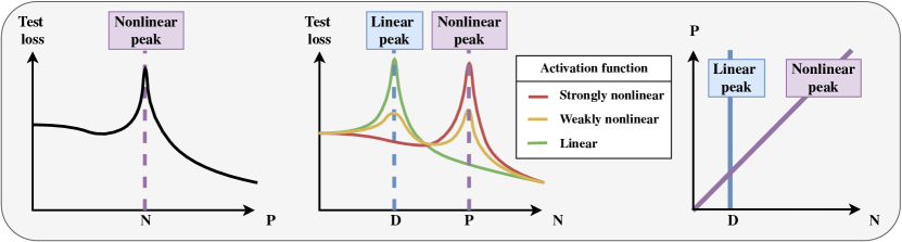
Figure 1: Left: The parameter-wise profile of the test loss exhibits double descent, with a peak at $P\!=\!N$. Middle: The sample-wise profile can, at high noise, exhibit a single peak at $N\!=\!P$, a single peak at $N\!=\!D$, or a combination of the two (triple descent) depending on the degree of nonlinearity of the activation function. Right: Color-coded location of the peaks in the $(P,N)$ phase space.

In modern neural networks, the double descent phenomenon is mostly studied by increasing the number of parameters $P$ (Fig. 2, left), and more rarely, by increasing the number of training examples $N$ (Fig. 2, middle) [13]. The analysis of linear models is instead performed by varying the ratio $P/N$. By studying the full $(P,N)$ phase space (Fig. 2, right), we disentangle the role of the linear and the nonlinear peaks in modern neural networks, and elucidate the role of the input dimension $D$.

In Sec.1, we demonstrate that the linear and nonlinear peaks are two different phenomena by showing that they can co-exist in the $(P,N)$ phase space in noisy regression tasks. This leads to a sample-wise triple descent, as sketched in Fig. 2. We consider both an analytically tractable model of random features [30] and a more realistic model of neural networks.

In Sec. 2, we provide a theoretical analysis of this phenomenon in the random feature model. We examine the eigenspectrum of random feature Gram matrices and show that whereas the nonlinear peak is caused by the presence of small eigenvalues [6], the small eigenvalues causing the linear peak gradually disappear when the activation function becomes nonlinear: the linear peak is implicitly regularized by the nonlinearity. Through a bias-variance decomposition of the test loss, we reveal that the linear peak is solely caused by overfitting the noise corrupting the labels, whereas the nonlinear peak is also caused by the variance due to the initialization of the random feature vectors (which plays the role of the initialization of the weights in neural networks).

Finally, in Sec. 3, we present the phenomenological differences which follow from the theoretical analysis. Increasing the degree of nonlinearity of the activation function weakens the linear peak and strengthens the nonlinear peak. We also find that the nonlinear peak can be suppressed by regularizing or ensembling, whereas the linear peak cannot since it is already implicitly regularized. Finally, we note that the nonlinear peak appears much later under gradient descent dynamics than the linear peak, since it is caused by small eigenmodes which are slow to learn.

Related work

Various sources of sample-wise non-monotonicity have been observed since the 1990s, from linear regression [14] to simple classification tasks [31, 32]. In the context of adversarial training, [33] shows that increasing $N$ can help or hurt generalization depending on the strength of the adversary. In the non-parametric setting of [34], an upper bound on the test loss is shown to exhibit multiple descent, with peaks at each $N=D^{i},i\in\mathbb{N}$.

Two concurrent papers also discuss the existence of a triple descent curve, albeit of different nature to ours. On one hand, [19] observes a sample-wise triple descent in a non-isotropic linear regression task. In their setup, the two peaks stem from the block structure of the covariance of the input data, which presents two eigenspaces of different variance; both peaks boil down to what we call “linear peaks”. [35] pushed this idea to the extreme by designing the covariance matrix in such a way to make an arbitrary number of linear peaks appear.

On the other hand, [36] presents a parameter-wise triple descent curve in a regression task using the Neural Tangent Kernel of a two-layer network. Here the two peaks stem from the block structure of the covariance of the random feature Gram matrix, which contains a block of linear size in input dimension (features of the second layer, i.e. the ones studied here), and a block of quadratic size (features of the first layer). In this case, both peaks are “nonlinear peaks”.

The triple descent curve presented here is of different nature: it stems from the general properties of nonlinear projections, rather than the particular structure chosen for the data [19] or regression kernel [36]. To the best of our knowledge, the disentanglement of linear and nonlinear peaks presented here is novel, and its importance is highlighted by the abundance of papers discussing both kinds of peaks.

On the analytical side, our work directly uses the results for high-dimensional random features models derived in [11, 37] (for the test loss), [38] (for the spectral analysis) and [20] (for the bias-variance decomposition).

Reproducibility

We release the code necessary to reproduce the data and figures in this paper publicly at https://github.com/sdascoli/triple-descent-paper.

1 Triple descent in the test loss phase space

We compute the ($P,N$) phase space of the test loss in noisy regression tasks to demonstrate the triple descent phenomenon. We start by introducing the two models which we will study throughout the paper: on the analytical side, the random feature model, and on the numerical side, a teacher-student task involving neural networks trained with gradient descent.

Dataset

For both models, the input data ${\bm{X}}\in\mathbb{R}^{N\times D}$ consists of $N$ vectors in $D$ dimensions whose elements are drawn i.i.d. from $\mathcal{N}(0,1)$. For each model, there is an associated label generator $f^{\star}$ corrupted by additive Gaussian noise: $y=f^{\star}({\bm{x}})+\epsilon$, where the noise variance is inversely related to the signal to noise ratio (SNR), $\epsilon\sim\mathcal{N}(0,1/\mathrm{SNR})$.

1.1 Random features regression (RF model)

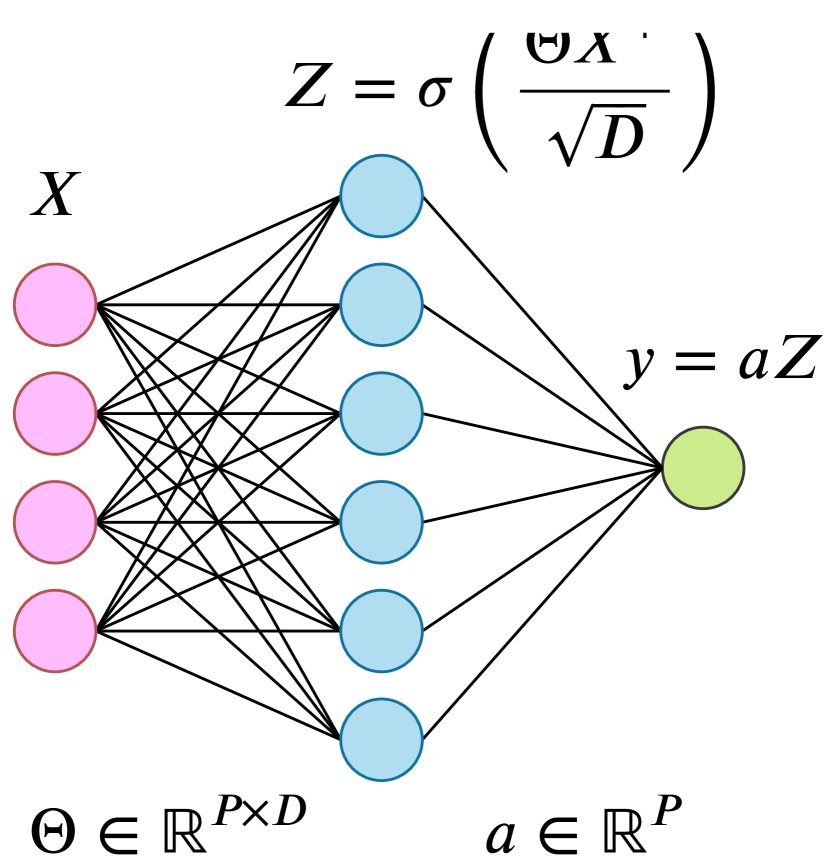
Figure 2: Illustration of an RF network.

Model

We consider the random features (RF) model introduced in [30]. It can be viewed as a two-layer neural network whose first layer is a fixed random matrix ${\bm{\Theta}}\in\mathbb{R}^{P\times D}$ containing the $P$ random feature vectors (see Fig. 2):

$$f({\bm{x}})=\sum_{i=1}^{P}{\bm{a}}_{i}\sigma\left(\frac{\langle{\bm{\Theta}}_{i},{\bm{x}}\rangle}{\sqrt{D}}\right).$$ (1)

$\sigma$ is a pointwise activation function, the choice of which will be of prime importance in the study. The ground truth is a linear model given by $f^{\star}({\bm{x}})=\langle{\bm{\beta}},{\bm{x}}\rangle/\sqrt{D}$. Elements of ${\bm{\Theta}}$ and ${\bm{\beta}}$ are drawn i.i.d from $\mathcal{N}(0,1)$.

Training

The second layer weights, i.e. the elements of ${\bm{a}}$, are calculated via ridge regression with a regularization parameter $\gamma$:

$$\bm{\hat{a}} =\underset{\bm{a}\in\mathbb{R}^{P}}{\arg\min}\left[\frac{1}{N}\left({\bm{y}}-{\bm{a}}\bf Z^{\top}\right)^{2}+\frac{P\gamma}{D}\|\bm{a}\|_{2}^{2}\right]=\frac{1}{N}{\bm{y}}^{\top}{\bm{Z}}\left({\bm{\Sigma}}+\frac{P\gamma}{D}\mathbb{I}_{P}\right)^{-1}$$ (2)

$${\bm{Z}}_{i}^{\mu} =\sigma\left(\frac{\langle{\bm{\Theta}}_{i},{\bm{X}}_{\mu}\rangle}{\sqrt{D}}\right)\in\mathbb{R}^{N\times P},\quad{\bm{\Sigma}}=\frac{1}{N}{\bm{Z}}^{\top}{\bm{Z}}\in\mathbb{R}^{P\times P}$$ (3)

1.2 Teacher-student regression with neural networks (NN model)

Model

We consider a teacher-student neural network (NN) framework where a student network learns to reproduce the labels of a teacher network. The teacher $f^{\star}$ is taken to be an untrained ReLU fully-connected network with 3 layers of weights and 100 nodes per layer. The student $f$ is a fully-connected network with 3 layers of weights and nonlinearity $\sigma$. Both are initialized with the default PyTorch initialization.

Training

We train the student with mean-square loss using full-batch gradient descent for 1000 epochs with a learning rate of 0.01 and momentum 0.9. We examine the effect of regularization by adding weight decay with parameter 0.05, and the effect of ensembling by averaging over 10 initialization seeds for the weights. All results are averaged over these 10 runs.

1.3 Test loss phase space

In both models, the key quantity of interest is the test loss, defined as the mean-square loss evaluated on fresh samples ${\bm{x}}\sim\mathcal{N}(0,1)$: $\mathcal{L}_{g}=\operatorname*{\mathbb{E}}_{{\bm{x}}}\left[\left(f({\bm{x}})-f^{\star}({\bm{x}})\right)^{2}\right].$

In the RF model, this quantity was first derived rigorously in [11], in the high-dimensional limit where $N,P,D$ are sent to infinity with their ratios finite. More recently, a different approach based on the Replica Method from Statistic Physics was proposed in [37]; we use this method to compute the analytical phase space. As for the NN model, which operates at finite size $D\!=\!196$, the test loss is computed over a test set of $10^{4}$ examples.

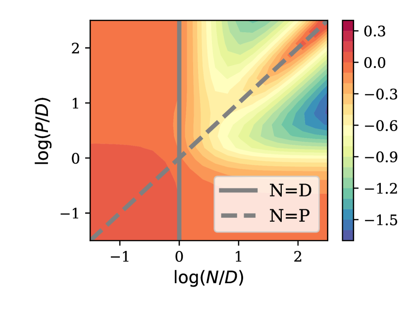
(a) RF, $SNR\!=\!2$

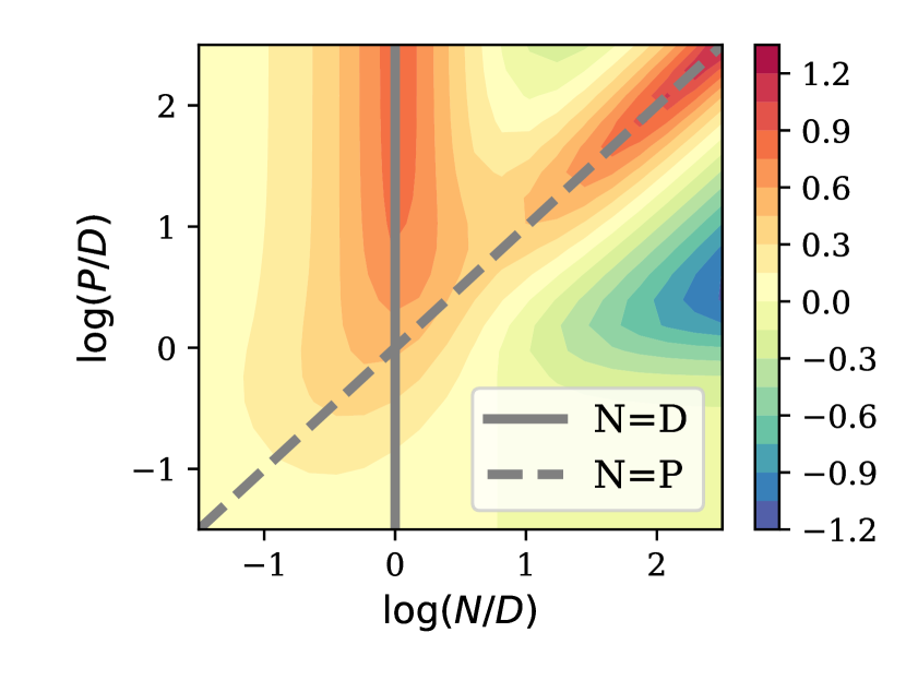
(b) RF, $SNR\!=\!0.2$

(c) NN, $SNR\!=\!0.2$

Figure 3: Logarithmic plot of the test loss in the $(P,N)$ phase space. (a): RF model with $\mathrm{SNR}=2$, $\gamma\!=\!10^{-1}$. (b): RF model with $\mathrm{SNR}=0.2$, $\gamma\!=\!10^{-1}$. The solid arrows emphasize the sample-wise profile, and the dashed lines emphasize the parameter-wise profile. (c): NN model. In all cases, $\sigma=\mathrm{Tanh}$. Analogous results for different activation functions and values of the SNR are shown in Sec. A of the SM.

In Fig.3, we plot the test loss as a function of two intensive ratios of interest: the number of parameters per dimension $P/D$ and the number of training examples per dimension $N/D$. In the left panel, at high SNR, we observe an overfitting line at $N\!=\!P$, yielding a parameter-wise and sample-wise double descent. However when the SNR becomes smaller than unity (middle panel), the sample-wise profile undergoes triple descent, with a second overfitting line appearing at $N\!=\!D$. A qualitatively identical situation is shown for the NN model in the right panel.

The case of structured data

The case of structured datasets such as CIFAR10 is discussed in Sec. C of the SM. The main differences are (i) the presence of multiple linear peaks at $N\!<\!D$ due to the complex covariance structure of the data, as observed in [19, 35], and (ii) the fact that the nonlinear peak is located sligthly above the line $N\!=\!P$ since the data is easier to fit, as observed in [18].

2 Theory for the RF model

The qualitative similarity between the central and right panels of Fig. 3 indicates that a full understanding can be gained by a theoretical analysis of the RF model, which we present in this section.

2.1 High-dimensional setup

As is usual for the study of RF models, we consider the following high-dimensional limit:

$$N,D,P\to\infty,\quad\frac{D}{P}=\psi=\mathcal{O}(1),\quad\frac{D}{N}=\phi=\mathcal{O}(1)$$ (4)

Then the key quantities governing the behavior of the system are related to the properties of the nonlinearity around the origin:

$$\eta=\int dz\frac{e^{-z^{2}/2}}{\sqrt{2\pi}}\sigma^{2}\left(z\right),\quad\zeta=\left[\int dz\frac{e^{-z^{2}/2}}{\sqrt{2\pi}}\sigma^{\prime}\left(z\right)\right]^{2}\quad\text{and}\quad r=\frac{\zeta}{\eta}$$ (5)

As explained in [41], the Gaussian Equivalence Theorem [11, 42, 41] which applies in this high dimensional setting establishes an equivalence to a Gaussian covariate model where the nonlinear activation function is replaced by a linear term and a nonlinear term acting as noise:

$${\bm{Z}}=\sigma\left(\frac{{\bm{X}}{\bm{\Theta}}^{\top}}{\sqrt{D}}\right)\to\sqrt{\zeta}\frac{{\bm{X}}{\bm{\Theta}}^{\top}}{\sqrt{D}}+\sqrt{\eta-\zeta}{\bm{W}},\quad{\bm{W}}\sim\mathcal{N}(0,1)$$ (6)

Of prime importance is the degree of linearity $r\!=\!\zeta/\eta\!\in\![0,1]$, which indicates the relative magnitudes of the linear and the nonlinear terms.

2.2 Spectral analysis

As expressed by Eq. 3, RF regression is equivalent to linear regression on a structured dataset ${\bm{Z}}\in\mathbb{R}^{N\times P}$, which is projected from the original i.i.d dataset ${\bm{X}}\in\mathbb{R}^{N\times D}$. In [6], it was shown that the peak which occurs in unregularized linear regression on i.i.d. data is linked to vanishingly small (but non-zero) eigenvalues in the covariance of the input data. Indeed, the norm of the interpolator needs to become very large to fit small eigenvalues according to Eq.3, yielding high variance.

Following this line, we examine the eigenspectrum of ${\bm{\Sigma}}\!=\!\frac{1}{N}{\bm{Z}}^{\top}{\bm{Z}}$, which was derived in a series of recent papers. The spectral density $\rho(\lambda)$ can be obtained from the resolvent $G(z)$ [38, 43, 44, 45]:

$$\rho(\lambda)=\frac{1}{\pi}\lim_{\epsilon\to 0^{+}}\mathrm{Im}G(\lambda-i\epsilon),\quad\quad G(z)=\frac{\psi}{z}A\left(\frac{1}{z\psi}\right)+\frac{1-\psi}{z}$$

$$A(t)=1+(\eta-\zeta)tA_{\phi}(t)A_{\psi}(t)+\frac{A_{\phi}(t)A_{\psi}(t)t\zeta}{1-A_{\phi}(t)A_{\psi}(t)t\zeta}$$ (7)

where $A_{\phi}(t)=1+(A(t)-1)\phi$ and $A_{\psi}(t)=1+(A(t)-1)\psi$. We solve the implicit equation for $A(t)$ numerically, see for example Eq. 11 of [38].

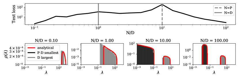
Figure 4: Empirical eigenspectrum of the covariance of the projected features ${\bm{\Sigma}}\!=\!\frac{1}{N}{\bm{Z}}^{\top}{\bm{Z}}$ at various values of $N/D$, with the corresponding test loss curve shown above. Analytics match the numerics even at $D\!=\!100$. We color the top $D$ eigenvalues in gray, which allows to separate the linear and nonlinear components at $N\!>\!D$. We set $\sigma\!=\!\mathrm{Tanh}$, $P/D=10$, $\mathrm{SNR}\!=\!0.2$, $\gamma\!=\!10^{-5}$.

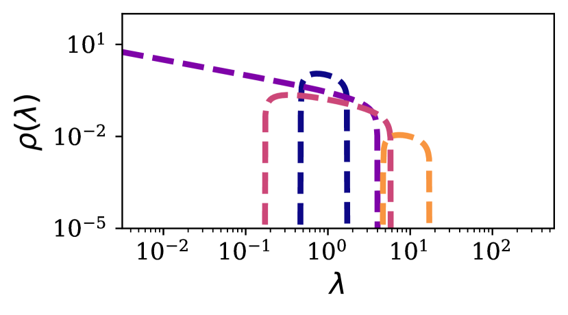
(a) Absolute value ($r\!=\!0$)

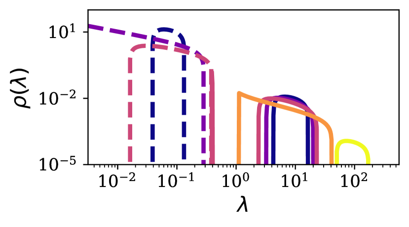
(b) Tanh ($r\!\simeq\!0.92$)

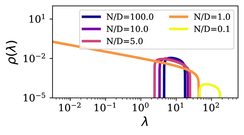
(c) Linear ($r\!=\!1$)

Figure 5: Analytical eigenspectrum of ${\bm{\Sigma}}$ for $\eta=1$, $P/D\!=\!10$, and $\zeta=0,0.92,1$ (a,b,c). We distinguish linear and nonlinear components by using respectively solid and dashed lines. (a) (purely nonlinear): the spectral gap vanishes at $N\!=\!P$ (i.e. $N/D\!=\!10$). (c) (purely linear): the spectral gap vanishes at $N\!=\!D$. (b) (intermediate): the spectral gap of the nonlinear component vanishes at $N\!=\!P$, but the gap of the linear component does not vanish at $N\!=\!D$.

In the bottom row of Fig. 4 (see also middle panel of Fig. 5), we show the numerical spectrum obtained for various values of $N/D$ with $\sigma\!=\!\mathrm{Tanh}$, and we superimpose the analytical prediction obtained from Eq. 7. At $N\!>\!D$, the spectrum separates into two components: one with $D$ large eigenvalues, and the other with $P\!-\!D$ smaller eigenvalues. The spectral gap (distance of the left edge of the spectrum to zero) closes at $N\!=\!P$, causing the nonlinear peak  [46], but remains finite at $N\!=\!D$.

Fig. 5 shows the effect of varying $r$ on the spectrum. We can interpret the results from Eq. 6:

• “Purely nonlinear” ($r\!=\!0$): this is the case of even activation functions such as $x\!\mapsto\!|x|$, which verify $\zeta\!=\!0$ according to Eq. 5. The spectrum of ${\bm{\Sigma}}_{nl}=\frac{1}{N}{\bm{W}}^{\top}{\bm{W}}$ follows a Marcenko-Pastur distribution of parameter $c=P/N$, concentrating around $\lambda\!=\!1$ at $N/D\to\infty$. The spectral gap closes at $N\!=\!P$.

• “Purely linear” ($r\!=\!1$): this is the maximal value for $r$, and is achieved only for linear networks. The spectrum of ${\bm{\Sigma}}_{l}=\frac{1}{ND}({\bm{X}}{\bm{\Theta}}^{\top})^{\top}{\bm{X}}{\bm{\Theta}}^{\top}$ follows a product Wishart distribution [47, 48], concentrating around $\lambda\!=\!P/D\!=\!10$ at $N/D\to\infty$. The spectral gap closes at $N\!=\!D$.

• Intermediate ($0\!<r\!<1$): this case encompasses all commonly used activation functions such as ReLU and Tanh. We recognize the linear and nonlinear components, which behave almost independently (they are simply shifted to the left by a factor of $r$ and $1\!-\!r$ respectively), except at $N\!=\!D$ where they interact nontrivially, leading to implicit regularization (see below).

The linear peak is implicitly regularized

As stated previously, one can expect to observe overfitting peaks when ${\bm{\Sigma}}$ is badly conditioned, i.e. its when its spectral gap vanishes. This is indeed observed in the purely linear setup at $N\!=\!D$, and in the purely nonlinear setup at $N\!=\!P$. However, in the everyday case where $0\!<\!r\!<\!1$, the spectral gap only vanishes at $N\!=\!P$, and not at $N\!=\!D$. The reason for this is that a vanishing gap is symptomatic of a random matrix reaching its maximal rank. Since $\mathrm{rk}\left({\bm{\Sigma}}_{nl}\right)=\min(N,P)$ and $\mathrm{rk}\left({\bm{\Sigma}}_{l}\right)=\min(N,P,D)$, we have $\mathrm{rk}\left({\bm{\Sigma}}_{nl}\right)\geq\mathrm{rk}\left({\bm{\Sigma}}_{l}\right)$ at $P\!>\!D$. Therefore, the rank of ${\bm{\Sigma}}$ is imposed by the nonlinear component, which only reaches its maximal rank at $N\!=\!P$. At $N\!=\!D$, the nonlinear component acts as an implicit regularization, by compensating the small eigenvalues of the linear component. This causes the linear peak to be implicitly regularized be the presence of the nonlinearity.

What is the linear peak caused by?

At $0\!<\!r\!<\!1$, the spectral gap vanishes at $N\!=\!P$, causing the norm of the estimator $\|{\bm{a}}\|$ to peak, but it does not vanish at $N\!=\!D$ due to the implicit regularization; in fact, the lowest eigenvalue of the full spectrum does not even reach a local minimum at $N\!=\!D$. Nonetheless, a soft linear peak remains as a vestige of what happens at $r=1$. What is this peak caused by? A closer look at the spectrum of Fig. 5.b clarifies this question. Although the left edge of the full spectrum is not minimal at $N\!=\!D$, the left edge of the linear component, in solid lines, reaches a minimum at $N\!=\!D$. This causes a peak in $\|{\bm{\Theta}}{\bm{a}}\|$, the norm of the “linearized network”, as shown in Sec. B of the SM. This, in turn, entails a different kind of overfitting as we explain in the next section.

2.3 Bias-variance decomposition

The previous spectral analysis suggests that both peaks are related to some kind of overfitting. To address this issue, we make use of the bias-variance decomposition presented in [20]. The test loss is broken down into four contributions: a bias term and three variance terms stemming from the randomness of (i) the random feature vectors ${\bm{\Theta}}$ (which plays the role of initialization variance in realistic networks), (ii) the noise ${\bm{\epsilon}}$ corrupting the labels of the training set (noise variance) and (iii) the inputs ${\bm{X}}$ (sampling variance). We defer to [20] for further details.

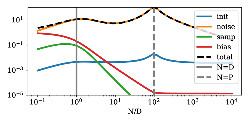
(a) Vanilla

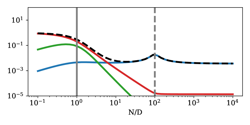
(b) Noiseless

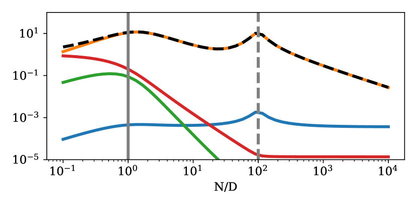
(c) Ensembling

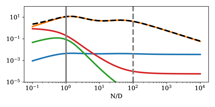
(d) Regularizing

Figure 6: Bias-variance decompostion of the test loss in the RF model for $\sigma=\mathrm{ReLU}$ and $P/D=100$. Regularizing (increasing $\gamma$) and ensembling (increasing the number $K$ of initialization seeds we average over) mitigates the nonlinear peak but does not affect the linear peak. (a) $K\!=\!1,\gamma\!=\!10^{-5},SNR\!=\!0.2$. (b) Same but $SNR\!=\!\infty$. (c) Same but $K=10$. (d) Same but $\gamma=10^{-3}$.

Only the nonlinear peak is affected by initialization variance

In Fig. 6.a, we show such a decomposition. As observed in [20], the nonlinear peak is caused by an interplay between initialization and noise variance. This peak appears starkly at $N\!=\!P$ in the high noise setup, where noise variance dominates the test loss, but also in the noiseless setup (Fig. 6.b), where the residual initialization variance dominates: nonlinear networks can overfit even in absence of noise.

The linear peak vanishes in the noiseless setup

In stark contrast, the linear peak which appears clearly at $N\!=\!D$ in Fig. 6.a is caused solely by a peak in noise variance, in agreement with [6]. Therefore, it vanishes in the noiseless setup of Fig. 6.b. This is expected, as for linear networks the solution to the minimization problem is independent of the initialization of the weights.

3 Phenomenology of triple descent

3.1 The nonlinearity determines the relative height of the peaks

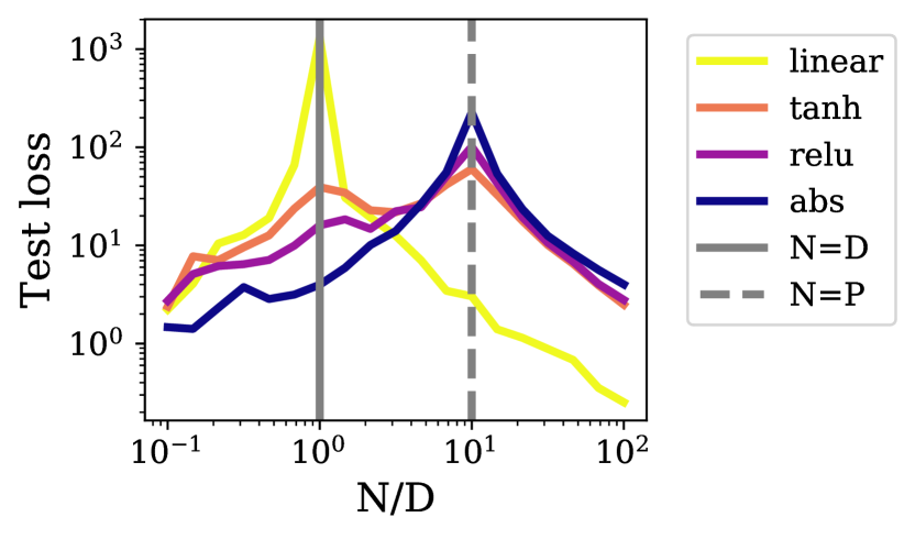
Figure 7: Numerical test loss of RF models at finite size ($D=100$), averaged over 10 runs. We set $P/D=10$, $\mathrm{SNR}=0.2$ and $\gamma=10^{-3}$.

In Fig. 7, we consider RF models with four different activation functions: absolute value ($r=0$), ReLU ($r=0.5$), Tanh ($r\sim 0.92$) and linear ($r=1$). We see that increasing the degree of nonlinearity strengthens the nonlinear peak (by increasing initialization variance) and weakens the linear peak (by increasing the implicit regularization). In Sec. A of the SM, we present additional results where the degree of linearity $r$ is varied systematically in the RF model, and show that replacing Tanh by ReLU in the NN setup produces a similar effect. Note that the behavior changes abruptly near $r=1$, marking the transition to the linear regime.

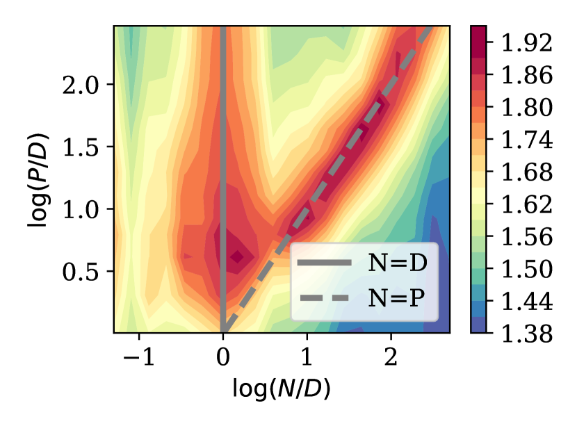
(a) Vanilla

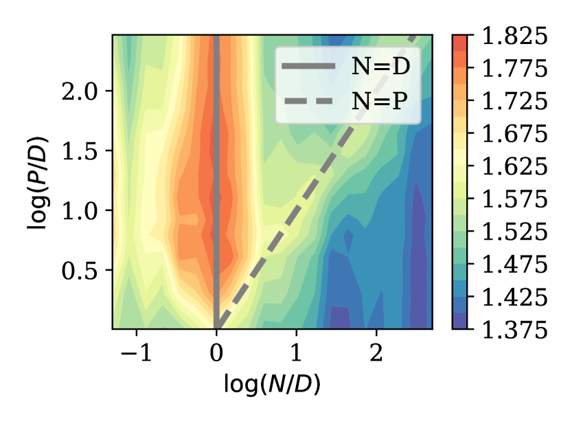
(b) Ensembling

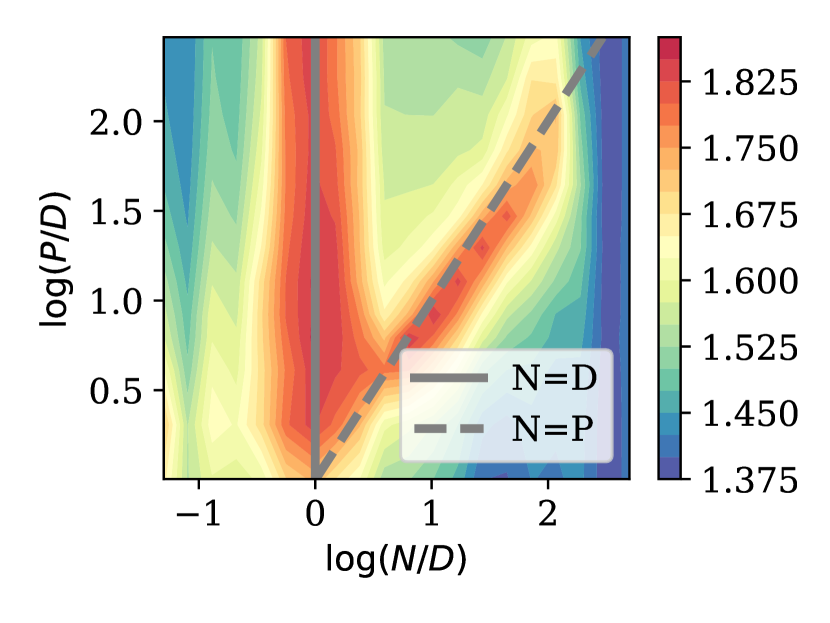
(c) Regularizing

Figure 8: Test loss phase space for the NN model with $\sigma=\mathrm{Tanh}$. Weight decay with parameter $\gamma$ and ensembling over $K$ seeds weakens the nonlinear peak but leaves the linear peak untouched. (a) $K\!=\!1,\gamma\!=\!0,SNR\!=\!0.2$. (b) Same but $K=10$. (c) Same but $\gamma=0.05$.

3.2 Ensembling and regularization only affects the nonlinear peak

It is a well-known fact that regularization [19] and ensembling [9, 20, 49] can mitigate the nonlinear peak. This is shown in panel (c) and (d) of Fig. 6 for the RF model, where ensembling is performed by averaging the predictions of 10 RF models with independently sampled random feature vectors. However, we see that these procedures only weakly affect the linear peak. This can be understood by the fact that the linear peak is already implicitly regularized by the nonlinearity for $r<1$, as explained in Sec. 2.

In the NN model, we perform a similar experiment by using weight decay as a proxy for the regularization procedure, see Fig. 8. Similarly as in the RF model, both ensembling and regularizing attenuates the nonlinear peak much more than the linear peak.

3.3 The nonlinear peak forms later during training

To study the evolution of the phase space during training dynamics, we focus on the NN model (there are no dynamics involved in the RF model we considered, where the second layer weights were learnt via ridge regression). In Fig. 9, we see that the linear peak appears early during training and maintains throughout, whereas the nonlinear peak only forms at late times. This can be understood qualitatively as follows [6]: for linear regression the time required to learn a mode of eigenvalue $\lambda$ in the covariance matrix is proportional to $\lambda^{-1}$. Since the nonlinear peak is due to vanishingly small eigenvalues, which is not the case of the linear peak, the nonlinear peak takes more time to form completely.

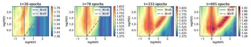
Figure 9: Test loss phase space for the NN model with $\sigma=\mathrm{Tanh}$, plotted at various times during training. The linear peak grows first, followed by the nonlinear peak.

4 Conclusion

One of the key challenges in solving tasks with network-like architectures lies in choosing an appropriate number of parameters $P$ given the properties of the training dataset, namely its size $N$ and dimension $D$. By elucidating the structure of the $(P,N)$ phase space, its dependency on $D$, and distinguishing the two different types of overfitting which it can exhibit, we believe our results can be of interest to practitioners.

Our results leave room for several interesting follow-up questions, among which the impact of (1) various architectural choices, (2) the optimization algorithm, and (3) the structure of the dataset. For future work, we will consider extensions along those lines with particular attention to the structure of the dataset. We believe it will provide a deeper insight into data-model matching.

Acknowledgements

We thank Federica Gerace, Armand Joulin, Florent Krzakala, Bruno Loureiro, Franco Pellegrini, Maria Refinetti, Matthieu Wyart and Lenka Zdeborova for insightful discussions. GB acknowledges funding from the French government under management of Agence Nationale de la Recherche as part of the "Investissements d’avenir" program, reference ANR-19-P3IA-0001 (PRAIRIE 3IA Institute) and from the Simons Foundation collaboration Cracking the Glass Problem (No. 454935 to G. Biroli).

Broader Impact

Due to the theoretical nature of this paper, a Broader Impact discussion is not easily applicable. However, given the tight interaction of data & model and their impact on overfitting regimes, we believe that our findings and this line of research, in general, may potentially impact how practitioners deal with data.

Appendix A Effect of signal-to-noise ratio and nonlinearity

A.1 RF model

In the RF model, varying $r$ can easily be achieved analytically and yields interesting results, as shown in Fig. 10.

In the top panel, we see that the parameter-wise profile exhibits double descent for all degrees of linearity $r$ and signal-to-noise ratio $\mathrm{SNR}$, except in the linear case $r=1$ which is monotonously deceasing. Increasing the degree of nonlinearity (decreasing $r$) and the noise (decreasing the $\mathrm{SNR}$) simply makes the nonlinear peak stronger.

In the bottom panel, we see that the sample-wise profile is more complex. In the linear case $r=1$, only the linear peak appears (except in the noiseless case). In the nonlinear case $r<1$, the nonlinear peak appears is always visible; as for the linear peak, it is regularized away, except in the strong noise regime $\mathrm{SNR}>1$ when the degree of nonlinearity is small ($r>0.8$), where we observe the triple descent.

Notice that both in the parameter-wise and sample-wise profiles, the test loss profiles change smoothly with $r$, except near $r=1$ where the behavior abruptly changes, particularly at low $\mathrm{SNR}$.

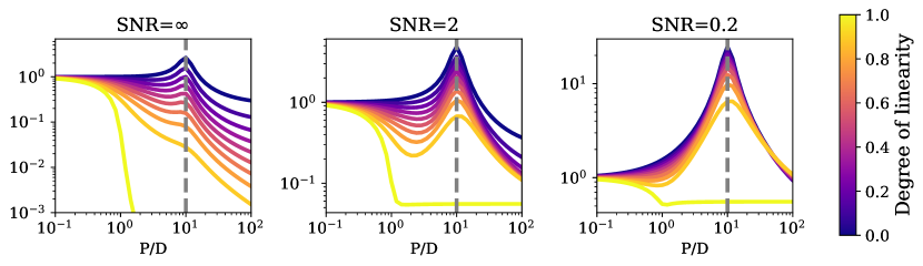
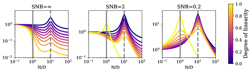
Figure 10: Analytical parameter-wise (top, $N/D=10$) and sample-wise (bottom, $P/D=10$) test loss profiles of the RF model. Left: noiseless case, $\mathrm{SNR}=\infty$. Center: low noise, $\mathrm{SNR}=2$. Right: high noise, $\mathrm{SNR}=0.2$. We set $\gamma=10^{-1}$.

One can also mimick these results numerically by considering, as in [38], the following family of piecewise linear functions:

$$\sigma_{\alpha}(x)=\frac{[x]_{+}+\alpha[-x]_{+}-\frac{1+\alpha}{\sqrt{2\pi}}}{\sqrt{\frac{1}{2}\left(1+\alpha^{2}\right)-\frac{1}{2\pi}(1+\alpha)^{2}}},$$ (8)

for which

$$r_{\alpha}=\frac{(1-\alpha)^{2}}{2\left(1+\alpha^{2}\right)-\frac{2}{\pi}(1+\alpha)^{2}}.$$ (9)

Here, $\alpha$ parametrizes the ratio of the slope of the negative part to the positive part and allows to adjust the value of $r$ continuously. $\alpha=-1$ ($r=1$) will correspond to a (shifted) absolute value, $\alpha=1$ ($r=0$) will correspond to a linear function, $\alpha=0$ will correspond to a (shifted) ReLU. In Fig. 11, we show the effect of sweeping $\alpha$ uniformly from 1 to -1 (which causes $r$ to range from 0 to 1). As expected, we see the linear peak become stronger and the nonlinear peak become weaker.

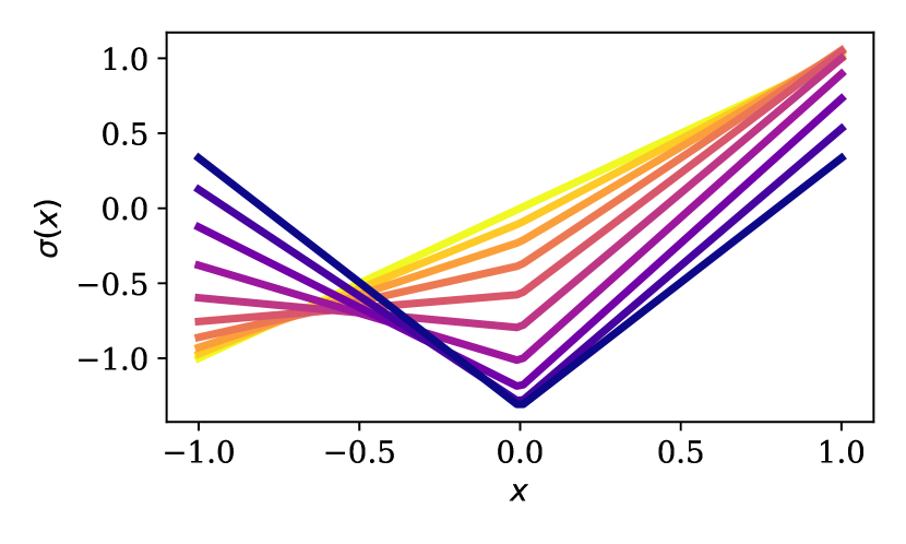
(a) Nonlinearities used

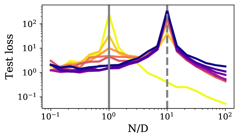
(b) Corresponding test loss

Figure 11: Moving from a purely nonlinear function to a purely linear function (dark to light colors) strengthens the linear peak and weakens the nonlinear peak.

A.2 NN model

In Fig. 12, we show the effect of replacing Tanh ($r\sim 0.92$) by ReLU ($r=0.5$). We still distinguish the two peaks of triple descent, but the linear peak is much weaker in the case of ReLU, as expected from the stronger degree of nonlinearity.

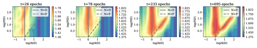
(a) Tanh

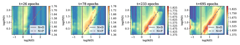
(b) ReLU

Figure 12: Dynamics of the test loss phase space, with weight decay $\gamma=0.05$. Top: Tanh. Bottom: ReLU.

Appendix B Origin of the linear peak

In this section, we follow the lines of [37], where the test loss is decomposed in the following way (Eq. D.6):

$$\mathcal{L}_{g}=\rho+Q-2M$$ (10)

$$\rho=\frac{1}{D}\left\|\bm{\beta}\right\|^{2},\quad M=\frac{\sqrt{\zeta}}{D}{\bm{b}}\cdot\bm{\beta},\quad Q=\frac{\zeta}{D}\|{\bm{b}}\|^{2}+\frac{\eta-\zeta}{P}\|{\bm{a}}\|^{2},\quad{\bm{b}}={\bm{\Theta}}{\bm{a}}$$ (11)

As before, ${\bm{\beta}}$ denotes the linear teacher vector and ${\bm{\Theta}},{\bm{a}}$ respectively denote the (fixed) first and (learnt) second layer of the student. This insightful expression shows that the loss only depends on the norm of the second layer $\|{\bm{a}}\|$, the norm of the linearized network $\|{\bm{b}}\|$, and its overlap with the teacher ${\bm{b}}\cdot\bm{\beta}$.

We plot these three terms in Fig. 13, focusing on the triple descent scenario $\mathrm{SNR}<1$. In the left panel, we see that the overlap of the student with the teacher is monotically increasing, and reaches its maximal value at a certain point which increases from $D$ to $P$ as we decrease $r$ from 1 to 0. In the central panel, we see that $\|{\bm{a}}\|$ peaks at $N=P$, causing the nonlinear peak as expected, but nothing special happens at $N=D$ (except for $r=1$). However, in the right panel, we see that the norm of the linearized network peaks at $N=D$, where we know from the spectral analysis that the gap of the linear part of the spectrum is minimal. This is the origin of the linear peak.

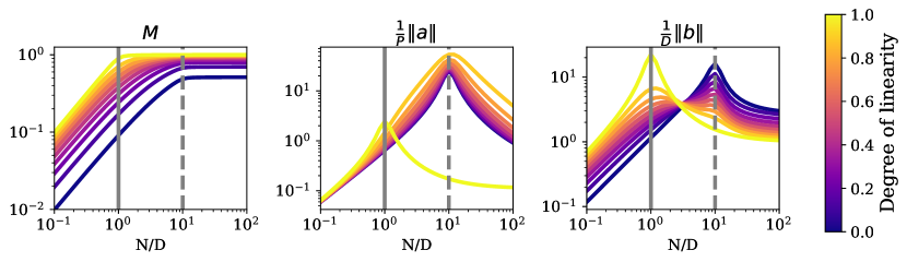
Figure 13: Terms entering Eq. 11, plotted at $\mathrm{SNR}=0.2$, $\gamma=10^{-1}$.

Appendix C Structured datasets

In this section, we examine how our results are affected by considering the realistic case of correlated data. To do so, we replace the Gaussian i.i.d. data by MNIST data, downsampled to $10\times 10$ images for the RF model ($D=100$) and $14\times 14$ images for the NN model ($D=196$).

C.1 RF model: data structure does not matter in the lazy regime

We refer to the results in Fig 14. Interestingly, the triple descent profile is weakly affected by the correlated structure of this realistic dataset: the linear peak and nonlinear peaks still appear, respectively at $N=D$ and $N=P$. However, the spectral properties of ${\bm{\Sigma}}=\frac{1}{N}{\bm{Z}}^{\top}{\bm{Z}}$ are changed in an interesting manner: the two parts of the spectrum are now contiguous, there is no gap between the linear part and the nonlinear part.

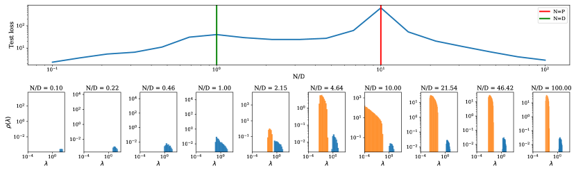
(a) Random data

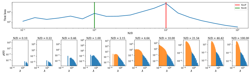
(b) MNIST

Figure 14: Spectrum of the covariance of the projected features ${\bm{\Sigma}}=\frac{1}{N}{\bm{Z}}^{\top}{\bm{Z}}$ at various values of $N/D$, with the corresponding loss curve shown above. We set $\sigma=\mathrm{Tanh}$, $\gamma=10^{-5}$.

C.2 NN model: the effect of feature learning

As shown in Fig. 15, the NN model behaves very differently on structured data like CIFAR10. At late times, three main differences with respect to the case of random data can be observed in the low $\mathrm{SNR}$ setup:

• Instead of a clearly defined linear peak at $N=D$, we observe a large overfitting regions at $N<D$.

• The nonlinear peak shifts to higher values of $N$ during time, but always scales sublinearly with $P$, i.e. it is located at $N\sim P^{\alpha}$ with $\alpha<1$

Behavior of the linear peaks

As emphasized by [35], a non-trivial structure of the covariance of the input data can strongly affect the number and location of linear peaks. For example, in the context of linear regression, [19] considers gaussian data drawn from a diagonal covariance matrix $\Sigma\in\mathbb{R}^{30\times 30}$ with two blocks of different strengths: $\Sigma_{i},i=10$ for $i\leq 15$ and $\Sigma_{i},i=1$ for $i\geq 15$. In this situation, two linear peaks are observed: one at $N_{1}=15$, and one at $N_{2}=30$. In the setup of structured data such as CIFAR10, where the covariance is evidently much more complicated, one can expect to see a multiple peaks, all located at $N\leq D$.

This is indeed what we observe: in the case of Tanh, where the linear peaks are strong, two linear peaks are particularly at late times, at $N_{1}=10^{-1.5}D$, and the other at $N_{2}=10^{-2}D$. In the case of ReLU, they are obscured at late times by the strength of the nonlinear peak.

Behavior of the nonlinear peak

We observe that during training, the nonlinear peak shifts towards higher values of $N$. This phenomenon was already observed in [12], where it is explained through the notion of effective model complexity. The intuition goes as follows: increasing the training time increases the expressivity of a given model, and therefore increases the number of training examples it can overfit.

We argue that this sublinear scaling is a consequence of the fact that structured data is easier to memorize than random data [18]: as the dataset grows large, each new example becomes easier to classify since the network has learnt the underlying rule (in contrast to the case of random data where each new example makes the task harder by the same amount).

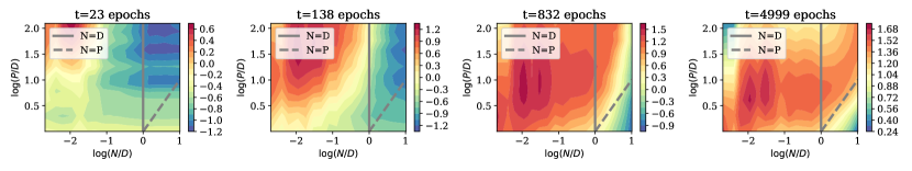
(a) CIFAR10, Tanh

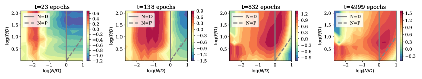
(b) CIFAR10, ReLU

Figure 15: Dynamics of test loss phase space on CIFAR10 with $\mathrm{SNR}=0.2$, for different activation functions.

References

- [1] Alex Krizhevsky, Ilya Sutskever, and Geoffrey E Hinton. Imagenet classification with deep convolutional neural networks. In Advances in neural information processing systems, pages 1097–1105, 2012.
- [2] Yann LeCun, Yoshua Bengio, and Geoffrey Hinton. Deep learning. nature, 521(7553):436–444, 2015.
- [3] Geoffrey Hinton, Li Deng, Dong Yu, George E Dahl, Abdel-rahman Mohamed, Navdeep Jaitly, Andrew Senior, Vincent Vanhoucke, Patrick Nguyen, Tara N Sainath, et al. Deep neural networks for acoustic modeling in speech recognition: The shared views of four research groups. IEEE Signal processing magazine, 29(6):82–97, 2012.
- [4] Ilya Sutskever, Oriol Vinyals, and Quoc V Le. Sequence to sequence learning with neural networks. In Advances in neural information processing systems, pages 3104–3112, 2014.
- [5] Chiyuan Zhang, Samy Bengio, Moritz Hardt, Benjamin Recht, and Oriol Vinyals. Understanding deep learning requires rethinking generalization. arXiv preprint arXiv:1611.03530, 2016.
- [6] Madhu S Advani and Andrew M Saxe. High-dimensional dynamics of generalization error in neural networks. arXiv preprint arXiv:1710.03667, 2017.
- [7] Behnam Neyshabur, Zhiyuan Li, Srinadh Bhojanapalli, Yann LeCun, and Nathan Srebro. Towards understanding the role of over-parametrization in generalization of neural networks. arXiv preprint arXiv:1805.12076, 2018.
- [8] Mikhail Belkin, Daniel Hsu, Siyuan Ma, and Soumik Mandal. Reconciling modern machine learning and the bias-variance trade-off. arXiv preprint arXiv:1812.11118, 2018.
- [9] Mario Geiger, Arthur Jacot, Stefano Spigler, Franck Gabriel, Levent Sagun, Stéphane d’Ascoli, Giulio Biroli, Clément Hongler, and Matthieu Wyart. Scaling description of generalization with number of parameters in deep learning. Journal of Statistical Mechanics: Theory and Experiment, 2020(2):023401, 2020.
- [10] S Spigler, M Geiger, S d’Ascoli, L Sagun, G Biroli, and M Wyart. A jamming transition from under-to over-parametrization affects generalization in deep learning. Journal of Physics A: Mathematical and Theoretical, 52(47):474001, 2019.
- [11] Song Mei and Andrea Montanari. The generalization error of random features regression: Precise asymptotics and double descent curve. arXiv preprint arXiv:1908.05355, 2019.
- [12] Preetum Nakkiran, Gal Kaplun, Yamini Bansal, Tristan Yang, Boaz Barak, and Ilya Sutskever. Deep double descent: Where bigger models and more data hurt. arXiv preprint arXiv:1912.02292, 2019.
- [13] Preetum Nakkiran. More data can hurt for linear regression: Sample-wise double descent. arXiv preprint arXiv:1912.07242, 2019.
- [14] Manfred Opper and Wolfgang Kinzel. Statistical mechanics of generalization. In Models of neural networks III, pages 151–209. Springer, 1996.
- [15] Andreas Engel and Christian Van den Broeck. Statistical mechanics of learning. Cambridge University Press, 2001.
- [16] Florent Krzakala and Jorge Kurchan. Landscape analysis of constraint satisfaction problems. Physical Review E, 76(2):021122, 2007.
- [17] Silvio Franz and Giorgio Parisi. The simplest model of jamming. Journal of Physics A: Mathematical and Theoretical, 49(14):145001, 2016.
- [18] Mario Geiger, Stefano Spigler, Stéphane d’Ascoli, Levent Sagun, Marco Baity-Jesi, Giulio Biroli, and Matthieu Wyart. Jamming transition as a paradigm to understand the loss landscape of deep neural networks. Physical Review E, 100(1):012115, 2019.
- [19] Preetum Nakkiran, Prayaag Venkat, Sham Kakade, and Tengyu Ma. Optimal regularization can mitigate double descent. arXiv preprint arXiv:2003.01897, 2020.
- [20] Stéphane d’Ascoli, Maria Refinetti, Giulio Biroli, and Florent Krzakala. Double trouble in double descent: Bias and variance (s) in the lazy regime. arXiv preprint arXiv:2003.01054, 2020.
- [21] Yann Le Cun, Ido Kanter, and Sara A Solla. Eigenvalues of covariance matrices: Application to neural-network learning. Physical Review Letters, 66(18):2396, 1991.
- [22] Anders Krogh and John A Hertz. Generalization in a linear perceptron in the presence of noise. Journal of Physics A: Mathematical and General, 25(5):1135, 1992.
- [23] Robert PW Duin. Small sample size generalization. In Proceedings of the Scandinavian Conference on Image Analysis, volume 2, pages 957–964. PROCEEDINGS PUBLISHED BY VARIOUS PUBLISHERS, 1995.
- [24] Trevor Hastie, Andrea Montanari, Saharon Rosset, and Ryan J Tibshirani. Surprises in high-dimensional ridgeless least squares interpolation. arXiv preprint arXiv:1903.08560, 2019.
- [25] Melikasadat Emami, Mojtaba Sahraee-Ardakan, Parthe Pandit, Sundeep Rangan, and Alyson K Fletcher. Generalization error of generalized linear models in high dimensions. arXiv preprint arXiv:2005.00180, 2020.
- [26] Benjamin Aubin, Florent Krzakala, Yue M Lu, and Lenka Zdeborová. Generalization error in high-dimensional perceptrons: Approaching bayes error with convex optimization. arXiv preprint arXiv:2006.06560, 2020.
- [27] Zeng Li, Chuanlong Xie, and Qinwen Wang. Provable more data hurt in high dimensional least squares estimator. arXiv preprint arXiv:2008.06296, 2020.
- [28] Andrew M Saxe, James L McClelland, and Surya Ganguli. Exact solutions to the nonlinear dynamics of learning in deep linear neural networks. arXiv preprint arXiv:1312.6120, 2013.
- [29] Andrew K Lampinen and Surya Ganguli. An analytic theory of generalization dynamics and transfer learning in deep linear networks. arXiv preprint arXiv:1809.10374, 2018.
- [30] Ali Rahimi and Benjamin Recht. Random features for large-scale kernel machines. In Advances in neural information processing systems, pages 1177–1184, 2008.
- [31] Marco Loog and Robert PW Duin. The dipping phenomenon. In Joint IAPR International Workshops on Statistical Techniques in Pattern Recognition (SPR) and Structural and Syntactic Pattern Recognition (SSPR), pages 310–317. Springer, 2012.
- [32] Marco Loog, Tom Viering, and Alexander Mey. Minimizers of the empirical risk and risk monotonicity. In Advances in Neural Information Processing Systems, pages 7478–7487, 2019.
- [33] Yifei Min, Lin Chen, and Amin Karbasi. The curious case of adversarially robust models: More data can help, double descend, or hurt generalization. arXiv preprint arXiv:2002.11080, 2020.
- [34] Tengyuan Liang, Alexander Rakhlin, and Xiyu Zhai. On the risk of minimum-norm interpolants and restricted lower isometry of kernels. arXiv preprint arXiv:1908.10292, 2019.
- [35] Lin Chen, Yifei Min, Mikhail Belkin, and Amin Karbasi. Multiple descent: Design your own generalization curve. arXiv preprint arXiv:2008.01036, 2020.
- [36] Ben Adlam and Jeffrey Pennington. The neural tangent kernel in high dimensions: Triple descent and a multi-scale theory of generalization. arXiv preprint arXiv:2008.06786, 2020.
- [37] Federica Gerace, Bruno Loureiro, Florent Krzakala, Marc Mézard, and Lenka Zdeborová. Generalisation error in learning with random features and the hidden manifold model. arXiv preprint arXiv:2002.09339, 2020.
- [38] Jeffrey Pennington and Pratik Worah. Nonlinear random matrix theory for deep learning. In Advances in Neural Information Processing Systems, pages 2637–2646, 2017.
- [39] Arthur Jacot, Franck Gabriel, and Clément Hongler. Neural tangent kernel: Convergence and generalization in neural networks. In Advances in neural information processing systems, pages 8571–8580, 2018.
- [40] Lénaïc Chizat, Edouard Oyallon, and Francis Bach. On lazy training in differentiable programming. In H. Wallach, H. Larochelle, A. Beygelzimer, F. d’Alché Buc, E. Fox, and R. Garnett, editors, Advances in Neural Information Processing Systems 32, pages 2933–2943. Curran Associates, Inc., 2019.
- [41] S Péché et al. A note on the pennington-worah distribution. Electronic Communications in Probability, 24, 2019.
- [42] Sebastian Goldt, Galen Reeves, Marc Mézard, Florent Krzakala, and Lenka Zdeborová. The gaussian equivalence of generative models for learning with two-layer neural networks. arXiv preprint arXiv:2006.14709, 2020.
- [43] Lucas Benigni and Sandrine Péché. Eigenvalue distribution of nonlinear models of random matrices. arXiv preprint arXiv:1904.03090, 2019.
- [44] Ben Adlam, Jake Levinson, and Jeffrey Pennington. A random matrix perspective on mixtures of nonlinearities for deep learning. arXiv preprint arXiv:1912.00827, 2019.
- [45] Zhenyu Liao and Romain Couillet. On the spectrum of random features maps of high dimensional data. arXiv preprint arXiv:1805.11916, 2018.
- [46] Madhu Advani, Subhaneil Lahiri, and Surya Ganguli. Statistical mechanics of complex neural systems and high dimensional data. Journal of Statistical Mechanics: Theory and Experiment, 2013(03):P03014, 2013.
- [47] Thomas Dupic and Isaac Pérez Castillo. Spectral density of products of wishart dilute random matrices. part i: the dense case. arXiv preprint arXiv:1401.7802, 2014.
- [48] Gernot Akemann, Jesper R Ipsen, and Mario Kieburg. Products of rectangular random matrices: singular values and progressive scattering. Physical Review E, 88(5):052118, 2013.
- [49] Andrew Gordon Wilson and Pavel Izmailov. Bayesian deep learning and a probabilistic perspective of generalization. arXiv preprint arXiv:2002.08791, 2020.