Generating a tide-like flow in a cylindrical vessel by electromagnetic forcing

Abstract

We show and compare numerical and experimental results on the electromagnetic generation of a tide-like flow structure in a cylindrical vessel which is filled with the eutectic liquid metal alloy GaInSn. Fields of various strengths and frequencies are applied to drive liquid metal flows. The impact of the field variations on amplitude and structure of the flows are investigated. The results represent the basis for a future Rayleigh-Bénard experiment, in which a modulated tide-like flow perturbation is expected to synchronize the typical sloshing mode of the large-scale circulation. A similar entrainment mechanism for the helicity in the Sun may be responsible for the synchronization of the solar dynamo with the alignment cycle of the tidally dominant planets Venus, Earth and Jupiter.

I Introduction

In a series of recent papers Weber2015 ; Stefani2016 ; Stefani2018 ; Stefani2019 ; Stefani2020 , an attempt was made to explain the remarkable empirical synchronization of the solar cycle with the 11.07 years alignment cycle of the tidally dominant planets Venus, Earth and Jupiter. The basic idea relies, first, on the tendency of the current-driven, kink-type ($m=1$) Tayler instability (TI) Tayler1973 to undergo helicity oscillations Weber2015 and, second, on the fact that these helicity oscillations can easily be entrained by tide-like forces with their typical $m=2$ azimuthal dependence Stefani2016 . While the tidal forces of the planets are indeed tiny, in this mechanism they are only needed as a catalyst to switch between left- and right-handed states of the TI, without, or just barely, changing its energy content.

This theory is still highly speculative and further conceptual and numerical work will be needed for its verification. Additional experimental insight into this synchronization effect could also be helpful in this respect. Unfortunately, experiments on the very TI using liquid metals (which are, similarly as the plasma in the solar tachocline region, characterized by a low magnetic Prandtl number) have turned out especially complicated Seilmayer2012 , mainly due to the necessity to characterize the instability in a contactless manner in order not to generate any interfering electrovortex flow by the insertion of measurement probes such as ultrasonic transducers.

Yet, the key idea of synchronizing the helicity, which is connected with an $m=1$ flow structure, by some tide-like $m=2$ perturbation might have wider applicability than just for the TI case. An interesting candidate in this respect is the $m=1$ magneto-Rossby wave at the solar tachoclineDikpati2017 ; McIntosh2017 ; Tobias2017 ; Zaqarashvili2018 , which could open up a complementary route for synchronizing the solar dynamo by tidal forces.

Large-scale circulation (LSC) Krishnamurti1981 ; Sano1989 ; Takeshita1996 ; Cioni1997 ; XiLamXia2004 ; BrownAhlers2006 ; Resagk2006 ; Xi2008 , which appears in Rayleigh-Bénard convection (RBC) when thermal plumes erupt from the boundary layer and self-organize into a flywheel structure Kadanoff2001 , is another candidate. Quite similarly as the TI, the $m=1$ LSC also breaks spontaneously the axi-symmetry ($m=0$) of the underlying problem, and becomes prone to secondary effects such as torsional Funfschilling2004 and sloshing modes XiZhou2009 ; BrownAhlers2009 , reversals and even intermittent cessations BrownAhlers2006 ; Xi2008 . Experiments on the LSC problem were carried out with different working fluids, including water Krishnamurti1981 ; BrownAhlers2006 ; Xi2008 , silicon oil Krishnamurti1981 , helium-gas Sano1989 , air Resagk2006 , liquid mercury Takeshita1996 ; Cioni1997 , liquid sodium Khalilov2018 , and the eutectic alloy GaInSn Wondrak2018 ; Zuerner2019 .

On closer consideration, the sloshing mode with its side-wise motion transverse to the primary LSC vortex, turns out to be connected with helicity oscillations. Some preliminary simulations have recently shown that this sloshing motion of the LSC can also be synchronized by an $m=2$ perturbation, although with a different frequency relation (2:1) than in the TI-case. This effect, which might have to do with the different numbers of vertically stacked vortices, needs further clarification. At any rate, the interaction of the sloshing mode of an LSC with some $m=2$ perturbation seems quite promising for experimentally evidencing the generic effect of helicity synchronization by tide-like forces.

There are different ways to experimentally realize such perturbations. In a zonal wind experiment, for example, a deformable wall was used to force a tide-like perturbation Morize2010 . When using a liquid metal, electromagnetic forcing, modulated in time, opens an alternative route for realizing an $m=2$ flow perturbation. Such a concept of tide-like forcing will be pursued in this paper, where we focus, though, mainly on the spatial ($m=2$) aspect of the tidal flow, leaving its time-dependence and its influence on the LSC to future studies.

Our experiment utilizes the versatile MULTIMAG system Pal2009 , which allows for arbitrary superpositions of axial, rotating, and travelling magnetic fields. In a recent paper StepanovStefani2019 , various combinations of the six coils, which are normally used for producing the rotating magnetic field (RMF), have been evaluated with respect to their suitability to generate a typical tide-like $m=2$ flow perturbation. Although these preparatory simulations were made in the simple Stokes approximation, they were indeed useful to discriminate between different flow topologies when applying various combinations of the available coils. A very favourable flow structure appeared for the comparably simple configuration that two oppositely situated coils are fed with AC currents with a frequency of some tens of Hz.

Based on this prediction, we have carried out a corresponding experiment in which we measured the electromagnetically driven $m=2$ flow in a vessel filled with the eutectic alloy GaInSn. We will show that the measured flow structure corresponds well with the results of accompanying OpenFOAM^© simulations. This gives a solid basis for the combination of a LSC flow produced by thermal convection with a modulated $m=2$ force, which is planned for further experiments.

II Experimental setup

The experiments were performed in a cylindrical container with inner diameter $D=2R=$180 mm and aspect ratio $\Gamma=D/H=1$, where $H$ is the height. On top and bottom, the cylinder is bounded by two 220 mm diameter, 25 mm thick uncoated copper plates. The sidewalls consist of polyether ether ketone (PEEK). The cell is filled with the liquid metal alloy GaInSn with Prandtl number Pr$=0.029$. Other relevant physical parameters at $20^{\circ}$ C are Plevachuk2015 : density $\rho=6350$ kg/m³, kinematic viscosity $\nu=3.44\times 10^{-7}$ m²/s, and electrical conductivity $\sigma=3.27\times 10^{6}$ ($\Omega$ m)^-1. From the latter two values, we derive a magnetic Prandtl number $Pm=\mu_{0}\sigma\nu=1.40\times 10^{-6}$.

The configuration of sensor placements is illustrated in Fig. 1. To measure the radial velocities, eight Ultrasound Doppler Velocimetry (UDV) sensors are located at three different heights in the sidewall of the cell. They have a flat head, 8 mm in diameter and are excited with 7.8-8 MHz pulses. The sampling time for one velocity profile is 2.7$\pm$0.2 s, if not stated otherwise. Starting from the bottom boundary between copper and the liquid alloy, the measurement planes “Bot”, “Mid” and “Top” are located at heights of 10, 90 and 170 mm, respectively. At each height, two sensors called “1” and “3” are placed with an angle of $\pi/2$ between them. Additionally, the “Top” and “Bot” levels each have an additional sensor “2” at the bisection between sensors “1” and “3”. Two further UDV sensors for measuring the vertical flow component are placed in the top copper plate at radial positions $r/R=0$ and $r/R=0.8$. A more detailed description of the cell can be found in Zuerner2019 .

The $m=2$ flow is driven by AC-currents through two rectangular, stretched coils which are situated on opposite sides of the cylinder as delineated in Fig. 1. They consist of 80 turns each with a total inner height of 450 mm and an average distance between the long leg and the x-z centre plane of 145 mmPal2009 . When a current is run through the coils a magnetic field is generated, which is symmetrical to this centre plane. A tunable AC power supply is used to create an alternating current with defined amplitude and frequency in the coils. The polarity of the coils is assigned in a way that the magnetic field is concordant in both solenoids. This configuration has turned out advantageous for generating the desired flow fieldStepanovStefani2019 . For the case that the vessel is not installed, the correlation of the measured flux density and the applied coil current is depicted in Fig. 2.

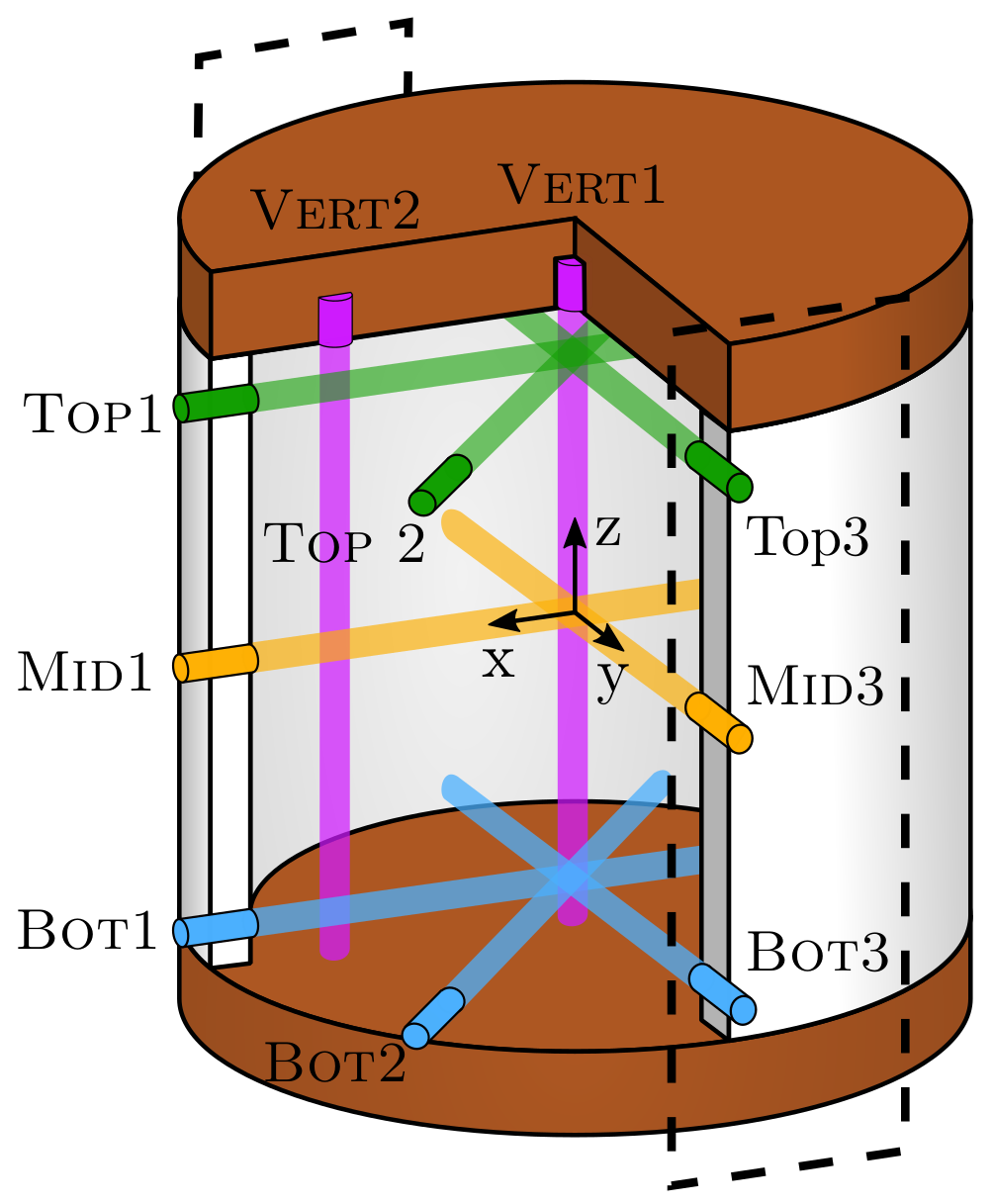
Figure 1: Schematic setup of the experimental cell showing the UDV sensor placement and the measurement paths. The arrangement of the excitation coils lying on the y-axis is indicated by the dashed lines.

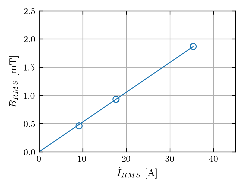
Figure 2: RMS magnetic flux density at 25 Hz in the centre of MultiMAG depending on the RMS value of the AC current. The experimental cell was not installed during this measurement.

For the particular choice of an AC-current with RMS value 9 A and a frequency of 25 Hz, Fig. 3 shows an exemplary measurement result of sensor Mid1, i.e. the sensor at mid-height with beamline in $x$-direction which is perpendicular to the $y$-axis (connecting the two excitation coils). In principle, this measurement shows a flow that is directed away from the walls, leading to a positive projection (red) onto the ultrasound beam for lower distances, and to a negative projection (blue) for higher distances from the UDV sensor. Not surprisingly, the resulting stagnation point is rather unstable, leading to a “restless” behaviour of the flow.

Nevertheless, we can define a time average for all the profiles measured during this run, which yields a sinusoidal dependence on the depth of the ultrasound beam (Fig. 4), with a peak-to-peak amplitude $\hat{v}\sim 7$ mm/s in this specific case. Every measurement encompasses between 1300 and 1500 profiles which, in turn, are averages over 100 to 250 UDV emissions (typically 150).

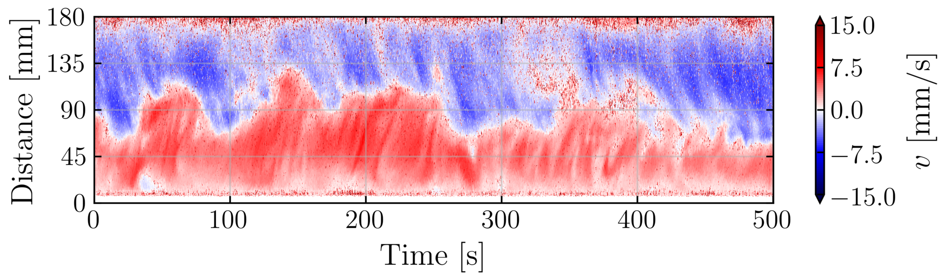
Figure 3: Contour-plot of Mid1 sensor data at 9 A and 25 Hz. The sampling time of this particular measurement was reduced to 75 ms. The unstable behaviour and the typical timescale of the flow changes are apparent.

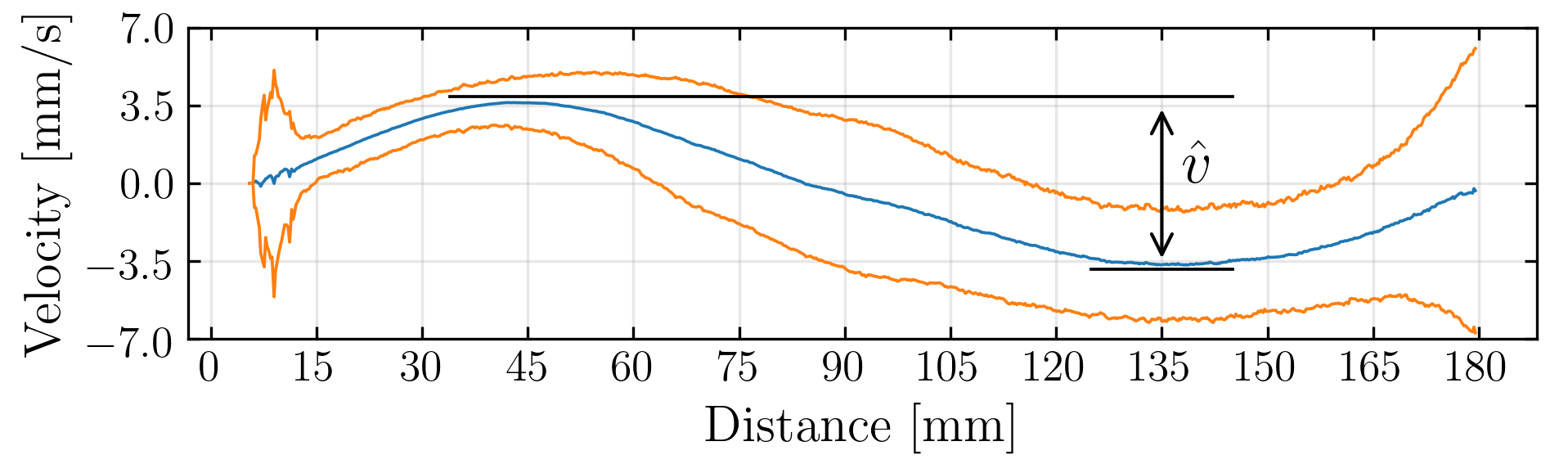
Figure 4: Time averaged velocity (blue) and standard deviation (orange) of the data of figure 3. The velocity value taken for comparison of parameters is the peak to peak amplitude of the averaged velocity $\hat{v}$.

III Numerical simulations

The corresponding numerical simulations of the tide-like liquid metal flow were performed using the open source code library OpenFOAM^© 5.x openfoam . The geometry of the entire model (Fig. 5) emulates as close as possible the real experiment, including all physical parameters. The flow in the cell was computed solving the incompressible Navier-Stokes equation

$$\frac{\partial\bm{u}}{\partial t}+(\bm{u}\cdot\nabla)\bm{u}=-\nabla p+\nu\nabla^{2}\bm{u}+\bm{f}_{EM}\,,$$ (1)

where the time-constant electromagnetic force density $\bm{f}_{EM}$ was pre-computed with Opera 1.7. Opera uses the FEA-Method to solve the Maxwell equations and to output the body force opera2018 . At all solid container walls the no-slip condition $u=0$ was chosen as boundary condition for the flow field. No turbulence model was used in the simulation of the fluid flow.

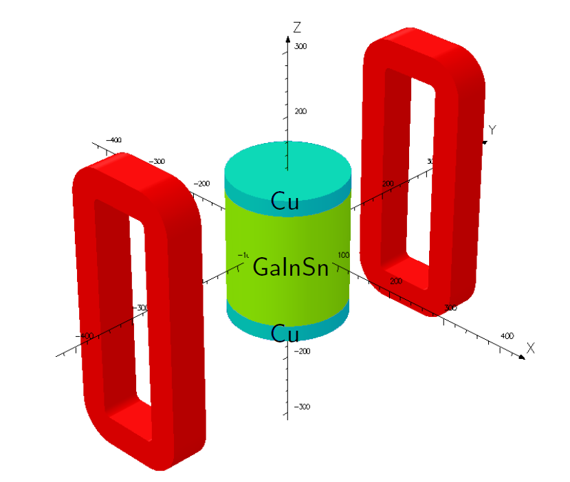
Figure 5: Model setup for pre-computing the electromagnetic force density in Opera 1.7. The two coils of the MultiMAG system which are used in our experiment are indicated in red.

Anticipating the typical Reynolds number of the generated tide-like flow, the cylindrical volume of 0.00458 m³ of the experimental cell was discretised using 1.3 million hexahedral cells. The smallest cell of the plane symmetric mesh has a volume of 0.373 mm³ and the biggest one 7.89 mm³ (see Fig. 6 for an impression). Close to the walls, the cells are contracted.

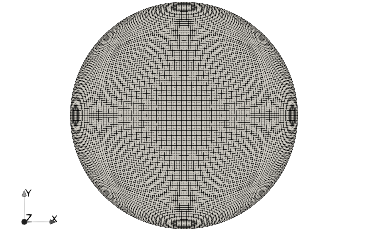
Figure 6: Symmetric hexahedral mesh with 1.3 million elements, cut in the central $x-y$ plane, as generated for the OpenFOAM simulations.

For the correct computation of the electromagnetic body force it is important to take into account the copper plates at the top and the bottom which tend to homogenize (in vertical direction) the body force in the fluid region. With increasing frequency this force is concentrated at the side walls, due to the skin effect. A typical force structure is shown (for the special case 9.7 A and 25 Hz) in Fig. 7. Evidently, the force mainly pushes radially inward along the $x$-axis, generating the two oppositely directed jets which were already visible in the experimental results (Fig. 3).

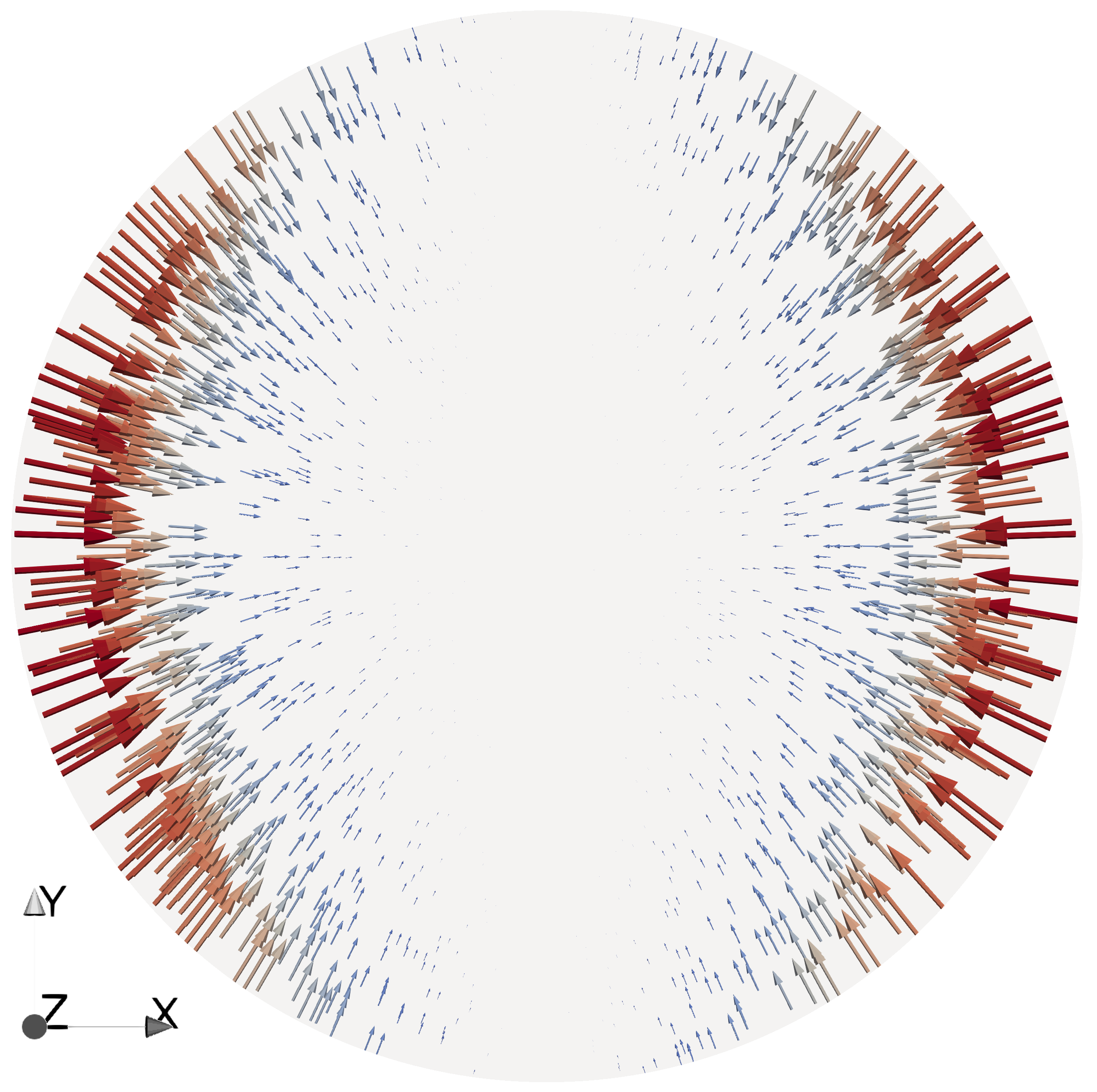
Figure 7: Structure of the body force as computed with Opera and imported into OpenFOAM. The force points mainly radially inward along the $x$-axis.

In the OpenFOAM simulation, at t = 0 s the body force is applied to a u = 0 m/s base state. After some time, the flow reaches a quasi-steady state. The specific flow structure, produced by an excitation current with 2.4 A and 25 Hz and averaged over a simulation time of 10000 s, is illustrated in Fig. 8. At all three selected heights, it shows the presence of four very similar, quasi-two-dimensional vortices, which are driven by the radially inward directed body force along the $x$-axis. Figure 9 depicts in more detail this vortex structure in the mid-height $x-y$-plane. While the time-averaged flow field shows a very regular structure, the instantaneous flow can significantly deviate from that average. This is illustrated in Fig. 10 in which the four-vortex structure is barely visible anymore.

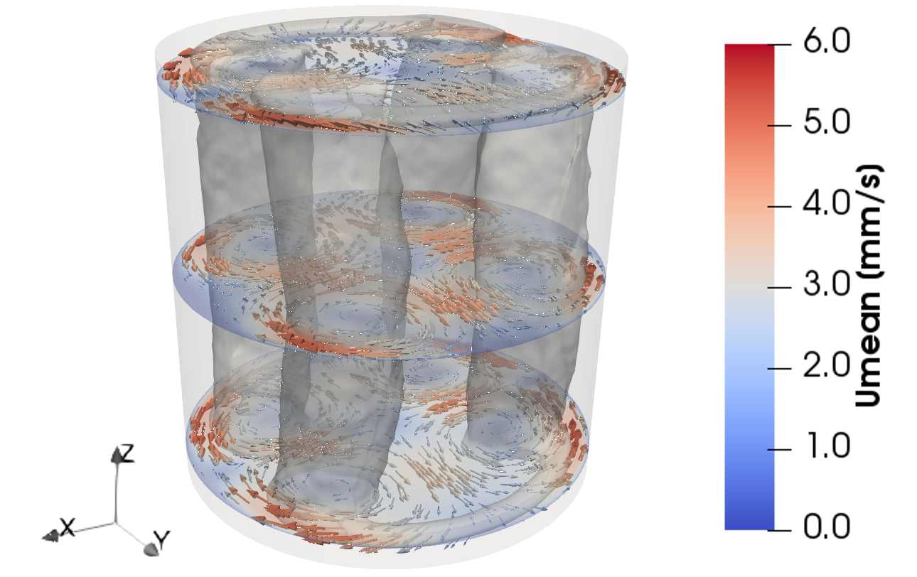
Figure 8: Velocity field time averaged over 10000 s, showing four quasi-two-dimensional vortices. I=9.8 A and f=25 Hz

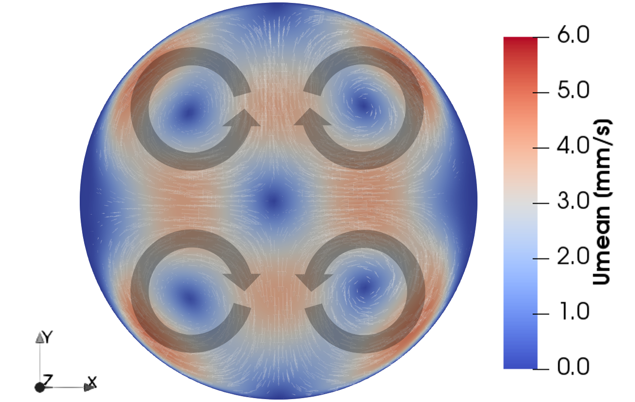
Figure 9: Velocity field time averaged over 10000 s, highlighting the four quasi-two-dimensional vortices at mid-height. I=9.8 A and f=25 Hz

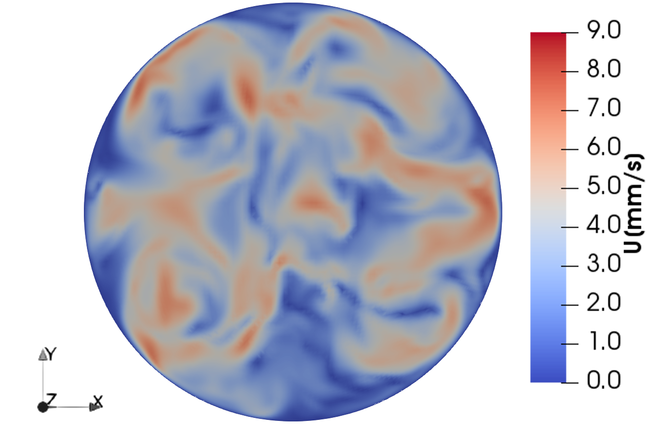
Figure 10: Instantaneous flow structure at mid-height and t=2760 s. I=9.8 A and f=25 Hz

IV Results

In this section we will present and compare the experimentally measured velocity fields with the numerically determined ones. In most detail we will discuss the results for the three current amplitudes 9.7 A, 5.9 A, 2.4 A, with frequency 25 Hz, while a few more results will be presented for currents up to 50 A and frequencies up to 200 Hz.

The parameter combination 9.7 A and 25 Hz produces relatively high flow velocities which can be clearly identified by UDV. For six selected sensors, Fig. 11 shows the contour plots of the actually measured signal (left column) and of corresponding “virtual sensors” as extracted from the numerical simulation (right column). Evidently, sensor “Mid3”, measuring along the $y$-axis at mid-height, shows a stable flow structure which points from the center towards the wall, leading to a negative projection (blue) close to the sensor, and a positive projection (red) at greater depth of the ultrasonic beam. While the division point between these two outward directed jets remains rather stable, there are some fluctuations both in the measured amplitudes and in the simulation.

In comparison with this quiet behaviour, sensor “Mid1” shows much stronger fluctuations. As mentioned above, these fluctuations are due to an instability of the stagnation point where the two inward directed jets converge toward each other. This leads to a bi-modal behaviour, with a tendency of the stagnation point to stay for most of the time at either side of the center rather than at the center itself.

The behaviour at the top and the bottom is not very different from that at mid-height, as exemplified here for the inward directed jets at the top (“Top1”) and the outward directed jets at the bottom (“Bot3”).

The most unstable situation is found at the sensors of position “2" with a 45 degree angle to the coils which are situated between sensors “1” and “3”. Evidently, at sensor “Top2” the flow projection onto the ultrasound beam fluctuates strongly and correlates thereby significantly with the movement of the stagnation point of “Top1”. “Top2” is also sensitive to azimuthal rotations of the flow structure about the cylinder axis. A similar fluctuation behaviour is seen in “Bot2”.

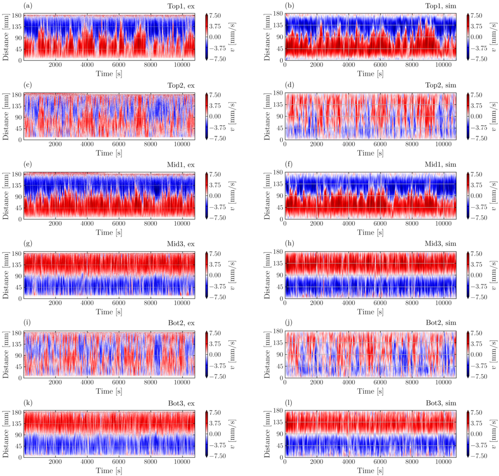
Figure 11: Contour plots of the flow speed for 9.7 A and 25 Hz. The left column shows measurement data, while the right column shows virtual sensor data from the simulations.

The corresponding contour plots for the lower current amplitudes 5.9 A and 2.45 A are presented in Fig. 12 and Fig. 13, respectively. Compared with the previous case of 9.7 A, both the flow amplitude and the typical frequency of the oscillation of the stagnation point decreases for the case with 5.9 A. For the extreme case with 2.45 A, we observe a very long transient behaviour for the onset of the fluctuations. The typical flow velocities are in the order of 1 mm/s which makes their clear identification by UDV challenging.

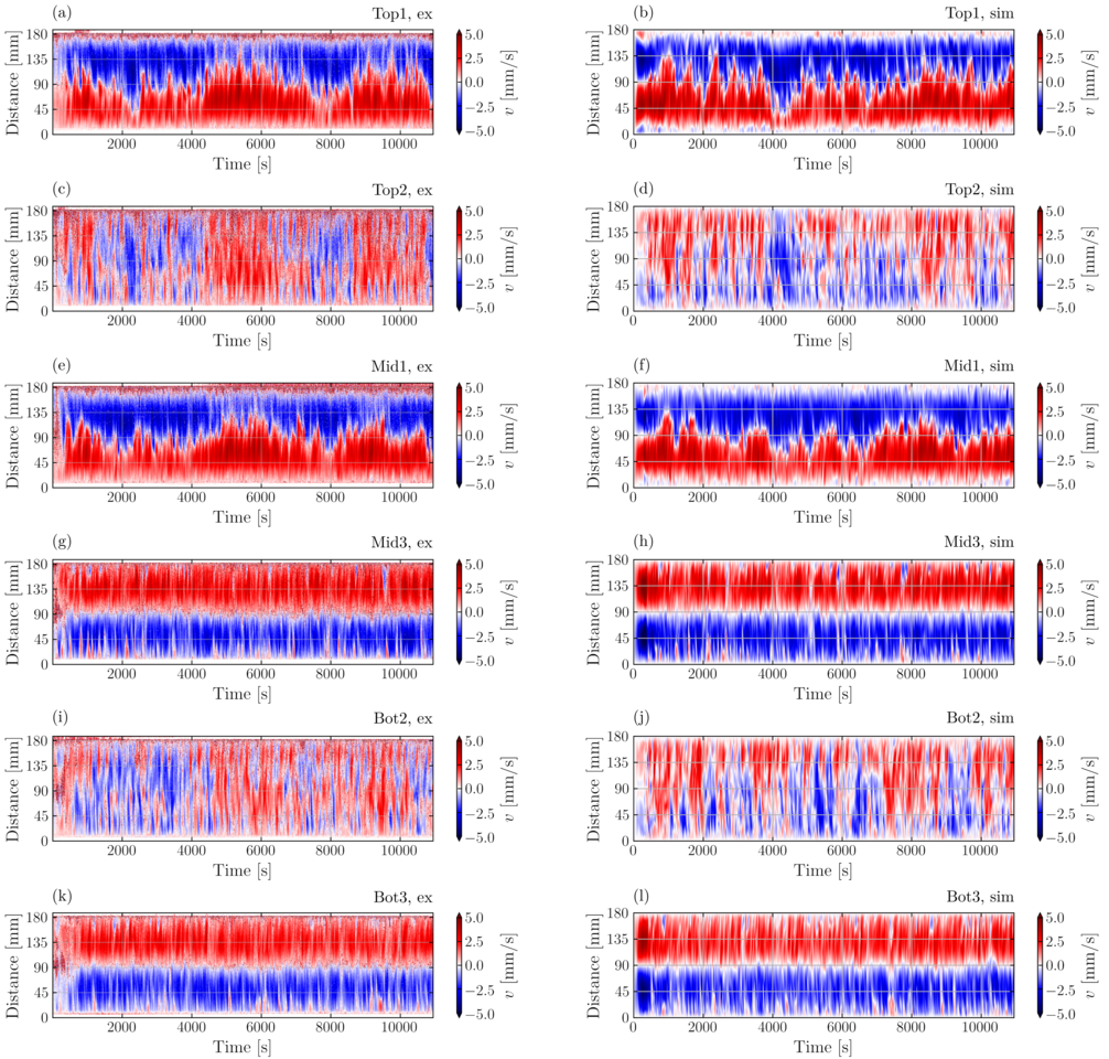
Figure 12: Contour plots of the flow speed for 5.9 A and 25 Hz. The left column shows measurement data, while the right column shows virtual sensor data from the simulations.

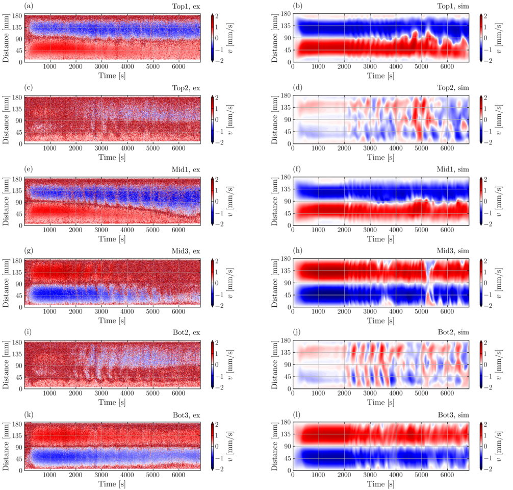
Figure 13: Contour plots of the flow speed for 2.45 A and 25 Hz. The left column shows measurement data, while the right column shows virtual sensor data from the simulations.

Apart from the mentioned oscillatory motion of the stagnation point, for the time-averaged flow structure we find a nearly perfect agreement between measurement and simulation. For the case with 9.7 A and 25 Hz, this is illustrated for sensors Mid1 and Mid3 in Fig. 14 and Fig. 15, respectively.

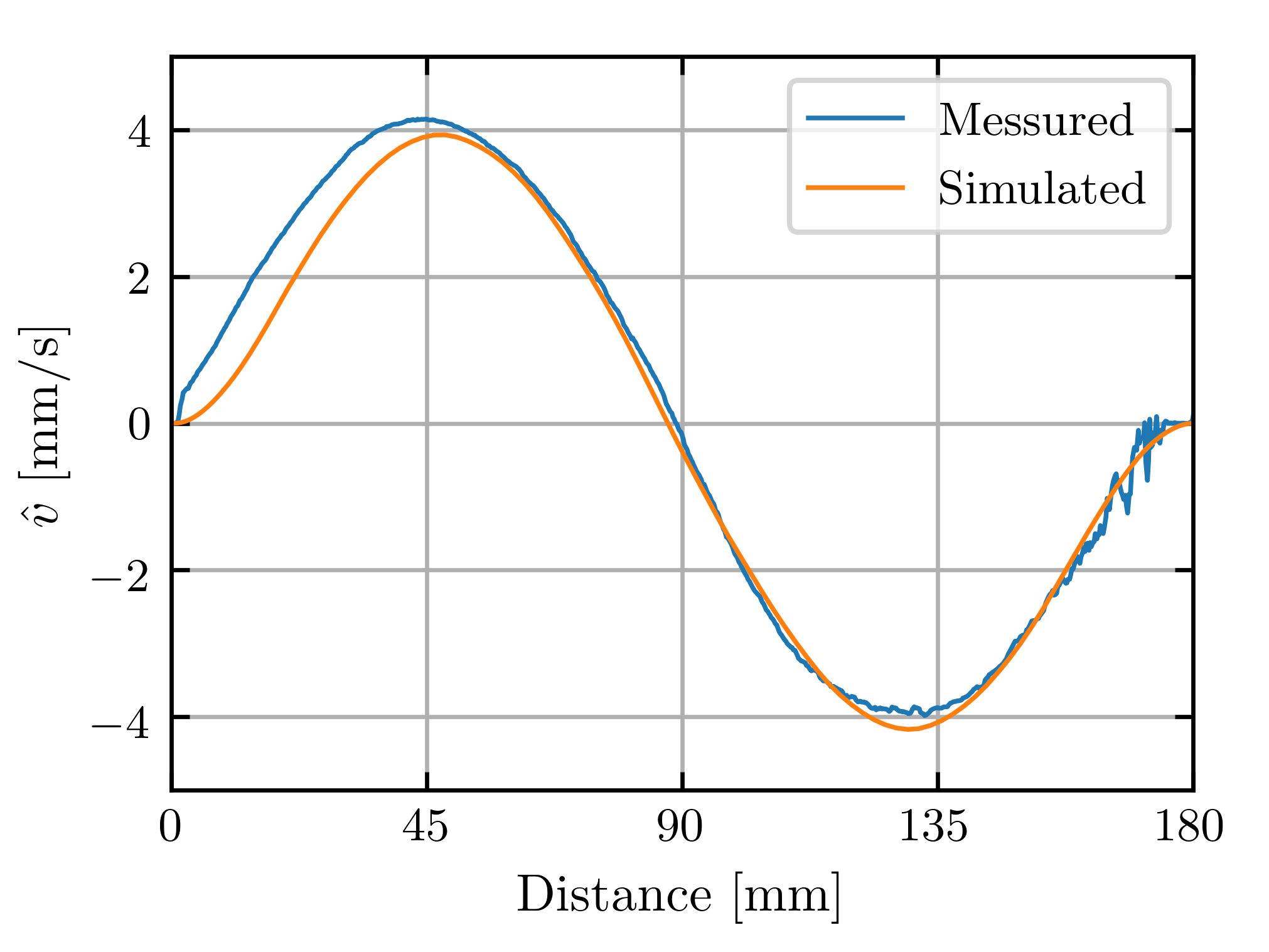
Figure 14: Comparison of simulated and measured average flow speed for sensor Mid1. I=9.8 A, f=25 Hz

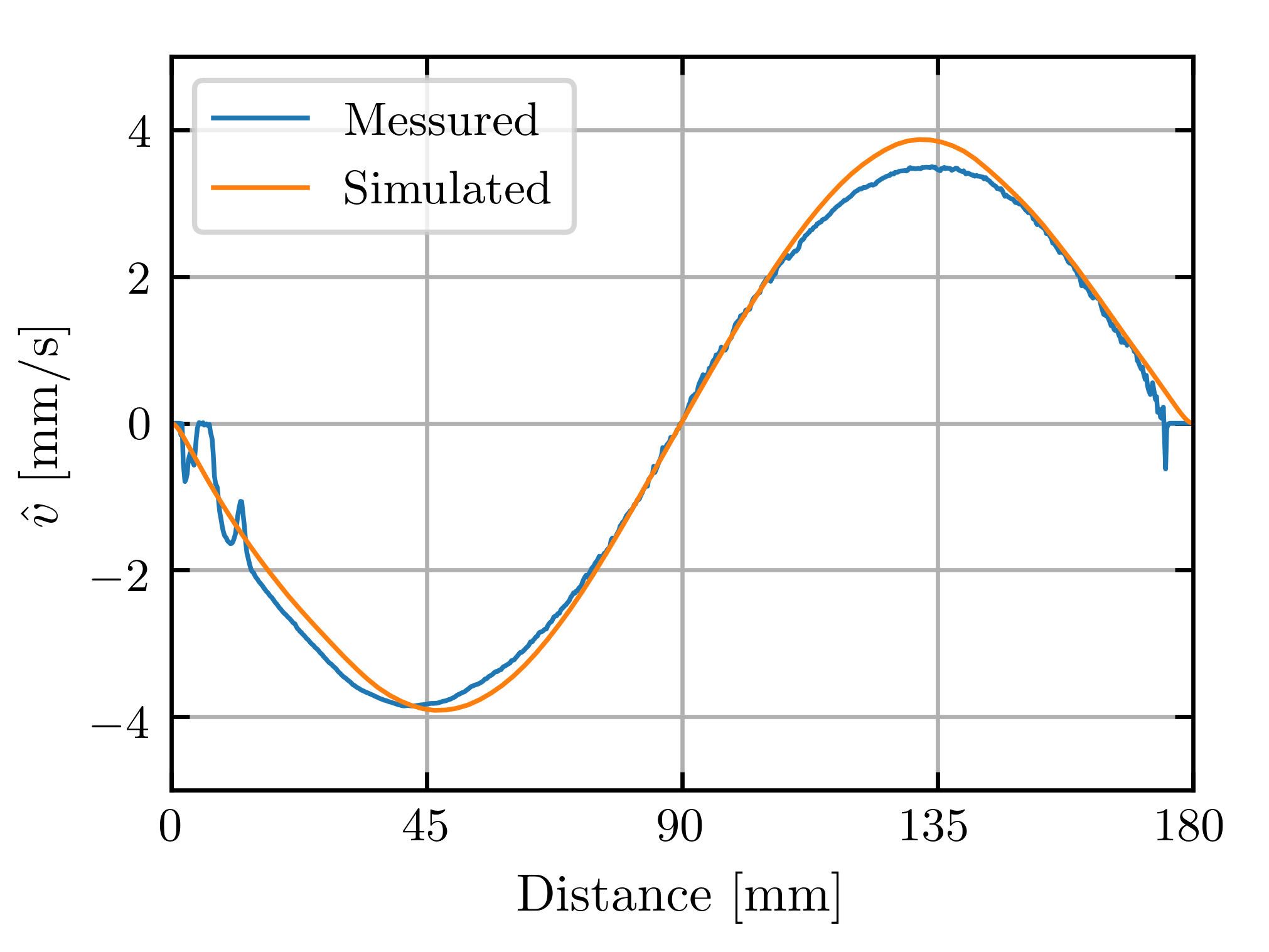
Figure 15: Comparison of simulated and measured average flow speed for sensor Mid3. I=9.8 A, f=25 Hz

The bi-modal behaviour of the stagnation point of the two inward directed jets is analysed in Fig. 16. It shows, for the three considered current amplitudes, the experimentally measured and numerically determined probability densities of the velocity in $x$-direction (as seen by sensor Mid1) in the centre of the cell. Apart from some slight quantitative differences, experiments and simulations show a distinct bi-modality of this velocity component. Due to the finite experimental/simulation time and possibly some geometric imperfections of the experiment, the bi-modality is not perfectly symmetric. For the lowest current 2.45 A the period of the stagnation point oscillation is already so large that the stagnation point stays completely on one side.

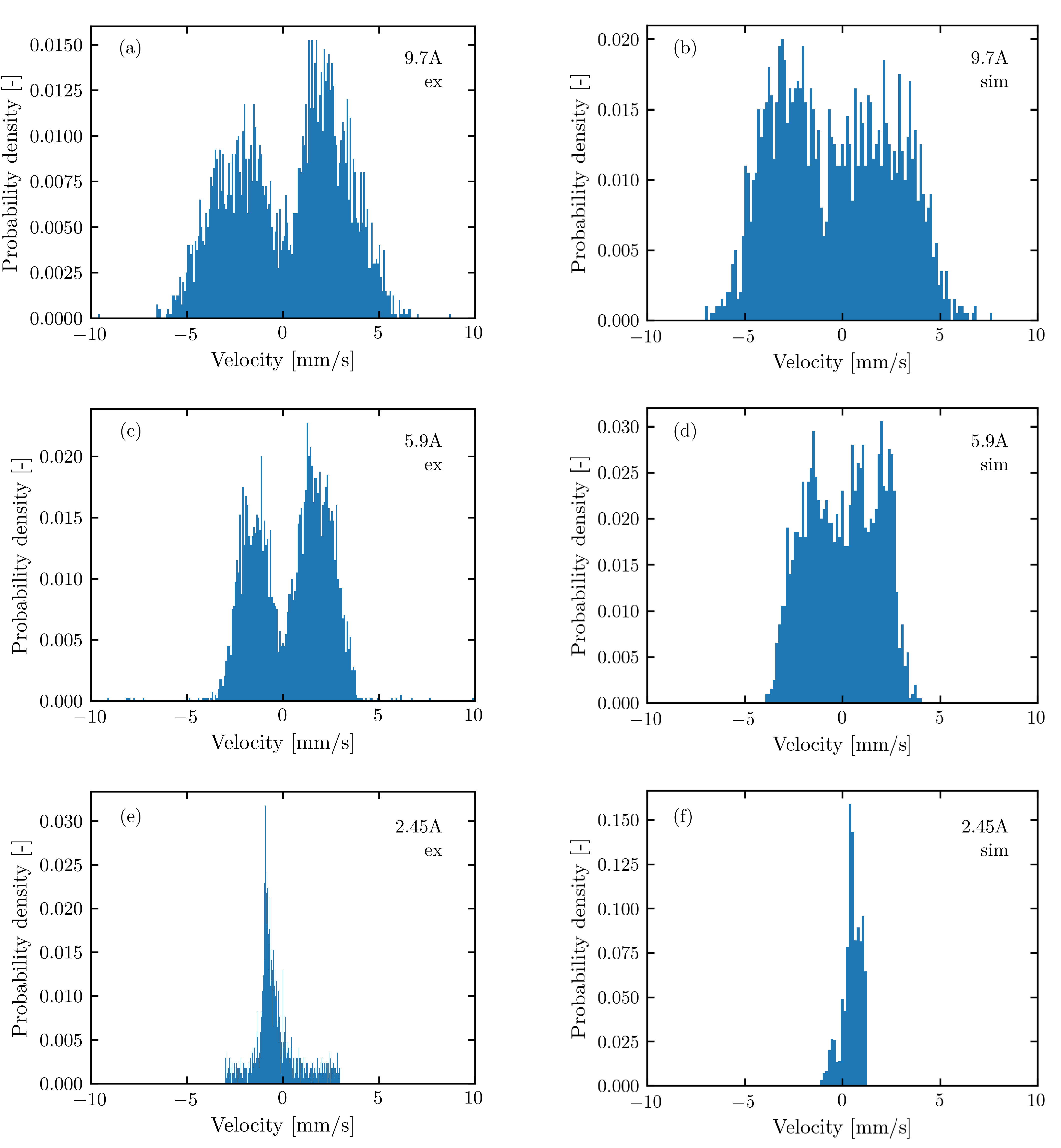
Figure 16: Histograms of the velocity of sensor Mid1 at the centre of the cylinder. On the left experimental data, on the right, CFD velocities.

After focusing on the flow behaviour for three particular, and weaker, current amplitudes, we will now summarize the dependence of the averaged flow amplitudes on the amplitude and the frequency of the current. For frequencies 25 Hz and 100 Hz, Fig. 17 indicates a mainly linear dependence of the flow amplitude on the current amplitude, with some notable deviations above 30 A. Corresponding simulations, carried out for 25 Hz until 30 A, show in general a good agreement with the experiments.

For two exemplary current amplitudes 19.4 A and 48.5 A, Fig. 18 illustrates the dependence of the flow amplitude on the frequency of the current. Here we observe a maximum approximately at 50-100 Hz, depending mildly on the current amplitude. At too low frequencies, the slowly changing magnetic field only weakly couples to the flow, while for too high frequencies the field is hindered in penetrating the vessel by the skin effect. The frequency 25 Hz seems particularly suitable for the later synchronization experiments since on the one hand, it is only slightly below the optimum frequency, and has on the other hand a large enough penetration depth to produce a rather smooth forcing distribution that is not too closely concentrated at the walls.

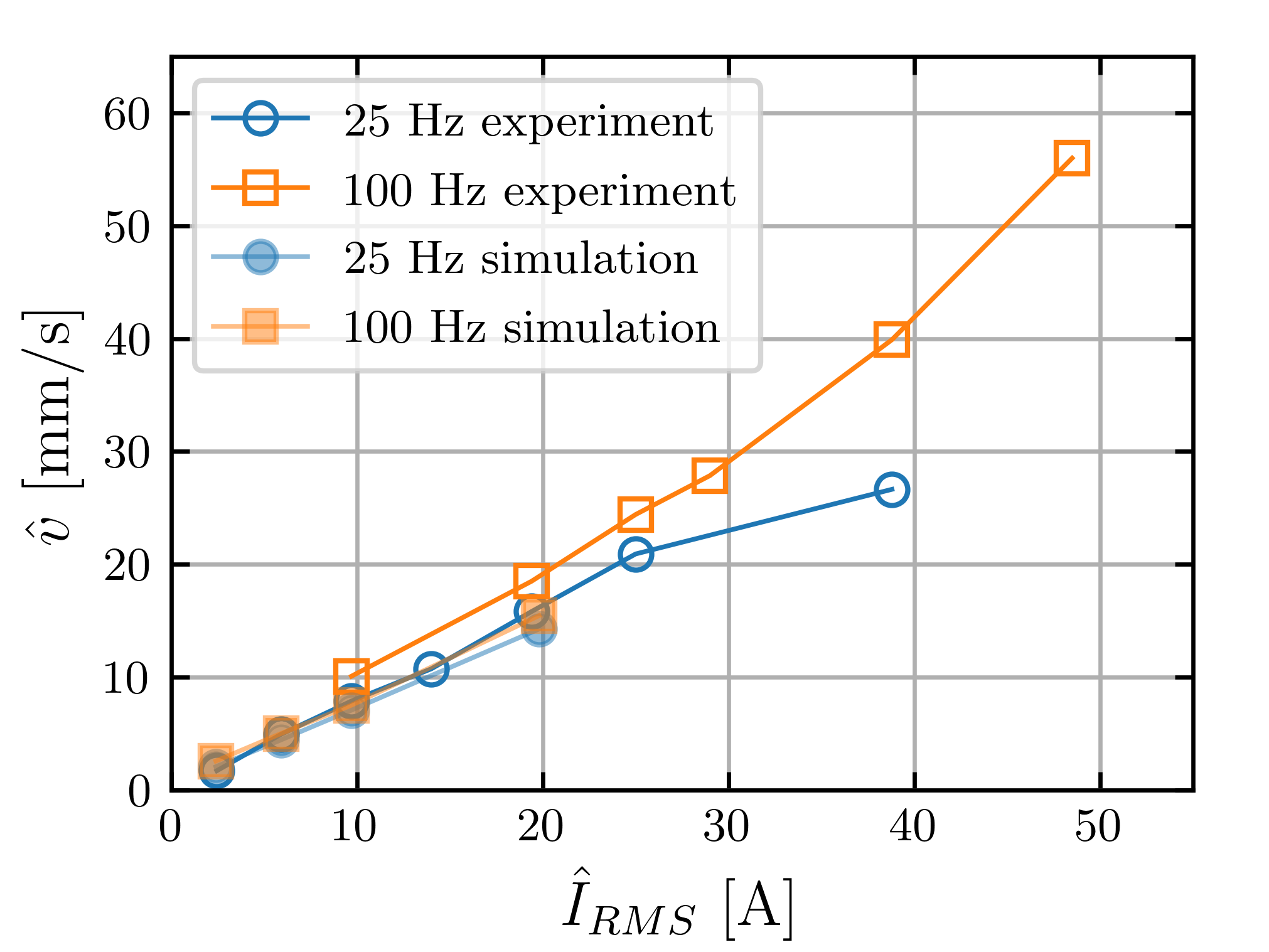
Figure 17: Current variation. X-axis: the root-mean-square of the alternating current in the RMF-coils. Y-axis: peak-to-peak velocity as described in Fig. 4. The curves differ by the frequency of the alternating current. The 2.45A experimental point is taken from a 30 minutes measurement, which is comparably short to the fluid motion time scale.

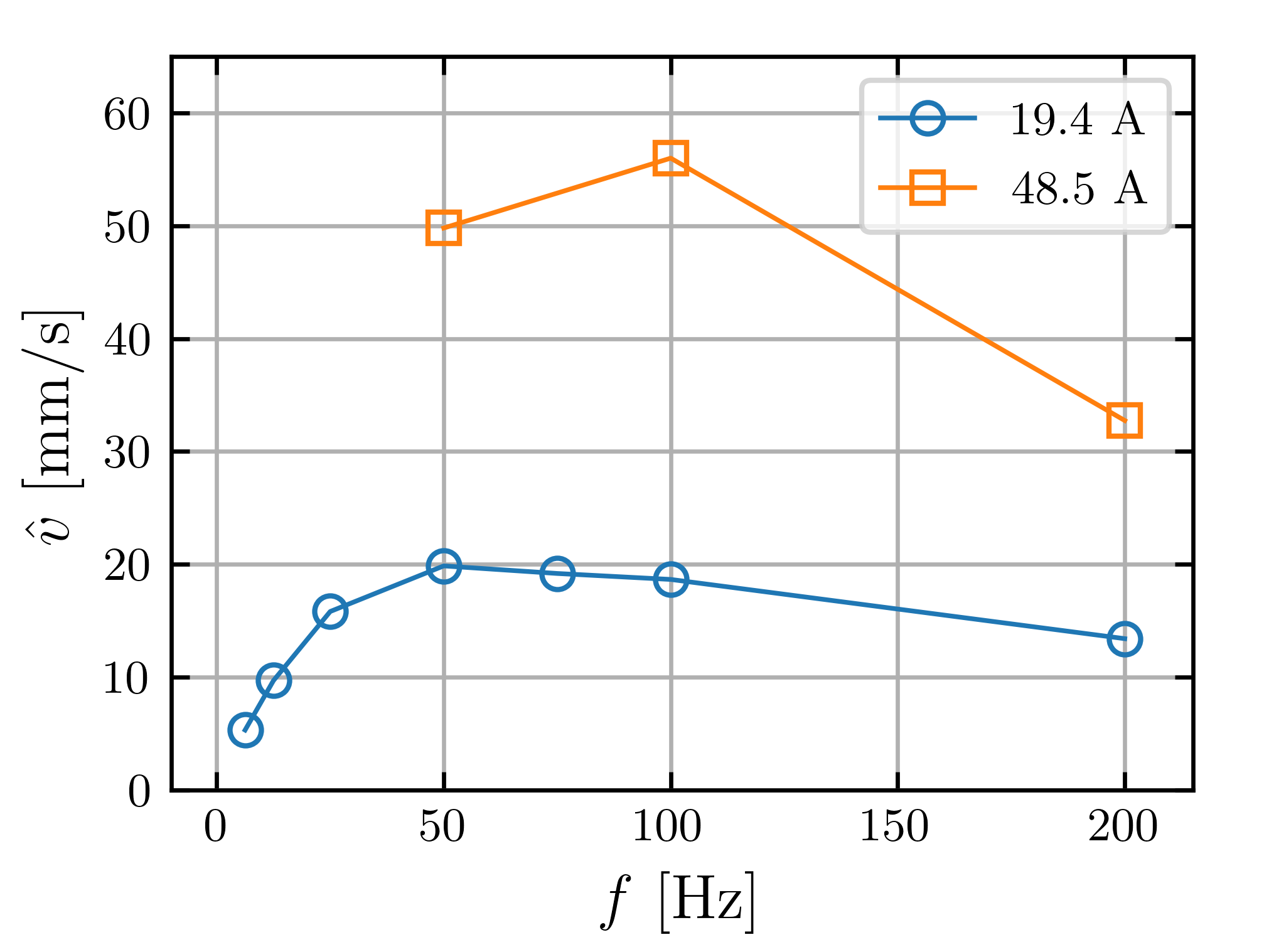
Figure 18: Frequency variation. X-axis: frequency of the alternating current in the RMF-coils. Y-axis: peak-to-peak velocity as described in Fig. 4. The curves are dependent on the current amplitude.

Our last result concerns the dependence of some typical time-scales on the current amplitude. While neither experiments nor simulations are long enough to allow for a reasonable statistics of the periods of the oscillation between different stagnation points, we can still determine the build-up time for the saturated mean square velocity $\bar{u^{2}}$, where typically the oscillation starts. The corresponding dependencies, obtained numerically and experimentally, are plotted in Fig. 19. As $\bar{u^{2}}$ is not available in the experiments, the points were estimated from the destabilization of the stagnation point in the contour plots.

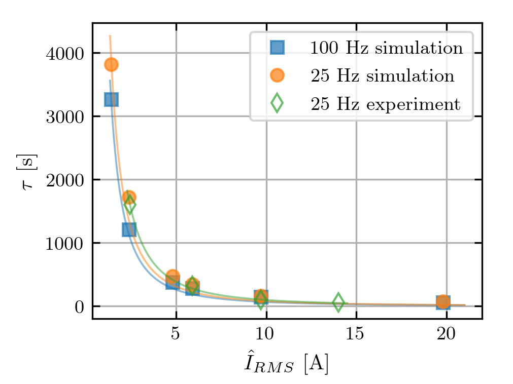
Figure 19: Time until the saturated value of $\bar{u^{2}}$ is reached. The experimental points are an estimate from the destabilization of the stagnation point in the Mid1 data. Fit parameters are listed in Table 1.

According to the Navier-Stokes equation and the induction equation, the acceleration of the fluid is proportional to the squared current amplitude. Therefore the build-up time $\tau_{b}$ is modelled to decrease with increasing current amplitude $\hat{I}_{RMS}$ following the equation

$$\tau_{b}=\frac{1}{a\cdot\hat{I}_{RMS}^{2}}$$ (2)

The determined fit parameters are listed in Table 1.

Table 1: Fit parameters “a” for Eq. 2 used in Fig. 19, with $r^{2}$ denoting the square of Pearsons correlation coefficient.

	a $[s^{-1}A^{-2}]$	$r^{2}$
25 Hz sim	1.286e-4	0.9812
25 Hz exp	1.037e-4	0.9987
100 Hz sim	1.541e-4	0.9956

At the lowest applied current of 2.45 A with a frequency of 25 Hz, the flow becomes unstable at $\tau_{b}\approx 1800\,\mathrm{s}$. With view on the later RBC experiment LSC-Till-2019 this exceeds the Large-Scale-Circulation (LSC) time by more than one order of magnitude. If we consider a sinusoidal swelling excitation of the tide-like forcing, the choice of I=2.45 A seems therefore not ideal. For this purpose, currents of 5.9 A with a build-up time $\tau_{b}\approx 300\,\mathrm{s}$, or I=9.7 A with $\tau_{b}\approx 150\,\mathrm{s}$, seem to be more suitable. However, as the $m=2$ forcing is supposed only to synchronize the sloshing instability of the LSC and not to dominate the entire flow structure in the vessel, for each Rayleigh number a optimization of the current will be required.

V Conclusions and prospects

In this paper we have compared experimental and numerical results on the tide-like flow in a cylindrical volume of a liquid metal that is driven by AC currents in two oppositely situated coils. With Ampere-turns in the order of 1000 A flow speeds of 10 mm/s are easily obtainable, despite the relatively large distance of the coils from the rim of the liquid metal. The dependence of the flow intensity on the AC current frequency shows a rather broad plateau between 25 and 100 Hz; at 25 Hz we find a good compromise between a not too shallow skin depth and a reasonable forcing.

In the next step we plan to act with the modulated electromagnetic forcing onto the typical LSC flow of RB convection. As shown in Zuerner2019 , the free fall time $\tau_{ff}$ of the LSC is in the range of a few seconds, leading to a typical oscillation frequency of the sloshing mode of $\tau_{osc}\sim 10\tau_{ff}$ of some tens of seconds. This also correspond to the the period of modulating the $m=2$ forcing which we expect will lead to a resonant excitation of the sloshing mode, and thereby of the helicity oscillation of the LSC.

References

- (1) N. Weber, V. Galindo, F. Stefani, and T. Weier, "The Tayler instability at low magnetic Prandtl numbers: between chiral symmetry breaking and helicity oscillations," New Journal of Physics, 17, 113013 (2015).
- (2) F. Stefani, A. Giesecke, N. Weber, and T. Weier, "Synchronized helicity oscillations: a link between planetary tides and the solar cycle?" Solar Phys. 291, 2197 (2016).
- (3) F. Stefani, A. Giesecke, and T. Weier, "On the synchronizability of Tayler-Spruit and Babcock-Leighton type dynamos," Sol. Phys. 293, 12 (2018).
- (4) F. Stefani, A. Giesecke, and T. Weier, "A model of a tidally synchronized solar dynamo," Sol. Phys. 294, 60 (2019).
- (5) F. Stefani, A. Giesecke, M. Seilmayer, R. Stepanov, and T. Weier, "Schwabe, Gleissberg, Suess-de Vries: Towards a consistent model of planetary synchronization of solar cycles," Magnetohydrodynamics, in press (2020); arXiv:1910.10383
- (6) R. J. Tayler, "The adiabatic stability of stars containing magnetic fields - I.Toroidal fields," Mon. Not. R. Astron. Soc. 161, 365–380 (1973).
- (7) M. Seilmayer, F. Stefani, T. Gundrum, T. Weier, G. Gerbeth, M. Gellert, and G. Rüdiger, "Experimental evidence for a transient Tayler instability in a cylindrical liquid-metal column," Phys. Rev. Lett. 108, 244501 (2012).
- (8) M. Dikpati, P.S. Cally, S.W. McInstosh, and E. Heifetz, "The origin of the "seasons" in space weather," Sci. Rep. 7, 14750 (2017).
- (9) S.W. McInstosh, W.J. Cramer, M. Pichardo Marcano, and R.J. Leamon, "The detection of Rossby-like waves on the Sun," Nature Astron. 11, 0086 (2017).
- (10) X. Márquez-Artavia, C.A. Jones, and S.M. Tobias, "Rotating magnetic shallow water waves and instabilities in a sphere," Geophys. Astrophys. Fluid Dyn. 111, 282 (2017).
- (11) T. Zaqarashvili, "Equatorial magnetohydrodynamic shallow water waves in the solar tachocline," Astron Astrophys. 856, 32 (2018).
- (12) R. Krishnamurti, and L.N. Howard, "Large-scale flow generation in turbulent convection," Proc. Natl. Acad. Sci. 78, 1991 (1981).
- (13) M. Sano, X.-Z. Wu, and A. Libchaber, "Turbulence in helium-gas free convection," Phys. Rev. A 40, 6421 (1989).
- (14) T. Takeshita, T. Segawa, J.A. Glazier, and M. Sano, "Thermal turbulence in mercury," Phys. Rev. Lett. 76, 1465 (1996).
- (15) S. Cioni, S. Ciliberto, and J. Sommeria, "Strongly turbulent Rayleigh-Bénard convection in mercury: comparison with results at moderate Prandtl number," J. Fluid Mech. 335, 111 (1997).
- (16) H.-D. Xi, S. Lam., and K.-Q. Xia, "From laminar plumes to organized flows: the onset of large-scale circulation in turbulent thermal convection," J. Fluid Mech. 503, 47 (2004).
- (17) E. Brown and G. Ahlers, "Rotations and cessations of the large-scale circulation in turbulent Rayleigh-Bénard convection," J. Fluid Mech. 568, 351 (2006).
- (18) C. Resagk, R. du Puits, A. Thess, F.V. Dolzhansky, S. Grossman, F.F. Araujo, and D. Lohse, "Oscillations of the large scale wind in turbulent thermal convection," Phys. Fluids 18, 095105 (2006).
- (19) H.-D. Xi, and K.-Q. Xia, "Cessations and reversals of the large-scale circulation in turbulent thermal convection," Phys. Rev. E 75, 066307 (2008).
- (20) L.P. Kadanoff, "Turbulent heat flow: structure and scaling," Phys. Today 54, 34 (2001).
- (21) D. Funfschilling and G. Ahlers, "Plume motion and large scale circulation in a cylindrical Rayleigh-Bénard cell," Phys. Rev. Lett. 92, 194502 (2004).
- (22) H.-D. Xi, S.-Q. Zhou, T.-S. Chan, and K.-Q. Xia, "Origin of temperature oscillation in turbulent thermal convection," Phys. Rev. Lett. 102, 044503 (2009).
- (23) E. Brown, G. Ahlers, "The origin of oscillations of the large-scale circulation of turbulent Rayleigh-Bénard convection," J. Fluid Mech. 638, 383 (2009).
- (24) R. Khalilov, I. Kolesnichenko, A. Pavlinov, A. Mamykin, and A. Shestakov, "Thermal convection of liquid sodium in inclined cylinders," Phys. Rev. Fluids 3, 043503 (2018).
- (25) T. Wondrak, J. Pal, F. Stefani, V. Galindo, and S. Eckert, "Visualization of the global flow structure in a modified Rayleigh-B énard setup using contactless inductive flow tomography," Flow. Meas. Instrum. 62, 269 (2018).
- (26) T. Zürner, F. Schindler, T. Vogt, S. Eckert, and J. Schumacher, "Coherent large-scale flow in turbulent liquid metal convection,", J. Fluid Mech., submitted (2019)
- (27) C. Morize, M. Le Bars, P. Le Gal, and A. Tilgner, "Experimental determination of zonal winds driven by tides,", Phys. Rev. Lett. 104. 214501 (2010)
- (28) J. Pal, A. Cramer, T. Gundrum, and G. Gerbeth, "MULTIMAG - A MUL- TIpurpose MAGnetic system for physical modelling in magnetohydrodynamics," Flow Meas. Instr. 20, 241 (2009).
- (29) R. Stepanov, F. Stefani, "Electromagnetic forcing of a flow with the azimuthal wave number m = 2 in cylindrical geometry", Magnetohydrodynamics 55, No. 1/2, 207-214 (2019).
- (30) Y. Plevachuk, V. Sklyarchuk, N. Shevchenko, and S. Eckert, "Electrophysical and structure-sensitive properties of liquid Ga-In alloys," Int. J. Mater. Res. 106, 66 (2015).
- (31) T. Zürner, F. Schindler, T. Vogt, S. Eckert, J. Schumacher, "Combined measurement of velocity and temperature in liquid metal convection," J. Fluid Mech. 876, 1108-1128 (2019)
- (32) OpenCFD, OpenFOAM - The Open Source CFD Toolbox - User’s Guide, OpenCFD Ltd., United Kingdom, 3rd ed. (2015).
- (33) Opera, Opera - Simulation Software (Brochure), ©Dassault Systèms, (2018)