ABSTRACT

The search for flavour-changing neutral current effects in $B$-meson decays is a powerful probe of physics beyond the Standard Model. Deviations from SM behaviour are often quantified by extracting the preferred values of the Wilson coefficients of an operator product expansion. We use the FlavBit module of the GAMBIT package to perform a simultaneous global fit of the Wilson coefficients $C_{7}$, $C_{9}$, and $C_{10}$ using a combination of all current data on $\mathit{{b}{}_{\mspace{-3.0mu}\scriptstyle{}}^{\mspace{-1.0mu}\scriptstyle{}}}\to\mathit{{s}{}_{\mspace{-3.0mu}\scriptstyle{}}^{\mspace{-1.0mu}\scriptstyle{}}}\mathit{{\mu}{}_{\mspace{-3.0mu}\scriptstyle{}}^{\mspace{-1.0mu}\scriptstyle{+}}}\mathit{{\mu}{}_{\mspace{-3.0mu}\scriptstyle{}}^{\mspace{-1.0mu}\scriptstyle{-}}}$ transitions. We further extend previous analyses by accounting for the correlated theoretical uncertainties at each point in the Wilson coefficient parameter space, rather than deriving the uncertainties from a Standard Model calculation. We find that the best fit deviates from the SM value with a significance of 6.6$\sigma$. The largest deviation is associated with a vector coupling of muons to $b$ and $s$ quarks.

1 Introduction

In the Standard Model (SM), flavour-changing neutral currents (FCNC) are heavily suppressed by the Glashow-Iliopoulos-Maiani (GIM; PhysRevD.2.1285 ) mechanism. Since the start of the LHC, experiments have observed numerous deviations from the predictions of the SM in $\mathit{{b}{}_{\mspace{-3.0mu}\scriptstyle{}}^{\mspace{-1.0mu}\scriptstyle{}}}\to\mathit{{s}{}_{\mspace{-3.0mu}\scriptstyle{}}^{\mspace{-1.0mu}\scriptstyle{}}}\mathit{{\mu}{}_{\mspace{-3.0mu}\scriptstyle{}}^{\mspace{-1.0mu}\scriptstyle{+}}}\mathit{{\mu}{}_{\mspace{-3.0mu}\scriptstyle{}}^{\mspace{-1.0mu}\scriptstyle{-}}}$ transitions, starting with the 2013 LHCb collaboration observation of a deviation in the $P^{\prime}_{5}$ observable in the range $q^{2}\in\left[4.30,8.68\right]~{}\rm GeV^{2}/c^{4}$ of the decay $\mathit{{B}{}_{\mspace{-3.0mu}\scriptstyle{d}}^{\mspace{-1.0mu}\scriptstyle{}}}\to\mathit{{K}{}_{\mspace{-3.0mu}\scriptstyle{}}^{\mspace{-1.0mu}\scriptstyle{*0}}}\mathit{{\mu}{}_{\mspace{-3.0mu}\scriptstyle{}}^{\mspace{-1.0mu}\scriptstyle{+}}}\mathit{{\mu}{}_{\mspace{-3.0mu}\scriptstyle{}}^{\mspace{-1.0mu}\scriptstyle{-}}}$ Aaij:2013qta . Further discrepancies were later observed in measurements of the $\mathit{{B}{}_{\mspace{-3.0mu}\scriptstyle{s}}^{\mspace{-1.0mu}\scriptstyle{}}}\to\mathit{{\phi}{}_{\mspace{-3.0mu}\scriptstyle{}}^{\mspace{-1.0mu}\scriptstyle{}}}\mathit{{\mu}{}_{\mspace{-3.0mu}\scriptstyle{}}^{\mspace{-1.0mu}\scriptstyle{+}}}\mathit{{\mu}{}_{\mspace{-3.0mu}\scriptstyle{}}^{\mspace{-1.0mu}\scriptstyle{-}}}$ Aaij:2013aln ; LHCb:2021zwz , $\mathit{{B}{}_{\mspace{-3.0mu}\scriptstyle{}}^{\mspace{-1.0mu}\scriptstyle{}}}\to\mathit{{K}{}_{\mspace{-3.0mu}\scriptstyle{}}^{\mspace{-1.0mu}\scriptstyle{}}}\mathit{{\mu}{}_{\mspace{-3.0mu}\scriptstyle{}}^{\mspace{-1.0mu}\scriptstyle{+}}}\mathit{{\mu}{}_{\mspace{-3.0mu}\scriptstyle{}}^{\mspace{-1.0mu}\scriptstyle{-}}}$ Aaij:2016cbx , and $\mathit{{\Lambda}{}_{\mspace{-3.0mu}\scriptstyle{b}}^{\mspace{-1.0mu}\scriptstyle{}}}\to\mathit{{\Lambda}{}_{\mspace{-3.0mu}\scriptstyle{}}^{\mspace{-1.0mu}\scriptstyle{}}}\mathit{{\mu}{}_{\mspace{-3.0mu}\scriptstyle{}}^{\mspace{-1.0mu}\scriptstyle{+}}}\mathit{{\mu}{}_{\mspace{-3.0mu}\scriptstyle{}}^{\mspace{-1.0mu}\scriptstyle{-}}}$ Aaij:2015xza decays in both the angular and branching fraction observables. Given the consistency of the observations, other experiments Abdesselam:2016llu ; Aaboud:2018krd ; Sirunyan:2017dhj have performed measurements of the $\mathit{{B}{}_{\mspace{-3.0mu}\scriptstyle{d}}^{\mspace{-1.0mu}\scriptstyle{}}}\to\mathit{{K}{}_{\mspace{-3.0mu}\scriptstyle{}}^{\mspace{-1.0mu}\scriptstyle{*0}}}\mathit{{\mu}{}_{\mspace{-3.0mu}\scriptstyle{}}^{\mspace{-1.0mu}\scriptstyle{+}}}\mathit{{\mu}{}_{\mspace{-3.0mu}\scriptstyle{}}^{\mspace{-1.0mu}\scriptstyle{-}}}$ decay, finding results consistent with the discrepancies seen earlier.

As has been studied in previous analyses, the discrepancies can be solved by reducing the $C_{9}$ Wilson coefficient by one quarter of the SM value (see for example Refs. DAmico:2017mtc ; Geng:2017svp ; Hurth:2017hxg ; Alguero:2019ptt ; Alok:2019ufo ; Ciuchini:2019usw ; Aebischer:2019mlg ; Kowalska:2019ley ; Arbey:2018ics ; Datta:2019zca ; Arbey:2019duh ). Unfortunately, these processes suffer from non-factorisable corrections, making the size of the theoretical uncertainties, and therefore the overall significance of the results, difficult to quantify (see Refs. Khodjamirian:2010vf ; Khodjamirian:2012rm ; Dimou:2012un ; Lyon:2013gba ; Lyon:2014hpa ; Bobeth:2017vxj ; Blake:2017fyh , and Hurth:2020rzx for a recent discussion of the hadronic corrections).

The SM predicts that the rate of $\mathit{{b}{}_{\mspace{-3.0mu}\scriptstyle{}}^{\mspace{-1.0mu}\scriptstyle{}}}\to\mathit{{s}{}_{\mspace{-3.0mu}\scriptstyle{}}^{\mspace{-1.0mu}\scriptstyle{}}}\mathit{{\mkern 4.0mu\overline{\mkern-4.0mu{\ell}}}{}_{\mspace{-2.0mu}\scriptstyle{}}^{\mspace{0.0mu}\scriptstyle{}}}\mathit{{\ell}{}_{\mspace{-3.0mu}\scriptstyle{}}^{\mspace{-1.0mu}\scriptstyle{}}}$ transitions is independent of the flavour of the leptons involved, except for mass effects which are negligible when studying the first two generations $\mathit{{\ell}{}_{\mspace{-3.0mu}\scriptstyle{}}^{\mspace{-1.0mu}\scriptstyle{}}}=\mathit{{e}{}_{\mspace{-3.0mu}\scriptstyle{}}^{\mspace{-1.0mu}\scriptstyle{}}},\mathit{{\mu}{}_{\mspace{-3.0mu}\scriptstyle{}}^{\mspace{-1.0mu}\scriptstyle{}}}$. In addition to the discrepancies seen purely with muons, the LHCb collaboration has therefore also performed explicit tests of lepton universality in $\mathit{{b}{}_{\mspace{-3.0mu}\scriptstyle{}}^{\mspace{-1.0mu}\scriptstyle{}}}\to\mathit{{s}{}_{\mspace{-3.0mu}\scriptstyle{}}^{\mspace{-1.0mu}\scriptstyle{}}}\mathit{{\mkern 4.0mu\overline{\mkern-4.0mu{\ell}}}{}_{\mspace{-2.0mu}\scriptstyle{}}^{\mspace{0.0mu}\scriptstyle{}}}\mathit{{\ell}{}_{\mspace{-3.0mu}\scriptstyle{}}^{\mspace{-1.0mu}\scriptstyle{}}}$ transitions. The first test is to measure the ratio $R_{\mathit{{K}{}_{\mspace{-3.0mu}\scriptstyle{}}^{\mspace{-1.0mu}\scriptstyle{}}}}\equiv\mathcal{B}(\mathit{{B}{}_{\mspace{-3.0mu}\scriptstyle{}}^{\mspace{-1.0mu}\scriptstyle{}}}\to\mathit{{K}{}_{\mspace{-3.0mu}\scriptstyle{}}^{\mspace{-1.0mu}\scriptstyle{}}}\mathit{{\mu}{}_{\mspace{-3.0mu}\scriptstyle{}}^{\mspace{-1.0mu}\scriptstyle{+}}}\mathit{{\mu}{}_{\mspace{-3.0mu}\scriptstyle{}}^{\mspace{-1.0mu}\scriptstyle{-}}})/\mathcal{B}(\mathit{{B}{}_{\mspace{-3.0mu}\scriptstyle{}}^{\mspace{-1.0mu}\scriptstyle{}}}\to\mathit{{K}{}_{\mspace{-3.0mu}\scriptstyle{}}^{\mspace{-1.0mu}\scriptstyle{}}}\mathit{{e}{}_{\mspace{-3.0mu}\scriptstyle{}}^{\mspace{-1.0mu}\scriptstyle{+}}}\mathit{{e}{}_{\mspace{-3.0mu}\scriptstyle{}}^{\mspace{-1.0mu}\scriptstyle{-}}})$, whilst a second is to measure $R_{\mathit{{K}{}_{\mspace{-3.0mu}\scriptstyle{}}^{\mspace{-1.0mu}\scriptstyle{\ast}}}}=\mathcal{B}(\mathit{{B}{}_{\mspace{-3.0mu}\scriptstyle{d}}^{\mspace{-1.0mu}\scriptstyle{}}}\to\mathit{{K}{}_{\mspace{-3.0mu}\scriptstyle{}}^{\mspace{-1.0mu}\scriptstyle{*0}}}\mathit{{\mu}{}_{\mspace{-3.0mu}\scriptstyle{}}^{\mspace{-1.0mu}\scriptstyle{+}}}\mathit{{\mu}{}_{\mspace{-3.0mu}\scriptstyle{}}^{\mspace{-1.0mu}\scriptstyle{-}}})/\mathcal{B}(\mathit{{B}{}_{\mspace{-3.0mu}\scriptstyle{d}}^{\mspace{-1.0mu}\scriptstyle{}}}\to\mathit{{K}{}_{\mspace{-3.0mu}\scriptstyle{}}^{\mspace{-1.0mu}\scriptstyle{*0}}}\mathit{{e}{}_{\mspace{-3.0mu}\scriptstyle{}}^{\mspace{-1.0mu}\scriptstyle{+}}}\mathit{{e}{}_{\mspace{-3.0mu}\scriptstyle{}}^{\mspace{-1.0mu}\scriptstyle{-}}})$. In both cases the SM prediction is known at the $1\%$ level, as the hadronic uncertainties cancel in taking the ratio of the two branching ratios. The LHCb experiment measured a lower value than the SM prediction with a significance of $3.1\sigma$ and $2.1-2.5\sigma$ for $R_{\mathit{{K}{}_{\mspace{-3.0mu}\scriptstyle{}}^{\mspace{-1.0mu}\scriptstyle{}}}}$ and $R_{\mathit{{K}{}_{\mspace{-3.0mu}\scriptstyle{}}^{\mspace{-1.0mu}\scriptstyle{\ast}}}}$ respectively LHCb:2021trn ; Aaij:2017vbb .

In this paper, we focus mainly on tests with muons, exploring the extent to which the combination of all such data to date either constrain flavour-universal new physics (i.e. coupling identically to all leptons) in $\mathit{{b}{}_{\mspace{-3.0mu}\scriptstyle{}}^{\mspace{-1.0mu}\scriptstyle{}}}\to\mathit{{s}{}_{\mspace{-3.0mu}\scriptstyle{}}^{\mspace{-1.0mu}\scriptstyle{}}}$ transitions, or prefer it in comparison to the SM. Using the FlavBit flavbit module of the Global and Modular Beyond-Standard Model Inference Tool (GAMBIT; gambit ; grev ), we carry out a model-independent analysis by simultaneously fitting three Wilson coefficients in an effective field theory for interactions of $b$ and $s$ quarks with leptons and photons. We significantly improve on previous analyses by explicitly re-computing theory uncertainties at every Wilson coefficient combination, rather than assuming that they are constant and given by their SM values across the entire parameter space. The final result is a 6.6$\sigma$ preference for new physics, overwhelmingly associated with the vector coupling of muons to $b$ and $s$ quarks.

We begin in Sec. 2 with a description of the effective field theory framework in which we work, followed by explanations of the observables (Sec. 3) and likelihoods (Sec. 4) involved in our fits. We show the results of our analysis in Sec. 5, including preferred regions of the Wilson coefficient parameter space and the spectrum of observables at our best-fit point, before concluding in Sec. 6.

2 Theoretical Framework

Our analysis is based on the effective Hamiltonian approach, in which the Operator Product Expansion is used to separate physics at low energies from a (possibly unknown) high energy theory. In this framework, the transition from an initial state $i$ to a final state $f$ is proportional to the squared matrix element $|\langle f|{\cal H}_{\rm eff}|i\rangle|^{2}$, with the effective Hamiltonian for $b\rightarrow s$ transitions given by

$$\mathcal{H}_{\rm eff}=-\frac{4G_{F}}{\sqrt{2}}V_{tb}V_{ts}^{*}\sum_{i=1}^{10}\Bigl{(}C_{i}(\mu)\mathcal{O}_{i}(\mu)+C^{\prime}_{i}(\mu)\mathcal{O}^{\prime}_{i}(\mu)\Bigr{)}\;.$$ (1)

$G_{F}$, $V_{tb}$ and $V_{ts}$ are SM parameters (the Fermi constant and two CKM matrix elements, respectively), $\mu$ is the energy scale at which the calculation is being performed, and the $O_{i}$ are local operators providing low-energy descriptions of high-energy physics that has been integrated out. The operators each come with an associated Wilson coefficient $C_{i}$ which, for a particular high-energy physics model, is calculable within the framework of perturbation theory. This is done by matching the high-scale theory to the low-energy effective theory at a scale $\mu_{W}$, which is of the order of the $W$ boson mass. The renormalisation group equations of the low-energy effective theory can then be used to evolve the Wilson coefficients to the scale $\mu_{b}$, which characterises $B$ meson decay calculations and is thus of order $m_{b}$.

The operators that are most relevant for rare B decays featuring FCNCs are

$$\mathcal{O}_{1} =(\bar{s}\gamma_{\mu}T^{a}P_{L}c)(\bar{c}\gamma^{\mu}T^{a}P_{L}b)\;,$$

$$\mathcal{O}_{2} =(\bar{s}\gamma_{\mu}P_{L}c)(\bar{c}\gamma^{\mu}P_{L}b)\;,$$

$$\mathcal{O}_{3} =(\bar{s}\gamma_{\mu}P_{L}b)\sum_{q}(\bar{q}\gamma^{\mu}q)\;,$$

$$\mathcal{O}_{4} =(\bar{s}\gamma_{\mu}T^{a}P_{L}b)\sum_{q}(\bar{q}\gamma^{\mu}T^{a}q)\;,$$

$$\mathcal{O}_{5} =(\bar{s}\gamma_{\mu_{1}}\gamma_{\mu_{2}}\gamma_{\mu_{3}}P_{L}b)\sum_{q}(\bar{q}\gamma^{\mu_{1}}\gamma^{\mu_{2}}\gamma^{\mu_{3}}q)\;,$$

$$\mathcal{O}_{6} =(\bar{s}\gamma_{\mu_{1}}\gamma_{\mu_{2}}\gamma_{\mu_{3}}T^{a}P_{L}b)\sum_{q}(\bar{q}\gamma^{\mu_{1}}\gamma^{\mu_{2}}\gamma^{\mu_{3}}T^{a}q)\;,$$

$$\mathcal{O}_{7} =\frac{e}{(4\pi)^{2}}m_{b}(\overline{s}\sigma^{\mu\nu}P_{R}b)F_{\mu\nu}\;,$$

$$\mathcal{O}_{8} =\frac{g}{(4\pi)^{2}}m_{b}(\bar{s}\sigma^{\mu\nu}T^{a}P_{R}b)G_{\mu\nu}^{a}\;,$$

$$\mathcal{O}_{9} =\frac{e^{2}}{(4\pi)^{2}}(\overline{s}\gamma^{\mu}P_{L}b)(\bar{\ell}\gamma_{\mu}\ell)\;,$$

$$\mathcal{O}_{10} =\frac{e^{2}}{(4\pi)^{2}}(\overline{s}\gamma^{\mu}P_{L}b)(\bar{\ell}\gamma_{\mu}\gamma_{5}\ell)\;.$$ (2)

The same set of operators applies for $b\to d$ processes, with the valence strange quark substituted by a valence down quark. We have denoted the $b$-quark mass by $m_{b}$, the strong coupling by $g$, the SU(3)_c generators by $T^{a}$, and the photon and gluon field-strength tensors by $F_{\mu\nu}$ and $G_{\mu\nu}^{a}$. The sums run over the relevant quark flavours $q=u,d,s,c,b$.

Global statistical fits of the Wilson coefficients with flavour physics data are a standard way to uncover evidence for possible beyond-SM (BSM) physics contributions, in a way that remains agnostic to the precise high-scale theory that supersedes the SM.

In our analysis we allow for modification of three Wilson coefficients:

$$C_{7} =C_{7}^{\rm SM}+\Delta C_{7}\;,$$

$$C_{9} =C_{9}^{\rm SM}+\Delta C_{9}\;,$$

$$C_{10} =C_{10}^{\rm SM}+\Delta C_{10}\;,$$

where $C_{i}^{\rm SM}$ is the SM value of the $i$th Wilson coefficient ($\operatorname{Re}(C_{7,9,10}^{\rm SM})=-0.29,4.20,-4.06$), whereas $\Delta C_{i}$ is its modification by some high-energy new physics. In the fit that we perform in this paper, we vary the real parts of $\Delta C_{7}$, $\Delta C_{9}$ and $\Delta C_{10}$ to best match the experimental results.

3 Observables included in the fit

In this section we will discuss the theoretical calculations of the observables that are included in the fit. We perform the calculations with the latest version of FlavBit flavbit , which uses SuperIso 4.1 Mahmoudi:2007vz ; Mahmoudi:2008tp ; Mahmoudi:2009zz . Below, we provide a brief description for completeness.

3.1 Angular distribution and branching fraction of $\mathit{{B}{}_{\mspace{-3.0mu}\scriptstyle{d}}^{\mspace{-1.0mu}\scriptstyle{}}}\to\mathit{{K}{}_{\mspace{-3.0mu}\scriptstyle{}}^{\mspace{-1.0mu}\scriptstyle{*0}}}\mathit{{\mu}{}_{\mspace{-3.0mu}\scriptstyle{}}^{\mspace{-1.0mu}\scriptstyle{+}}}\mathit{{\mu}{}_{\mspace{-3.0mu}\scriptstyle{}}^{\mspace{-1.0mu}\scriptstyle{-}}}$ decays

The decay $\mathit{{B}{}_{\mspace{-3.0mu}\scriptstyle{d}}^{\mspace{-1.0mu}\scriptstyle{}}}\to\mathit{{K}{}_{\mspace{-3.0mu}\scriptstyle{}}^{\mspace{-1.0mu}\scriptstyle{*0}}}\mathit{{\mu}{}_{\mspace{-3.0mu}\scriptstyle{}}^{\mspace{-1.0mu}\scriptstyle{+}}}\mathit{{\mu}{}_{\mspace{-3.0mu}\scriptstyle{}}^{\mspace{-1.0mu}\scriptstyle{-}}}$ is of particular interest as it presents a wide variety of experimentally-accessible observables. On the other hand, in general the hadronic uncertainties in the theoretical predictions are large. The decay with $K^{*}$ on the mass shell has a 4-fold differential distribution

$$\frac{d^{4}\Gamma[\mathit{{B}{}_{\mspace{-3.0mu}\scriptstyle{d}}^{\mspace{-1.0mu}\scriptstyle{}}}\to\mathit{{K}{}_{\mspace{-3.0mu}\scriptstyle{}}^{\mspace{-1.0mu}\scriptstyle{*0}}}(\to\mathit{{K}{}_{\mspace{-3.0mu}\scriptstyle{}}^{\mspace{-1.0mu}\scriptstyle{}}}\mathit{{\pi}{}_{\mspace{-3.0mu}\scriptstyle{}}^{\mspace{-1.0mu}\scriptstyle{}}})\mathit{{\mu}{}_{\mspace{-3.0mu}\scriptstyle{}}^{\mspace{-1.0mu}\scriptstyle{+}}}\mathit{{\mu}{}_{\mspace{-3.0mu}\scriptstyle{}}^{\mspace{-1.0mu}\scriptstyle{-}}}]}{dq^{2}\,d{\cos{\theta_{l}}},d{\cos{\theta_{K}}}\,d\phi}=\frac{9}{32\pi}\sum_{i}J_{i}(q^{2})\,g_{i}(\theta_{l},\theta_{K},\phi)\,,$$ (3)

with respect to the three angles $\theta_{l}$, $\theta_{K}$, and $\phi$ (as defined in Egede:2008uy ) and the dilepton invariant mass $q^{2}$. In the low-$q^{2}$ region (where $q^{2}$ is below the $J/\psi$ resonance), the description of this decay is provided by the method of QCD-improved factorisation (QCDf) and the Soft-Collinear Effective Theory (SCET).

The functions $J_{1-9}$ can be written in terms of the transversity amplitudes, $A_{0}$, $A_{\parallel}$, $A_{\perp}$, $A_{t}$ (and $A_{S}$ if scalar operators are also considered and lepton mass is not neglected) Egede:2010zc :

$$J_{1}^{s} =\frac{(2+\beta_{\ell}^{2})}{4}\left[|{A_{\perp}^{L}}|^{2}+|{A_{\parallel}^{L}}|^{2}+(L\to R)\right]+\frac{4m_{\ell}^{2}}{q^{2}}\text{Re}\left({A_{\perp}^{L}}{A_{\perp}^{R}}^{*}+{A_{\parallel}^{L}}{A_{\parallel}^{R}}^{*}\right)\,,$$ (4a)

$$J_{1}^{c} =|{A_{0}^{L}}|^{2}+|A_{0}^{R}|^{2}+\frac{4m_{\ell}^{2}}{q^{2}}\left[|A_{t}|^{2}+2\text{Re}({A_{0}^{L}}{A_{0}^{R}}^{*})\right]+\beta_{\ell}^{2}|A_{S}|^{2}\,,$$ (4b)

$$J_{2}^{s} =\frac{\beta_{\ell}^{2}}{4}\left[|{A_{\perp}^{L}}|^{2}+|{A_{\parallel}^{L}}|^{2}+(L\to R)\right]\,,$$ (4c)

$$J_{2}^{c} =-\beta_{\ell}^{2}\left[|{A_{0}^{L}}|^{2}+(L\to R)\right]\,,$$ (4d)

$$J_{3} =\frac{1}{2}\beta_{\ell}^{2}\left[|{A_{\perp}^{L}}|^{2}-|{A_{\parallel}^{L}}|^{2}+(L\to R)\right]\,,$$ (4e)

$$J_{4} =\frac{1}{\sqrt{2}}\beta_{\ell}^{2}\left[\text{Re}({A_{0}^{L}}{A_{\parallel}^{L}}^{*})+(L\to R)\right]\,,$$ (4f)

$$J_{5} =\sqrt{2}\beta_{\ell}\left[\text{Re}({A_{0}^{L}}{A_{\perp}^{L}}^{*})-(L\to R)-\frac{m_{\ell}}{\sqrt{q^{2}}}\,\text{Re}({A_{\parallel}^{L}}{A_{S}^{*}}+{A_{\parallel}^{R}}{A_{S}^{*}})\right]\,,$$ (4g)

$$J_{6}^{s} =2\beta_{\ell}\left[\text{Re}({A_{\parallel}^{L}}{A_{\perp}^{L}}^{*})-(L\to R)\right]\,,$$ (4h)

$$J_{6}^{c} =4\beta_{\ell}\frac{m_{\ell}}{\sqrt{q^{2}}}\,\text{Re}\left[{A_{0}^{L}}{A_{S}^{*}}+(L\to R)\right]\,,$$ (4i)

$$J_{7} =\sqrt{2}\beta_{\ell}\left[\text{Im}({A_{0}^{L}}{A_{\parallel}^{L}}^{*})-(L\to R)+\frac{m_{\ell}}{\sqrt{q^{2}}}\,{\text{Im}}({A_{\perp}^{L}}{A_{S}^{*}}+{A_{\perp}^{R}}{A_{S}^{*}})\right]\,,$$ (4j)

$$J_{8} =\frac{1}{\sqrt{2}}\beta_{\ell}^{2}\left[\text{Im}({A_{0}^{L}}{A_{\perp}^{L}}^{*})+(L\to R)\right]\,,$$ (4k)

$$J_{9} =\beta_{\ell}^{2}\left[\text{Im}({A_{\parallel}^{L}}^{*}{A_{\perp}^{L}})+(L\to R)\right]\,,$$ (4l)

where $\beta_{\ell}\equiv\sqrt{1-4m_{\ell}^{2}/q^{2}}$ and $(L\to R)$ indicates the same terms as immediately preceding, but with $L$ and $R$ superscripts exchanged.

The transversity amplitudes are related to the Wilson coefficients and form factors as

$$A_{\perp}^{L,R} =N\sqrt{2\lambda}\bigg{[}\left[(C_{9}+Y(q^{2})+C_{9}^{\prime})\mp(C_{10}+C_{10}^{\prime})\right]\frac{V(q^{2})}{M_{B}+M_{V}}+\frac{2m_{b}}{q^{2}}(C_{7}^{\rm eff}+C_{7}^{\prime})T_{1}(q^{2})\bigg{]}\,,$$ (5)

$$A_{\parallel}^{L,R} =-N\sqrt{2}(M_{B}^{2}-M_{V}^{2})\bigg{[}\left[(C_{9}+Y(q^{2})-C_{9}^{\prime})\mp(C_{10}-C_{10}^{\prime})\right]\frac{A_{1}(q^{2})}{M_{B}-M_{V}}$$

$$\qquad+\frac{2m_{b}}{q^{2}}(C_{7}^{\rm eff}-C_{7}^{\prime})T_{2}(q^{2})\bigg{]}\,,$$ (6)

$$A_{0}^{L,R} =-\frac{N}{2M_{V}\sqrt{q^{2}}}\bigg{\{}\left[(C_{9}+Y(q^{2})-C_{9}^{\prime})\mp(C_{10}-C_{10}^{\prime})\right]$$

$$\qquad\times\bigg{[}(M_{B}^{2}-M_{V}^{2}-q^{2})(M_{B}+M_{V})A_{1}(q^{2})-\lambda\frac{A_{2}(q^{2})}{M_{B}+M_{V}}\bigg{]}$$

$$\qquad+{2m_{b}}(C_{7}^{\rm eff}-C_{7}^{\prime})\bigg{[}(M_{B}^{2}+3M_{V}^{2}-q^{2})T_{2}(q^{2})-\frac{\lambda}{M_{B}^{2}-M_{V}^{2}}T_{3}(q^{2})\bigg{]}\bigg{\}}\,,$$ (7)

$$A_{t} =\frac{N}{\sqrt{q^{2}}}\sqrt{\lambda}\left[2(C_{10}-C_{10}^{\prime})+\frac{q^{2}}{m_{\ell}(m_{b}+m_{q})}(C_{Q_{2}}-C_{Q_{2}}^{\prime})\right]A_{0}(q^{2})\,,$$ (8)

$$A_{S} =-\frac{2N}{m_{b}+m_{q}}\sqrt{\lambda}(C_{Q_{1}}-C_{Q_{1}}^{\prime})A_{0}(q^{2})\,,$$ (9)

where $M_{V}$ is the $K^{*}$ (vector) meson mass, $m_{q}$ the spectator quark mass and

$$N=V_{tb}^{\vphantom{*}}V_{ts}^{*}\left[\frac{G_{F}^{2}\alpha^{2}}{3\cdot 2^{10}\pi^{5}M_{B}^{3}}q^{2}\beta_{\ell}\sqrt{\lambda(M_{B}^{2},M_{V}^{2},q^{2})}\right]^{1/2}\,,$$ (10)

with the Källén function

$$\lambda(x,y,z)\equiv x^{2}+y^{2}+z^{2}-2(xy+yz+xz)\,.$$ (11)

$C_{7}^{\rm eff}$ is defined as

$$C_{7}^{\rm eff}=C_{7}(\mu)-\frac{1}{3}C_{3}(\mu)-\frac{4}{9}C_{4}(\mu)-\frac{20}{3}C_{5}(\mu)-\frac{80}{9}C_{6}(\mu)\,,$$ (12)

and the function $Y(q^{2})$ is given by

$$Y(q^{2}) =h(q^{2},m_{c})\left(\frac{4}{3}C_{1}+C_{2}+6C_{3}+60C_{5}\right)-\frac{1}{2}h(q^{2},m_{b}^{\rm pole})\left(7C_{3}+\frac{4}{3}C_{4}+76C_{5}+\frac{64}{3}C_{6}\right)$$

$$\quad-\frac{1}{2}h(q^{2},0)\left(C_{3}+\frac{4}{3}C_{4}+16C_{5}+\frac{64}{3}C_{6}\right)+\frac{4}{3}C_{3}+\frac{64}{9}C_{5}+\frac{64}{27}C_{6}\,,$$ (13)

with

$$h(q^{2},m_{q})=-\frac{4}{9}\,\left(\ln\,\frac{m_{q}^{2}}{\mu^{2}}-\frac{2}{3}-z\right)-\frac{4}{9}\,(2+z)\sqrt{|z-1|}\times\left\{\begin{array}[]{l@{\quad}l}\displaystyle\arctan\,\frac{1}{\sqrt{z-1}}&z>1\\[10.0pt] \displaystyle\ln\,\frac{1+\sqrt{1-z}}{\sqrt{z}}-\frac{i\pi}{2}&z\leq 1\end{array}\right.$$ (14)

where $z=4m_{q}^{2}/q^{2}$. For the form factors $A_{1,2,3}(q^{2})$, $V(q^{2})$, $T_{1,2,3}(q^{2})$ we use the combined LCSR+lattice results from Ref. Straub:2015ica . The precise values of these form factors are correlated, and together depend on 21 nuisance parameters. When obtaining the correlation matrix between the theoretical uncertainties on the different observables that enter our fit, we include these parameters in our marginalisation over theoretical uncertainties using Monte Carlo methods in SuperIso 4.1, for each combination of Wilson coefficients.

In addition, the transversity amplitudes receive corrections arising from the hadronic part of the Hamiltonian, through the emission of a photon which itself turns into a lepton pair. The leading contributions at low $q^{2}$ can be calculated within the QCD factorisation approach where an expansion of $\Lambda/m_{b}$ is employed, but the subleading nonfactorisable power corrections are difficult to estimate. The corrections to the transversity amplitudes can be written as

$$\delta A_{\perp}^{L,R} =\frac{32\pi^{2}Nm_{B}^{3}}{\sqrt{2}\,q^{2}}\left(\mathcal{N}_{+}(q^{2})-\mathcal{N}_{-}(q^{2})\right)\,,$$ (15)

$$\delta A_{\parallel}^{L,R} =\frac{32\pi^{2}Nm_{B}^{3}}{\sqrt{2}\,q^{2}}\left(\mathcal{N}_{+}(q^{2})+\mathcal{N}_{-}(q^{2})\right)\,,$$ (16)

$$\delta A_{0}^{L,R} =\frac{32\pi^{2}Nm_{B}^{3}}{q^{2}}\left(\mathcal{N}_{0}(q^{2})\right)\,.$$ (17)

The QCDf contributions to $\mathcal{N}_{\lambda}(q^{2})$ are

$$\mathcal{N}^{\rm QCDf}_{\pm} =-\frac{1}{16\pi^{2}}\frac{m_{b}}{m_{B}}\left[(m_{B}^{2}-m_{V}^{2})\frac{2E_{V}}{m_{B}^{3}}\left(\mathcal{T}_{\perp}^{-(t),{\rm nf+WA}}+\hat{\lambda}_{u}\mathcal{T}_{\perp}^{-(u)}\right)\right.$$ (18)

$$\quad\left.\mp\frac{\sqrt{\lambda}}{m_{B}^{2}}\left(\mathcal{T}_{\perp}^{+(t),{\rm nf+WA}}+\hat{\lambda}_{u}\mathcal{T}_{\perp}^{+(u)}\right)\right]\,,$$

$$\mathcal{N}^{\rm QCDf}_{0} =-\frac{1}{16\pi^{2}}\frac{m_{b}}{m_{B}}\frac{\sqrt{q^{2}}}{2m_{V}}\left\{\left[(m_{B}^{2}+3m_{V}^{2}-q^{2})\frac{2E_{V}}{m_{B}^{3}}-\frac{\lambda}{(m_{B}^{2}-m_{V}^{2})m_{B}^{2}}\right]\right.$$ (19)

$$\quad\left.\times\left(\mathcal{T}_{\perp}^{-(t),{\rm nf+WA}}+\hat{\lambda}_{u}\mathcal{T}_{\perp}^{-(u)}\right)-\frac{\lambda}{(m_{B}^{2}-m_{V}^{2})m_{B}^{2}}\left(\mathcal{T}_{\parallel}^{-(t),{\rm nf+WA}}+\hat{\lambda}_{u}\mathcal{T}_{\parallel}^{-(u)}\right)\right\}\,,$$

where $\hat{\lambda}_{u}=(V_{ub}^{\vphantom{*}}V_{us}^{*})/(V_{tb}^{\vphantom{*}}V_{ts}^{*})$ and the expressions for $\mathcal{T}^{\pm}$ can be found in Ref. Beneke:2004dp . The remaining hadronic corrections are unknown, and are assumed to be a fraction of the leading order non-factorisable contribution. They can be parameterised by multiplying $Y(q^{2})$ and the $\delta A_{\lambda}^{L,R}$ by

$$\left[1+a_{\lambda}^{L,R}+b_{\lambda}^{L,R}\left(\frac{q^{2}}{6\;{\rm GeV}^{2}/c^{4}}\right)\right]\,,$$ (20)

where $a_{\lambda}^{L,R}$ and $b_{\lambda}^{L,R}$ are taken as uncorrelated complex nuisance parameters. We model the distributions of their amplitudes as Gaussians centered at 0, with variances of 10% and 25% respectively in the low-$q^{2}$ region. In the high $q^{2}$ region, we assign a variance of 10% to the distribution of the amplitude of $a_{\lambda}^{L,R}$, and neglect the term proportional to $b_{\lambda}^{L,R}$, as in this regime the relative variation of $q^{2}$ is small compared to its variation at low $q^{2}$, so one can neglect higher orders in the $q^{2}$ expansion (and the sensitivity to New Physics at high $q^{2}$ is very small anyway). The phases are unknown constants (see Refs. Hurth:2016fbr ; Chobanova:2017ghn for more details).

The traditional set of observables used to probe $\mathit{{B}{}_{\mspace{-3.0mu}\scriptstyle{d}}^{\mspace{-1.0mu}\scriptstyle{}}}\to\mathit{{K}{}_{\mspace{-3.0mu}\scriptstyle{}}^{\mspace{-1.0mu}\scriptstyle{*0}}}\mathit{{\mu}{}_{\mspace{-3.0mu}\scriptstyle{}}^{\mspace{-1.0mu}\scriptstyle{+}}}\mathit{{\mu}{}_{\mspace{-3.0mu}\scriptstyle{}}^{\mspace{-1.0mu}\scriptstyle{-}}}$ decays consists of the differential branching fraction

$$\frac{d\Gamma}{dq^{2}}=\frac{3}{4}\bigg{(}J_{1}-\frac{J_{2}}{3}\bigg{)}\,,$$ (21)

where $J_{i}\equiv 2J^{s}_{i}+J^{c}_{i}$, and the angular observables

$$F_{L}(q^{2}) \equiv\frac{|{A}_{0}|^{2}}{|{A}_{0}|^{2}+|{A}_{\parallel}|^{2}+|A_{\perp}|^{2}}\,,$$ (22)

$$A_{\rm FB}(q^{2}) \equiv\int_{-1}^{0}d\cos\theta_{l}\,\frac{d^{2}\Gamma}{dq^{2}\,d\cos\theta_{l}}\Bigg{/}\frac{d\Gamma}{dq^{2}}-\int_{0}^{1}d\cos\theta_{l}\,\frac{d^{2}\Gamma}{dq^{2}\,d\cos\theta_{l}}\Bigg{/}\frac{d\Gamma}{dq^{2}}$$

$$=\frac{3}{8}J_{6}\Bigg{/}\frac{d\Gamma}{dq^{2}}\,.$$ (23)

In order to minimise the hadronic uncertainties emerging from form factor contributions to the $\mathit{{\mathit{{B}{}_{\mspace{-3.0mu}\scriptstyle{}}^{\mspace{-1.0mu}\scriptstyle{}}}}{}_{\mspace{-3.0mu}\scriptstyle{d}}^{\mspace{-1.0mu}\scriptstyle{}}}\to\mathit{{K}{}_{\mspace{-3.0mu}\scriptstyle{}}^{\mspace{-1.0mu}\scriptstyle{*0}}}\mathit{{\mu}{}_{\mspace{-3.0mu}\scriptstyle{}}^{\mspace{-1.0mu}\scriptstyle{+}}}\mathit{{\mu}{}_{\mspace{-3.0mu}\scriptstyle{}}^{\mspace{-1.0mu}\scriptstyle{-}}}$ decay, angular observables have been constructed offering specific form-factor-independent observables (at leading order) Matias:2012xw ; Egede:2008uy ; Egede:2010zc ; Descotes-Genon:2013vna . One such set of observables is the so-called optimised observable set, $P_{i}^{\prime}$, defined as

$$\langle P_{1}\rangle_{\rm bin} =\frac{1}{2}\frac{\int_{{\rm bin}}dq^{2}[J_{3}+\bar{J}_{3}]}{\int_{{\rm bin}}dq^{2}[J_{2s}+\bar{J}_{2s}]}\ , \langle P_{2}\rangle_{\rm bin} =\frac{1}{8}\frac{\int_{{\rm bin}}dq^{2}[J_{6s}+\bar{J}_{6s}]}{\int_{{\rm bin}}dq^{2}[J_{2s}+\bar{J}_{2s}]}\ ,$$

$$\langle P^{\prime}_{4}\rangle_{\rm bin} =\frac{1}{{\cal N}_{\rm bin}^{\prime}}\int_{{\rm bin}}dq^{2}[J_{4}+\bar{J}_{4}]\ , \langle P^{\prime}_{5}\rangle_{\rm bin} =\frac{1}{2{\cal N}_{\rm bin}^{\prime}}\int_{{\rm bin}}dq^{2}[J_{5}+\bar{J}_{5}]\ ,$$

$$\langle P^{\prime}_{6}\rangle_{\rm bin} =\frac{-1}{2{\cal N}_{\rm bin}^{\prime}}\int_{{\rm bin}}dq^{2}[J_{7}+\bar{J}_{7}]\ , \langle P^{\prime}_{8}\rangle_{\rm bin} =\frac{-1}{{\cal N}_{\rm bin}^{\prime}}\int_{{\rm bin}}dq^{2}[J_{8}+\bar{J}_{8}]\ ,$$ (24)

where the normalisation ${\cal N}_{\rm bin}^{\prime}$ is given by

$${\cal N}_{\rm bin}^{\prime}={\textstyle\sqrt{-\int_{\rm bin}dq^{2}[J_{2s}+\bar{J}_{2s}]\int_{{\rm bin}}dq^{2}[J_{2c}+\bar{J}_{2c}]}}\ .$$ (25)

Alternatively, one can define the observables Sinha:1996sv ; Kruger:1999xa ; Altmannshofer:2008dz

$$S_{i}=\dfrac{J_{i(s,c)}+\bar{J}_{i(s,c)}}{\frac{d\Gamma}{dq^{2}}+\frac{d\bar{\Gamma}}{dq^{2}}}\,,$$ (26)

which are related to the $P_{i}$ set as $S_{i}=P^{\prime}_{i}\,\sqrt{F_{L}(1-F_{L})}$.

The most important measurements for the interpretation of $\mathit{{b}{}_{\mspace{-3.0mu}\scriptstyle{}}^{\mspace{-1.0mu}\scriptstyle{}}}\to\mathit{{s}{}_{\mspace{-3.0mu}\scriptstyle{}}^{\mspace{-1.0mu}\scriptstyle{}}}\mathit{{\mu}{}_{\mspace{-3.0mu}\scriptstyle{}}^{\mspace{-1.0mu}\scriptstyle{+}}}\mathit{{\mu}{}_{\mspace{-3.0mu}\scriptstyle{}}^{\mspace{-1.0mu}\scriptstyle{-}}}$ transitions in terms of new physics are the angular observables in various $q^{2}$ bins of the $\mathit{{B}{}_{\mspace{-3.0mu}\scriptstyle{d}}^{\mspace{-1.0mu}\scriptstyle{}}}\to\mathit{{K}{}_{\mspace{-3.0mu}\scriptstyle{}}^{\mspace{-1.0mu}\scriptstyle{*0}}}\mathit{{\mu}{}_{\mspace{-3.0mu}\scriptstyle{}}^{\mspace{-1.0mu}\scriptstyle{+}}}\mathit{{\mu}{}_{\mspace{-3.0mu}\scriptstyle{}}^{\mspace{-1.0mu}\scriptstyle{-}}}$ decay. They are currently measured by four collaborations: LHCb, Belle, ATLAS and CMS, with the most recent measurement being an LHCb analysis of part of the LHC Run II dataset Aaij:2020nrf . In the case of this measurement, the whole set of angular observables is available with the full correlation matrix. In particular, LHCb provides angular observables in the $S_{i}$ basis Sinha:1996sv ; Kruger:1999xa ; Altmannshofer:2008dz as well as the so-called optimised observables Matias:2012xw . The optimised observables are “clean” from hadronic uncertainties only at leading order, and with the current precision this is not enough for phenomenological applications. Furthermore, the optimised observables are non-linearly correlated with each other. In the following, we therefore use the measurements in the $S_{i}$ basis. As was pointed out in Gratrex:2015hna , the conventional theoretical and experimental angular observables differ by a minus sign in the case of $S_{4}$, $S_{7}$ and $S_{9}$, which we make sure to take into account.

The analyses of Belle Wehle:2016yoi , CMS Sirunyan:2017dhj and ATLAS Aaboud:2018krd include measurements of only a subset of the angular observables. This is due to the fact that their datasets contain a smaller number of $\mathit{{B}{}_{\mspace{-3.0mu}\scriptstyle{d}}^{\mspace{-1.0mu}\scriptstyle{}}}\to\mathit{{K}{}_{\mspace{-3.0mu}\scriptstyle{}}^{\mspace{-1.0mu}\scriptstyle{*0}}}\mathit{{\mu}{}_{\mspace{-3.0mu}\scriptstyle{}}^{\mspace{-1.0mu}\scriptstyle{+}}}\mathit{{\mu}{}_{\mspace{-3.0mu}\scriptstyle{}}^{\mspace{-1.0mu}\scriptstyle{-}}}$ decays than that of LHCb, so the full angular distributions cannot be determined without folding some of the angles Aaij:2013iag . In our fit, we use all observables for which measurements by Belle, CMS or ATLAS are currently available.

In addition to the angular observables, we use the measured branching fraction of the $\mathit{{B}{}_{\mspace{-3.0mu}\scriptstyle{d}}^{\mspace{-1.0mu}\scriptstyle{}}}\to\mathit{{K}{}_{\mspace{-3.0mu}\scriptstyle{}}^{\mspace{-1.0mu}\scriptstyle{*0}}}\mathit{{\mu}{}_{\mspace{-3.0mu}\scriptstyle{}}^{\mspace{-1.0mu}\scriptstyle{+}}}\mathit{{\mu}{}_{\mspace{-3.0mu}\scriptstyle{}}^{\mspace{-1.0mu}\scriptstyle{-}}}$ decay in various $q^{2}$ bins. Currently the only measurement that distinguishes the $s$-wave and $p$-wave contributions is the LHCb one Aaij:2016flj . The theoretical framework discussed in Sec. 2 can only describe the $p$-wave contribution. It is therefore of crucial importance to take into account the branching fraction measurement that subtracts the $s$-wave contribution.

In addition to the $\mathit{{B}{}_{\mspace{-3.0mu}\scriptstyle{d}}^{\mspace{-1.0mu}\scriptstyle{}}}\to\mathit{{K}{}_{\mspace{-3.0mu}\scriptstyle{}}^{\mspace{-1.0mu}\scriptstyle{*0}}}\mathit{{\mu}{}_{\mspace{-3.0mu}\scriptstyle{}}^{\mspace{-1.0mu}\scriptstyle{+}}}\mathit{{\mu}{}_{\mspace{-3.0mu}\scriptstyle{}}^{\mspace{-1.0mu}\scriptstyle{-}}}$ observables, we also include the corresponding observables from decays with electrons in our fit, i.e. $\mathit{{B}{}_{\mspace{-3.0mu}\scriptstyle{d}}^{\mspace{-1.0mu}\scriptstyle{}}}\to\mathit{{K}{}_{\mspace{-3.0mu}\scriptstyle{}}^{\mspace{-1.0mu}\scriptstyle{*0}}}\mathit{{e}{}_{\mspace{-3.0mu}\scriptstyle{}}^{\mspace{-1.0mu}\scriptstyle{+}}}\mathit{{e}{}_{\mspace{-3.0mu}\scriptstyle{}}^{\mspace{-1.0mu}\scriptstyle{-}}}$.

3.2 Branching fraction of $\mathit{{B}{}_{\mspace{-3.0mu}\scriptstyle{s}}^{\mspace{-1.0mu}\scriptstyle{}}}\to\mathit{{\phi}{}_{\mspace{-3.0mu}\scriptstyle{}}^{\mspace{-1.0mu}\scriptstyle{}}}\mathit{{\mu}{}_{\mspace{-3.0mu}\scriptstyle{}}^{\mspace{-1.0mu}\scriptstyle{+}}}\mathit{{\mu}{}_{\mspace{-3.0mu}\scriptstyle{}}^{\mspace{-1.0mu}\scriptstyle{-}}}$ decays

The decay $\mathit{{B}{}_{\mspace{-3.0mu}\scriptstyle{s}}^{\mspace{-1.0mu}\scriptstyle{}}}\to\mathit{{\phi}{}_{\mspace{-3.0mu}\scriptstyle{}}^{\mspace{-1.0mu}\scriptstyle{}}}\mathit{{\mu}{}_{\mspace{-3.0mu}\scriptstyle{}}^{\mspace{-1.0mu}\scriptstyle{+}}}\mathit{{\mu}{}_{\mspace{-3.0mu}\scriptstyle{}}^{\mspace{-1.0mu}\scriptstyle{-}}}$ is also a $\mathit{{b}{}_{\mspace{-3.0mu}\scriptstyle{}}^{\mspace{-1.0mu}\scriptstyle{}}}\to\mathit{{s}{}_{\mspace{-3.0mu}\scriptstyle{}}^{\mspace{-1.0mu}\scriptstyle{}}}\mathit{{\mu}{}_{\mspace{-3.0mu}\scriptstyle{}}^{\mspace{-1.0mu}\scriptstyle{+}}}\mathit{{\mu}{}_{\mspace{-3.0mu}\scriptstyle{}}^{\mspace{-1.0mu}\scriptstyle{-}}}$ transition, but with a valence strange quark. The decay has only currently been measured by the LHCb collaboration Aaij:2015esa . In contrast to the $\mathit{{B}{}_{\mspace{-3.0mu}\scriptstyle{d}}^{\mspace{-1.0mu}\scriptstyle{}}}\to\mathit{{K}{}_{\mspace{-3.0mu}\scriptstyle{}}^{\mspace{-1.0mu}\scriptstyle{*0}}}\mathit{{\mu}{}_{\mspace{-3.0mu}\scriptstyle{}}^{\mspace{-1.0mu}\scriptstyle{+}}}\mathit{{\mu}{}_{\mspace{-3.0mu}\scriptstyle{}}^{\mspace{-1.0mu}\scriptstyle{-}}}$ decay, the $\mathit{{B}{}_{\mspace{-3.0mu}\scriptstyle{s}}^{\mspace{-1.0mu}\scriptstyle{}}}\to\mathit{{\phi}{}_{\mspace{-3.0mu}\scriptstyle{}}^{\mspace{-1.0mu}\scriptstyle{}}}\mathit{{\mu}{}_{\mspace{-3.0mu}\scriptstyle{}}^{\mspace{-1.0mu}\scriptstyle{+}}}\mathit{{\mu}{}_{\mspace{-3.0mu}\scriptstyle{}}^{\mspace{-1.0mu}\scriptstyle{-}}}$ decay is not self-tagging, and thus there is no experimental access to the most relevant $CP$-averaged observables $S_{i}$. Therefore, we use only the branching fraction information in our analysis. Because the $\mathit{{\phi}{}_{\mspace{-3.0mu}\scriptstyle{}}^{\mspace{-1.0mu}\scriptstyle{}}}$ meson has a much narrower width than the $\mathit{{K}{}_{\mspace{-3.0mu}\scriptstyle{}}^{\mspace{-1.0mu}\scriptstyle{\ast}}}$ meson, the $s$-wave pollution is negligible in this case.

The calculations for this decay are very similar to the ones for $\mathit{{B}{}_{\mspace{-3.0mu}\scriptstyle{d}}^{\mspace{-1.0mu}\scriptstyle{}}}\to\mathit{{K}{}_{\mspace{-3.0mu}\scriptstyle{}}^{\mspace{-1.0mu}\scriptstyle{*0}}}\mathit{{\mu}{}_{\mspace{-3.0mu}\scriptstyle{}}^{\mspace{-1.0mu}\scriptstyle{+}}}\mathit{{\mu}{}_{\mspace{-3.0mu}\scriptstyle{}}^{\mspace{-1.0mu}\scriptstyle{-}}}$, with the main difference being that the spectator quark is a strange quark, and the meson masses and form factors are different. Here we use the form factors from the LCSR+lattice results Straub:2015ica .

Because the $\mathit{{B}{}_{\mspace{-3.0mu}\scriptstyle{s}}^{\mspace{-1.0mu}\scriptstyle{}}}\to\mathit{{\phi}{}_{\mspace{-3.0mu}\scriptstyle{}}^{\mspace{-1.0mu}\scriptstyle{}}}\mathit{{\mu}{}_{\mspace{-3.0mu}\scriptstyle{}}^{\mspace{-1.0mu}\scriptstyle{+}}}\mathit{{\mu}{}_{\mspace{-3.0mu}\scriptstyle{}}^{\mspace{-1.0mu}\scriptstyle{-}}}$ decay is not self-tagging, the untagged average over the $\mathit{{\bar{B}}{}_{\mspace{-3.0mu}\scriptstyle{s}}^{\mspace{-1.0mu}\scriptstyle{}}}$ and $\mathit{{B}{}_{\mspace{-3.0mu}\scriptstyle{s}}^{\mspace{-1.0mu}\scriptstyle{}}}$ decay distributions is required. Defining Descotes-Genon:2015hea

$$\widetilde{J}_{i}=\zeta_{i}\bar{J}_{i}\ ,$$ (27)

with

$$\zeta_{i}=1\quad{\rm for}\quad i=1s,1c,2s,2c,3,4,7\,;\qquad\zeta_{i}=-1\quad{\rm for}\quad i=5,6s,6c,8,9\,,$$ (28)

and

$$x=\frac{\Delta M}{\Gamma}\,,\qquad y=\frac{\Delta\Gamma}{2\Gamma}\,,$$ (29)

the averaged $J_{i}$ functions are computed for LHCb with

$$\langle J_{i}+\bar{J}_{i}\rangle_{\rm Hadronic} = \frac{1}{\Gamma}\left[\frac{J_{i}+\widetilde{J}_{i}}{1-y^{2}}-\frac{yh_{j}}{1-y^{2}}\right]\,,$$ (30)

and the time-dependent decay rate is given by

$$\left\langle\frac{d\Gamma}{dq^{2}}\right\rangle = \frac{1}{\Gamma(1-y^{2})}\langle{\cal I}\rangle\ ,$$ (31)

$$\langle{\cal I}\rangle_{\rm Hadronic} = \frac{3}{4}\bigg{[}2(J_{1s}+\bar{J}_{1s}-y\,h_{1s})+(J_{1c}+\bar{J}_{1c}-y\,h_{1c})\bigg{]}$$ (32)

$$-\frac{1}{4}\bigg{[}2(J_{2s}+\bar{J}_{2s}-y\,h_{2s})+(J_{2c}+\bar{J}_{2c}-y\,h_{2c})\bigg{]}\,,$$

where ${\cal I}$ is the usual normalisation considered in analyses of the angular coefficients.

The coefficients $h_{i}$ relevant for the decay rate are:

$$h_{1s} = \frac{2+\beta_{\ell}^{2}}{2}{\rm Re}\left[e^{i\phi}\left(\widetilde{A}^{L}_{\perp}A^{L*}_{\perp}+\widetilde{A}^{L}_{||}A^{L*}_{||}+\widetilde{A}^{R}_{\perp}A^{R*}_{\perp}+\widetilde{A}^{R}_{||}A^{R*}_{||}\right)\right]$$

$$\qquad+\frac{4m_{\ell}^{2}}{q^{2}}{\rm Re}\left[e^{i\phi}\left(\widetilde{A}^{L}_{\perp}A^{R*}_{\perp}+\widetilde{A}^{L}_{||}A^{R*}_{||}\right)+e^{-i\phi}\left(A^{L}_{\perp}\widetilde{A}^{R*}_{\perp}+A^{L}_{||}\widetilde{A}^{R*}_{||}\right)\right]\,,$$

$$h_{1c} = 2{\rm Re}\left[e^{i\phi}\left(\widetilde{A}^{L}_{0}A^{L*}_{0}+\widetilde{A}^{R}_{0}A^{R*}_{0}\right)\right]$$

$$\qquad+\frac{8m_{\ell}^{2}}{q^{2}}\left\{{\rm Re}\left[e^{i\phi}\widetilde{A}_{t}A_{t}^{*}\right]+{\rm Re}\left[e^{i\phi}\widetilde{A}^{L}_{0}A^{R*}_{0}+e^{-i\phi}A^{L}_{0}\widetilde{A}^{R*}_{0}\right]\right\}+2\beta_{\ell}^{2}{\rm Re}\left[e^{i\phi}\widetilde{A}_{S}A_{S}^{*}\right]\,,$$

$$h_{2s} = \frac{\beta_{\ell}^{2}}{2}{\rm Re}\left[e^{i\phi}\left(\widetilde{A}^{L}_{\perp}A^{L*}_{\perp}+\widetilde{A}^{L}_{||}A^{L*}_{||}+\widetilde{A}^{R}_{\perp}A^{R*}_{\perp}+\widetilde{A}^{R}_{||}A^{R*}_{||}\right)\right]\,,$$ (35)

$$h_{2c} = -2\beta_{\ell}^{2}{\rm Re}\left[e^{i\phi}\left(\widetilde{A}^{L}_{0}A^{L*}_{0}+\widetilde{A}^{R}_{0}A^{R*}_{0}\right)\right]\,,$$ (36)

where $\phi=2\beta_{s}$, $\sin\phi=0.04$, $x=27$ and $y=0.06$ PhysRevD.98.030001 . The amplitudes $\widetilde{A}_{X}$ denote the amplitudes $A_{X}(\bar{B}\to f)$ in which CP-conjugation is not applied to the final state. The hadronic uncertainties due to power corrections are accounted for using Eq. (20).

3.3 Branching fraction of $\mathit{{B}{}_{\mspace{-3.0mu}\scriptstyle{}}^{\mspace{-1.0mu}\scriptstyle{}}}\to\mathit{{K}{}_{\mspace{-3.0mu}\scriptstyle{}}^{\mspace{-1.0mu}\scriptstyle{}}}\mathit{{\mu}{}_{\mspace{-3.0mu}\scriptstyle{}}^{\mspace{-1.0mu}\scriptstyle{+}}}\mathit{{\mu}{}_{\mspace{-3.0mu}\scriptstyle{}}^{\mspace{-1.0mu}\scriptstyle{-}}}$ decays

Another member of the $\mathit{{b}{}_{\mspace{-3.0mu}\scriptstyle{}}^{\mspace{-1.0mu}\scriptstyle{}}}\to\mathit{{s}{}_{\mspace{-3.0mu}\scriptstyle{}}^{\mspace{-1.0mu}\scriptstyle{}}}\mathit{{\mu}{}_{\mspace{-3.0mu}\scriptstyle{}}^{\mspace{-1.0mu}\scriptstyle{+}}}\mathit{{\mu}{}_{\mspace{-3.0mu}\scriptstyle{}}^{\mspace{-1.0mu}\scriptstyle{-}}}$ transition family is the decay $\mathit{{B}{}_{\mspace{-3.0mu}\scriptstyle{}}^{\mspace{-1.0mu}\scriptstyle{}}}\to\mathit{{K}{}_{\mspace{-3.0mu}\scriptstyle{}}^{\mspace{-1.0mu}\scriptstyle{}}}\mathit{{\mu}{}_{\mspace{-3.0mu}\scriptstyle{}}^{\mspace{-1.0mu}\scriptstyle{+}}}\mathit{{\mu}{}_{\mspace{-3.0mu}\scriptstyle{}}^{\mspace{-1.0mu}\scriptstyle{-}}}$. Because the $\mathit{{K}{}_{\mspace{-3.0mu}\scriptstyle{}}^{\mspace{-1.0mu}\scriptstyle{}}}$ is a scalar, the decay kinematics can be described with only one helicity angle, and the angular distribution has only two observables, which are in fact not sensitive to the Wilson coefficients that we consider here. We therefore consider only the branching fraction of the $\mathit{{B}{}_{\mspace{-3.0mu}\scriptstyle{}}^{\mspace{-1.0mu}\scriptstyle{}}}\to\mathit{{K}{}_{\mspace{-3.0mu}\scriptstyle{}}^{\mspace{-1.0mu}\scriptstyle{}}}\mathit{{\mu}{}_{\mspace{-3.0mu}\scriptstyle{}}^{\mspace{-1.0mu}\scriptstyle{+}}}\mathit{{\mu}{}_{\mspace{-3.0mu}\scriptstyle{}}^{\mspace{-1.0mu}\scriptstyle{-}}}$ decay. The decay was measured by LHCb Aaij:2012vr and the $B$-factories Babar Aubert:2008ps and Belle Wei:2009zv . In our fits, we only include data from LHCb, as the uncertainties of the $B$-factory measurements are more than a factor of 4 larger, and therefore do not contribute much to the global picture.

The $B\to K\ell\ell$ matrix element can be written as Bobeth:2007dw

$${\cal M}(B\to K\ell\ell) =i\frac{G_{F}\alpha_{e}}{\sqrt{2}\pi}V_{tb}V_{ts}^{\ast}\,\,\Bigg{(}F_{V}\,p_{B}^{\mu}\,[\bar{\ell}\gamma_{\mu}\ell]+F_{A}\,p_{B}^{\mu}\,[\bar{\ell}\gamma_{\mu}\gamma_{5}\ell]$$ (37)

$$\hskip 122.34692pt+(F_{S}+\cos\theta F_{T})\,[\bar{\ell}\ell]+(F_{P}+\cos\theta F_{T5})\,[\bar{\ell}\gamma_{5}\ell]\Bigg{)}\,,$$

where $\theta$ is the angle between $\ell^{-}$ and the flight direction of $\bar{B}$ in the dilepton rest frame.

The $F_{i}$ functions are defined as Becirevic:2012fy

$$F_{V}(q^{2}) =(C_{9}+Y(q^{2})+C_{9}^{\prime})f_{+}(q^{2})+\frac{2m_{b}}{M_{B}+M_{K}}\left(C_{7}^{\rm eff}+C_{7}^{\prime}+\frac{4m_{\ell}}{m_{b}}C_{T}\right)f_{T}(q^{2})\,,$$ (38)

$$F_{A}(q^{2}) =(C_{10}+C_{10}^{\prime})f_{+}(q^{2})\,,$$ (39)

$$F_{S}(q^{2}) =\frac{M_{B}^{2}-M_{K}^{2}}{2(m_{b}-m_{s})}(C_{S}+C_{S}^{\prime})f_{0}(q^{2})\,,$$ (40)

$$F_{P}(q^{2}) =\frac{M_{B}^{2}-M_{K}^{2}}{2(m_{b}-m_{s})}(C_{P}+C_{P}^{\prime})f_{0}(q^{2})$$ (41)

$$-m_{\ell}(C_{10}+C_{10}^{\prime})\left[f_{+}(q^{2})-\frac{M_{B}^{2}-M_{K}^{2}}{q^{2}}\left(f_{0}(q^{2})-f_{+}(q^{2})\right)\right]\,,$$

$$F_{T}(q^{2}) =\frac{2\sqrt{\lambda}\,\beta_{\ell}}{M_{B}+M_{K}}C_{T}f_{T}(q^{2})\,,$$ (42)

$$F_{T5}(q^{2}) =\frac{2\sqrt{\lambda}\,\beta_{\ell}}{M_{B}+M_{K}}C_{T5}f_{T}(q^{2})\,.$$ (43)

where $C_{T}$ and $C_{T5}$ are tensor Wilson coefficients, which we take to be equal to zero in our analysis, and $f_{0},f_{+},f_{-},f_{T}$ are form factors. We consider the LCSR+lattice results from Altmannshofer:2014rta together with their uncertainties and correlations.

$F_{V}$ receives corrections from hadronic terms:

$$\delta F_{V}=\frac{2m_{b}}{M_{B}+M_{K}}\mathcal{T}_{P}\,,$$ (44)

where $\mathcal{T}_{P}$ is given in Beneke:2001at ; Bobeth:2007dw .

To evaluate the uncertainties due to higher-order corrections, we again use the parameterisation

$$F_{i}\rightarrow F_{i}\left[1+a_{i}+b_{i}\left(\frac{q^{2}}{6\;{\rm GeV}^{2}/c^{4}}\right)\right]\,,$$ (45)

with $a_{i}$ and $b_{i}$ uncorrelated complex nuisance parameters. As for the $\mathit{{B}{}_{\mspace{-3.0mu}\scriptstyle{d}}^{\mspace{-1.0mu}\scriptstyle{}}}\to\mathit{{K}{}_{\mspace{-3.0mu}\scriptstyle{}}^{\mspace{-1.0mu}\scriptstyle{*0}}}\mathit{{\mu}{}_{\mspace{-3.0mu}\scriptstyle{}}^{\mspace{-1.0mu}\scriptstyle{+}}}\mathit{{\mu}{}_{\mspace{-3.0mu}\scriptstyle{}}^{\mspace{-1.0mu}\scriptstyle{-}}}$ angular observables, following the prescription of Hurth:2016fbr , we model the distributions of their amplitudes as Gaussians centered at 0, with respective variances of 10% and 25% in the low-$q^{2}$ region, and 10% and 0% in the high-$q^{2}$ region, and take their phases to be uniformly random.

The decay rate is then given by

$$\Gamma(B\to K\ell^{+}\ell^{-}) =2\left(A_{\ell}+\frac{1}{3}C_{\ell}\right)\,,$$ (46)

where

$$A_{\ell} =\int_{q^{2}_{\rm min}}^{q^{2}_{\rm max}}dq^{2}\,a_{\ell}(q^{2})\,, C_{\ell} =\int_{q^{2}_{\rm min}}^{q^{2}_{\rm max}}dq^{2}\,c_{\ell}(q^{2})\,.$$ (47)

with

$$a_{\ell}(q^{2}) ={\cal{C}}(q^{2})\Big{[}q^{2}\left(\beta^{2}_{\ell}|F_{S}|^{2}+|F_{P}|^{2}\right)+\frac{\lambda}{4}\left(|F_{A}|^{2}+|F_{V}|^{2}\right)$$ (48)

$$\quad\quad+2m_{\ell}\left(M_{B}^{2}-M_{K}^{2}+q^{2}\right){\rm Re}(F_{P}F_{A}^{\ast})+4m_{\ell}^{2}M_{B}^{2}|F_{A}|^{2}\Big{]}\,,$$

$$c_{\ell}(q^{2}) ={\cal{C}}(q^{2})\Big{[}q^{2}\left(\beta_{\ell}^{2}|F_{T}|^{2}+|F_{T5}|^{2}\right)-\frac{\lambda}{4}\beta_{\ell}^{2}\left(|F_{A}|^{2}+|F_{V}|^{2}\right)+2m_{\ell}\sqrt{\lambda}\beta_{\ell}{\rm Re}(F_{T}F_{V}^{\ast})\Big{]}\,,$$ (49)

where $\lambda=\lambda(M_{B}^{2},M_{K}^{2},q^{2})$ is as defined in Eq. (11),

$${\cal{C}}(q^{2})=\Gamma_{0}\,\beta_{\ell}\,\sqrt{\lambda}\,,$$ (50)

with

$$\Gamma_{0} =\frac{G_{F}^{2}\alpha_{e}^{2}|V_{tb}V_{ts}^{\ast}|^{2}}{512\pi^{5}M_{B}^{3}}\,.$$ (51)

3.4 Branching fraction of $\mathit{{B}{}_{\mspace{-3.0mu}\scriptstyle{s}}^{\mspace{-1.0mu}\scriptstyle{}}}/\mathit{{B}{}_{\mspace{-3.0mu}\scriptstyle{d}}^{\mspace{-1.0mu}\scriptstyle{}}}\to\mathit{{\mu}{}_{\mspace{-3.0mu}\scriptstyle{}}^{\mspace{-1.0mu}\scriptstyle{+}}}\mathit{{\mu}{}_{\mspace{-3.0mu}\scriptstyle{}}^{\mspace{-1.0mu}\scriptstyle{-}}}$ decays

The rare decay $\mathit{{B}{}_{\mspace{-3.0mu}\scriptstyle{s}}^{\mspace{-1.0mu}\scriptstyle{}}}\to\mathit{{\mu}{}_{\mspace{-3.0mu}\scriptstyle{}}^{\mspace{-1.0mu}\scriptstyle{+}}}\mathit{{\mu}{}_{\mspace{-3.0mu}\scriptstyle{}}^{\mspace{-1.0mu}\scriptstyle{-}}}$ is strongly helicity-suppressed in the SM and proceeds via $Z^{0}$ penguin and box diagrams, but can receive large contributions from BSM physics. The main contribution to this decay is from the effective operator $O_{10}$ in the SM and from the scalar and pseudoscalar operators $O_{S,P}$ in some BSM scenarios. As $O_{10}$ has no contamination from four-quark operators, the generalisation to $B_{d}$ decay is straightforward.

The branching fraction is given by

$$\mathrm{BR}(\mathit{{B}{}_{\mspace{-3.0mu}\scriptstyle{s}}^{\mspace{-1.0mu}\scriptstyle{}}}\to\mathit{{\mu}{}_{\mspace{-3.0mu}\scriptstyle{}}^{\mspace{-1.0mu}\scriptstyle{+}}}\mathit{{\mu}{}_{\mspace{-3.0mu}\scriptstyle{}}^{\mspace{-1.0mu}\scriptstyle{-}}}) =\frac{G_{F}^{2}\alpha^{2}}{64\pi^{3}}f_{B_{s}}^{2}\tau_{B_{s}}m_{B_{s}}^{3}|V_{tb}V_{ts}^{*}|^{2}\sqrt{1-\frac{4m_{\mu}^{2}}{m_{B_{s}}^{2}}}$$ (52)

$$\times\left[\left(1-\frac{4m_{\mu}^{2}}{m_{B_{s}}^{2}}\right)\left|{\left(\frac{m_{B_{s}}}{m_{b}+m_{s}}\right)}C_{S}\right|^{2}+\left|{\left(\frac{m_{B_{s}}}{m_{b}+m_{s}}\right)}C_{P}+2\,C_{10}\frac{m_{\mu}}{m_{B_{s}}}\right|^{2}\right]\;,$$

where $f_{B_{s}}$ is the $B_{s}$ decay constant, $m_{B_{s}}$ is the $B_{s}$ meson mass and $\tau_{B_{s}}$ is the $B_{s}$ mean life. As we consider only scenarios where new physics enters through modifications of $C_{7}$, $C_{9}$ and/or $C_{10}$, in our analysis we set $C_{S}=C_{P}=0$.

The main theoretical uncertainty comes from $f_{B_{s}}$, which is determined with lattice QCD. We use $f_{B_{s}}=227.7$ MeV Aoki:2019cca . The main parametric uncertainty is from the CKM matrix element $V_{ts}$.

Within the minimal flavour violation approximation, the $B_{d}\to\ell^{+}\ell^{-}$ rate can be obtained from the $B_{s}\to\ell^{+}\ell^{-}$ rate simply by exchanging $s\to d$ in the above formula.

3.5 Branching fraction of inclusive $\mathit{{b}{}_{\mspace{-3.0mu}\scriptstyle{}}^{\mspace{-1.0mu}\scriptstyle{}}}\to\mathit{{s}{}_{\mspace{-3.0mu}\scriptstyle{}}^{\mspace{-1.0mu}\scriptstyle{}}}\mathit{{\gamma}{}_{\mspace{-3.0mu}\scriptstyle{}}^{\mspace{-1.0mu}\scriptstyle{}}}$ decays

Last but not least of the relevant processes in our study is the inclusive branching fraction of $\mathit{{b}{}_{\mspace{-3.0mu}\scriptstyle{}}^{\mspace{-1.0mu}\scriptstyle{}}}\to\mathit{{s}{}_{\mspace{-3.0mu}\scriptstyle{}}^{\mspace{-1.0mu}\scriptstyle{}}}\mathit{{\gamma}{}_{\mspace{-3.0mu}\scriptstyle{}}^{\mspace{-1.0mu}\scriptstyle{}}}$. As an inclusive decay, it does not suffer from form factor uncertainties, and it therefore provides the strongest constraint on the $C_{7}$ Wilson coefficient.

The branching fraction of $B\to X_{s}\gamma$ for a photon energy cut $E_{\gamma}>E_{0}$ is given by Grigjanis:1988iq ; Grinstein:1987vj ; Misiak:2006zs ; Misiak:2006ab ; Czakon:2015exa ; Misiak:2017woa ; Misiak:2020vlo

$${\rm BR}(B\to X_{s}\gamma)_{E_{\gamma}>E_{0}}={\rm BR}(B\to X_{c}e\bar{\nu})_{\rm exp}\,{6\alpha_{\rm em}\over\pi C}\,\left|V_{ts}^{*}V_{tb}\over V_{cb}\right|^{2}\,\Big{[}P(E_{0})+N(E_{0})\Big{]}\,,\\$$ (53)

where $\alpha_{\rm em}=\alpha_{\rm em}^{\rm on~{}shell}$ Czarnecki:1998tn , $C=|V_{ub}|^{2}/|V_{cb}|^{2}\,\times\,\Gamma[B\to X_{c}e\bar{\nu}]/\Gamma[B\to X_{u}e\bar{\nu}]$ and $P(E_{0})$ and $N(E_{0})$ denote the perturbative and nonperturbative contributions, respectively. We adopt the standard experimental cut $E_{0}=1.6$ GeV.

The perturbative contributions are known at NNLO precision, while the nonperturbative corrections are estimated to be below $5\%$ Gunawardana:2019gep . The main sources of theoretical uncertainty are nonperturbative, parametric and perturbative (scale) uncertainties, and ambiguity arising from interpolation between results computed at different values of $m_{c}$.

The perturbative part of the Wilson coefficients is parameterised as

$$P(E_{0})=P^{(0)}(\mu_{b})+\left(\frac{\alpha_{s}(\mu_{b})}{4\pi}\right)\left[P_{1}^{(1)}(\mu_{b})+P_{2}^{(1)}(E_{0},\mu_{b})\right]+{\cal O}\left(\alpha_{s}^{2}(\mu_{b})\right)\,,$$ (54)

where bracketed superscripts indicate order in perturbation theory, and

$$P^{(0)}(\mu_{b}) = \left[C_{7}^{(0)\rm eff}(\mu_{b})\right]^{2}\,,$$

$$P_{1}^{(1)}(\mu_{b}) = 2\,C_{7}^{(0)\rm eff}(\mu_{b})\,C_{7}^{(1)\rm eff}(\mu_{b})\,,$$

$$P_{2}^{(1)}(E_{0},\mu_{b}) = \sum_{i,j=1}^{8}C_{i}^{(0)\rm eff}(\mu_{b})\;C_{j}^{(0)\rm eff}(\mu_{b})\;K_{ij}^{(1)}(E_{0},\mu_{b})\,.$$ (55)

The functions $K_{ij}^{(1)}$ can be found in Ref. Misiak:2006ab , $C_{i}^{\rm eff}(\mu)=C_{i}(\mu)$ for $i=1,...,6$, $C_{7}^{\rm eff}(\mu)$ is given in Eq. (12), and

$$C_{8}^{\rm eff}=C_{8}(\mu)+C_{3}(\mu)-\frac{1}{6}C_{4}(\mu)+20C_{5}(\mu)-\frac{10}{3}C_{6}(\mu)\,.$$ (56)

We also consider the branching fraction for ${\mathit{{B}{}_{\mspace{-3.0mu}\scriptstyle{}}^{\mspace{-1.0mu}\scriptstyle{}}}\to\mathit{{K}{}_{\mspace{-3.0mu}\scriptstyle{}}^{\mspace{-1.0mu}\scriptstyle{*0}}}\gamma}$  in the fit, following the theory calculation in Ref. Beneke:2001at .

3.6 Other measurements

Other potentially interesting experimental measurements of $\mathit{{b}{}_{\mspace{-3.0mu}\scriptstyle{}}^{\mspace{-1.0mu}\scriptstyle{}}}\to\mathit{{s}{}_{\mspace{-3.0mu}\scriptstyle{}}^{\mspace{-1.0mu}\scriptstyle{}}}\mathit{{\mu}{}_{\mspace{-3.0mu}\scriptstyle{}}^{\mspace{-1.0mu}\scriptstyle{+}}}\mathit{{\mu}{}_{\mspace{-3.0mu}\scriptstyle{}}^{\mspace{-1.0mu}\scriptstyle{-}}}$ decays are provided by observations of the decays of the $\mathit{{\Lambda}{}_{\mspace{-3.0mu}\scriptstyle{b}}^{\mspace{-1.0mu}\scriptstyle{}}}$ baryon, such as $\mathit{{\Lambda}{}_{\mspace{-3.0mu}\scriptstyle{b}}^{\mspace{-1.0mu}\scriptstyle{}}}\to\Lambda\mu\mu$. The LHCb collaboration has measured both the branching fraction Aaij:2017ewm and the angular distribution Aaij:2018gwm using the method of moments Blake:2017une ; Beaujean:2015xea . We have not considered these measurements here as they have much larger uncertainties than those of the corresponding meson decays. It is worth pointing out, however, that the $\Lambda$ baryon is stable under strong interactions and therefore the computation of the form factors does not require a complicated treatment of multi-hadron states. Once more experimental data are available, recent Detmold:2016pkz and future developments of lattice calculations mean that this decay will eventually be placed on the same footing as other $\mathit{{b}{}_{\mspace{-3.0mu}\scriptstyle{}}^{\mspace{-1.0mu}\scriptstyle{}}}\to\mathit{{s}{}_{\mspace{-3.0mu}\scriptstyle{}}^{\mspace{-1.0mu}\scriptstyle{}}}\mathit{{\mu}{}_{\mspace{-3.0mu}\scriptstyle{}}^{\mspace{-1.0mu}\scriptstyle{+}}}\mathit{{\mu}{}_{\mspace{-3.0mu}\scriptstyle{}}^{\mspace{-1.0mu}\scriptstyle{-}}}$ transitions.

In the current analysis, we only consider the lepton-universal Wilson coefficients. Therefore, we do not include any of the observables explicitly designed to test violation of lepton flavour universality, such as $R_{K}$ or $R_{\mathit{{K}{}_{\mspace{-3.0mu}\scriptstyle{}}^{\mspace{-1.0mu}\scriptstyle{\ast}}}}$. We defer the study of Wilson coefficients that violate lepton universality to future work.

4 Statistical treatment

We carry out global fits varying three Wilson coefficients: $\operatorname{Re}(\Delta C_{7})$, $\operatorname{Re}(\Delta C_{9})$ and $\operatorname{Re}(\Delta C_{10})$. For each set of the three parameters, we compute the theoretical prediction for all considered observables and the covariance matrix corresponding to the uncertainties on the theoretical predictions arising from the variation of all theory nuisance parameters. We perform the fit using GAMBIT gambit ; grev , an open-source, modular package that combines theory calculations, experimental likelihoods, statistics and sampling routines. In particular, we use the FlavBit module flavbit for computing all theoretical predictions and experimental likelihoods. The latest version of FlavBit obtains observables via an interface to SuperIso 4.1 Mahmoudi:2007vz ; Mahmoudi:2008tp ; Mahmoudi:2009zz , and likelihoods via an interface to the HEPLike package Bhom:2020bfe , which retrieves experimental results and their correlated uncertainties from the HEPLikeData repository HEPLikeData .

Here we present only profile likelihood results, which we obtain via the interface in the GAMBIT ScannerBit module to the differential evolution sampler Diver ScannerBit , run with a population of 20 000 and a convergence threshold parameter of $10^{-5}$. We also carried out an equivalent Bayesian analysis using the ensemble Markov Chain Monte Carlo sampler T-Walk ScannerBit ; the results are practically identical to the profile likelihood ones, so we do not show them here.

To compute the theoretical covariance matrix, we follow a similar approach as the one described in Arbey:2016kqi . Let us consider two observables $Q$ and $T$, which are subject to elementary sources of uncertainties, numbered $a=(1,\cdots,n)$. We denote the variations of the nuisance parameters as $\delta_{a}$, which have an impact on both observables. Assuming that the uncertainties are small enough to affect the observables linearly, the total variation of observable $Q$ is given at first order by:

$$Q=Q_{0}\left(1+\sum_{a=1}^{n}\delta_{a}\Delta_{Q}^{a}\right)\,,$$ (57)

where $\Delta_{Q}^{a}$ is the relative variance generated by the nuisance parameter $a$ and $Q_{0}$ is the central value. We denote the covariance matrix between the nuisance parameters as

$$\rho_{ab}={{\rm Cov}}[\delta_{a},\delta_{b}]\,.$$ (58)

such that the total relative variance of observable $Q$ is

$$(\Delta_{Q})^{2}=\sum_{a,b}\rho_{ab}\Delta_{Q}^{a}\Delta_{Q}^{b}\,,$$ (59)

the correlation coefficient between $Q$ and $T$ is

$$(\Delta_{QT})^{2}=\sum_{a,b}\rho_{ab}\,\Delta_{Q}^{a}\Delta_{T}^{b}\,,$$ (60)

and the covariance matrix of observables $Q$ and $T$ is therefore

$${\rm Cov}[Q,T]=\left(\begin{array}[]{cc}(\Delta_{Q})^{2}(Q_{0})^{2}&(\Delta_{QT})^{2}\,Q_{0}T_{0}\\ (\Delta_{QT})^{2}\,Q_{0}T_{0}&(\Delta_{T})^{2}(T_{0})^{2}\end{array}\right)\,.$$ (61)

In practice, most of the nuisance parameters are uncorrelated, so that $\rho_{ab}=\delta_{ab}$. The form factors on the other hand are strongly correlated, and we make sure to include their correlation matrices when computing Eq. 61.

In the following subsection we will discuss specifics of our treatment of different experimental likelihoods.

4.1 Angular distribution of $\mathit{{B}{}_{\mspace{-3.0mu}\scriptstyle{d}}^{\mspace{-1.0mu}\scriptstyle{}}}\to\mathit{{K}{}_{\mspace{-3.0mu}\scriptstyle{}}^{\mspace{-1.0mu}\scriptstyle{*0}}}\mathit{{\mu}{}_{\mspace{-3.0mu}\scriptstyle{}}^{\mspace{-1.0mu}\scriptstyle{+}}}\mathit{{\mu}{}_{\mspace{-3.0mu}\scriptstyle{}}^{\mspace{-1.0mu}\scriptstyle{-}}}$, $\mathit{{B}{}_{\mspace{-3.0mu}\scriptstyle{d}}^{\mspace{-1.0mu}\scriptstyle{}}}\to\mathit{{K}{}_{\mspace{-3.0mu}\scriptstyle{}}^{\mspace{-1.0mu}\scriptstyle{*0}}}\mathit{{e}{}_{\mspace{-3.0mu}\scriptstyle{}}^{\mspace{-1.0mu}\scriptstyle{+}}}\mathit{{e}{}_{\mspace{-3.0mu}\scriptstyle{}}^{\mspace{-1.0mu}\scriptstyle{-}}}$ and $\mathit{{B}{}_{\mspace{-3.0mu}\scriptstyle{u}}^{\mspace{-1.0mu}\scriptstyle{}}}\to\mathit{{K}{}_{\mspace{-3.0mu}\scriptstyle{}}^{\mspace{-1.0mu}\scriptstyle{*+}}}\mathit{{\mu}{}_{\mspace{-3.0mu}\scriptstyle{}}^{\mspace{-1.0mu}\scriptstyle{+}}}\mathit{{\mu}{}_{\mspace{-3.0mu}\scriptstyle{}}^{\mspace{-1.0mu}\scriptstyle{-}}}$ decays

The angular coefficients of $\mathit{{B}{}_{\mspace{-3.0mu}\scriptstyle{d}}^{\mspace{-1.0mu}\scriptstyle{}}}\to\mathit{{K}{}_{\mspace{-3.0mu}\scriptstyle{}}^{\mspace{-1.0mu}\scriptstyle{*0}}}\mathit{{\mu}{}_{\mspace{-3.0mu}\scriptstyle{}}^{\mspace{-1.0mu}\scriptstyle{+}}}\mathit{{\mu}{}_{\mspace{-3.0mu}\scriptstyle{}}^{\mspace{-1.0mu}\scriptstyle{-}}}$, $\mathit{{B}{}_{\mspace{-3.0mu}\scriptstyle{d}}^{\mspace{-1.0mu}\scriptstyle{}}}\to\mathit{{K}{}_{\mspace{-3.0mu}\scriptstyle{}}^{\mspace{-1.0mu}\scriptstyle{*0}}}\mathit{{e}{}_{\mspace{-3.0mu}\scriptstyle{}}^{\mspace{-1.0mu}\scriptstyle{+}}}\mathit{{e}{}_{\mspace{-3.0mu}\scriptstyle{}}^{\mspace{-1.0mu}\scriptstyle{-}}}$ and $\mathit{{B}{}_{\mspace{-3.0mu}\scriptstyle{u}}^{\mspace{-1.0mu}\scriptstyle{}}}\to\mathit{{K}{}_{\mspace{-3.0mu}\scriptstyle{}}^{\mspace{-1.0mu}\scriptstyle{*+}}}\mathit{{\mu}{}_{\mspace{-3.0mu}\scriptstyle{}}^{\mspace{-1.0mu}\scriptstyle{+}}}\mathit{{\mu}{}_{\mspace{-3.0mu}\scriptstyle{}}^{\mspace{-1.0mu}\scriptstyle{-}}}$ decays are measured by several experiments, using different methods and providing different information.

In the most recent LHCb publication Aaij:2020nrf , the angular observables are provided in bins of $q^{2}$ with the full experimental covariance matrix. In contrast to previous LHCb results Aaij:2015oid , the uncertainties provided are symmetric, which is a consequence of increased statistics. The constructed experimental likelihood has the form:

$$\ln\mathcal{L}(C_{i})=-\frac{1}{2}V^{T}(C_{i}){\rm Cov}^{-1}(C_{i})V(C_{i})\,,$$ (62)

where $\mathcal{L}$ denotes the likelihood, ${\rm Cov}$ is the covariance matrix, and $V$ is the vector of differences between the measured values and the theory predictions for a given set of Wilson coefficients $(C_{i})$.

In the case of other analyses Abdesselam:2016llu ; CMS:2017ivg ; LHCb:2020gog , the uncertainties are reported as asymmetric. In this case, we construct an experimental covariance matrix for each point depending on which of the asymmetric errors is relevant:

$${\rm Cov}[Q,T]=\begin{cases}{\rm Corr}[Q,T]~{}\sigma^{Q}_{+}\sigma^{T}_{+},&\text{if }Q\geq Q_{obs}\text{ and }T\geq T_{obs}\\ {\rm Corr}[Q,T]~{}\sigma^{Q}_{+}\sigma^{T}_{-},&\text{if }Q\geq Q_{obs}\text{ and }T<T_{obs}\\ {\rm Corr}[Q,T]~{}\sigma^{Q}_{-}\sigma^{T}_{+},&\text{if }Q<Q_{obs}\text{ and }T\geq T_{obs}\\ {\rm Corr}[Q,T]~{}\sigma^{Q}_{-}\sigma^{T}_{-},&\text{if }Q<Q_{obs}\text{ and }T<T_{obs}\,,\\ \end{cases}$$ (63)

where $\sigma^{k}_{+}$, and $\sigma^{k}_{-}$ are the reported asymmetric uncertainties of the $k$th observable, which we take to be given by the sum in quadrature of the reported systematic and statistical uncertainties. This is a refined treatment compared to some previous studies.

We then compute the total covariance matrix as the sum of the experimental and theoretical covariance matrices: ${\rm Cov}={\rm Cov}_{\rm exp}+{\rm Cov}_{\rm th}$.

4.2 Branching fractions of the $\mathit{{B}{}_{\mspace{-3.0mu}\scriptstyle{u}}^{\mspace{-1.0mu}\scriptstyle{}}}\to\mathit{{K}{}_{\mspace{-3.0mu}\scriptstyle{}}^{\mspace{-1.0mu}\scriptstyle{*+}}}\mathit{{\mu}{}_{\mspace{-3.0mu}\scriptstyle{}}^{\mspace{-1.0mu}\scriptstyle{+}}}\mathit{{\mu}{}_{\mspace{-3.0mu}\scriptstyle{}}^{\mspace{-1.0mu}\scriptstyle{-}}}$, $\mathit{{B}{}_{\mspace{-3.0mu}\scriptstyle{d}}^{\mspace{-1.0mu}\scriptstyle{}}}\to\mathit{{K}{}_{\mspace{-3.0mu}\scriptstyle{}}^{\mspace{-1.0mu}\scriptstyle{*0}}}\mathit{{\mu}{}_{\mspace{-3.0mu}\scriptstyle{}}^{\mspace{-1.0mu}\scriptstyle{+}}}\mathit{{\mu}{}_{\mspace{-3.0mu}\scriptstyle{}}^{\mspace{-1.0mu}\scriptstyle{-}}}$, $\mathit{{B}{}_{\mspace{-3.0mu}\scriptstyle{s}}^{\mspace{-1.0mu}\scriptstyle{}}}\to\mathit{{\phi}{}_{\mspace{-3.0mu}\scriptstyle{}}^{\mspace{-1.0mu}\scriptstyle{}}}\mathit{{\mu}{}_{\mspace{-3.0mu}\scriptstyle{}}^{\mspace{-1.0mu}\scriptstyle{+}}}\mathit{{\mu}{}_{\mspace{-3.0mu}\scriptstyle{}}^{\mspace{-1.0mu}\scriptstyle{-}}}$ and $\mathit{{B}{}_{\mspace{-3.0mu}\scriptstyle{}}^{\mspace{-1.0mu}\scriptstyle{}}}\to\mathit{{K}{}_{\mspace{-3.0mu}\scriptstyle{}}^{\mspace{-1.0mu}\scriptstyle{}}}\mathit{{\mu}{}_{\mspace{-3.0mu}\scriptstyle{}}^{\mspace{-1.0mu}\scriptstyle{+}}}\mathit{{\mu}{}_{\mspace{-3.0mu}\scriptstyle{}}^{\mspace{-1.0mu}\scriptstyle{-}}}$ decays

In addition to the angular observables, we also include likelihoods for the branching fractions of $\mathit{{B}{}_{\mspace{-3.0mu}\scriptstyle{u}}^{\mspace{-1.0mu}\scriptstyle{}}}\to\mathit{{K}{}_{\mspace{-3.0mu}\scriptstyle{}}^{\mspace{-1.0mu}\scriptstyle{*+}}}\mathit{{\mu}{}_{\mspace{-3.0mu}\scriptstyle{}}^{\mspace{-1.0mu}\scriptstyle{+}}}\mathit{{\mu}{}_{\mspace{-3.0mu}\scriptstyle{}}^{\mspace{-1.0mu}\scriptstyle{-}}}$, $\mathit{{B}{}_{\mspace{-3.0mu}\scriptstyle{d}}^{\mspace{-1.0mu}\scriptstyle{}}}\to\mathit{{K}{}_{\mspace{-3.0mu}\scriptstyle{}}^{\mspace{-1.0mu}\scriptstyle{*0}}}\mathit{{\mu}{}_{\mspace{-3.0mu}\scriptstyle{}}^{\mspace{-1.0mu}\scriptstyle{+}}}\mathit{{\mu}{}_{\mspace{-3.0mu}\scriptstyle{}}^{\mspace{-1.0mu}\scriptstyle{-}}}$, $\mathit{{B}{}_{\mspace{-3.0mu}\scriptstyle{s}}^{\mspace{-1.0mu}\scriptstyle{}}}\to\mathit{{\phi}{}_{\mspace{-3.0mu}\scriptstyle{}}^{\mspace{-1.0mu}\scriptstyle{}}}\mathit{{\mu}{}_{\mspace{-3.0mu}\scriptstyle{}}^{\mspace{-1.0mu}\scriptstyle{+}}}\mathit{{\mu}{}_{\mspace{-3.0mu}\scriptstyle{}}^{\mspace{-1.0mu}\scriptstyle{-}}}$ and $\mathit{{B}{}_{\mspace{-3.0mu}\scriptstyle{}}^{\mspace{-1.0mu}\scriptstyle{}}}\to\mathit{{K}{}_{\mspace{-3.0mu}\scriptstyle{}}^{\mspace{-1.0mu}\scriptstyle{}}}\mathit{{\mu}{}_{\mspace{-3.0mu}\scriptstyle{}}^{\mspace{-1.0mu}\scriptstyle{+}}}\mathit{{\mu}{}_{\mspace{-3.0mu}\scriptstyle{}}^{\mspace{-1.0mu}\scriptstyle{-}}}$ decays in our fit, in multiple $q^{2}$ bins. Currently only the LHCb collaboration has measured these observables Aaij:2015esa ; Aaij:2016flj ; Aaij:2012vr , with asymmetric uncertainties. We construct the likelihood in the same manner as in Sec. 4.1. The branching fractions of these decays are independent measurements and are statistically dominated. Therefore, no experimental correlation occurs between them. As for the $\mathit{{B}{}_{\mspace{-3.0mu}\scriptstyle{d}}^{\mspace{-1.0mu}\scriptstyle{}}}\to\mathit{{K}{}_{\mspace{-3.0mu}\scriptstyle{}}^{\mspace{-1.0mu}\scriptstyle{*0}}}\mathit{{\mu}{}_{\mspace{-3.0mu}\scriptstyle{}}^{\mspace{-1.0mu}\scriptstyle{+}}}\mathit{{\mu}{}_{\mspace{-3.0mu}\scriptstyle{}}^{\mspace{-1.0mu}\scriptstyle{-}}}$ angular observables, we take into account asymmetric uncertainties.

4.3 Branching fractions of the $\mathit{{B}{}_{\mspace{-3.0mu}\scriptstyle{s}}^{\mspace{-1.0mu}\scriptstyle{}}}\to\mathit{{\mu}{}_{\mspace{-3.0mu}\scriptstyle{}}^{\mspace{-1.0mu}\scriptstyle{+}}}\mathit{{\mu}{}_{\mspace{-3.0mu}\scriptstyle{}}^{\mspace{-1.0mu}\scriptstyle{-}}}$ and $\mathit{{B}{}_{\mspace{-3.0mu}\scriptstyle{d}}^{\mspace{-1.0mu}\scriptstyle{}}}\to\mathit{{\mu}{}_{\mspace{-3.0mu}\scriptstyle{}}^{\mspace{-1.0mu}\scriptstyle{+}}}\mathit{{\mu}{}_{\mspace{-3.0mu}\scriptstyle{}}^{\mspace{-1.0mu}\scriptstyle{-}}}$ decays

The branching fractions of $\mathit{{B}{}_{\mspace{-3.0mu}\scriptstyle{s}}^{\mspace{-1.0mu}\scriptstyle{}}}\to\mathit{{\mu}{}_{\mspace{-3.0mu}\scriptstyle{}}^{\mspace{-1.0mu}\scriptstyle{+}}}\mathit{{\mu}{}_{\mspace{-3.0mu}\scriptstyle{}}^{\mspace{-1.0mu}\scriptstyle{-}}}$ and $\mathit{{B}{}_{\mspace{-3.0mu}\scriptstyle{d}}^{\mspace{-1.0mu}\scriptstyle{}}}\to\mathit{{\mu}{}_{\mspace{-3.0mu}\scriptstyle{}}^{\mspace{-1.0mu}\scriptstyle{+}}}\mathit{{\mu}{}_{\mspace{-3.0mu}\scriptstyle{}}^{\mspace{-1.0mu}\scriptstyle{-}}}$ have both been measured by LHCb Aaij:2017vad , CMS CMS:2019qnb and ATLAS Aaboud:2018mst . All these measurements were simultaneous determinations of both the $B_{d}$ and $B_{s}$ modes. All three publications provide two-dimensional log-likelihood information, which we use to construct our likelihoods.

For each two-dimensional set of measurements, we profile over a two-dimensional Gaussian distribution $\mathcal{N}$ for the theoretical uncertainties on the branching ratios for $\mathit{{B}{}_{\mspace{-3.0mu}\scriptstyle{s}}^{\mspace{-1.0mu}\scriptstyle{}}}\to\mathit{{\mu}{}_{\mspace{-3.0mu}\scriptstyle{}}^{\mspace{-1.0mu}\scriptstyle{+}}}\mathit{{\mu}{}_{\mspace{-3.0mu}\scriptstyle{}}^{\mspace{-1.0mu}\scriptstyle{-}}}$ and $\mathit{{B}{}_{\mspace{-3.0mu}\scriptstyle{d}}^{\mspace{-1.0mu}\scriptstyle{}}}\to\mathit{{\mu}{}_{\mspace{-3.0mu}\scriptstyle{}}^{\mspace{-1.0mu}\scriptstyle{+}}}\mathit{{\mu}{}_{\mspace{-3.0mu}\scriptstyle{}}^{\mspace{-1.0mu}\scriptstyle{-}}}$, giving a final likelihood

$$\mathcal{L}(\mathrm{BR}_{s},\mathrm{BR}_{d})=\min_{\mathrm{BR}^{\prime}_{s},\mathrm{BR}^{\prime}_{d}}\mathcal{L}_{\rm exp}(\mathrm{BR}^{\prime}_{s},\mathrm{BR}^{\prime}_{d})\times\mathcal{N}(\mathrm{BR}^{\prime}_{s},\mathrm{BR}^{\prime}_{d}|\mathrm{BR}_{s},\mathrm{BR}_{d},{\rm Cov})\,,$$ (64)

where $\mathcal{L}_{\rm exp}$ is the two-dimensional experimental likelihood, $\mathrm{BR}_{s}$ and $\mathrm{BR}_{d}$ are the theoretically-predicted branching fractions of $\mathit{{B}{}_{\mspace{-3.0mu}\scriptstyle{s}}^{\mspace{-1.0mu}\scriptstyle{}}}\to\mathit{{\mu}{}_{\mspace{-3.0mu}\scriptstyle{}}^{\mspace{-1.0mu}\scriptstyle{+}}}\mathit{{\mu}{}_{\mspace{-3.0mu}\scriptstyle{}}^{\mspace{-1.0mu}\scriptstyle{-}}}$ and $\mathit{{B}{}_{\mspace{-3.0mu}\scriptstyle{d}}^{\mspace{-1.0mu}\scriptstyle{}}}\to\mathit{{\mu}{}_{\mspace{-3.0mu}\scriptstyle{}}^{\mspace{-1.0mu}\scriptstyle{+}}}\mathit{{\mu}{}_{\mspace{-3.0mu}\scriptstyle{}}^{\mspace{-1.0mu}\scriptstyle{-}}}$ decays respectively, while ${\rm Cov}$ is the covariance matrix describing their correlated uncertainties.

As all three experimental results have similar sensitivities, we include all three in our total likelihood function.

4.4 Inclusive branching fraction for $\mathit{{b}{}_{\mspace{-3.0mu}\scriptstyle{}}^{\mspace{-1.0mu}\scriptstyle{}}}\to\mathit{{s}{}_{\mspace{-3.0mu}\scriptstyle{}}^{\mspace{-1.0mu}\scriptstyle{}}}\mathit{{\gamma}{}_{\mspace{-3.0mu}\scriptstyle{}}^{\mspace{-1.0mu}\scriptstyle{}}}$ decays and exclusive branching fraction for ${\mathit{{B}{}_{\mspace{-3.0mu}\scriptstyle{}}^{\mspace{-1.0mu}\scriptstyle{}}}\to\mathit{{K}{}_{\mspace{-3.0mu}\scriptstyle{}}^{\mspace{-1.0mu}\scriptstyle{*0}}}\gamma}$ and $\mathit{{B}{}_{\mspace{-3.0mu}\scriptstyle{d}}^{\mspace{-1.0mu}\scriptstyle{}}}\to\mathit{{K}{}_{\mspace{-3.0mu}\scriptstyle{}}^{\mspace{-1.0mu}\scriptstyle{*0}}}\mathit{{e}{}_{\mspace{-3.0mu}\scriptstyle{}}^{\mspace{-1.0mu}\scriptstyle{+}}}\mathit{{e}{}_{\mspace{-3.0mu}\scriptstyle{}}^{\mspace{-1.0mu}\scriptstyle{-}}}$

We employ simple one-dimensional Gaussian likelihood based on the experimental measurement BR($\mathit{{b}{}_{\mspace{-3.0mu}\scriptstyle{}}^{\mspace{-1.0mu}\scriptstyle{}}}\to\mathit{{s}{}_{\mspace{-3.0mu}\scriptstyle{}}^{\mspace{-1.0mu}\scriptstyle{}}}\mathit{{\gamma}{}_{\mspace{-3.0mu}\scriptstyle{}}^{\mspace{-1.0mu}\scriptstyle{}}}$) = $\left(3.32\pm 0.15\right)\times 10^{-4}$, as recommended by the HFLAV collaboration Amhis:2018udz . This value is based on a photon energy requirement of $E_{\gamma}>1.6$ GeV.

We do the same for ${\mathit{{B}{}_{\mspace{-3.0mu}\scriptstyle{}}^{\mspace{-1.0mu}\scriptstyle{}}}\to\mathit{{K}{}_{\mspace{-3.0mu}\scriptstyle{}}^{\mspace{-1.0mu}\scriptstyle{*0}}}\gamma}$, constructing a one-dimensional Gaussian likelihood based on the HFLAV recommendation: BR(${\mathit{{B}{}_{\mspace{-3.0mu}\scriptstyle{}}^{\mspace{-1.0mu}\scriptstyle{}}}\to\mathit{{K}{}_{\mspace{-3.0mu}\scriptstyle{}}^{\mspace{-1.0mu}\scriptstyle{*0}}}\gamma}$) = $\left(4.1\pm 0.12\right)\times 10^{-5}$ Amhis:2018udz .

The decay $\mathit{{B}{}_{\mspace{-3.0mu}\scriptstyle{d}}^{\mspace{-1.0mu}\scriptstyle{}}}\to\mathit{{K}{}_{\mspace{-3.0mu}\scriptstyle{}}^{\mspace{-1.0mu}\scriptstyle{*0}}}\mathit{{e}{}_{\mspace{-3.0mu}\scriptstyle{}}^{\mspace{-1.0mu}\scriptstyle{+}}}\mathit{{e}{}_{\mspace{-3.0mu}\scriptstyle{}}^{\mspace{-1.0mu}\scriptstyle{-}}}$ was measured by the LHCb Collaboration LHCb:2020dof in the low $q^{2}$ region of $q^{2}\in\left[0.0008,0.257\right]$ GeV². The signal in this region is dominated by the contribution from the radiative electroweak penguin diagram, constraining $C_{7}$. The measurement consists of four amplitudes provided with correlations, from which we construct a four-dimensional likelihood function.

Wilson coefficient	Best-Fit Point	68.3% interval	95.4% interval	99.7% interval
$\operatorname{Re}(\Delta C_{7})$	$\phantom{-}0.011$	$\left[-0.004,0.025\right]$	$\left[-0.018,0.038\right]$	$\left[-0.032,0.050\right]$
$\operatorname{Re}(\Delta C_{9})$	$-1.09\phantom{0}$	$\left[-1.25,-0.93\right]$	$\left[-1.39,-0.77\right]$	$\left[-1.52,-0.61\right]$
$\operatorname{Re}(\Delta C_{10})$	$\phantom{-}0.06\phantom{0}$	$\left[-0.09,0.17\right]$	$\left[-0.22,0.29\right]$	$\left[-0.34,0.41\right]$

Table 1: Results of the combined fit to the $\operatorname{Re}(\Delta C_{7})$, $\operatorname{Re}(\Delta C_{9})$, $\operatorname{Re}(\Delta C_{10})$ Wilson coefficients. For each Wilson coefficient we give the best-fit value and the 1, 2 and 3$\sigma$ intervals.

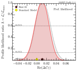
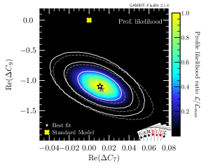
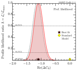
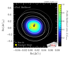
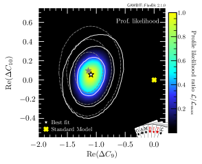
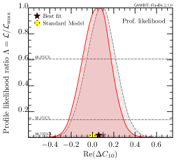
Figure 1: Complete results of the combined fit to the $\operatorname{Re}(\Delta C_{7})$, $\operatorname{Re}(\Delta C_{9})$ and $\operatorname{Re}(\Delta C_{10})$ Wilson coefficients, showing one- and two-dimensional profile likelihoods of each parameter. Contour lines indicate 1, 2 and 3$\sigma$ confidence regions. White contours and coloured shading in two-dimensional planes, and red one-dimensional curves, show our main results, where we compute theory covariances self-consistently for every combination of Wilson coefficients. Grey contours and curves show the corresponding result when we approximate the theory covariance by its value in the Standard Model, across the entire parameter space. The Standard Model prediction is indicated by a yellow cross.

5 Results

5.1 Current status

In Tab. 1 and Fig. 1 we present the main results of our global fit, providing one and two dimensional profile likelihoods for each of the Wilson coefficients. As can be seen, the strongest required modification to the SM Wilson coefficients is in $\operatorname{Re}(C_{9})$. The best-fit points correspond to coupling strengths $\operatorname{Re}(C_{7})/\operatorname{Re}(C_{7}^{\text{SM}})=0.96$, $\operatorname{Re}(C_{9})/\operatorname{Re}(C_{9}^{\text{SM}})=0.74$, and $\operatorname{Re}(C_{10})/\operatorname{Re}(C_{10}^{\text{SM}})=0.99$ relative to the SM. The agreement with the SM can be quantified by comparing the log-likelihood of the best-fit point to that of the SM. This gives a total of $\Delta\ln\mathcal{L}=25.8$, which for the three degrees of freedom in our fit, corresponds to a $6.6\sigma$ exclusion of the SM. Considering just $\operatorname{Re}(C_{9})$ alone, i.e. also profiling out the impacts of allowing $\operatorname{Re}(C_{7})$ and $\operatorname{Re}(C_{10})$ to vary, such that only a single degree of freedom remains, we find $\Delta\ln\mathcal{L}=19.6$. This corresponds to a $6.3\sigma$ preference for a non-SM value of $C_{9}$.

Previous analysis of older datasets in terms of the same Wilson coefficients have assumed that the covariance matrix describing the theoretical uncertainties on the observable predictions could be reliably approximated by its value computed for the SM, across the entire Wilson coefficient parameter space. In our fits, we have explicitly recomputed these theoretical uncertainties at every point in the Wilson coefficient parameter space. We show the impact of this improvement in Fig. 1, by indicating with a grey star and dashed grey curves the best fit and 1, 2 and $3\sigma$ confidence regions that would result from adopting the SM approximation. The central value is not strongly affected, but the impact upon the resulting confidence regions is non-negligible.

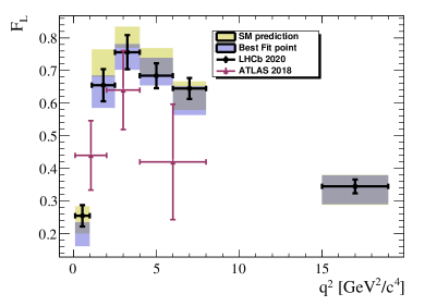
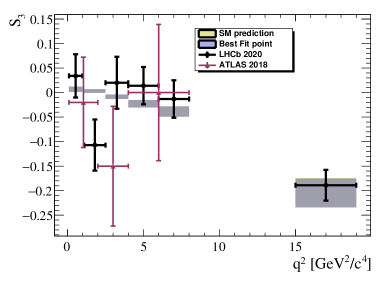
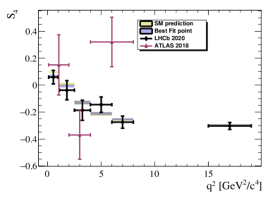
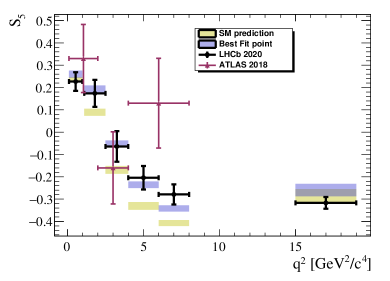
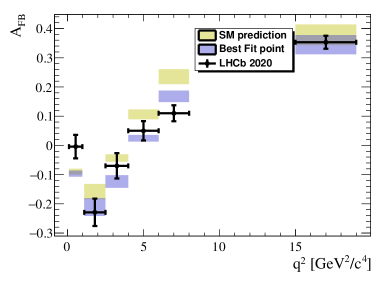
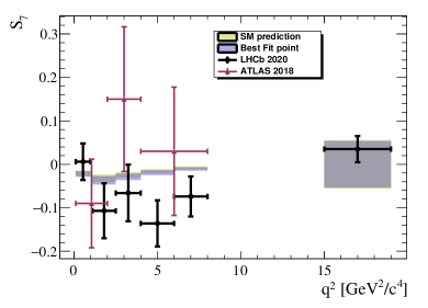
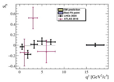
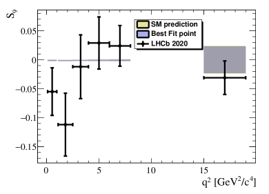
Figure 2: Angular observables for the decay $\mathit{{B}{}_{\mspace{-3.0mu}\scriptstyle{d}}^{\mspace{-1.0mu}\scriptstyle{}}}\to\mathit{{K}{}_{\mspace{-3.0mu}\scriptstyle{}}^{\mspace{-1.0mu}\scriptstyle{*0}}}\mathit{{\mu}{}_{\mspace{-3.0mu}\scriptstyle{}}^{\mspace{-1.0mu}\scriptstyle{+}}}\mathit{{\mu}{}_{\mspace{-3.0mu}\scriptstyle{}}^{\mspace{-1.0mu}\scriptstyle{-}}}$ included in our fit. Yellow shading corresponds to Standard Model predictions and uncertainties, and blue shading shows the prediction of our best-fit model. Data points with error bars show measurements from LHCb Aaij:2020nrf and ATLAS Aaboud:2018krd . For display purposes, we present theoretical predictions using the same binning as LHCb; in the likelihood function, we always compare experimental results to theory predictions computed in the same binning as used by the experiment in question.

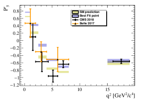
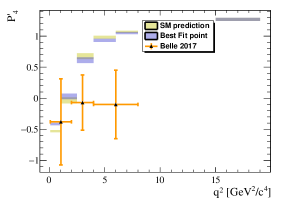
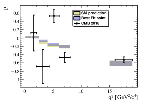
Figure 3: Optimised angular observables for the decay $\mathit{{B}{}_{\mspace{-3.0mu}\scriptstyle{d}}^{\mspace{-1.0mu}\scriptstyle{}}}\to\mathit{{K}{}_{\mspace{-3.0mu}\scriptstyle{}}^{\mspace{-1.0mu}\scriptstyle{*0}}}\mathit{{\mu}{}_{\mspace{-3.0mu}\scriptstyle{}}^{\mspace{-1.0mu}\scriptstyle{+}}}\mathit{{\mu}{}_{\mspace{-3.0mu}\scriptstyle{}}^{\mspace{-1.0mu}\scriptstyle{-}}}$ included in our fit. Yellow shading corresponds to Standard Model predictions and uncertainties, and blue shading shows the prediction of our best-fit model. Data points with error bars show measurements from Belle Wehle:2016yoi and CMS CMS:2017ivg . For display purposes, we again present the theoretical predictions using the LHCb binning in $q^{2}$, but consistently recompute the theory predictions in the bins used by Belle and CMS in order to determine their contributions to the overall likelihood.

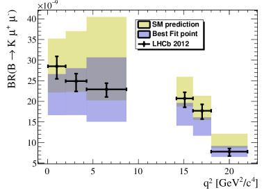
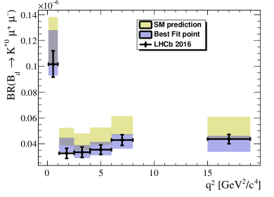
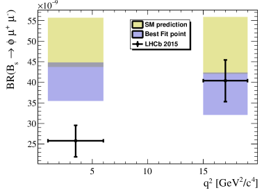
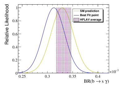
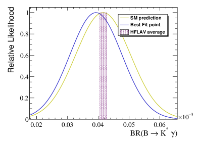
Figure 4: Branching fractions for $\mathit{{b}{}_{\mspace{-3.0mu}\scriptstyle{}}^{\mspace{-1.0mu}\scriptstyle{}}}\to\mathit{{s}{}_{\mspace{-3.0mu}\scriptstyle{}}^{\mspace{-1.0mu}\scriptstyle{}}}$ transitions included in our fit. Yellow shading corresponds to Standard Model predictions and uncertainties, and blue shading shows the prediction of our best-fit model. Data points with error bars show measurements from LHCb Aaij:2015esa ; Aaij:2016flj ; Aaij:2012vr . The $\mathit{{b}{}_{\mspace{-3.0mu}\scriptstyle{}}^{\mspace{-1.0mu}\scriptstyle{}}}\to\mathit{{s}{}_{\mspace{-3.0mu}\scriptstyle{}}^{\mspace{-1.0mu}\scriptstyle{}}}\mathit{{\gamma}{}_{\mspace{-3.0mu}\scriptstyle{}}^{\mspace{-1.0mu}\scriptstyle{}}}$ and ${\mathit{{B}{}_{\mspace{-3.0mu}\scriptstyle{}}^{\mspace{-1.0mu}\scriptstyle{}}}\to\mathit{{K}{}_{\mspace{-3.0mu}\scriptstyle{}}^{\mspace{-1.0mu}\scriptstyle{*0}}}\gamma}$ measurements are taken from HFLAV Amhis:2018udz .

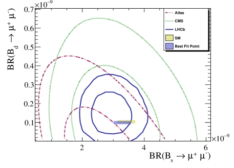
Figure 5: Branching fractions for $\mathit{{B}{}_{\mspace{-3.0mu}\scriptstyle{s}}^{\mspace{-1.0mu}\scriptstyle{}}}/\mathit{{B}{}_{\mspace{-3.0mu}\scriptstyle{d}}^{\mspace{-1.0mu}\scriptstyle{}}}\to\mathit{{\mu}{}_{\mspace{-3.0mu}\scriptstyle{}}^{\mspace{-1.0mu}\scriptstyle{+}}}\mathit{{\mu}{}_{\mspace{-3.0mu}\scriptstyle{}}^{\mspace{-1.0mu}\scriptstyle{-}}}$ decays included in our fit. Contour lines correspond to the joint 1 and 2$\sigma$ confidence regions obtained in the measurements by ATLAS Aaboud:2018mst , CMS CMS:2019qnb and LHCb Aaij:2017vad . Yellow shading corresponds to Standard Model predictions and uncertainties, and blue shading shows the prediction and uncertainty of our best-fit model.

In Figs. 2–5, we provide plots of the key observables and data that enter our fit. These consist of the $\mathit{{B}{}_{\mspace{-3.0mu}\scriptstyle{d}}^{\mspace{-1.0mu}\scriptstyle{}}}\to\mathit{{K}{}_{\mspace{-3.0mu}\scriptstyle{}}^{\mspace{-1.0mu}\scriptstyle{*0}}}\mathit{{\mu}{}_{\mspace{-3.0mu}\scriptstyle{}}^{\mspace{-1.0mu}\scriptstyle{+}}}\mathit{{\mu}{}_{\mspace{-3.0mu}\scriptstyle{}}^{\mspace{-1.0mu}\scriptstyle{-}}}$ angular observables in the $S_{i}$ basis (Fig. 2), their optimised versions (Fig. 3), branching fractions for other $b\to s$ processes (Fig. 4), and the joint measurement of the branching fractions of $\mathit{{B}{}_{\mspace{-3.0mu}\scriptstyle{s}}^{\mspace{-1.0mu}\scriptstyle{}}}\to\mathit{{\mu}{}_{\mspace{-3.0mu}\scriptstyle{}}^{\mspace{-1.0mu}\scriptstyle{+}}}\mathit{{\mu}{}_{\mspace{-3.0mu}\scriptstyle{}}^{\mspace{-1.0mu}\scriptstyle{-}}}$ and $\mathit{{B}{}_{\mspace{-3.0mu}\scriptstyle{d}}^{\mspace{-1.0mu}\scriptstyle{}}}\to\mathit{{\mu}{}_{\mspace{-3.0mu}\scriptstyle{}}^{\mspace{-1.0mu}\scriptstyle{+}}}\mathit{{\mu}{}_{\mspace{-3.0mu}\scriptstyle{}}^{\mspace{-1.0mu}\scriptstyle{-}}}$ (Fig. 5). We show the predictions of both the SM and our best-fit point, the theoretical uncertainties in each case, and the respective data from LHCb, ATLAS, CMS and Belle used in our fits. The improvement offered by the best-fit point is most visible in the $S_{5}$ and $A_{\rm FB}$ angular observables (Fig. 2), and in the overall branching fractions for $\mathit{{B}{}_{\mspace{-3.0mu}\scriptstyle{d}}^{\mspace{-1.0mu}\scriptstyle{}}}\to\mathit{{K}{}_{\mspace{-3.0mu}\scriptstyle{}}^{\mspace{-1.0mu}\scriptstyle{*0}}}\mathit{{\mu}{}_{\mspace{-3.0mu}\scriptstyle{}}^{\mspace{-1.0mu}\scriptstyle{+}}}\mathit{{\mu}{}_{\mspace{-3.0mu}\scriptstyle{}}^{\mspace{-1.0mu}\scriptstyle{-}}}$ and $\mathit{{B}{}_{\mspace{-3.0mu}\scriptstyle{s}}^{\mspace{-1.0mu}\scriptstyle{}}}\to\mathit{{\phi}{}_{\mspace{-3.0mu}\scriptstyle{}}^{\mspace{-1.0mu}\scriptstyle{}}}\mathit{{\mu}{}_{\mspace{-3.0mu}\scriptstyle{}}^{\mspace{-1.0mu}\scriptstyle{+}}}\mathit{{\mu}{}_{\mspace{-3.0mu}\scriptstyle{}}^{\mspace{-1.0mu}\scriptstyle{-}}}$ decays (Fig. 4). Some reduction is expected in the branching fractions for $\mathit{{b}{}_{\mspace{-3.0mu}\scriptstyle{}}^{\mspace{-1.0mu}\scriptstyle{}}}\to\mathit{{s}{}_{\mspace{-3.0mu}\scriptstyle{}}^{\mspace{-1.0mu}\scriptstyle{}}}\mathit{{\gamma}{}_{\mspace{-3.0mu}\scriptstyle{}}^{\mspace{-1.0mu}\scriptstyle{}}}$ and ${\mathit{{B}{}_{\mspace{-3.0mu}\scriptstyle{}}^{\mspace{-1.0mu}\scriptstyle{}}}\to\mathit{{K}{}_{\mspace{-3.0mu}\scriptstyle{}}^{\mspace{-1.0mu}\scriptstyle{*0}}}\gamma}$ relative to the SM in our best-fit model (Fig. 4), owing to the small positive best-fit value of $\operatorname{Re}(C_{7})$ (recalling that the SM value of $C_{7}$ is negative). These are however sufficiently small that the predictions remain consistent with the HFLAV value Amhis:2018udz .

5.2 Implications for future searches

With higher precision measurements of $\mathit{{B}{}_{\mspace{-3.0mu}\scriptstyle{d}}^{\mspace{-1.0mu}\scriptstyle{}}}\to\mathit{{K}{}_{\mspace{-3.0mu}\scriptstyle{}}^{\mspace{-1.0mu}\scriptstyle{*0}}}\mathit{{\mu}{}_{\mspace{-3.0mu}\scriptstyle{}}^{\mspace{-1.0mu}\scriptstyle{+}}}\mathit{{\mu}{}_{\mspace{-3.0mu}\scriptstyle{}}^{\mspace{-1.0mu}\scriptstyle{-}}}$ in the future, Wilson coefficient fits will of course increase in precision. There are however also ongoing efforts to extract the non-factorisable contributions directly from $\mathit{{B}{}_{\mspace{-3.0mu}\scriptstyle{d}}^{\mspace{-1.0mu}\scriptstyle{}}}\to\mathit{{K}{}_{\mspace{-3.0mu}\scriptstyle{}}^{\mspace{-1.0mu}\scriptstyle{*0}}}\mathit{{\mu}{}_{\mspace{-3.0mu}\scriptstyle{}}^{\mspace{-1.0mu}\scriptstyle{+}}}\mathit{{\mu}{}_{\mspace{-3.0mu}\scriptstyle{}}^{\mspace{-1.0mu}\scriptstyle{-}}}$ data Mauri:2018vbg . The Belle II experiment has recently started taking data as well, with the aim of eventually reaching $50~{}\rm{ab}^{-1}$ integrated luminosity. The unprecedented number of decays that will be contained in this dataset creates the possibility to measure the branching fraction for inclusive $\mathit{{B}{}_{\mspace{-3.0mu}\scriptstyle{}}^{\mspace{-1.0mu}\scriptstyle{}}}\to X_{s}\mathit{{\mu}{}_{\mspace{-3.0mu}\scriptstyle{}}^{\mspace{-1.0mu}\scriptstyle{+}}}\mathit{{\mu}{}_{\mspace{-3.0mu}\scriptstyle{}}^{\mspace{-1.0mu}\scriptstyle{-}}}$ decays. In Fig. 6, we show the predictions for $BR(\mathit{{B}{}_{\mspace{-3.0mu}\scriptstyle{}}^{\mspace{-1.0mu}\scriptstyle{}}}\to X_{s}\mathit{{\mu}{}_{\mspace{-3.0mu}\scriptstyle{}}^{\mspace{-1.0mu}\scriptstyle{+}}}\mathit{{\mu}{}_{\mspace{-3.0mu}\scriptstyle{}}^{\mspace{-1.0mu}\scriptstyle{-}}})$ in our best-fit model and in the SM, for two example $q^{2}$ ranges. We overlay an expected Belle II measurement, with the central value set to our best-fit prediction and the uncertainty band based on the predicted sensitivity of Ref. Kou:2018nap . Belle II will clearly have sufficient sensitivity in the low-$q^{2}$ region to strongly distinguish the best-fit point from the SM.

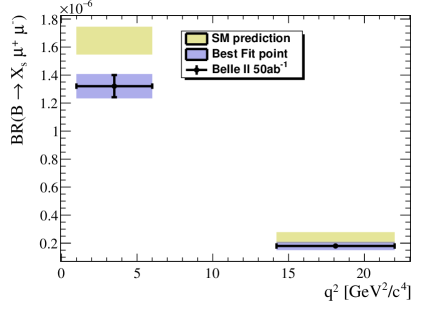
Figure 6: Predicted exclusive branching fraction $BR(\mathit{{B}{}_{\mspace{-3.0mu}\scriptstyle{}}^{\mspace{-1.0mu}\scriptstyle{}}}\to X_{s}\mathit{{\mu}{}_{\mspace{-3.0mu}\scriptstyle{}}^{\mspace{-1.0mu}\scriptstyle{+}}}\mathit{{\mu}{}_{\mspace{-3.0mu}\scriptstyle{}}^{\mspace{-1.0mu}\scriptstyle{-}}})$ in the Standard model (yellow shading) and in our best-fit model (blue shading). We also show the expected sensitivity of Belle II after it has collected 50 ab^-1 of data Kou:2018nap , assuming that the central measured values are equal to our best-fit prediction.

6 Conclusions

We have used the FlavBit module of the GAMBIT package to perform a simultaneous fit of the real parts of the Wilson coefficients $C_{7}$, $C_{9}$ and $C_{10}$, using combined data on $\mathit{{b}{}_{\mspace{-3.0mu}\scriptstyle{}}^{\mspace{-1.0mu}\scriptstyle{}}}\to\mathit{{s}{}_{\mspace{-3.0mu}\scriptstyle{}}^{\mspace{-1.0mu}\scriptstyle{}}}\mathit{{\mu}{}_{\mspace{-3.0mu}\scriptstyle{}}^{\mspace{-1.0mu}\scriptstyle{+}}}\mathit{{\mu}{}_{\mspace{-3.0mu}\scriptstyle{}}^{\mspace{-1.0mu}\scriptstyle{-}}}$ transitions. Our results show that measurements of flavour anomalies in this sector have reached an intriguing historical juncture, as they are now sufficiently persistent that their tension with the SM increases steadily as new data are collected. With the inclusion of recently updated results from the LHCb collaboration, we find best-fit values relative to the SM predictions of $\operatorname{Re}(C_{7})/\operatorname{Re}(C_{7}^{\text{SM}})=0.96$, $\operatorname{Re}(C_{9})/\operatorname{Re}(C_{9}^{\text{SM}})=0.74$, and $\operatorname{Re}(C_{10})/\operatorname{Re}(C_{10}^{\text{SM}})=0.99$. Performing a hypothesis test of the SM by comparing the log-likelihood of our best-fit point to that of the SM, we obtain a $6.6\sigma$ preference for our best-fit point over the SM. This reduces slightly to $6.3\sigma$ when $C_{7}$ and $C_{10}$ are profiled out. By explicitly recomputing the theoretical uncertainty covariance matrix at every point in the Wilson coefficient parameter space, we have shown that the best-fit value is not strongly affected by departing from the usual assumption of an SM-only calculation, but that the effect is important for correctly determining confidence intervals, and therefore the overall significance of the result. Our results still rely on our specific choice of parameterisation of the non-factorisable QCD corrections to many key observables, but the more accurate treatment that we employ of the theory uncertainties across the Wilson coefficient parameter space is an important step forward in improving the test of the SM hypothesis.

Inspection of the observables that entered our fit indicate that our best-fit point better matches measurements of the $S_{5}$ and $A_{FB}$ observables than the SM, in addition to the overall branching fractions for $\mathit{{B}{}_{\mspace{-3.0mu}\scriptstyle{d}}^{\mspace{-1.0mu}\scriptstyle{}}}\to\mathit{{K}{}_{\mspace{-3.0mu}\scriptstyle{}}^{\mspace{-1.0mu}\scriptstyle{*0}}}\mathit{{\mu}{}_{\mspace{-3.0mu}\scriptstyle{}}^{\mspace{-1.0mu}\scriptstyle{+}}}\mathit{{\mu}{}_{\mspace{-3.0mu}\scriptstyle{}}^{\mspace{-1.0mu}\scriptstyle{-}}}$ and $\mathit{{B}{}_{\mspace{-3.0mu}\scriptstyle{s}}^{\mspace{-1.0mu}\scriptstyle{}}}\to\mathit{{\phi}{}_{\mspace{-3.0mu}\scriptstyle{}}^{\mspace{-1.0mu}\scriptstyle{}}}\mathit{{\mu}{}_{\mspace{-3.0mu}\scriptstyle{}}^{\mspace{-1.0mu}\scriptstyle{+}}}\mathit{{\mu}{}_{\mspace{-3.0mu}\scriptstyle{}}^{\mspace{-1.0mu}\scriptstyle{-}}}$ decays. Other observables are less strongly affected. Localisation of the apparent new physics contribution in a shift of the $C_{9}$ Wilson coefficient means that the physics should result from a vector coupling of $b$ and $s$ quarks to muons.

References

- (1) S. L. Glashow, J. Iliopoulos, and L. Maiani, Weak interactions with lepton-hadron symmetry, Phys. Rev. D 2 (1970) 1285–1292.
- (2) LHCb Collaboration: R. Aaij et. al., Measurement of Form-Factor-Independent Observables in the Decay , Phys. Rev. Lett. 111 (2013) 191801, [arXiv:1308.1707].
- (3) LHCb Collaboration: R. Aaij et. al., Differential branching fraction and angular analysis of the decay , JHEP 07 (2013) 084, [arXiv:1305.2168].
- (4) LHCb Collaboration: R. Aaij et. al., Branching Fraction Measurements of the Rare and - Decays, Phys. Rev. Lett. 127 (2021) 151801, [arXiv:2105.14007].
- (5) LHCb Collaboration: R. Aaij et. al., Measurement of the phase difference between short- and long-distance amplitudes in the decay, Eur. Phys. J. C 77 (2017) 161, [arXiv:1612.06764].
- (6) LHCb Collaboration: R. Aaij et. al., Differential branching fraction and angular analysis of decays, JHEP 06 (2015) 115, [arXiv:1503.07138]. [Erratum: JHEP 09, 145 (2018)].
- (7) Belle Collaboration: A. Abdesselam et. al., Angular analysis of , in A First Discussion of 13 TeV Results: Obergurgl, Austria, April 10-15, 2016, Proceedings of LHC Ski 2016 (2016) [arXiv:1604.04042].
- (8) ATLAS Collaborations: M. Aaboud et. al., Angular analysis of decays in collisions at TeV with the ATLAS detector, JHEP 10 (2018) 047, [arXiv:1805.04000].
- (9) CMS Collaboration: A. M. Sirunyan et. al., Measurement of angular parameters from the decay in proton-proton collisions at 8 TeV, Phys. Lett. B 781 (2018) 517–541, [arXiv:1710.02846].
- (10) G. D’Amico, M. Nardecchia, et. al., Flavour anomalies after the measurement, JHEP 09 (2017) 010, [arXiv:1704.05438].
- (11) L.-S. Geng, B. Grinstein, et. al., Towards the discovery of new physics with lepton-universality ratios of decays, Phys. Rev. D 96 (2017) 093006, [arXiv:1704.05446].
- (12) T. Hurth, F. Mahmoudi, D. Martinez Santos, and S. Neshatpour, Lepton nonuniversality in exclusive decays, Phys. Rev. D 96 (2017) 095034, [arXiv:1705.06274].
- (13) M. Algueró, B. Capdevila, et. al., Emerging patterns of New Physics with and without Lepton Flavour Universal contributions, Eur. Phys. J. C 79 (2019) 714, [arXiv:1903.09578].
- (14) A. K. Alok, A. Dighe, S. Gangal, and D. Kumar, Continuing search for new physics in decays: two operators at a time, JHEP 06 (2019) 089, [arXiv:1903.09617].
- (15) M. Ciuchini, A. M. Coutinho, et. al., New Physics in confronts new data on Lepton Universality, Eur. Phys. J. C 79 (2019) 719, [arXiv:1903.09632].
- (16) J. Aebischer, W. Altmannshofer, et. al., B-decay discrepancies after Moriond 2019, Eur. Phys. J. C 80 (2020) 252, [arXiv:1903.10434].
- (17) K. Kowalska, D. Kumar, and E. M. Sessolo, Implications for new physics in transitions after recent measurements by Belle and LHCb, Eur. Phys. J. C 79 (2019) 840, [arXiv:1903.10932].
- (18) A. Arbey, T. Hurth, F. Mahmoudi, and S. Neshatpour, Hadronic and New Physics Contributions to Transitions, Phys. Rev. D 98 (2018) 095027, [arXiv:1806.02791].
- (19) A. Datta, J. Kumar, and D. London, The anomalies and new physics in , Phys. Lett. B 797 (2019) 134858, [arXiv:1903.10086].
- (20) A. Arbey, T. Hurth, F. Mahmoudi, D. M. Santos, and S. Neshatpour, Update on the bs anomalies, Phys. Rev. D 100 (2019) 015045, [arXiv:1904.08399].
- (21) A. Khodjamirian, T. Mannel, A. Pivovarov, and Y.-M. Wang, Charm-loop effect in and , JHEP 09 (2010) 089, [arXiv:1006.4945].
- (22) A. Khodjamirian, T. Mannel, and Y. Wang, decay at large hadronic recoil, JHEP 02 (2013) 010, [arXiv:1211.0234].
- (23) M. Dimou, J. Lyon, and R. Zwicky, Exclusive Chromomagnetism in heavy-to-light FCNCs, Phys. Rev. D 87 (2013) 074008, [arXiv:1212.2242].
- (24) J. Lyon and R. Zwicky, Isospin asymmetries in and in and beyond the standard model, Phys. Rev. D 88 (2013) 094004, [arXiv:1305.4797].
- (25) J. Lyon and R. Zwicky, Resonances gone topsy turvy - the charm of QCD or new physics in ?, arXiv:1406.0566.
- (26) C. Bobeth, M. Chrzaszcz, D. van Dyk, and J. Virto, Long-distance effects in from analyticity, Eur. Phys. J. C 78 (2018) 451, [arXiv:1707.07305].
- (27) T. Blake, U. Egede, P. Owen, K. A. Petridis, and G. Pomery, An empirical model to determine the hadronic resonance contributions to transitions, Eur. Phys. J. C 78 (2018) 453, [arXiv:1709.03921].
- (28) T. Hurth, F. Mahmoudi, and S. Neshatpour, On the new LHCb angular analysis of : Hadronic effects or New Physics?, Phys. Rev. D 102 (2020) 055001, [arXiv:2006.04213].
- (29) LHCb Collaboration: R. Aaij et. al., Test of lepton universality in beauty-quark decays, arXiv:2103.11769.
- (30) LHCb Collaboration: R. Aaij et. al., Test of lepton universality with decays, JHEP 08 (2017) 055, [arXiv:1705.05802].
- (31) The GAMBIT Flavour Workgroup: F. U. Bernlochner et. al., FlavBit: A GAMBIT module for computing flavour observables and likelihoods, Eur. Phys. J. C 77 (2017) 786, [arXiv:1705.07933].
- (32) GAMBIT Collaboration: P. Athron et. al., GAMBIT: The Global and Modular Beyond-the-Standard-Model Inference Tool, Eur. Phys. J. C 77 (2017) 784, [arXiv:1705.07908]. [Addendum: Eur. Phys. J. C 78, 98 (2018)].
- (33) A. Kvellestad, P. Scott, and M. White, GAMBIT and its Application in the Search for Physics Beyond the Standard Model, Prog. Part. Nuc. Phys. in press (2020) [arXiv:1912.04079].
- (34) F. Mahmoudi, SuperIso: A Program for calculating the isospin asymmetry of in the MSSM, Comp. Phys. Comm. 178 (2008) 745, [arXiv:0710.2067].
- (35) F. Mahmoudi, SuperIso v2.3: A Program for calculating flavor physics observables in Supersymmetry, Comp. Phys. Comm. 180 (2009) 1579, [arXiv:0808.3144].
- (36) F. Mahmoudi, SuperIso v3.0, flavor physics observables calculations: Extension to NMSSM, Comp. Phys. Comm. 180 (2009) 1718.
- (37) U. Egede, T. Hurth, J. Matias, M. Ramon, and W. Reece, New observables in the decay mode , JHEP 11 (2008) 032, [arXiv:0807.2589].
- (38) U. Egede, T. Hurth, J. Matias, M. Ramon, and W. Reece, New physics reach of the decay mode , JHEP 10 (2010) 056, [arXiv:1005.0571].
- (39) A. Bharucha, D. M. Straub, and R. Zwicky, in the Standard Model from light-cone sum rules, JHEP 08 (2016) 098, [arXiv:1503.05534].
- (40) M. Beneke, T. Feldmann, and D. Seidel, Exclusive radiative and electroweak and penguin decays at NLO, Eur. Phys. J. C 41 (2005) 173–188, [hep-ph/0412400].
- (41) T. Hurth, F. Mahmoudi, and S. Neshatpour, On the anomalies in the latest LHCb data, Nucl. Phys. B 909 (2016) 737–777, [arXiv:1603.00865].
- (42) V. Chobanova, T. Hurth, F. Mahmoudi, D. Martinez Santos, and S. Neshatpour, Large hadronic power corrections or new physics in the rare decay ?, JHEP 07 (2017) 025, [arXiv:1702.02234].
- (43) J. Matias, F. Mescia, M. Ramon, and J. Virto, Complete Anatomy of and its angular distribution, JHEP 04 (2012) 104, [arXiv:1202.4266].
- (44) S. Descotes-Genon, T. Hurth, J. Matias, and J. Virto, Optimizing the basis of observables in the full kinematic range, JHEP 05 (2013) 137, [arXiv:1303.5794].
- (45) R. Sinha, CP violation in B mesons using Dalitz plot asymmetries, hep-ph/9608314.
- (46) F. Kruger, L. M. Sehgal, N. Sinha, and R. Sinha, Angular distribution and CP asymmetries in the decays and , Phys. Rev. D 61 (2000) 114028, [hep-ph/9907386]. [Erratum: Phys. Rev. D63, 019901 (2001)].
- (47) W. Altmannshofer, P. Ball, et. al., Symmetries and Asymmetries of Decays in the Standard Model and Beyond, JHEP 01 (2009) 019, [arXiv:0811.1214].
- (48) LHCb Collaboration: R. Aaij et. al., Measurement of -averaged observables in the decay, Phys. Rev. Lett. 125 (2020) 011802, [arXiv:2003.04831].
- (49) J. Gratrex, M. Hopfer, and R. Zwicky, Generalised helicity formalism, higher moments and the angular distributions, Phys. Rev. D 93 (2016) 054008, [arXiv:1506.03970].
- (50) Belle Collaboration: S. Wehle et. al., Lepton-Flavor-Dependent Angular Analysis of , Phys. Rev. Lett. 118 (2017) 111801, [arXiv:1612.05014].
- (51) LHCb Collaboration: R. Aaij et. al., Differential branching fraction and angular analysis of the decay , JHEP 08 (2013) 131, [arXiv:1304.6325].
- (52) LHCb Collaboration: R. Aaij et. al., Measurements of the S-wave fraction in decays and the differential branching fraction, JHEP 11 (2016) 047, [arXiv:1606.04731]. [Erratum: JHEP 04, 142 (2017)].
- (53) LHCb Collaboration: R. Aaij et. al., Angular analysis and differential branching fraction of the decay , JHEP 09 (2015) 179, [arXiv:1506.08777].
- (54) S. Descotes-Genon and J. Virto, Time dependence in decays, JHEP 04 (2015) 045, [arXiv:1502.05509]. [Erratum: JHEP 07, 049 (2015)].
- (55) Particle Data Group: M. Tanabashi et. al., Review of particle physics, Phys. Rev. D 98 (2018) 030001.
- (56) LHCb Collaboration: R. Aaij et. al., Differential branching fraction and angular analysis of the decay, JHEP 02 (2013) 105, [arXiv:1209.4284].
- (57) BaBar Collaboration: B. Aubert et. al., Direct CP, Lepton Flavor and Isospin Asymmetries in the Decays , Phys. Rev. Lett. 102 (2009) 091803, [arXiv:0807.4119].
- (58) Belle Collaboration: J.-T. Wei et. al., Measurement of the Differential Branching Fraction and Forward-Backword Asymmetry for , Phys. Rev. Lett. 103 (2009) 171801, [arXiv:0904.0770].
- (59) C. Bobeth, G. Hiller, and G. Piranishvili, Angular distributions of decays, JHEP 12 (2007) 040, [arXiv:0709.4174].
- (60) D. Becirevic, N. Kosnik, F. Mescia, and E. Schneider, Complementarity of the constraints on New Physics from and from decays, Phys. Rev. D 86 (2012) 034034, [arXiv:1205.5811].
- (61) W. Altmannshofer and D. M. Straub, New physics in transitions after LHC run 1, Eur. Phys. J. C 75 (2015) 382, [arXiv:1411.3161].
- (62) M. Beneke, T. Feldmann, and D. Seidel, Systematic approach to exclusive , decays, Nucl. Phys. B 612 (2001) 25–58, [hep-ph/0106067].
- (63) Flavour Lattice Averaging Group: S. Aoki et. al., FLAG Review 2019: Flavour Lattice Averaging Group (FLAG), Eur. Phys. J. C 80 (2020) 113, [arXiv:1902.08191].
- (64) R. Grigjanis, P. J. O’Donnell, M. Sutherland, and H. Navelet, QCD Corrected Effective Lagrangian for B s Processes, Phys. Lett. B 213 (1988) 355. [Erratum: Phys.Lett.B 286, 413 (1992)].
- (65) B. Grinstein, R. P. Springer, and M. B. Wise, Effective Hamiltonian for Weak Radiative B Meson Decay, Phys. Lett. B 202 (1988) 138–144.
- (66) M. Misiak et. al., Estimate of at , Phys. Rev. Lett. 98 (2007) 022002, [hep-ph/0609232].
- (67) M. Misiak and M. Steinhauser, NNLO QCD corrections to the anti-B X(s) gamma matrix elements using interpolation in m(c), Nucl. Phys. B 764 (2007) 62–82, [hep-ph/0609241].
- (68) M. Czakon, P. Fiedler, et. al., The contribution to at , JHEP 04 (2015) 168, [arXiv:1503.01791].
- (69) M. Misiak, A. Rehman, and M. Steinhauser, NNLO QCD counterterm contributions to for the physical value of , Phys. Lett. B 770 (2017) 431–439, [arXiv:1702.07674].
- (70) M. Misiak, A. Rehman, and M. Steinhauser, Towards at the NNLO in QCD without interpolation in , JHEP 06 (2020) 175, [arXiv:2002.01548].
- (71) A. Czarnecki and W. J. Marciano, Electroweak radiative corrections to b s gamma, Phys. Rev. Lett. 81 (1998) 277–280, [hep-ph/9804252].
- (72) A. Gunawardana and G. Paz, Reevaluating uncertainties in decay, JHEP 11 (2019) 141, [arXiv:1908.02812].
- (73) LHCb Collaboration: R. Aaij et. al., Observation of the suppressed decay , JHEP 04 (2017) 029, [arXiv:1701.08705].
- (74) LHCb Collaboration: R. Aaij et. al., Angular moments of the decay at low hadronic recoil, JHEP 09 (2018) 146, [arXiv:1808.00264].
- (75) T. Blake and M. Kreps, Angular distribution of polarised baryons decaying to , JHEP 11 (2017) 138, [arXiv:1710.00746].
- (76) F. Beaujean, M. Chrza̧szcz, N. Serra, and D. van Dyk, Extracting Angular Observables without a Likelihood and Applications to Rare Decays, Phys. Rev. D 91 (2015) 114012, [arXiv:1503.04100].
- (77) W. Detmold and S. Meinel, form factors, differential branching fraction, and angular observables from lattice QCD with relativistic quarks, Phys. Rev. D 93 (2016) 074501, [arXiv:1602.01399].
- (78) J. Bhom and M. Chrzaszcz, HEPLike: an open source framework for experimental likelihood evaluation, Comput. Phys. Commun. 254 (2020) 107235, [arXiv:2003.03956].
- (79) J. Bhom and M. Chrza̧szcz, HEPLikeData, 2020. https://github.com/mchrzasz/HEPLikeData.
- (80) GAMBIT Scanner Workgroup: G. D. Martinez, J. McKay, et. al., Comparison of statistical sampling methods with ScannerBit, the GAMBIT scanning module, Eur. Phys. J. C 77 (2017) 761, [arXiv:1705.07959].
- (81) A. Arbey, S. Fichet, F. Mahmoudi, and G. Moreau, The correlation matrix of Higgs rates at the LHC, JHEP 11 (2016) 097, [arXiv:1606.00455].
- (82) LHCb Collaboration: R. Aaij et. al., Angular analysis of the decay using 3 fb-1 of integrated luminosity, JHEP 02 (2016) 104, [arXiv:1512.04442].
- (83) CMS Collaboration, Measurement of the and angular parameters of the decay in proton-proton collisions at , CMS-PAS-BPH-15-008, 2017.
- (84) LHCb Collaboration: R. Aaij et. al., Angular Analysis of the Decay, Phys. Rev. Lett. 126 (2021) 161802, [arXiv:2012.13241].
- (85) LHCb Collaboration: R. Aaij et. al., Measurement of the branching fraction and effective lifetime and search for decays, Phys. Rev. Lett. 118 (2017) 191801, [arXiv:1703.05747].
- (86) CMS Collaboration, Measurement of properties of decays and search for with the CMS experiment, CMS-PAS-BPH-16-004, 2019.
- (87) ATLAS Collaboration: M. Aaboud et. al., Study of the rare decays of and mesons into muon pairs using data collected during 2015 and 2016 with the ATLAS detector, JHEP 04 (2019) 098, [arXiv:1812.03017].
- (88) HFLAV Collaboration: Y. Amhis et. al., HFLAV input to the update of the European Strategy for Particle Physics, arXiv:1812.07461.
- (89) LHCb Collaboration: R. Aaij et. al., Strong constraints on the photon polarisation from decays, JHEP 12 (2020) 081, [arXiv:2010.06011].
- (90) A. Mauri, N. Serra, and R. Silva Coutinho, Towards establishing lepton flavor universality violation in decays, Phys. Rev. D 99 (2019) 013007, [arXiv:1805.06401].
- (91) Belle-II Collaboration: W. Altmannshofer et. al., The Belle II Physics Book, PTEP 2019 (2019) 123C01, [arXiv:1808.10567]. [Erratum: PTEP 2020, 029201 (2020)].
- (92) P. Scott, Pippi – painless parsing, post-processing and plotting of posterior and likelihood samples, Eur. Phys. J. Plus 127 (2012) 138, [arXiv:1206.2245].