Hierarchy of magnon entanglement in antiferromagnets

Abstract

Continuous variable entanglement between magnon modes in Heisenberg antiferromagnet with Dzyaloshinskii-Moryia (DM) interaction is examined. Different bosonic modes are identified, which allows to establish a hierarchy of magnon entanglement in the ground state. We argue that entanglement between magnon modes is determined by a simple lattice specific factor, together with the ratio of the strengths of the DM and Heisenberg exchange interactions, and that magnon entanglement can be detected by means of quantum homodyne techniques. As an illustration of the relevance of our findings for possible entanglement experiments in the solid state, a typical antiferromagnet with the perovskite crystal structure is considered, and it is shown that long wave length magnon modes have the highest degree of entanglement.

Quantum entanglement allows particles to act as a single non-separable entity, no matter how far apart they are. This is the feature that was initially used in the Einstein- Podolsky- Rosen (EPR) argument against completeness of quantum mechanics einstein35 . The original form of the EPR argument is closely related to continuous variable (CV) entanglement ou1992 ; giedke03 ; reid09 , which describes entanglement between bosonic modes. Such systems are characterized by an infinite number of allowed states, which makes them very different from the finite-dimensional Hilbert spaces associated with discrete variable (e.g., qubit) systems. Nevertheless, just as discrete variable entanglement, CV entanglement provides an essential resource for quantum technologies allowing for universal quantum information processing braunstein2005 , the realization of quantum teleportation braunstein2005 ; braunstein1998 ; Opatrny2001 , quantum memories braunstein2005 ; hammerer2010 , and quantum enhanced measurement resolution giovannetti2004 .

It is natural to expect that quantum systems, in which information is carried in a wave-like form, in general can show entanglement. However, the question is how clear the entanglement can be demonstrated and what quantum systems might be appropriate for potential applications. In the solid state, there are several collective modes that could be suitable hosts of entanglement. Here, we focus on magnons, collective wave-like excitations of a magnet with a well-established quantum nature mohn2006 . Typically magnons can be found in energy range of up to $\sim$ 500 meV, and with wave lengths spanning a range of hundreds of lattice constants to just a few. Low energy magnon excitations can be observed in different classes of magnetic materials, such as ferromagnets, antiferromagnets, and ferrimagnets, and each class has a vast space of materials to choose from. One of the broadest classes of antiferromagnets can be found in oxide compounds, in particular transition metal oxides googenough2020 , where for long wave lengths the dispersion relation is essentially linear.

In this paper, we focus on magnon CV entanglement in antiferromagnets, in which both the Heisenberg exchange and the Dzyaloshinskii-Moriya (DM) interactions may be relevant mohn2006 . To begin with, we consider the quantum antiferromagnetic Heisenberg Hamiltonian on a bipartite lattice

$$H_{0}=J\sum_{\langle ij\rangle}{\bf S}_{i}\cdot{\bf S}_{j},\ \ \ J>0,$$ (1)

where ${\bf S}_{j}$ is the spin-$S$ operator on site $j$ and $J$ is the strength of the exchange interaction. Using the Holstein-Primakoff (HP) transformation at low temperatures ($k_{B}T\ll J$) followed by the Fourier transformation, one can express the spin Hamiltonian (trivial terms and zero-point energies are neglected from now on) in terms of bosonic operators as

$$H_{0}=zJS\sum_{\mathbf{k}}\left[a_{\mathbf{k}}^{\dagger}a_{\mathbf{k}}+b_{\mathbf{k}}^{\dagger}b_{\mathbf{k}}+\gamma_{\mathbf{k}}a_{\mathbf{k}}b_{\mathbf{k}}+\gamma_{-\mathbf{k}}a_{\mathbf{k}}^{\dagger}b_{\mathbf{k}}^{\dagger}\right]$$ (2)

with the lattice specific parameter $\gamma_{\mathbf{k}}=\frac{1}{z}\sum_{\mathbf{\mathbf{\delta}}}e^{i\mathbf{k}\cdot\boldsymbol{\delta}}$, $z$ being the coordination number of the lattice and the sum over $\boldsymbol{\delta}$ is carried out over nearest neighbors. Here, $a_{\mathbf{k}}^{\dagger}$ ($a_{\mathbf{k}}$) and $b_{\mathbf{k}}^{\dagger}$ ($b_{\mathbf{k}}$) are bosonic creation (annihilation) operators representing two magnon modes with wave vector $\mathbf{k}$ that are associated with the two sublattices (see Supplemental Material).

By employing the Bogoliubov transformation

$$\left(\begin{array}[]{cc}a_{\mathbf{k}}\\ b_{\mathbf{k}}^{\dagger}\end{array}\right)=\left(\begin{array}[]{cc}u_{\mathbf{k}}&v_{\mathbf{k}}\\ v_{\mathbf{k}}^{*}&u^{*}_{\mathbf{k}}\end{array}\right)\left(\begin{array}[]{cc}\alpha_{\mathbf{k}}\\ \beta_{\mathbf{k}}^{\dagger}\end{array}\right),$$ (9)

with $u_{\mathbf{k}}$ and $v_{\mathbf{k}}$ given by

$$|u_{\mathbf{k}}|^{2} = \frac{1}{2\sqrt{1-|\gamma_{\mathbf{k}}|^{2}}}+\frac{1}{2},\ \ |v_{\mathbf{k}}|^{2}=\frac{1}{2\sqrt{1-|\gamma_{\mathbf{k}}|^{2}}}-\frac{1}{2},$$ (10)

$$\frac{v_{\mathbf{k}}}{u^{*}_{\mathbf{k}}}=-\frac{1-\sqrt{1-|\gamma_{\mathbf{k}}|^{2}}}{\gamma_{\mathbf{k}}},$$

where $|\gamma_{\mathbf{k}}|<1$, we obtain the Hamiltonian in diagonal form

$$H_{0}=\sum_{\mathbf{k}}\epsilon_{\mathbf{k}}(\alpha_{\mathbf{k}}^{\dagger}\alpha_{\mathbf{k}}+\beta_{\mathbf{k}}^{\dagger}\beta_{\mathbf{k}})$$ (11)

in terms of the new bosonic operators $(\alpha,\beta)$. For the antiferromagnetic magnon dispersion relation, we find $\epsilon_{\mathbf{k}}=zSJ\sqrt{(1-|\gamma_{\mathbf{k}}|^{2})}$ (see Supplemental Material for derivation).

The ground state of $H_{0}$ in the $(\alpha,\beta)$ modes reads $|\psi_{0}\rangle=\prod_{\mathbf{k}}|0;\alpha_{\mathbf{k}}\rangle|0;\beta_{\mathbf{k}}\rangle$, which is a separable vacuum state with vanishing entropy of entanglement remark1 , i.e., $E_{0}^{(\alpha,\beta)}=0$. By making the inverse Bogoliubov transformation, we may express the ground state as

$$|\psi_{0}\rangle=\prod_{\mathbf{k}}|r_{\mathbf{k}},\phi_{\mathbf{k}}\rangle$$ (12)

with the two-mode generalized coherent state

$$|r_{\mathbf{k}},\phi_{\mathbf{k}}\rangle=\frac{1}{\cosh r_{\mathbf{k}}}\sum_{n=0}^{\infty}e^{in\phi_{\mathbf{k}}}\tanh^{n}r_{\mathbf{k}}|n;a_{\mathbf{k}}\rangle|n;b_{\mathbf{k}}\rangle$$ (13)

in the $(a,b)$ occupation number basis $|n;a_{\mathbf{k}}\rangle$ and $|n;b_{\mathbf{k}}\rangle$ (see Supplemental Material for derivation). Here, the parameter $r_{\mathbf{k}}$ and the phase $\phi_{\mathbf{k}}$ are given by $e^{i\phi_{\mathbf{k}}}\tanh r_{\mathbf{k}}=\frac{v_{\mathbf{k}}}{u^{*}_{\mathbf{k}}}$, $r_{\mathbf{k}}\equiv r_{\mathbf{k}}(|\gamma_{\bf k}|)\geqslant 0$ and $\phi_{\mathbf{k}}\equiv\phi_{\mathbf{k}}(\gamma_{\bf k})=\pi-\arg[\gamma_{\mathbf{k}}]$. The entropy of entanglement for $|r_{\mathbf{k}},\phi_{\mathbf{k}}\rangle$ giedke03 ; remark1

$$E_{0}^{(a,b)} = \cosh^{2}r_{\mathbf{k}}\log_{2}\left[\cosh^{2}r_{\mathbf{k}}\right]-\sinh^{2}r_{\mathbf{k}}\log_{2}\left[\sinh^{2}r_{\mathbf{k}}\right]$$ (14)

$$= |u_{\mathbf{k}}|^{2}\log_{2}|u_{\mathbf{k}}|^{2}-|v_{\mathbf{k}}|^{2}\log_{2}|v_{\mathbf{k}}|^{2},$$

evaluates CV entanglement between two magnon modes $a_{\mathbf{k}}$ and $b_{\mathbf{k}}$. This expression indicates that the magnon CV entanglement in the $(a,b)$ modes is, in the low temperature regime, solely determined by the lattice geometry encoded in the $\gamma_{\mathbf{k}}$ parameter. Fig. 1 shows how the entropy of entanglement for the two- mode generalized coherent state varies with $|\gamma_{\mathbf{k}}|$, and the inset shows its dependence on $\mathbf{k}$. The analysis presented here is appropriate for many classes of compounds. A concrete example that is known to exhibit only nearest neighbor Heisenberg exchange is SrMnO₃ with $J=17.1\,\mathrm{meV}$ zhu2020 . The magnon dispersion of this magnetic insulator is known, both from experiments and theory, and it is shown in Fig. 1 (inset), where the band width illustrates the entropy of entanglement as a function of ${\bf k}$. As is clear from the figure, when $|\gamma_{\mathbf{k}}|$ approaches 1, the two-mode magnon entanglement becomes stronger and the entropy of entanglement formally diverges. The fact that the entanglement is largest close to the zone center is important since magnons typically are more distinct and long-lived in this regime, in comparison to the more short wave length magnons that have higher damping mohn2006 .

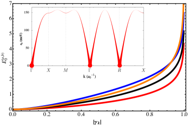
Figure 1: (Color online). The entropy of entanglement $E_{0}^{(a,b)}$ for the two- mode generalized coherent state $|r_{\mathbf{k}},\phi_{\mathbf{k}}\rangle$ (red curve) and for the corresponding first and second excited states as a function of $\left|\gamma_{\mathbf{k}}\right|$. The magnon CV entanglement in the first excited states ($\alpha_{\mathbf{k}}^{\dagger}|r_{\mathbf{k}},\phi_{\mathbf{k}}\rangle$ and $\beta_{\mathbf{k}}^{\dagger}|r_{\mathbf{k}},\phi_{\mathbf{k}}\rangle$) is shown in black. Blue and orange curves illustrate $E_{0}^{(a,b)}$ in the second exited states $(\alpha_{\mathbf{k}}^{\dagger})^{2}|r_{\mathbf{k}},\phi_{\mathbf{k}}\rangle$ (or $(\beta_{\mathbf{k}}^{\dagger})^{2}|r_{\mathbf{k}},\phi_{\mathbf{k}}\rangle$) and $\alpha_{\mathbf{k}}^{\dagger}\beta_{\mathbf{k}}^{\dagger}|r_{\mathbf{k}},\phi_{\mathbf{k}}\rangle$, respectively. The inset depicts magnon dispersion of SrMnO₃ for a selected path of $\mathbf{k}$ along high-symmetry directions of the BZ. The width of the bands depicts the entropy of entanglement.

Although the main focus of our study is on the ground state, we also consider magnon CV entanglement for the two-fold degenerate first excited states $\alpha_{\mathbf{k}}^{\dagger}|r_{\mathbf{k}},\phi_{\mathbf{k}}\rangle$ and $\beta_{\mathbf{k}}^{\dagger}|r_{\mathbf{k}},\phi_{\mathbf{k}}\rangle$, as well as for the three-fold degenerate second excited states $(\alpha_{\mathbf{k}}^{\dagger})^{2}|r_{\mathbf{k}},\phi_{\mathbf{k}}\rangle$, $(\beta_{\mathbf{k}}^{\dagger})^{2}|r_{\mathbf{k}},\phi_{\mathbf{k}}\rangle$, and $\alpha_{\mathbf{k}}^{\dagger}\beta_{\mathbf{k}}^{\dagger}|r_{\mathbf{k}},\phi_{\mathbf{k}}\rangle$. For these states, we find that the entropy of entanglement behaves in a similar way as for the ground state, see Fig. 1, though being slightly larger.

The arithmetic mean of the squared quadrature variances is directly related to the geometry of the spin lattice

$$\Delta(r_{\mathbf{k}},\phi_{\mathbf{k}}) = \frac{1}{2}[\text{Var}^{2}_{r_{\mathbf{k}},\phi_{\mathbf{k}}}(X_{\mathbf{k}}^{A}-X_{\mathbf{k}}^{B})+\text{Var}^{2}_{r_{\mathbf{k}},\phi_{\mathbf{k}}}(P_{\mathbf{k}}^{A}+P_{\mathbf{k}}^{B})]$$ (15)

$$= \cosh 2r_{\mathbf{k}}-\sinh 2r_{\mathbf{k}}\cos\phi_{\mathbf{k}}=\frac{1+\mathrm{Re}[\gamma_{\mathbf{k}}]}{\sqrt{1-|\gamma_{\mathbf{k}}|^{2}}}$$

with $\mathrm{Re}[\gamma_{\mathbf{k}}]$ being the real part of $\gamma_{\mathbf{k}}$. Here, $X_{\mathbf{k}}^{A}(X_{\mathbf{k}}^{B})$ and $P_{\mathbf{k}}^{A}(P_{\mathbf{k}}^{B})$ are the dimensionless position and momentum quadratures of the $a_{\mathbf{k}}(b_{\mathbf{k}})$ mode note1 , and $\text{Var}_{r_{\mathbf{k}},\phi_{\mathbf{k}}}(V)$ is the variance of a given Hermitian operator $V$ with respect to the state $|r_{\mathbf{k}},\phi_{\mathbf{k}}\rangle$.

For $\Delta(r_{\mathbf{k}},\phi_{\mathbf{k}})<1$, which corresponds to $\mathrm{Re}[\gamma_{\mathbf{k}}]<\sqrt{1-|\gamma_{\mathbf{k}}|^{2}}-1$, the two- mode generalized coherent state $|r_{\mathbf{k}},\phi_{\mathbf{k}}\rangle$ is a two- mode squeezed state with mean variance being the associated EPR-uncertainty giedke03 . For $\Delta(r_{\mathbf{k}},\phi_{\mathbf{k}})\geqslant 1$, on the other hand, the EPR-uncertainty is constant and equal to $1$. In the latter case, the amount of nonlocal correlations vanishes giedke03 although the magnon CV entanglement is nontrivial; thus, the magnon CV entanglement can only be related to the EPR-uncertainty in the squeezing domain.

The relation in Eq. (15) allows one to evaluate the CV entanglement in terms of $\Delta(r_{\mathbf{k}},\phi_{\mathbf{k}})$. For real $\gamma_{\mathbf{k}}$, which correspond to $\phi_{\mathbf{k}}=0$ or $\pi$, we find

$$E^{(a,b)}_{0} = \left[\frac{1+\Delta(r_{\mathbf{k}},\phi_{\mathbf{k}})}{2\sqrt{\Delta(r_{\mathbf{k}},\phi_{\mathbf{k}})}}\right]^{2}\log_{2}\left[\frac{1+\Delta(r_{\mathbf{k}},\phi_{\mathbf{k}})}{2\sqrt{\Delta(r_{\mathbf{k}},\phi_{\mathbf{k}})}}\right]^{2}$$ (16)

$$-\left[\frac{1-\Delta(r_{\mathbf{k}},\phi_{\mathbf{k}})}{2\sqrt{\Delta(r_{\mathbf{k}},\phi_{\mathbf{k}})}}\right]^{2}\log_{2}\left[\frac{1-\Delta(r_{\mathbf{k}},\phi_{\mathbf{k}})}{2\sqrt{\Delta(r_{\mathbf{k}},\phi_{\mathbf{k}})}}\right]^{2}.\ \ \ \ \ \$$

The parameter $\Delta(r_{\mathbf{k}},\phi_{\mathbf{k}})$, which depends on the lattice geometry and the choice of $\mathbf{k}$, can be accessed experimentally by detecting coherences of quantum fields, the quadratures, with homodyne detection techniques gross2011 ; peise2015 adapted to a possible magnon-photon coupling yuan2017 ; lachance20 . This may be an avenue forward for experimental detection of the magnon CV entanglement.

In order to further explore the material-specific features of magnon entanglement, we consider a more general spin Hamiltonian, that also has Dzyaloshinskii-Moriya interaction,

$$H=H_{0}+H_{\text{DM}}$$ (17)

with $H_{\text{DM}}=\sum_{\langle ij\rangle}\mathbf{D}_{ij}\cdot\left(\mathbf{S}_{i}\times\mathbf{S}_{j}\right)$ being the DM term with $\mathbf{D}_{ij}=-\mathbf{D}_{ji}$ pointing along the same fixed direction $\mathbf{D}$ for all nearest neighbor spin pairs. By assuming $D=|\mathbf{D}|$, $H$ takes the form

$$H = \sum_{\mathbf{k}}\epsilon_{\mathbf{k}}(\alpha_{\mathbf{k}}^{\dagger}\alpha_{\mathbf{k}}+\beta_{\mathbf{k}}^{\dagger}\beta_{\mathbf{k}})$$ (18)

$$+izDS\sum_{\mathbf{k}}(\gamma_{\mathbf{k}}\alpha_{\mathbf{k}}\beta_{\mathbf{k}}-\gamma_{-\mathbf{k}}\alpha_{\mathbf{k}}^{\dagger}\beta_{\mathbf{k}}^{\dagger}),$$

which is not diagonal anymore in the $(\alpha,\beta)$ modes. Without loss of generality, we assume real-valued $u_{\mathbf{k}}$ in the Bogoliubov transformation of Eq. (9). The second summation of off-diagonal terms on the right hand side implies that there is mixing between $\alpha$ and $\beta$ modes in the presence of the DM interaction. This may cause extra magnon CV entanglement in the ground state of the system. To see this, we diagonalize $H$ by applying another Bogoliubov transformation

$$\left(\begin{array}[]{cc}\alpha_{\mathbf{k}}\\ \beta_{\mathbf{k}}^{\dagger}\end{array}\right)=\left(\begin{array}[]{cc}\eta_{\mathbf{k}}&\zeta_{\mathbf{k}}\\ \zeta^{*}_{\mathbf{k}}&\eta^{*}_{\mathbf{k}}\end{array}\right)\left(\begin{array}[]{cc}\tilde{\alpha}_{\mathbf{k}}\\ \tilde{\beta}_{\mathbf{k}}^{\dagger}\end{array}\right),$$ (25)

where $\zeta_{\mathbf{k}}$ and $\eta_{\mathbf{k}}$ are given by

$$|\eta_{\mathbf{k}}|^{2}=\frac{1}{2\sqrt{1-|\Gamma_{\mathbf{k}}|^{2}}}+\frac{1}{2}, \ \ \ \ |\zeta_{\mathbf{k}}|^{2}=\frac{1}{2\sqrt{1-|\Gamma_{\mathbf{k}}|^{2}}}-\frac{1}{2},$$

$$\frac{\zeta_{\mathbf{k}}}{\eta_{\mathbf{k}}^{*}}=- \frac{1-\sqrt{1-|\Gamma_{\mathbf{k}}|^{2}}}{\Gamma_{\mathbf{k}}},$$ (26)

provided $\Gamma_{\mathbf{k}}=\frac{iD\gamma_{\mathbf{k}}}{J\sqrt{1-|\gamma_{\mathbf{k}}|^{2}}}$ with $|\Gamma_{\mathbf{k}}|<1$. In the $(\tilde{\alpha}_{\mathbf{k}},\tilde{\beta}_{\mathbf{k}}$) modes, the Hamiltonian $H$ takes the diagonal form

$$H = \sum_{\mathbf{k}}\tilde{\epsilon}_{\mathbf{k}}(\tilde{\alpha}_{\mathbf{k}}^{\dagger}\tilde{\alpha}_{\mathbf{k}}+\tilde{\beta}_{\mathbf{k}}^{\dagger}\tilde{\beta}_{\mathbf{k}})$$ (27)

with the dispersion relation ${\epsilon}_{\mathbf{k}}=zS\sqrt{J^{2}(1-|\gamma_{\mathbf{k}}|^{2})-D^{2}|\gamma_{\mathbf{k}}|^{2}}$ (see Supplemental Material for derivation).

The ground state of the diagonal Hamiltonian is a product state $|\psi\rangle=\prod_{\mathbf{k}}|0;\tilde{\alpha}_{\mathbf{k}}\rangle|0;\tilde{\beta}_{\mathbf{k}}\rangle$, where $|0;\tilde{\alpha}_{\mathbf{k}}\rangle$ and $|0;\tilde{\beta}_{\mathbf{k}}\rangle$ are vacuum states of $\tilde{\alpha}_{\mathbf{k}}$ and $\tilde{\beta}_{\mathbf{k}}$, respectively. In this basis, the magnon entanglement is absent. Using the inverse transformation back into the $(\alpha,\beta)$ modes, we express the ground state as

$$|\psi\rangle=\prod_{\mathbf{k}}|\tilde{r}_{\mathbf{k}},\tilde{\phi}_{\mathbf{k}}\rangle$$ (28)

with the entangled two- mode generalized coherent state

$$|\tilde{r}_{\mathbf{k}},\tilde{\phi}_{\mathbf{k}}\rangle=\frac{1}{\cosh\tilde{r}_{\mathbf{k}}}\sum_{n=0}^{\infty}\tanh^{n}\tilde{r}_{\mathbf{k}}e^{in\tilde{\phi}_{\mathbf{k}}}|n;\alpha_{\mathbf{k}}\rangle|n;\beta_{\mathbf{k}}\rangle,$$

(29)

where $|n;\alpha_{\mathbf{k}}\rangle$ and $|n;\beta_{\mathbf{k}}\rangle$ are the $n$th excitation of $\alpha_{\mathbf{k}}$ and $\beta_{\mathbf{k}}$, respectively. Here, $\tilde{r}_{\mathbf{k}}$ and $\tilde{\phi}_{\mathbf{k}}$ are specified by $e^{i\tilde{\phi}_{\mathbf{k}}}\tanh\tilde{r}_{\mathbf{k}}=\frac{\zeta_{\mathbf{k}}}{\eta_{\mathbf{k}}^{*}}$ with $\tilde{r}_{\mathbf{k}}\equiv\tilde{r}_{\mathbf{k}}(\gamma_{\mathbf{k}},\frac{D}{J})\geqslant 0$, and $\tilde{\phi}_{\mathbf{k}}\equiv\tilde{\phi}_{\mathbf{k}}(\gamma_{\mathbf{k}},\frac{D}{J})=\pi-\arg[\Gamma_{\mathbf{k}}]=\frac{\pi}{2}-\arg[\gamma_{\mathbf{k}}]$. In the case of $D=0$, the only relevant term is $n=0$, i.e., $|\tilde{r}_{\mathbf{k}},\tilde{\phi}_{\mathbf{k}}\rangle=|0;\alpha_{\mathbf{k}}\rangle|0;\beta_{\mathbf{k}}\rangle$ and thus $|\psi\rangle=|\psi_{0}\rangle$. The entropy of entanglement in the $(\alpha,\beta)$ modes

$$E^{(\alpha,\beta)}=|\eta_{\mathbf{k}}|^{2}\log_{2}|\eta_{\mathbf{k}}|^{2}-|\xi_{\mathbf{k}}|^{2}\log_{2}|\xi_{\mathbf{k}}|^{2},$$ (30)

is a function of $\left|\gamma_{\mathbf{k}}\right|$ and the relative coupling strength $\frac{D}{J}$. Fig. 2 shows magnon CV entanglement $E^{(\alpha,\beta)}$ as a function of $\left|\gamma_{\mathbf{k}}\right|$ for selected values of $\frac{D}{J}$.

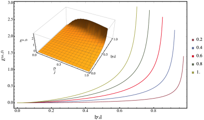
Figure 2: (Color online). The entropy of entanglement $E^{(\alpha,\beta)}$ of the two- mode generalized coherent state $|\tilde{r}_{\mathbf{k}},\tilde{\phi}_{\mathbf{k}}\rangle$ as a function of $\left|\gamma_{\mathbf{k}}\right|$ and $\frac{D}{J}$ in the $(\alpha,\beta)$ modes. In the main figure, we show plots for different values of $\frac{D}{J}$, while the inset is a three-dimensional plot of the entropy of entanglement as a function of $\frac{D}{J}$ and $\left|\gamma_{\mathbf{k}}\right|$.

In the $(\alpha,\beta)$ modes, the two-mode magnon entanglement, Eq. (30), is non-trivial, while, as shown above, the symmetric Heisenberg interaction $H_{0}$ on its own does not generate any magnon entanglement in these modes, i.e., $E^{(\alpha,\beta)}_{0}=0$. Thus, the antisymmetric DM interaction is mainly responsible for the entanglement contribution in Eq. (30), and we identify $E^{(\alpha,\beta)}_{\text{DM}}=E^{(\alpha,\beta)}$ as the DM-induced entanglement.

To have a clearer picture of the hierarchy of the magnon CV entanglement, we transform the ground state $|\psi\rangle$ back into the original $(a,b)$ modes

$$|\psi\rangle=\prod_{\mathbf{k}}|\hat{r}_{\mathbf{k}},\hat{\phi}_{\mathbf{k}}\rangle,$$ (31)

with the two- mode generalized coherent state

$$|\hat{r}_{\mathbf{k}},\hat{\phi}_{\mathbf{k}}\rangle=\frac{1}{\cosh\hat{r}_{\mathbf{k}}}\sum_{n=0}^{\infty}\tanh^{n}\hat{r}_{\mathbf{k}}e^{in\hat{\phi}_{\mathbf{k}}}|n;a_{\mathbf{k}}\rangle|n;b_{\mathbf{k}}\rangle,\ \ \ \ \ \$$ (32)

where $e^{i\hat{\phi}_{\mathbf{k}}}\tanh\hat{r}_{\mathbf{k}}=\frac{v_{\mathbf{k}}\eta^{*}_{\mathbf{k}}+u_{\mathbf{k}}\zeta_{\mathbf{k}}}{u^{*}_{\mathbf{k}}\eta^{*}_{\mathbf{k}}+v^{*}_{\mathbf{k}}\zeta_{\mathbf{k}}}$, $\hat{r}_{\mathbf{k}}\equiv\hat{r}_{\mathbf{k}}(\gamma_{\mathbf{k}},\frac{D}{J})\geqslant 0$, and $\hat{\phi}_{\mathbf{k}}\equiv\hat{\phi}_{\mathbf{k}}(\gamma_{\mathbf{k}},\frac{D}{J})=\pi-\arg[\gamma_{\mathbf{k}}(1+i\frac{D}{J})]$. The total entropy of entanglement in the $(a,b)$ modes for this state is

$$E^{(a,b)} = \cosh^{2}\hat{r}_{\mathbf{k}}\log_{2}[\cosh^{2}\hat{r}_{\mathbf{k}}]-\sinh^{2}\hat{r}_{\mathbf{k}}\log_{2}[\sinh^{2}\hat{r}_{\mathbf{k}}].\ \ \ \ \ \ \$$ (33)

Figure 3 shows the entanglement of Eq. (33) as function of $\left|\gamma_{\mathbf{k}}\right|$, for selected values of $\frac{D}{J}$. Note that increasing values of the DM interaction leads to an enhancement of the entanglement for all $\left|\gamma_{\mathbf{k}}\right|$.

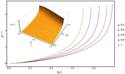
Figure 3: (Color online). The entropy of entanglement of the two- mode generalized coherent state $|\hat{r}_{\mathbf{k}},\hat{\phi}_{\mathbf{k}}\rangle$ as a function of $\left|\gamma_{\mathbf{k}}\right|$ and the relative coupling strength $\frac{D}{J}$ in the $(a,b)$ modes. In the main figure, we show several sections of this function for different values of $\frac{D}{J}$, and the inset is a full three-dimensional plot.

Since $E^{(a,b)}|_{D=0}=E_{0}^{(a,b)}$, we may write

$$E^{(a,b)}=E_{0}^{(a,b)}+E^{(a,b)}_{\text{DM}},$$ (34)

where $E^{(a,b)}_{\text{DM}}$ vanishes in the absence of DM interaction, and we refer to it as the DM-induced entanglement in the $(a,b)$ modes. Unlike the $(\alpha,\beta)$ modes, in the $(a,b)$ modes both the Heisenberg and the DM interactions induce non-zero contributions to the magnon entanglement in the ground state.

The magnon CV entanglement is an intrinsic property of antiferromagnets that depends on the geometry of the spin lattice as encoded in $\gamma_{\mathbf{k}}$ and on the relative coupling strength $\frac{D}{J}$. Both parameters are material-dependent and can vary strongly from system to system. This opens an interesting route to search for suitable entanglement hosts among the existing thousands of magnetic compounds, and poses a natural question of how magnon entanglement can be detected in an experiment. Similar to what was discussed above in the pure Heisenberg case, the magnon CV entanglement in the presence of DM interaction can be measured experimentally by detecting quadratures corresponding to the arithmetic mean variance $\Delta(\hat{r}_{\mathbf{k}},\hat{\phi}_{\mathbf{k}})$ in a homodyne detection setup gross2011 ; peise2015 adapted to a possible magnon-photon coupling yuan2017 ; lachance20 . In the $(a,b)$ modes, one may extract the parameter $\hat{r}_{\mathbf{k}}$ from

$$\Delta(\hat{r}_{\mathbf{k}},\hat{\phi}_{\mathbf{k}})=\cosh 2\hat{r}_{\mathbf{k}}-\sinh 2\hat{r}_{\mathbf{k}}\cos\hat{\phi}_{\mathbf{k}}$$ (35)

to evaluate the total entanglement $E^{(a,b)}$ in Eq. (33). Here, we used Eq. (15) replacing the state $|r_{\mathbf{k}},\phi_{\mathbf{k}}\rangle$ by the state $|\hat{r}_{\mathbf{k}},\hat{\phi}_{\mathbf{k}}\rangle$. In the domain of $\tanh\hat{r}_{\mathbf{k}}\leqslant\cos\hat{\phi}_{\mathbf{k}}$ corresponding to $\mathrm{Re}[\gamma_{\mathbf{k}}(J+iD)]<\sqrt{J^{2}(1-|\gamma_{\mathbf{k}}|^{2})-|\gamma_{\mathbf{k}}|^{2}D^{2}}-J$, the two- mode generalized coherent state $|\hat{r}_{\mathbf{k}},\hat{\phi}_{\mathbf{k}}\rangle$ is also a two- mode squeezed state, and the mean variance $\Delta(\hat{r}_{\mathbf{k}},\hat{\phi}_{\mathbf{k}})$ is the associated EPR-uncertainty giedke03 .

We conclude with some final remarks. In the analysis of different bosonic modes, we notice different types of two-mode magnon entanglement residing in the ground state. In Fig. 4, we compare entropies of entanglement for an antiferromagnet with a simple cubic crystal structure, where the Hamiltonian is effectively described by nearest neighbor Heisenberg exchange as well as DM interaction with typical ratio $D/J\approx 30\%$ meyer2017 ; chern2006 ; zakeri2017 . It can be seen that from $(a,b)$ modes to $(\alpha,\beta)$ modes the Heisenberg contribution to entanglement decreases while the DM-induced magnon CV entanglement increases. This is due to the fact that different bosonic modes represent different tensor product structures of the Hilbert space zanardi2004 . While the $(a,b)$ modes describe naturally identifiable magnon modes, being associated with each sublattice, the $(\alpha,\beta)$ and $(\tilde{\alpha},\tilde{\beta})$ modes are hybridized and their number states are described by superpositions of excitations in the $(a,b)$ modes. Although the stronger entanglement, a feature particularly useful in quantum information science and technology, is available in the $(a,b)$ modes, the usefulness of these modes in an actual experiment must be determined by a suitable tensor product decomposition.

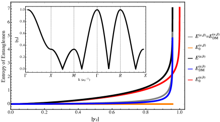
Figure 4: (Color online). Hierarchy of magnon entanglement for an antiferromagnet as a function of $\left|\gamma_{\mathbf{k}}\right|$. Definition of the different entanglement entropies is given in the main text. An effective DM interaction with the strength of $30\%$ of the Heisenberg exchange $J$ is used. The inset illustrates the dependence of entanglement on $\mathbf{k}$ in a simple cubic crystal structure.

The condition for diagonalizing the Hamiltonians in terms of bosonic operators is that $|\gamma_{\mathbf{k}}|<1$ in the pure Heisenberg case and $|\gamma_{\mathbf{k}}|^{2}<\frac{J^{2}}{J^{2}+D^{2}}$ in the presence of DM interaction. Since ${D}$ is typically less than a few tenths of ${J}$ for most materials meyer2017 ; chern2006 ; zakeri2017 , this condition is not satisfied only for a very small part of the BZ, e.g., the region around zone center. We would like to remark that the entire BZ may be included in this analysis by considering a Hamiltonian that possesses single ion uniaxial anisotropy, $-\mathcal{K}({\bf n}\cdot{\bf S})^{2}$, e.g., with easy-axis ${\bf n}$ along the direction of the DM vector, as long as $|1+\frac{2\mathcal{K}}{zJ}|>\sqrt{1+\frac{D^{2}}{J^{2}}}$. Note that any change of symmetry in the Hamiltonian introduces new magnon modes and hence new levels of entanglement contribution in the hierarchy of two-mode magnon entanglement. Our general message is not changed by this, although the technical level of calculations may become more intricate. It is interesting to note that already very mild uniaxial anisotropy of $0.001\%$ of $J$ along $z$ axis, when included in a pure Heisenberg Hamiltonian ($D=0$), allows to regularize the magnon CV entanglement dependence on $|\gamma_{\bf k}|$. At $|\gamma_{\bf k}|=1$, we obtain $E_{0}^{(a,b)}\approx 9.04$. In a more generic case of Heisenberg-DMI with $D/J=0.1$, $z=6$ and uniaxial anisotropy of $\mathcal{K}/J=$0.015 along $\mathbf{D}$, we find $E^{(a,b)}\approx 8.094$ and $E^{(\alpha,\beta)}\approx 4.766$ at $|\gamma_{\bf k}|=1$.

In contrast to Ref. bossini2019 , where photoinduced spin dynamics was employed to trigger entanglement between a pair of magnon modes, our analysis shows that ground state two-mode magnon entanglement in antiferromagnets is an intrinsic property of the magnetic structure that is already given by the geometry of the spin lattice and exchange couplings, which should be accessible to experimental detection. We have examined the magnon entanglement in quantum magnetic structures with nearest neighbor antiferromagnetic Heisenberg exchange and DM interaction. The analysis is appropriate for many classes of compounds, but we would like to mention in particular the transition metal oxides that have a vast crystallographic phase space, which allows both for tunability of $\frac{D}{J}$ as well as $\gamma_{\mathbf{k}}$. A concrete example that is known to exhibit only nearest neighbor Heisenberg exchange is SrMnO₃ zhu2020 . We also note that materials like La₂CuO₄ voigt1996 , FeBO₃, and CoCO₃ beutier2017 are well studied antiferromagnets that are known to have DM interaction in the here studied range of $\frac{D}{J}$.

References

(1) A. Einstein, B. Podolsky, and N. Rosen,
Can Quantum-Mechanical Description of Physical Reality Be Considered Complete?,
Phys. Rev. 47, 777 (1935).
(2) Z. Y. Ou, S. F. Pereira, H. J. Kimble, and K. C. Peng,
Realization of the Einstein-Podolsky-Rosen paradox for continuous variables,
Phys. Rev. Lett. 68, 3663 (1992).
(3) G. Giedke, M. M. Wolf, O. Krüger, R. F. Werner, and J. I. Cirac,
Entanglement of Formation for Symmetric Gaussian States,
Phys. Rev. Lett. 91, 107901 (2003).
(4) M. D. Reid, P. D. Drummond, W. P. Bowen, E. G. Cavalcanti,
P. K. Lam, H. A. Bachor, U. L. Andersen, and G. Leuchs,
The Einstein-Podolsky-Rosen paradox: From concepts to applications,
Rev. Mod. Phys. 81, 1727 (2009).
(5) S. L. Braunstein and P. van Loock,
Quantum information with continuous variables,
Rev. Mod. Phys. 77, 513 (2005).
(6) S. L. Braunstein and H. J. Kimble,
Teleportation of Continuous Quantum Variables,
Phys. Rev. Lett. 80, 869 (1998).
(7) T. Opatrný and G. Kurizki,
Matter-Wave Entanglement and Teleportation by Molecular Dissociation and Collisions,
Phys. Rev. Lett. 86, 3180 (2001).
(8) K. Hammerer, A. S. Sørensen, and E. S. Polzik,
Quantum interface between light and atomic ensembles,
Rev. Mod. Phys. 82, 1041 (2010).
(9) V. Giovannetti, S. Lloyd, and L. Maccone,
Quantum-enhanced measurements: beating the standard quantum limit,
Science 306, 1330 (2004).
(10) P. Mohn,
Magnetism in the Solid State: an Introduction
(Springer-Verlag, Berlin, 2006).
(11) J. Googenough,
Localized to Itinerant Electronic Transition in Perovskite Oxides
(Springer-Verlag, Berlin, 2020).
(12) Entropy of entanglement of a pure bipartite state
is defined as the von Neumann entropy of the reduced density operator
of one of the two subsystems or . Explicitly, given the Schmidt form
, one
has .
(13) X. Zhu, A. Edström, and C. Ederer,
Magnetic exchange interactions in SrMnO3,
Phys. Rev. B 101, 064401 (2020).
(14) Dimensionless position and momentum quadratures of the
and modes are ,
,
,
and .
(15) C. Gross, H. Strobel, E. Nicklas, T. Zibold, N. Bar-Gill, G. Kurizki,
and M. K. Oberthaler,
Atomic homodyne detection of continuous-variable entangled twin-atom states,
Nature 480, 219 (2011).
(16) J. Peise, I. Kruse, K. Lange, B. Lücke, L. Pezzè, J. Arlt, W. Ertmer,
K. Hammerer, L. Santos, A. Smerzi, and C. Klempt,
Satisfying the Einstein- Podolsky- Rosen criterion with massive particles,
Nature Comm. 6, 8984 (2015).
(17) H. Y. Yuan and X. R. Wang,
Magnon-photon coupling in antiferromagnets,
Appl. Phys. Lett. 110, 082403 (2017).
(18) D. Lachance-Quirion, S. P. Wolski, Y. Tabuchi, S. Kono, K. Usami, and
Y. Nakamura,
Entanglement-based single-shot detection of a single magnon with a superconducting qubit,
Science 367, 425 (2020).
(19) S. Meyer, B. Dupé, P. Ferriani, and S. Heinze
Dzyaloshinskii-Moriya interaction at an antiferromagnetic interface: First-principles study
of Fe/Ir bilayers on Rh(001),
Phys. Rev. B 96, 094408 (2017).
(20) G.-W. Chern, C. J. Fennie, and O. Tchernyshyov,
Broken parity and a chiral ground state in the frustrated magnet
CdCr2O4,
Phys. Rev. B 74, 060405(R) (2006).
(21) K. Zakeri,
Probing of the interfacial Heisenberg and Dzyaloshinskii- Moriya exchange interaction by
magnon spectroscopy,
J. Phys.: Condens. Matter 29, 013001 (2017).
(22) P. Zanardi, D. A. Lidar and S. Lloyd,
Quantum Tensor Product Structures are Observable Induced,
Phys. Rev. Lett. 92, 060402 (2004).
(23) D. Bossini, S. Dal Conte, G. Cerullo, O. Gomonay, R. V. Pisarev,
M. Borovsak, D. Mihailovic, J. Sinova, J. H. Mentink, Th. Rasing, and A. V. Kimel,
Laser-driven quantum magnonics and terahertz dynamics of the order parameter in antiferromagnets,
Phys. Rev. B 100, 024428 (2019).
(24) A. Voigt and J. Richter,
The - antiferromagnet on the square lattice with Dzyaloshinskii - Moriya interaction:
an exact diagonalization study,
J. Phys.: Condens. Matter 8, 5059 (1996).
(25) G. Beutier, S. P. Collins, O. V. Dimitrova, V. E. Dmitrienko,
M. I. Katsnelson, Y. O. Kvashnin, A. I. Lichtenstein, V. V. Mazurenko, A. G. A. Nisbet,
E. N. Ovchinnikova, and D. Pincini,
Band Filling Control of the Dzyaloshinskii-Moriya Interaction in Weakly Ferromagnetic Insulators,
Phys. Rev. Lett. 119, 167201 (2017).