Phase space theory for open quantum systems with local and collective dissipative processes

Abstract

In this article we investigate driven dissipative quantum dynamics of an ensemble of two-level systems given by a Markovian master equation with collective and non-collective dissipators. Exploiting the permutation symmetry in our model, we employ a phase space approach for the solution of this equation in terms of a diagonal representation with respect to certain generalized spin coherent states. Remarkably, this allows to interpolate between mean-field theory and finite system size in a formalism independent of Hilbert-space dimension. Moreover, in certain parameter regimes, the evolution equation for the corresponding quasiprobability distribution resembles a Fokker-Planck equation, which can be efficiently solved by stochastic calculus. Then, the dynamics can be seen as classical in the sense that no entanglement between the two-level systems is generated. Our results expose, utilize and promote techniques pioneered in the context of laser theory, which we now apply to problems of current theoretical and experimental interest.

I Introduction

Quantum optical models, such as the Dicke model, where an ensemble of identical two-level atoms is coupled to a cavity mode, have been among the first systems where emergent collective behavior such as super-radiance has been investigated Dicke (1954). The cooperative effects can be described in terms of collective atomic operators in such a way that the ensemble of $N$ two-level atoms is treated as a large spin of length $j=\frac{N}{2}$. Interestingly, such a cooperative state can still possess non-trivial quantum correlations Dicke (1954). The proposal on how to implement the Dicke model in an optical cavity QED system Dimer et al. (2007) and the experimental realization using a super-fluid gas trapped inside an optical cavity Baumann et al. (2010) are important milestones, which have inspired more studies on the role of collective effects in quantum phase transitions, such as Nataf et al. (2019); Johnson et al. (2019).

Purely collective dynamics cannot always be achieved due to experimental conditions, for example when the ensemble of two level systems is inhomogeneous Lalumière et al. (2013) or when the individual two level systems couple to different reservoirs Galve et al. (2017). In these cases, the dimensionality of the relevant Hilbert space in general grows exponentially with the system size. An interesting alternative regime exists when in addition to collective processes only local processes occur which preserve permutation invariance. This holds if all non-collective processes are identical for each constituent in the ensemble. In this regime, permutation invariance can be utilized to reduce the effective dimension of the problem Shammah et al. (2018). Formally, this can be understood as follows. In an ensemble of $N$ two-level systems, collective processes confine the dynamics on a subspace $\mathcal{H}_{j}\subset\mathbb{C}^{2N}$ spanned by the Dicke states $\ket{j,m}$, where $-j\leq m\leq j$, whereas the permutation invariant local processes couple the different subspaces $\mathcal{H}_{j^{\prime}}$ spanned by Dicke ladders labeled by differing $j^{\prime}$. The reduction in the effective dimension emerges due to high degeneracy of the Dicke states Mandel and Wolf (1995).

When local and collective processes coexist, a host of interesting phenomena can be studied. For example, incoherent pumping on a super-radiant ensemble of two level systems can lead to robust steady state super-radiance Meiser and Holland (2010). Competing collective phenomena, such as driving and dissipation can lead to non-equilibrium phase transitions Iemini et al. (2018); Link et al. (2019) and recently the robustness of such transitions against local dephasing has been investigated Tucker et al. (2018).

In this article we will investigate a paradigmatic driven, dissipative open system consisting of $N$ two level atoms which is affected by both collective and permutation invariant local dissipative processes. We describe the dynamics of such a system with the following GKSL type master equation Gorini et al. (1976); Lindblad (1976)

$$\partial_{t}\rho=\mathcal{L}[\rho]=-i[H,\rho]+\mathcal{L}_{l}[\rho]+\mathcal{L}_{c}[\rho]\,,$$ (1)

where collective driving is given by

$$H=\sum_{\lambda=1}^{N}\frac{1}{2}\vec{B}\cdot\vec{\sigma}_{\lambda}\equiv\vec{B}\cdot\vec{J}\,,$$ (2)

with $\vec{B}\in^{3}$, $\sigma_{\lambda}^{i}=\sigma_{i}$ for $i=z,\pm$ are Pauli spin matrices $\sigma_{z}$, $\sigma_{\pm}=\sigma_{x}\pm i\sigma_{y}$ acting on system $\lambda$, and $\vec{J}$ is the collective spin operator with components $J_{z}$ and $J_{\pm}=J_{x}\pm iJ_{y}$. The collective dissipation is given by

$$\mathcal{L}_{c}[\rho]=\sum_{k=z,\pm}\mathcal{L}_{c}^{k}[\rho]=\sum_{k=z,\pm}\frac{2\kappa_{k}}{N}\left(J_{k}\rho J_{k}^{\dagger}-\frac{1}{2}\left\{J_{k}^{\dagger}J_{k},\rho\right\}\right)\,,$$ (3)

whereas the permutation invariant local dissipation is given by

$$\mathcal{L}_{s}[\rho]=\sum_{k=z,\pm}\sum_{\lambda=1}^{N}\frac{\gamma_{k}}{2}\left(\sigma_{\lambda}^{k}\rho\sigma_{\lambda}^{k\dagger}-\frac{1}{2}\left\{\sigma_{\lambda}^{k\dagger}\sigma_{\lambda}^{k},\rho\right\}\right)\,.$$ (4)

We assume that all of the local and collective rates, $\gamma_{k}$ and $\kappa_{k}$ respectively, are non-negative, so that the dynamics generated by the master equation is completely positive. Note that the non-collective term does not commute with the total angular momentum $\vec{J}^{2}$. It therefore couples different eigenspaces of $\vec{J}^{2}$ in contrast to the collective terms.

Instead of using the basis of Dicke states directly, we will employ a phase space approach by representing the state of the open system in terms of generalized spin coherent states and the associated $P$-function Gisin and Cibils (1992); Puri and Lawande (1980). This type of approach to collective phenomena has been already discussed in the quantum optics community during the 70s and 80s of the previous century, in the context of cooperative fluorescence Walls et al. (1978); Walls (1980); Drummond and Carmichael (1978); Carmichael (1980). The generalized coherent state approach that we take has been pioneered in Weidlich et al. (1967a, b); Haken et al. (1967) and used also more recently in Patra et al. (2019). Here we show that in certain parameter regions this method can be used to map the solution of master equation (1) to a Fokker-Planck equation for any system size. Then the dynamics is classical in the sense that no quantum correlations between the two-level systems build up. In the method the system size is merely a parameter determining the strength of diffusion in phase space. Therefore, it allows to analytically interpolate between finite-size and mean-field theory.

The outline of the article is the following. First we introduce a generalization of spin coherent states in section II. In section III we derive the equation of motion for the associated $P$-function. The phase space approach provides immediately a consistent mean field theory, which we explore in section IV. In section V we focus on the exact semi-classical regime of our model, where the equations of motion can be efficiently solved. At last, we conclude with discussion and outlook in section VI.

II Generalized Spin Coherent States

The main technical tool of this paper is to expand the state of all identical two level systems in terms of a generalized $P$-representation. More precicely, consider the density operator $\alpha(\vec{r})$ of the simplest product state where all two level systems are identical

$$\alpha(\vec{r})=\bigotimes\limits_{\lambda=1}^{N}\frac{1}{2}(\mathbbm{1}+\vec{\sigma}\cdot\vec{r})\,.$$ (5)

This state is positive iff the Bloch vector $\vec{r}$ has a length smaller or equal to 1. It is pure iff $|\vec{r}|^{2}=1$. We show later on that in this case the definition (5) reduces to the standard spin coherent states in the symmetric Dicke subspace with $j=\frac{N}{2}$. Due to this property, we call these states the generalized coherent states. However, we stress that these are not pure states and do not have the same group theoretical interpretation as regular coherent states Zhang et al. (1990). We will later express the state in terms of a diagonal representation using a $P$-function associated with these generalized coherent states. Firstly, let us discuss how certain operators act on these states. A direct calculation shows that

$$\sigma_{k}(\mathbbm{1}+\vec{\sigma}\cdot\vec{r})=\big{[}r_{k}+(\delta_{ki}-\mathrm{i}\varepsilon_{kij}r_{j}-r_{k}r_{i})\partial_{i}\big{]}(\mathbbm{1}+\vec{\sigma}\cdot\vec{r})\,,$$ (6)

$$(\mathbbm{1}+\vec{\sigma}\cdot\vec{r})\sigma_{k}=\big{[}r_{k}+(\delta_{ki}+\mathrm{i}\varepsilon_{kij}r_{j}-r_{k}r_{i})\partial_{i}\big{]}(\mathbbm{1}+\vec{\sigma}\cdot\vec{r})\,,$$ (7)

where the derivatives are with respect to $\vec{r}$, i.e. $\partial_{i}=\partial/\partial r_{i}$, and summation over repeated indices is implied. With these relations we can replace the action of operators acting on generalized coherent states by differential operators. One example is the total angular momentum operator $\vec{J}$

$$\begin{split}J_{k}\alpha(\vec{r})&=\frac{1}{2}\sum_{\lambda=1}^{N}\frac{1}{2}(\mathbbm{1}+\vec{\sigma}\cdot\vec{r})\otimes...\otimes\underbrace{\sigma_{k}\frac{1}{2}(\mathbbm{1}+\vec{\sigma}\cdot\vec{r})}_{\text{$\lambda$'th position}}\otimes...\otimes\frac{1}{2}(\mathbbm{1}+\vec{\sigma}\cdot\vec{r})=\text{(use product rule)}\\ &=\frac{N}{2}r_{k}\alpha(\vec{r})+\frac{1}{2}(\delta_{ki}-\mathrm{i}\varepsilon_{kij}r_{j}-r_{k}r_{i})\partial_{i}\alpha(\vec{r})\,.\end{split}$$ (8)

This gives us the algebra of spin coherent states. It is analogous to well known relations such as $a\ket{z}=z\ket{z}$ in the case of bosons. With these rules we can express the action of the Hamiltonian part, as well as the collective dissipative part of the Lindbladian (1), onto a coherent state as a differential operator with respect to the coherent state label $\vec{r}$. Due to our more general definition of spin coherent states, this is also true for the local dissipators. Consider for instance identical local dephasing (in the $\sigma_{z}$ basis with rate $\gamma_{z}/2$) of all two level systems

$$\begin{split}\mathcal{L}_{s}^{z}[\alpha(\vec{r})]=\frac{\gamma_{z}}{2}\sum_{\lambda}\mathcal{L}_{s,\lambda}^{z}[\alpha(\vec{r})]=\frac{\gamma_{z}}{2}\sum_{\lambda=1}^{N}\frac{1}{2}(\mathbbm{1}+\vec{\sigma}\cdot\vec{r})\otimes...\otimes\underbrace{\mathcal{L}_{\lambda}^{z}[\frac{1}{2}(\mathbbm{1}+\vec{\sigma}\cdot\vec{r})]}_{\text{$\lambda$'th position}}\otimes...\otimes\frac{1}{2}(\mathbbm{1}+\vec{\sigma}\cdot\vec{r})\,.\end{split}$$ (9)

Now the action of any superoperator on a two level system can always be written as a first order differential operator with respect to the Bloch vector. This is obvious because the state itself is linear in $\vec{r}$. In the example of dephasing we find

$$\mathcal{L}_{\lambda}^{z}[\frac{1}{2}(\mathbbm{1}+\vec{\sigma}\cdot\vec{r})]=\sigma_{z}\frac{1}{2}(\mathbbm{1}+\vec{\sigma}\cdot\vec{r})\sigma_{z}-\{\sigma_{z}^{2},\frac{1}{4}(\mathbbm{1}+\vec{\sigma}\cdot\vec{r})\}=(-2x\partial_{x}-2y\partial_{y})\frac{1}{2}(\mathbbm{1}+\vec{\sigma}\cdot\vec{r})\,.$$ (10)

with canonical notation $r_{1}=x,\,r_{2}=y,\,r_{3}=z$. Inserting this in the above expression and using the product rule one finds for the coherent state

$$\begin{split}\mathcal{L}_{s}^{z}[\alpha(\vec{r})]=(-{\gamma_{z}}x\partial_{x}-{\gamma_{z}}y\partial_{y})\alpha(\vec{r})\,.\end{split}$$ (11)

Of course, the same calculations can be done for local decay and pump channels. In summary, we can now express the action of the entire Lindblad superoperator on a generalized spin coherent state as a differential operator with respect to the state label, that is the vector $\vec{r}$.
Let us briefly make the connection to the standard spin coherent states. These are usually defined in an eigenspace of $\vec{J}^{2}$ with eigenvalue $j=\frac{N}{2}$ (symmetric Dicke states). They are rotations of the ’fully polarized’ state $\alpha(\vec{e}_{z})$. We recover these states from our generalized coherent states by setting $|\vec{r}|=r=1$. For better illustration, let us parameterize the vector with spherical coordinates

$$\vec{r}=\begin{pmatrix}r\sqrt{1-\eta^{2}}\cos\phi\\ r\sqrt{1-\eta^{2}}\sin\phi\\ r\eta\end{pmatrix}\,,\qquad\phi\in[0,2\pi)\,,\qquad\eta\in[-1,1]\,,\qquad r\in[0,1]\,,$$ (12)

where one may identify $\eta=\cos\theta$. The differential representation of the dissipators in these coordinates are provided in appendix B. The main insight is that for $r=1$ in the collective operators, no derivatives with respect to $r$ appear. The radius is preserved because the dynamics does not lead out of the symmetric $j=N/2$ subspace. This is different in the case of local dissipation. The local dissipators are not confined to this subspace which is reflected in the occurence of derivatives with respect to $r$. If the dynamics remains in the Dicke subspace however, the equations of motions which we derive in the next section will automatically conserve $r=1$ so that both cases are covered in the formalism. Now as an ansatz we express the state with a diagonal representation in terms of the generalized coherent states

$$\rho=\int\limits_{r\leq 1}d^{3}r\,P(\vec{r})\,\alpha(\vec{r})\,,$$ (13)

with a generalized $P$-function $P(\vec{r})$, which is a quasiprobability distribution on the unit ball in ³ centered at the origin. As $\alpha(\vec{r})$ is a polynomial in $\vec{r}$ of order $N$, it is obvious that $P$ is not unique. If $\rho$ is a normalized state, the distribution is normalized as well

$$1=\text{tr}\left\{\rho\right\}=\int\limits_{r\leq 1}d^{3}r\,P(\vec{r})\,\text{tr}\left\{\alpha(\vec{r})\right\}=\int\limits_{r\leq 1}d^{3}r\,P(\vec{r})\,.$$ (14)

If $P(\vec{r})$ is a positive function, the state is also positive by construction. However, $P(\vec{r})$ does not need to be positive. In fact, if $P(\vec{r})$ is positive for all $\vec{r}$, then the state is separable by definition, as it is a classical mixture of separable states. An entangled state necessarily has a negative $P$ function. Once the $P$ function of the state is known, all observables can be computed easily

$$\text{tr}\left\{\rho O\right\}=\int\limits_{r\leq 1}d^{3}r\,P(\vec{r})\,\text{tr}\left\{\alpha(\vec{r})O\right\}\,.$$ (15)

For example, in the case of the angular momentum operator one finds $\text{tr}\left\{\alpha(\vec{r})\vec{J}\right\}=N/2\vec{r}$ so that

$$\text{tr}\left\{\rho\vec{J}\right\}=\frac{N}{2}\int\limits_{r\leq 1}d^{3}r\,P(\vec{r})\,\vec{r}\,.$$ (16)

III Equation of motion for the P-function

With the differential form of operators at hand, it is a straightforward task to derive an equation of motion for the $P$-function of a state evolving under the GKSL equation (1). One simply plugs in the expression (13) in the equation of motion

$$\begin{split}\partial_{t}\rho&=\int\limits_{r\leq 1}d^{3}r\,\partial_{t}P(\vec{r})\,\alpha(\vec{r})=\mathcal{L}[\rho]=\int\limits_{r\leq 1}d^{3}r\,P(\vec{r})\,\mathcal{L}[\alpha(\vec{r})]\,.\end{split}$$ (17)

Using the differential representation, we can express the action of the GKSL-generator as a second order differential operator

$$\mathcal{L}[\alpha(\vec{r})]=\Big{(}a_{i}(\vec{r})\partial_{i}+\frac{1}{2N}D_{ij}(\vec{r})\partial_{i}\partial_{j}\Big{)}\alpha(\vec{r})\,.$$ (18)

To find the “forward in time” equation of motion for $P$ one performs partial integration under the integral, neglecting boundary terms. Comparison of the integrands on the left and right hand sides gives the following partial differential equation

$$\partial_{t}P(\vec{r})=\Big{(}-\partial_{i}a_{i}(\vec{r})+\frac{1}{2N}\partial_{i}\partial_{j}D_{ij}(\vec{r})\Big{)}P(\vec{r})\,.$$ (19)

General expressions for $\vec{a}(\vec{r})$ and $D(\vec{r})$ are provided in appendix A. This exact equation has the form of a second order Kramers-Moyal expansion. However, we point out that the matrix $D(\vec{r})$ is in general not positive for all $\vec{r}$. When $D(\vec{r})$ is positive semidefinite for all $\vec{r}$, the equation corresponds to a Fokker-Planck equation. Since the Fokker-Planck equation always preserves the positivity, it is clear that the diffusion can be positive only if the dynamics does not generate entanglement between the two level systems. Indeed, we do find certain parameter regimes in our model where this holds true. Then the partial differential equation is well behaved and can easily be integrated numerically using stochastic differential equations. We give a detailed description of this in section V.

IV Mean field theory

From equation (19) follows directly a ’mean field’ approximation by neglecting the diffusion term. In general, this approximation is exact in the thermodynamical limit $N\rightarrow\infty$ because then the diffusion vanishes exactly due to the prefactor $\frac{1}{N}$. The remaining equation of motion is first order and can be solved by the method of characteristics

$$\partial_{t}P(\vec{r})=-\partial_{i}a_{i}(\vec{r})P(\vec{r})\,.$$ (20)

The solution is given by the time evolution of the initial distribution along the mean-field trajectories

$$P_{t}(\vec{r})=\int{\rm d}^{3}r_{0}P_{0}(\vec{r}_{0})\delta(\vec{r}-\vec{r}(t))\,,\qquad\vec{r}(0)=\vec{r}_{0}\,,\qquad\dot{\vec{r}}(t)=\vec{a}(\vec{r}(t))\,.$$ (21)

If the system starts in a coherent state, i.e. $\rho_{0}=\alpha(\vec{r}_{0})$ or $P_{0}(\vec{r})=\delta(\vec{r}-\vec{r}_{0})$, then the state remains a coherent state under mean field evolution and $\rho_{t}=\alpha(\vec{r}(t))$ or $P_{t}(\vec{r})=\delta(\vec{r}-\vec{r}(t))$. For our master equation the mean field equations of motion are explicitly

$$\begin{split}&\dot{x}={B_{y}}z-{B_{z}}y+x(\gamma_{-}-\gamma_{+}-\gamma_{z}+\kappa_{-}z-\kappa_{+}z)\,,\\ &\dot{y}=-{B_{x}}z+{B_{z}}x+y(\gamma_{-}-\gamma_{+}-\gamma_{z}+\kappa_{-}z-\kappa_{+}z)\,,\\ &\dot{z}={B_{x}}y-{B_{y}}x-(\kappa_{-}-\kappa_{+})\left(x^{2}+y^{2}\right)+2\gamma_{-}(z-1)-2\gamma_{+}(z+1)\,,\end{split}$$ (22)

where we have neglected subleading terms of order $1/N$ consistent with neglection of the diffusion. Note that collective dephasing does not influence the mean field dynamics. Except for some fine tuned cases Link et al. (2019); Hannukainen and Larson (2018), mean field theory characterizes the steady state phases of the model Ferreira and Ribeiro (2019). Phase diagrams can be derived by finding the fixed points of (22) and analyzing their stability. We show a few examples of solutions of the mean-field equation in Fig. 1. The images give an intuitive picture of the influence of the different dissipators onto the mean-field solutions.

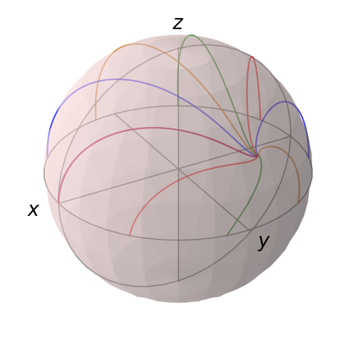
(a) purely collective

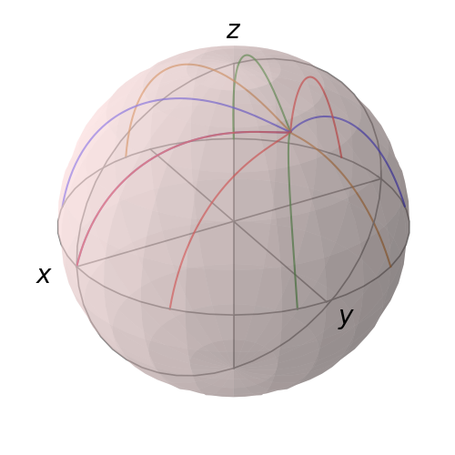
(b) local decay $\gamma_{+}=0.2B$

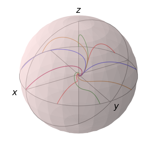
(c) local dephasing $\gamma_{z}=0.4B$

Figure 1: Solutions of the mean-field equations (22) depicted on the unit ball. As collective parameters we choose $\vec{B}=B/\sqrt{2}(\vec{e}_{z}-\vec{e_{x}})$, $\kappa_{+}=0.8B$ and $\kappa_{-}=0$. (a) Only collective processes are present $\gamma_{i}=0$ so that the trajectories stay on the surface of the ball. (b) Due to the local decay, the stable fixed point lies inside the ball. (c) If local dephasing is present, all trajectories approach the fully mixed state $r=0$.

V Exact semi-classical regime

(a) $B_{x}=-0.8\kappa_{+}$

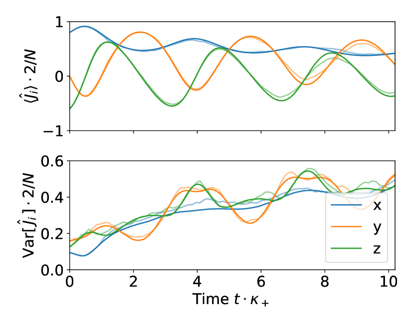
(b) $B_{x}=-2.4\kappa_{+}$

Figure 2: Numerical solution of the master equation (1) with the classical stochastic trajectories obeying Eq. (27). The light and bold curves are averaged over 100 and 10000 sampled trajectories, respectively. The initial state is a spin coherent state. In both figures we choose the parameters $N=40$, $\kappa_{z}=\kappa_{+}$ and $B_{y}=B_{z}=0$. There are no non-collective processes $\gamma_{\pm,z}=0$.

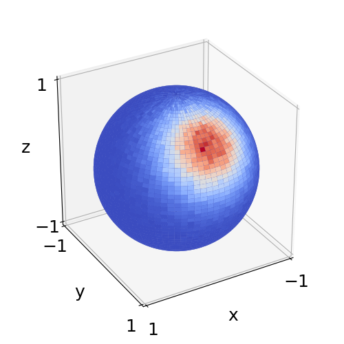
(a) $N=20$

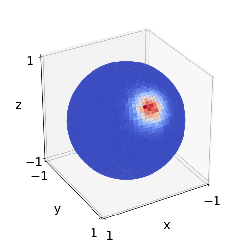
(b) $N=100$

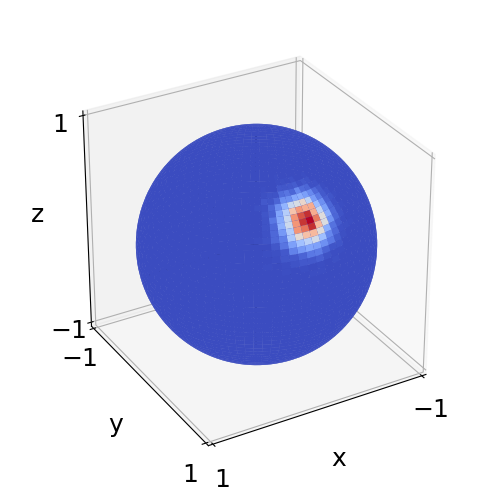
(c) $N=200$

Figure 3: The pictures show the P-function of the steady state as a function on the sphere ($|\vec{r}|=1$) for three different system sizes $N$. All other parameters are the same as in Fig. 2 (a). The width of the distribution is decreasing when $N$ is increasing.

Going beyond mean-field one must include the diffusion term in the $P$-function evolution equation. This term is generated by collective dissipation in the master equation (1). Using spherical coordinates, the diffusion matrix reads

$$\left(\begin{array}[]{ccc}\frac{2\left(1-\eta^{2}\right)(\eta(\kappa_{-}-\kappa_{+})+r(\kappa_{-}+\kappa_{+}))}{r}&0&-\left(\eta^{2}-1\right)\left(r^{2}-1\right)(\kappa_{-}-\kappa_{+})\\ 0&2\kappa_{z}+2\frac{\eta(\kappa_{-}(\eta r+1)+\kappa_{+}(\eta r-1))}{\left(1-\eta^{2}\right)r}&0\\ -\left(\eta^{2}-1\right)\left(r^{2}-1\right)(\kappa_{-}-\kappa_{+})&0&0\\ \end{array}\right)\,.$$ (23)

If the diffusion matrix is not positive semidefinite, the partial differential equation is no longer parabolic and numerical solution with, for example, finite element methods, is unstable. There exist parameter regimes where this matrix has only positive eigenvalues. In this case the dynamics is described by a Fokker-Planck equation and can be solved with stochastic methods. An obvious example is the case of dephasing only, i.e. $\kappa_{-}=\kappa_{+}=0$. Dephasing can be realized by a stochastic unitary evolution Strunz (2005); Grotz et al. (2006); Müller et al. (2019). The corresponding stochastic Hamiltonian is non-interacting, so that the full dynamics can be mapped to a classical stochastic process. This is reflected by the positivity of the diffusion matrix. More generally, whenever the loss and the pump rates are identical $\kappa_{+}=\kappa_{-}$, the diffusion is positive.
Let us now focus on the purely collective case with no local decay processes. Then the Fokker-Planck equation preserves the radial direction $r$, so that we can set $r=1$ and recover the canonical spin coherent state $P$-function. Then, the matrix (23) has two non-zero eigenvalues given by

$$\lambda_{1} =2(1-\eta^{2})((1+\eta)\kappa_{-}+(1-\eta)\kappa_{+})\,,$$ (24)

$$\lambda_{2} =2\kappa_{z}+\kappa_{-}\frac{2\eta}{1-\eta}-\kappa_{+}\frac{2\eta}{1+\eta}\,.$$ (25)

We see that Eq. (19) is a proper Fokker-Planck equation if both $\lambda_{1},\lambda_{2}$ are positive. $\lambda_{1}$ is always positive since $-1\leq\eta\leq 1$ and $\lambda_{2}$ is positive for all $\eta$ and $\phi$ if

$$\kappa_{+}+\kappa_{-}\leq 2\kappa_{z}\,.$$ (26)

Satisfying this condition, the open quantum system evolution described by Eq. (1) can be mapped to a classical diffusion process on the sphere. Nevertheless the state lies in a finite-dimensional Hilbert-space and contains quantum fluctuations due to the non-zero overlap of coherent states. Relation (26) can be understood in the sense that one simply has to add enough dephasing to compensate the positivity violation of the diffusion matrix due to collective losses. We point out that adding dephasing does however not influence the mean-field theory and thus the different phases of the model.
The standard way of solving the Fokker-Planck equation is to consider the set of stochastic differential equations

$${\rm d}\eta =a_{\eta}{\rm d}t+\sqrt{\frac{\lambda_{1}}{N}}{\rm d}\xi_{\eta}\,,$$ (27)

$${\rm d}\phi =a_{\phi}{\rm d}t+\sqrt{\frac{\lambda_{2}}{N}}{\rm d}\xi_{\phi}\,,$$ (28)

where ${\rm d}\xi_{i}$ is a real Ito increment with properties ${\rm d}\xi_{i}{\rm d}\xi_{j}=\delta_{ij}{\rm d}t$ and the drift terms are given in appendix B. In the absence of the noise terms we obtain again the mean-field theory, as in the last section. The stochastic equations provide an efficient way of calculating the $P$-function of the system for any system size $N$ when condition (26) is satisfied. Since in Eq. (27) $N$ is merely a parameter determining the strength of the diffusion, the numerical effort for computing the state with this stochastic method is independent of the dimension of the underlying Hilbert-space. The method becomes more efficient than direct numerical integration of the master equation for moderate system sizes, i.e. when the mean field approximation is not yet applicable. We find that expectation values converge quickly with respect to the number of sampled trajectories, as we can see from the following example.
We consider the cooperative resonance fluorescence model Walls et al. (1978); Walls (1980); Drummond and Carmichael (1978); Carmichael (1980) with additional collective dephasing. The model is described by the master equation (1) with $\kappa_{-}=B_{y}=B_{z}=0$, $\kappa_{+}=\kappa_{z}$ and without non-collective terms $\gamma_{+}=\gamma_{-}=\gamma_{z}=0$. It features a mirror symmetry $J_{x}\rightarrow-J_{x}$ which is spontaneously broken when the driving exceeds the collective damping $|B_{x}|>\kappa_{+}$. If the damping is large, as in Fig. 2 (a), a localized steady state is reached as predicted by mean-field theory. In the symmetry broken regime the dynamics is characterized by damped oscillations towards a steady state with large variance, as seen in Fig. 2 (b). This is an example where the mean field theory does not predict correctly the steady state and the finite system size remains relevant even for large $N$, see Ref. Link et al. (2019) for a more detailed discussion.
In Fig. (3) we show an example of a steady state P-function of the model as a density on the sphere for different system sizes, in the case of large damping ($|B_{x}|>\kappa_{+}$). As the system size $N$ increases, the distribution gets more localized due to weaker diffusion. For large system sizes the steady state distribution is sharply peaked at the stable fixed point of the corresponding mean-field theory.

VI Discussion

In this article we have further developed a particular phase space picture for driven dissipative spin systems first introduced in the context of laser theory Haken et al. (1967). Our approach incorporates both collective and permutation invariant local decay processes into a unified framework, which allows for a very simple derivation of evolution equations for the corresponding $P$-function.
As is well known, the coefficient matrix for the second order terms in the equation of motion for phase space quasiprobability distributions is typically not positive semidefinite. We have examined conditions under which initially positive phase space densities remain positive for all times. Then the dynamics can be considered classical in the sense that no entanglement is generated between the two-level systems. In particular, in the case of purely collective dynamics, presence of sufficiently large dephasing ensures the positivity. Another interesting case is the ’infinite temperature’ limit $\kappa_{+}=\kappa_{-}$, which results in positive diffusion even in presence of non-collective processes. In case the diffusion matrix is not positive, solving the problem using phase space techniques is challenging as this leads to regions where $P$ is negative and the evolution equation is no longer parabolic.
The phase space approach provides immediately a consistent mean field picture just by neglecting the subleading second order terms in the evolution equation. By analyzing the stability of the fixed points of the mean field equations, phase diagrams for non-equilibrium phases can be obtained. However, scenarios are known where finite-size corrections become relevant even for large system sizes Link et al. (2019). In the case of positive diffusion, such finite-size corrections can be incorporated exactly by adding noise to the mean-field equation. This remarkable feature allows to efficiently solve the problem with stochastic methods, where the numerical effort is independent of the dimension of the underlying Hilbert space.
The formalism presented in this paper can be straightforwardly generalized for $\text{SU}(n)$-type models Barry and Drummond (2008); Grass et al. (2013), by using generalized Bloch-representations, for example for three-level systems, and defining the coherent states accordingly.
We believe that the presentation of the phase space methods in this article is easily accessible and can be applied effortlessly to problems of current experimental and theoretical interest.

Appendix A Drift and diffusion in xyz parameterization

In this appendix we provide the full expressions for the diffusion matrix and the drift term. These can be derived by expressing the action of the generator of master equation (1) onto a spin coherent state

$$\mathcal{L}\alpha(\vec{r})=\Big{(}\partial_{i}a_{i}(\vec{r})+\frac{1}{2N}\partial_{i}\partial_{j}D_{ij}(\vec{r})\Big{)}\alpha(\vec{r})\,.$$ (29)

Expressing the state via (13), this results in an evolution equation for the $P$-function of model (1)

$$\partial_{t}P(\vec{r})=\Big{(}-\partial_{i}a_{i}(\vec{r})+\frac{1}{2N}\partial_{i}\partial_{j}D_{ij}(\vec{r})\Big{)}P(\vec{r})\,.$$ (30)

The drift term $\vec{a}$ reads

$$\begin{split}&a_{x}={B_{y}}z-{B_{z}}y+\frac{x(-\kappa_{+}-\kappa_{z}+(N-1)z(\kappa_{-}-\kappa_{+}))-\kappa_{-}x}{N}+x(\gamma_{-}-\gamma_{+}-\gamma_{z})\,,\\ &a_{y}=-{B_{x}}z+{B_{z}}x+\frac{+y(-\kappa_{+}-\kappa_{z}+(N-1)z(\kappa_{-}-\kappa_{+}))-\kappa_{-}y}{N}+y(\gamma_{-}-\gamma_{+}-\gamma_{z})\,,\\ &a_{z}={B_{x}}y-{B_{y}}x+\frac{-2\kappa_{-}+2\kappa_{+}+\kappa_{-}\left(-(N-1)\left(x^{2}+y^{2}\right)-2z\right)+\kappa_{+}\left((N-1)\left(x^{2}+y^{2}\right)-2z\right)}{N}\\ &\qquad+2\gamma_{-}(z-1)-2\gamma_{+}(z+1)\,,\\ \end{split}$$ (31)

and the symmetric diffusion matrix $D=D^{T}$ is given as

$$\begin{split}&D_{xx}=2\left(\kappa_{-}z\left(-x^{2}+z+1\right)+\kappa_{+}z\left(x^{2}+z-1\right)+\kappa_{z}y^{2}\right)\,,\\ &D_{xy}=-2xy(\kappa_{z}+z(\kappa_{-}-\kappa_{+}))\,,\\ &D_{xz}=x\left(\kappa_{-}\left(x^{2}+y^{2}-(z+1)^{2}\right)-\kappa_{+}\left(x^{2}+y^{2}-(z-1)^{2}\right)\right)\,,\\ &D_{yy}=2\left(\kappa_{z}x^{2}+\kappa_{-}z\left(-y^{2}+z+1\right)+\kappa_{+}z\left(y^{2}+z-1\right)\right)\,,\\ &D_{yz}=y\left(\kappa_{-}\left(x^{2}+y^{2}-(z+1)^{2}\right)-\kappa_{+}\left(x^{2}+y^{2}-(z-1)^{2}\right)\right)\,.\\ &D_{zz}=2\left(x^{2}+y^{2}\right)(\kappa_{-}+\kappa_{+}+\kappa_{-}z-\kappa_{+}z)\,.\end{split}$$ (32)

Appendix B Drift and diffusion in spherical parameterization

Parameterizing the spin coherent state with spherical coordinates as in (12), we can transform the derivatives in (29) accordingly. Expressing the state as

$$\rho=\int{\rm d}\eta\int{\rm d}\phi\int{\rm d}r\,\alpha(\vec{r})P(\eta,\phi,r)\,,$$ (33)

the $P$-function obeys an evolution equation of the same form as (19). In particular

$$\partial_{t}P=\Big{(}-\sum_{\beta={\eta,\phi,r}}\partial_{\beta}a_{\beta}+\sum_{\beta,\beta^{\prime}={\eta,\phi,r}}\frac{1}{2N}\partial_{\beta}\partial_{\beta^{\prime}}D_{\beta,\beta^{\prime}}\Big{)}P\,,$$ (34)

with drift

$$\begin{split}&a_{\eta}=\sqrt{1-\eta^{2}}({B_{y}}\cos(\phi)-{B_{x}}\sin(\phi))+2\gamma_{-}(\eta r-1)-2\gamma_{+}(\eta r+1)-\frac{1}{2}\left(\eta^{2}-1\right)r(\kappa_{-}-\kappa_{+})\\ &\qquad+\frac{2(\kappa_{-}-\kappa_{+})+2\eta(\eta(\kappa_{-}-\kappa_{+})+2r(\kappa_{-}+\kappa_{+}))}{2Nr}\,,\\ &a_{\phi}=\frac{-\sqrt{1-\eta^{2}}\eta({B_{x}}\cos(\phi)+{B_{y}}\sin(\phi))-{B_{z}}\eta^{2}+{B_{z}}}{\eta^{2}-1}\,,\\ &a_{r}=-2\eta(\gamma_{-}+\gamma_{+})+\left(\eta^{2}+1\right)r(\gamma_{-}-\gamma_{+})+\gamma_{z}\left(\eta^{2}-1\right)r\,,\\ \end{split}$$ (35)

and diffusion (c.f. Eq. (23))

$$\begin{split}&D_{\eta,\eta}=-\frac{2\left(\eta^{2}-1\right)(\eta(\kappa_{-}-\kappa_{+})+r(\kappa_{-}+\kappa_{+}))}{r}\,,\\ &D_{\phi,\phi}=-\frac{2\left(\eta(\kappa_{-}-\kappa_{+})+\eta^{2}r(\kappa_{-}+\kappa_{+}-\kappa_{z})+\kappa_{z}r\right)}{\left(\eta^{2}-1\right)r}\,,\\ &D_{\eta,r}=\left(\eta^{2}-1\right)\left(-\left(r^{2}-1\right)\right)(\kappa_{-}-\kappa_{+})\,,\\ &D_{\phi,\eta}=D_{\phi,r}=D_{r,r}=0\,.\end{split}$$ (36)

References

- Dicke (1954) R. H. Dicke, Phys. Rev. 93, 99 (1954).
- Dimer et al. (2007) F. Dimer, B. Estienne, A. S. Parkins, and H. J. Carmichael, Phys. Rev. A 75, 013804 (2007).
- Baumann et al. (2010) K. Baumann, C. Guerlin, F. Brennecke, and T. Esslinger, Nature 464, 1301 (2010).
- Nataf et al. (2019) P. Nataf, T. Champel, G. Blatter, and D. M. Basko, Phys. Rev. Lett. 123, 207402 (2019).
- Johnson et al. (2019) A. Johnson, M. Blaha, A. E. Ulanov, A. Rauschenbeutel, P. Schneeweiss, and J. Volz, Phys. Rev. Lett. 123, 243602 (2019).
- Lalumière et al. (2013) K. Lalumière, B. C. Sanders, A. F. van Loo, A. Fedorov, A. Wallraff, and A. Blais, Phys. Rev. A 88, 043806 (2013).
- Galve et al. (2017) F. Galve, A. Mandarino, M. G. A. Paris, C. Benedetti, and R. Zambrini, Scientific Reports 7, 42050 (2017).
- Shammah et al. (2018) N. Shammah, S. Ahmed, N. Lambert, S. De Liberato, and F. Nori, Phys. Rev. A 98, 063815 (2018).
- Mandel and Wolf (1995) L. Mandel and E. Wolf, Optical Coherence and Quantum Optics (Cambridge University Press, 1995).
- Meiser and Holland (2010) D. Meiser and M. J. Holland, Phys. Rev. A 81, 033847 (2010).
- Iemini et al. (2018) F. Iemini, A. Russomanno, J. Keeling, M. Schirò, M. Dalmonte, and R. Fazio, Phys. Rev. Lett. 121, 035301 (2018).
- Link et al. (2019) V. Link, K. Luoma, and W. T. Strunz, Phys. Rev. A 99, 062120 (2019).
- Tucker et al. (2018) K. Tucker, B. Zhu, R. J. Lewis-Swan, J. Marino, F. Jimenez, J. G. Restrepo, and A. M. Rey, New Journal of Physics 20, 123003 (2018).
- Gorini et al. (1976) V. Gorini, A. Kossakowski, and E. C. G. Sudarshan, Journal of Mathematical Physics 17, 821 (1976).
- Lindblad (1976) G. Lindblad, Commun. Math. Phys. 48, 119 (1976).
- Gisin and Cibils (1992) N. Gisin and M. B. Cibils, Journal of Physics A: Mathematical and General 25, 5165 (1992).
- Puri and Lawande (1980) R. R. Puri and S. V. Lawande, Physica A 101, 599 (1980).
- Walls et al. (1978) D. F. Walls, P. D. Drummond, S. S. Hassan, and H. J. Carmichael, Progress of Theoretical Physics Supplement 64, 307 (1978).
- Walls (1980) D. F. Walls, Journal of Physics B: Atomic and Molecular Physics 13, 2001 (1980).
- Drummond and Carmichael (1978) P. Drummond and H. Carmichael, Optics Communications 27, 160 (1978).
- Carmichael (1980) H. J. Carmichael, Journal of Physics B: Atomic and Molecular Physics 13, 3551 (1980).
- Weidlich et al. (1967a) W. Weidlich, H. Risken, and H. Haken, Z. Angew. Phys. 201, 396 (1967a).
- Weidlich et al. (1967b) W. Weidlich, H. Risken, and H. Haken, Z. Phys. A: Hadrons Nucl. 204, 223 (1967b).
- Haken et al. (1967) H. Haken, H. Risken, and W. Weidlich, Z. Angew. Phys. 206, 355 (1967).
- Patra et al. (2019) A. Patra, B. L. Altshuler, and E. A. Yuzbashyan, Phys. Rev. A 99, 033802 (2019).
- Zhang et al. (1990) W.-M. Zhang, D. H. Feng, and R. Gilmore, Rev. Mod. Phys. 62, 867 (1990).
- Hannukainen and Larson (2018) J. Hannukainen and J. Larson, Phys. Rev. A 98, 042113 (2018).
- Ferreira and Ribeiro (2019) J. S. Ferreira and P. Ribeiro, Phys. Rev. B 100, 184422 (2019).
- Strunz (2005) W. T. Strunz, Open Systems & Information Dynamics 12, 65 (2005), https://doi.org/10.1007/s11080-005-0487-1 .
- Grotz et al. (2006) T. Grotz, L. Heaney, and W. T. Strunz, Phys. Rev. A 74, 022102 (2006).
- Müller et al. (2019) K. Müller, K. Luoma, and W. T. Strunz, “Geometric phase gates in dissipative quantum dynamics,” (2019), arXiv:1907.08033 [quant-ph] .
- Barry and Drummond (2008) D. W. Barry and P. D. Drummond, Phys. Rev. A 78, 052108 (2008).
- Grass et al. (2013) T. Grass, B. Juliá-Díaz, M. Ku, and M. Lewenstein, Phys. Rev. Lett. 111, 090404 (2013).