Spectral shapes of the Lyman-alpha emission from galaxies: I. blueshifted emission and intrinsic invariance with redshift

Abstract

We demonstrate the redshift-evolution of the spectral profile of H i Lyman-alpha (Ly$\alpha$) emission from star-forming galaxies. In this first study we pay special attention to the contribution of blueshifted emission. At redshift $z=2.9-6.6$, we compile spectra of a sample of 229 Ly$\alpha$-selected galaxies identified with the Multi-Unit Spectroscopic Explorer at the Very Large Telescope, while at low-$z$ ($<0.44$) we use a sample of 74 ultraviolet-selected galaxies observed with the Cosmic Origin Spectrograph onboard the Hubble Space Telescope. At low-$z$, where absorption from the intergalactic medium (IGM) is negligible, we show that the ratio of Ly$\alpha$ luminosity bluewards and redwards of line center ($L_{\mathrm{B/R}}$) increases rapidly with increasing equivalent width ($W_{\mathrm{Ly}\alpha}$). This correlation does not, however, emerge at $z=3-4$, and we use bootstrap simulations to demonstrate that trends in $L_{\mathrm{B/R}}$ should be suppressed by variations in IGM absorption. Our main result is that the observed blueshifted contribution evolves rapidly downwards with increasing redshift: $L_{\mathrm{B/R}}$ $\approx 30$ % at $z\approx 0$, but drops to 15 % at $z\approx 3$, and to below 3 % by $z\approx 6$. Applying further simulations of the IGM absorption to the unabsorbed COS spectrum, we demonstrate that this decrease in the blue-wing contribution can be entirely attributed to the thickening of intervening Ly$\alpha$ absorbing systems, with no need for additional H i opacity from local structure, companion galaxies, or cosmic infall. We discuss our results in light of the numerical radiative transfer simulations, the evolving total Ly$\alpha$ and ionizing output of galaxies, and the utility of resolved Ly$\alpha$ spectra in the reionization epoch.

1 Introduction

The Ly$\alpha$ emission line, and its spectral profile, encode a wealth of information about both star-formation and various gas phases in galaxies, including the interstellar medium (ISM), the more tenuous circumgalactic medium (CGM) and, at the highest redshifts, the intergalactic medium (IGM). Because of the abundance of atomic hydrogen and the nature of the H i atom, Ly$\alpha$ is intrinsically the brightest spectral feature of ionized nebulae, but also has the largest optical depth to absorption. Ly$\alpha$ is therefore sufficiently luminous to be observed from redshifts ($z$) out to above 9 (e.g. Hashimoto et al., 2018), but is then multiply scattered by H i atoms, and re-shaped by radiative transfer (RT) effects into which many galaxy properties enter (see Runnholm et al. 2020b for a thorough investigation, and Dijkstra 2014 and Hayes 2015 for reviews).

This absorption by H i may occur in both ‘conventional’ (=H i-dominated) atomic gas clouds or residual H i ions in H ii-dominated gas. The Ly$\alpha$ RT, therefore, can be a problem covering various regions and physical scales. The emergent Ly$\alpha$ line profile will firstly be a reflection of the kinematics of the H ii regions in which Ly$\alpha$ is intrinsically produced. However this velocity profile is subsequently modulated by scattering events within the H ii region itself, that will introduce some degree of broadening depending upon the small scale gas densities. But Ly$\alpha$ photons may also have to traverse high column density, optically thick gas, that permits escape only after long excursions in frequency space (wing scatterings Adams, 1972; Neufeld, 1990). This generally high optical depth at line center introduces double-peaked profiles, consisting of blueshifted and redshifted components with little emission at line center ($\Delta v=0$), and a separation that depends on the H i column density ($N_{\mathrm{HI}}$). Because gas is rarely static or homogeneous in the ISM, the density distribution, clumpiness, and dynamics of the neutral and dense ionized medium in galaxies will all influence the line profile. As starburst galaxies typically show moderate-velocity outflowing media (see reviews by Rupke 2018 and Veilleux et al. 2020 at low-$z$; Erb 2015 at high-$z$) stronger redshifted Ly$\alpha$ peaks, with secondary weaker blue components, are commonplace.

Because the blueshifted component of Ly$\alpha$ is easily suppressed by scattering in outflowing material, significant emission bluewards of the Ly$\alpha$ line center ($\Delta v<0$) is relatively rare, and has become a key signpost of a low gas column density. Henry et al. (2015) first obtained UV spectra of a sample of ‘Green Pea’ galaxies: not only do these galaxies exhibit among the strongest Ly$\alpha$ lines known (average Ly$\alpha$ escape fraction of $\approx 25$% and EW of $\approx 60$ Å), but a remarkable fraction of 9/10 also show double peaks. Similar results have since been presented in other low-$z$ samples with similarly strong nebular EWs, and also high [O iii]/[O ii] ratios (Yang et al., 2017b; Jaskot et al., 2017; Izotov et al., 2018, 2020). In Lyman break galaxies (LBG) at $z=2-3$, the relative contribution of blueshifted Ly$\alpha$ (defined as the ratio of equivalent widths at velocities bluewards and redwards of line center) also correlates strongly with the Ly$\alpha$ EW (Erb et al., 2014), and becomes even more prominent in very highly ionized galaxies (Erb et al., 2016; Trainor et al., 2016). These associations are also borne out by theoretical calculations and models. Verhamme et al. (2015) used Ly$\alpha$ radiation transfer simulations to show that a narrow velocity separation between two spectrally resolved peaks could be used as a signifier of column densities close to the limit of optical thickness at the Lyman edge; see Osterbrock (1962) and Hummer & Rybicki (1971) for the original discussions in the low optical depth limits. The implication that galaxies with narrow Ly$\alpha$ separations of below $\approx 250$ km s^-1  would be Lyman continuum (LyC) emitting galaxies was qualitatively borne out by recent observations (e.g. Izotov et al. 2018, see also Jaskot et al. 2019) and further theoretical work (e.g. Kimm et al., 2019; Kakiichi & Gronke, 2019). As optical emission lines are hard to detect with high fidelity at $z\gtrsim 6$ because of redshifting to the IR, and absorption lines being equally hard because of the faint continuum, the Ly$\alpha$ spectral profile is a promising diagnostic for LyC emission at high-$z$.

Because Ly$\alpha$ is absorbed by H i, and the ionized fraction of the universe evolves with redshift, Ly$\alpha$ is a natural probe of the epoch of reionization (EoR; most recently reviewed by Dijkstra 2014). Studies began using first-order tests of the evolving Ly$\alpha$ luminosity function (LF; e.g. Kashikawa et al. 2006; Malhotra & Rhoads 2004, 2006) but, in light of the fact that galaxies may also assemble rapidly near the EoR, moved on to differential tests of Ly$\alpha$ evolution with respect to the underlying galaxy population. This has been cast as either the ‘volumetric’ Ly$\alpha$ escape fraction (Hayes et al., 2011; Dijkstra & Jeeson-Daniel, 2013; Konno et al., 2016; Wold et al., 2017) or as the fraction of strong LAEs among LBGs (Stark et al., 2010; Ono et al., 2012; Curtis-Lake et al., 2012; Schenker et al., 2012; Pentericci et al., 2014; De Barros et al., 2017; Mason et al., 2018; Kusakabe et al., 2020).

While the evolution of the average Ly$\alpha$ output may probe the neutral gas content of the universe at a certain redshift, reionization was also inherently patchy because of the clustering of both cosmic gas and ionizing sources. Thus we need to ultimately progress beyond single averages at a given cosmic time (as in the studies above). Given that the EoR history and topology is a function of both structural over-density (including gas) and galaxy formation, it naturally follows that the blunt measure of neutral fraction vs time will vary with position (analogous to downsizing). Ultimately it must give way to a more nuanced approach, accounting for spatial/environmental, as well as temporal, variation. Ly$\alpha$ spectroscopy most likely offers the solution here, but in the form of a more detailed, spectrally resolved approach that targets the line profile.

To kick-start this science, a number of double-peaked Ly$\alpha$ emission lines have recently been identified at high-$z$. These include Aerith B at $z=5.8$ (Bosman et al., 2020), NEPLA4 at $z=6.5$ (Songaila et al., 2018) and COLA1 at $z=6.6$ (Hu et al., 2016), which all show impressive Ly$\alpha$ double-peaks, strongly resemblant of the $z\approx 0$ compact starbursts (Henry et al., 2015; Jaskot et al., 2017; Izotov et al., 2020). According to simplified, homogeneous prescriptions for the neutral fraction of the universe at these redshifts, these profiles should not exist, and even in modern radiation hydrodynamic simulations of the EoR, blue peaks at $z\gtrsim 6$ are rare (Gronke et al., 2020). Clearly the reionization progression is patchy, and Aerith B is a perfect example, being discovered inside the proximity zone of a luminous quasar. Bagley et al. (2017) recently calculated the bubble sizes necessary to explain the existence of two very luminous Ly$\alpha$-emitter at $z\approx 6.4$, finding they must exist on Mpc scales. Matthee et al. (2018) performed a similar study using the spectral profile of COLA1 including its blue Ly$\alpha$ bump, and found comparable if somewhat smaller values; their calculation was revised upwards very recently by Mason & Gronke (2020) whose Bayesian inference places additional new constraints on the ionizing output and neutral fraction within the H ii bubble, as well as the bubble radius itself.

The uncertainties and degeneracies in these approaches are significant, but will doubtless improve as more systems are discovered and data improve. While the universe beyond $z\approx 5$ is really the point of interest, these studies can be significantly informed by those from low- and mid-$z$. Specifically with regard to the Ly$\alpha$ profile analysis, it is never clear at high-$z$ how much absorption can be attributed to the IGM, and how much is simply frequency redistribution in the ISM/CGM. Because galaxy populations evolve in many ways – mass, morphology, dust content, etc – we do not believe a priori that Ly$\alpha$ profiles from low-$z$ should necessarily hold in a galaxy population that is 10 times younger/less evolved. However, it remains well-motivated to see how the high-$z$ observables would look in the no-evolution case. We do not currently have the data to probe these effects deep into the EoR, but are able to test the evolution of the Ly$\alpha$ spectral profile out to $z\gtrsim 6$ with existing large samples, which is very much the first step.

In this paper we study the evolution of the Ly$\alpha$ spectral line shape with redshift, and the impact of absorption from discrete H i-absorbing systems in the IGM. We use large samples of homogeneously-selected Ly$\alpha$ spectra that have recently become available: at high-$z$ we adopt the MUSE-WIDE data (Urrutia et al. 2019; see also Herenz et al. 2017) in the CANDELS-Deep region of the GOODS-South field. These data provide spectra with resolving powers of $R(\equiv\lambda/\Delta\lambda)=1800$-3500 over 44 arcmin², of 478 galaxies. For a baseline Ly$\alpha$ spectrum that is not attenuated by the IGM, we leverage various samples of low-$z$ spectra observed with HST/COS. These observations are pointed at pre-selected galaxies, but have higher spectral resolving power ($R$ up to 22,000) and are also obtained at redshifts where the IGM has little or no impact on the Ly$\alpha$ spectral profile.

We present an overview of the data and samples in Section 2, and describe the measurements we make and methods we use in Section 3, which mainly relate to estimating systemic redshifts and simulating the IGM. In Section 4 we present an overview of the basic Ly$\alpha$ properties of the high- and low-$z$ samples. We describe the shapes of the ensemble Ly$\alpha$ profiles as a function of other key Ly$\alpha$ observables in Section 5. We present our results concerning redshift evolution in Section 6, where we mainly show that low-$z$ spectral profiles, and a simply simulated IGM, can entirely reproduce the evolution of the Ly$\alpha$ spectral shape out to $z=6$. In Section 7 we discuss these results in light of existing Ly$\alpha$ radiation transfer simulations and current knowledge of the IGM opacity. Section 8 presents some thoughts on the future application and limitations of our approach, and we present a final summary of our findings in Section 9. We adopt cosmological parameters of $\{H_{0},~{}\Omega_{\mathrm{M}},~{}\Omega_{\Lambda}\}=\{70~{}\mathrm{km~{}s^{-1}~{}Mpc^{-1}},~{}0.3,~{}0.7\}$.

2 Observational Data

For this paper we draw upon a large compilation of data. We use HST/COS for low-$z$ spectroscopy of the Ly$\alpha$ line, and VLT/MUSE for Ly$\alpha$ spectroscopy at high-$z$. As the UV continuum of the high-$z$ sample is relatively faint, we use deep imaging from HST/ACS to determine the UV magnitudes of the Ly$\alpha$-emitting galaxies at $z>2.9$. We now describe the origin, assembly, and processing of these data in turn.

2.1 The low-z reference data: HST/COS

2.1.1 Sample Overview

HST/COS (Green et al., 2012) is an ultraviolet spectrograph onboard HST and in the settings we use provides spectra of moderate nominal resolution, with $R\approx$ 18,000 on average, for point-sources. It has a 2$\farcs$5 diameter entrance aperture, which naturally will sample a range of spatial scales, depending upon the redshift of the galaxy, which varies from object to object. Galaxies observed with HST/COS have all been pre-selected by the HST observers and identified as the best targets with a certain scientific objective in mind.

The COS data are drawn from the following general observer programs (with principal investigators in parentheses): GO 11522 (PI: Green), 11727 (Heckman), 12027 (Green), 12269 (Scarlata), 12583 (Hayes), 12928 (Henry), 13017 (Heckman), 13293 (Jaskot), 13744 (Thuan), 14080 (Jaskot), 14201 (Malhotra), 14635 (Izotov), 15136 (Izotov). Most of the spectra have been published in studies of galaxy winds and outflows, as well as their relation to Ly$\alpha$ output and kinematic properties (Heckman et al., 2011, 2015; Wofford et al., 2013; Rivera-Thorsen et al., 2015, 2017; Henry et al., 2015; Jaskot & Oey, 2014; Jaskot et al., 2017, 2019; Izotov et al., 2016, 2018; Yang et al., 2017b, and more). It is beyond the scope of this paper to summarize the results of these studies but the selection identifies galaxies in the redshift range between $z=0.020$ and $z=0.44$, with a median value of $z=0.177$. This places the Ly$\alpha$ emission line in either the G130M or G160M grating of COS, and delivers a spectral resolution for point-sources between $R=$13,000 and 22,000 depending upon lifetime position and redshift. This resolution, however, depends on spatial extent of the source compared to the aperture, which for Ly$\alpha$ is uncertain and the actual resolution is unknown in practice. We discard low-resolution spectra obtained with the G140L grating, which has also been obtained in some of the programs for a handful galaxies.

The large majority of the targets were selected by UV emission, usually from GALEX far-UV photometry but also slit-less spectroscopy of Ly$\alpha$ in the case of GO 12269. Most were also constrained in at least redshift by optical line emission, which almost exclusively comes from the Sloan Digital Sky Survey (SDSS). Further constraints may have been applied in terms of optical compactness, H$\alpha$ or [O iii] equivalent widths, [O iii]/[O ii] ratios, and more. Attending mainly to the papers above, star formation rates (SFR) lie in the range from 0.1 to over 50 M_⊙ yr^-1.

2.1.2 Reduction and basic processing

All spectra were obtained from the Mikulski Archive for Space Telescopes (MAST), and reduced homogeneously with the calibration pipeline (CALCOS), v.3.3.7. Systemic redshifts have been derived from simultaneously fitting up to 20 optical emission lines for sources with SDSS spectra, and from literature values (e.g. Cowie et al., 2011), otherwise. More details can be found in Runnholm et al. (2020a).

We first correct the COS spectra for Milky Way foreground extinction, by looking up the mean $E_{B-V}$ at the target coordinates from the maps of Schlafly & Finkbeiner (2011, using the irsa_dust interface in astroquery) and applying the Cardelli et al. (1989) extinction law. No correction for internal extinction is made. We continuum-subtract the COS spectra by fitting low-order polynomial functions to the continuum over the wavelength range of $\lambda>1219$ Å, and avoiding strong stellar and interstellar features. The COS sample was mostly UV-selected as discussed above, and the galaxies are not guaranteed to have Ly$\alpha$ in emission; as Ly$\alpha$ emission is mandatory for this study we discard all galaxies with signal-to-noise ratio in Ly$\alpha$ less than 8. This leaves a sub-sample of 74 galaxies, for which the median Ly$\alpha$ luminosity is $1.25\times 10^{42}$ erg s^-1.

2.2 High-z Ly$\alpha$ information from MUSE

2.2.1 Sample Overview

Unlike HST/COS, VLT/MUSE (Bacon et al., 2010, 2014) is a survey instrument. It is the first truly large-format integral field spectrograph, with a field-of-view of $60\times 60$ arcsec². MUSE therefore delivers an emission line survey for Ly$\alpha$-emitting galaxies between $z=2.9$ and $z=6.6$ with 100 % spectroscopic completeness. However the spectral resolution is somewhat lower than that of COS, and varies between $R=1800$ at the blue end, and 3500 at the red end.

Many Ly$\alpha$ surveys have already been conducted with MUSE, but here we rely upon the MUSE-WIDE survey (Herenz et al., 2017; Urrutia et al., 2019). The main reasons is that there are many pointings (44 fields), that are observed to a homogeneous depth (1-hour per pointing). The 1-dimensional data are easily accessible through the CDS/VisieR database.

2.2.2 Basic processing

MUSE-WIDE LAEs are continuum-subtracted using the same polynomial-fitting method as the COS spectra (Section 2.1). The Ly$\alpha$ luminosity is measured by numerical integration over a window that is 2500 km s^-1 wide, and the errors are estimated by end-to-end Monte Carlo simulations. As with the COS spectra, we retain only spectra for which the SNR in Ly$\alpha$ exceeds 8. This leaves a sub-sample of 229 galaxies, for which the median Ly$\alpha$ luminosity is $3.1\times 10^{42}$ erg s^-1.

We examined the MUSE-WIDE webpages to determine the sky conditions and data quality when the data were obtained. Using the SQL query interface we determine that 42 of the 44 fields were observed under either photometric or clear conditions, implying the large majority of the LAEs in our sample should have good photometric accuracy. The MUSE-WIDE team has contrasted synthetic photometry of the Data Release 1 spectra with HST magnitudes of brighter stars, finding generally good agreement: the final dispersion in flux is on the order of 5 %, with all but a handful of sources agreeing to better than 10 % (T. Urrutia & L. Wisotzki, private communication). We also note that the main results of this paper are based upon normalized spectra, for which absolute photometric accuracy is not vital.

We finally note that this Ly$\alpha$ selection at high-$z$, and UV selection at low-$z$, are very different strategies for identifying galaxies. This may introduce some bias, but is a necessary condition of contrasting low-$z$ samples with large datasets at high-$z$ with current facilities. We later perform an additional level of matching between the two samples; see Section 5.3 for more details.

2.3 High-z continuum information from HST/ACS

Because the high-$z$ targets are selected based upon flux in the Ly$\alpha$ line, a subset of the sample will be faint or undetected in the continuum when examining the same spectroscopic data. The consequence is that the EWs measured from the spectra themselves (see Section 3.1) will become more imprecise towards faint magnitudes, and instead we adopt the UV luminosities from HST broadband imaging. The objects in the Urrutia et al. (2019) data release contain identifiers to the HST-identified objects in the catalogs of Guo et al. (2013) and Skelton et al. (2014). This catalog matching is an involved process, of which many details can be found in Urrutia et al. In short, photometric counterparts were determined by searching for sources with 0.5 arcsec of the MUSE coordinates, followed by extensive visual inspection to remove foreground sources, and comparison with existing spectroscopic and photometric redshifts. We search the Guo et al. (2013) for photometry in the five ACS bands, F435W, F606W, F775W, F814W, and F850LP. Naturally, the MUSE and HST photometry are extracted from different spatial scales: in the case of MUSE data this is 3 Kron radii with a lower limit of 0.6 arcsec, while in the case of HST catalogs are AUTO magnitudes (minimum size of 0$\farcs$125) with aperture corrections applied. For additional information concerning object deblending, we refer the reader to Guo et al. (2013). Thus the MUSE and HST photometry are not extracted from the same physical regions of the data, but nor should they be: these available estimates are likely the best global measurements of Ly$\alpha$ and UV continuum that can be attained.

For the redshift of each galaxy, we first determine which is the bluest filter in the ACS set that has a central wavelength redwards of Ly$\alpha$, so that it samples more the stellar continuum than the IGM absorption. Then we calculate the contribution of the Ly$\alpha$ line (flux from Urrutia et al. 2019) to the broadband magnitude, allowing for both the filter width and relative throughput at the specific wavelength of Ly$\alpha$. We subtract this value from the broadband flux, and adopt the final line-subtracted magnitude for the galaxies’ stellar continuum.

Other UV emission lines, such as He ii$\lambda 1640$, C iv$\lambda\lambda 1548,1551$, and O iii]$\lambda\lambda 1661,1666$ may fall within the HST bandpasses, and may in principle contribute to the inferred continuum flux. We note, however, that in the Urrutia et al sample only two objects have detections of other UV lines. Even at fainter magnitudes only a few percent of Ly$\alpha$-selected objects have detections in the C iii]$\lambda\lambda 1907,1909$ doublet (17 of 692 galaxies; Maseda et al. 2017 c.f. Inami et al. 2017). The potential contaminants (He ii, C iv, and O iii]) may all have EWs comparable to C iii], which in the sample of Maseda et al. (2017) has a mean value of 7.3 Å with a standard deviation of 5.1 Å. At $z\sim 3$ the observed EW would be $\sim 30$ Å, and would contribute only $\sim 1$ % of the flux in the broad ACS/F606W filter. In a full sample (including non-detections) the average EW will be much lower, and in the more luminous (presumably more metallic) MUSE-WIDE sample, the contribution will be lower still. We therefore expect a negligible contamination of the Ly$\alpha$ EWs from other UV emission lines.

3 Methods and Measurements

Here we describe the methods we use to make measurements in the Ly$\alpha$ spectra (Section 3.1), estimate the systemic redshifts (Section 3.2), approximately match the spectral resolution between COS and MUSE (Section 3.3), and simulate the effects of absorption in the IGM (Section 3.4). Details of the stacking procedure can be found where they are first applied, in Section 5.

3.1 Measurements and quantities

We adopt a modified version of the software implemented within the Lyman alpha Spectral Database (LASD; Runnholm et al. 2020a). The LASD measures 38 spectroscopic/kinematic properties of the Ly$\alpha$ spectra, most of which are fluxes/flux densities or velocities. In this study we also use Ly$\alpha$ luminosities derived from the LASD, which are computed by numerical integration over a spectral region 2500 km s^-1 wide around Ly$\alpha$. This is done after continuum subtraction, and the continuum estimate is used to derive the equivalent width, $W_{\mathrm{Ly}\alpha}$. The ratio of luminosities bluewards and redwards of line center ($L_{\mathrm{B/R}}$) is a key quantity in this article, and is calculated in an analogous way as the total luminosity: by numerical integration over the ranges $-1250-0$ km s^-1 (blue) and $0-1250$ km s^-1 (red).

As Ly$\alpha$ is a resonance line it can be absorbed from the stellar continuum as well as produced in emission by nebulae/H ii regions; in this study we make no correction for blueshifted absorption. This is in part motivated by the fact that ostensibly pure emission lines can still be attenuated to an unknown degree, and in part because the high-$z$ galaxies are too faint to detect the continuum and the comparable correction could not be applied. More discussion on this is presented in Section 5.1.

3.2 Systemic redshift determination

Where $z_{\mathrm{sys}}$ is not available it must be estimated from the Ly$\alpha$ emission, for which we again use algorithms from the LASD (Runnholm et al., 2020a), which are designed to provide a accurate average properties of a sample. The algorithms require an initial estimate for the redshift, for which we take the estimate from Urrutia et al. (2019) for the high-$z$ galaxies, and the measured $z_{\mathrm{sys}}$ for the low-$z$ samples. The algorithm then uses a decision tree and works on the heuristic that Ly$\alpha$ can be either single or double-peaked: it first calls a peak identifier to determine the number of peaks, which allows for N peaks, each of which must exceed SNR=5. In the case of doubly peaked Ly$\alpha$, the algorithm calculates the velocity of each peak and assigns $z_{\mathrm{sys}}$ to the average value; in the case of a single peak it assumes the line corresponds to a redshifted peak, determines its maximum, and then uses as ‘walker’ in the blueward wavelength direction and assigns $z_{\mathrm{sys}}$ to the velocity at which the derivative of the flux density changes sign. We note that the two methods offer differing levels of precision, with the two-peak method giving an average dispersion ($1~{}\sigma$) of 41 km s^-1, and the walking algorithm around 2.5 times higher, where both sub-samples are selected to have clear double or single peaks (44 and 38 galaxies, respectively). Our double-peaked method gives a sample dispersion that is marginally lower than that reported by Verhamme et al. (2018) for a similar method, and slightly worse in our single-peak/walking algorithm method. Systematic effects also differ somewhat between the two branches of the decision tree: the average offset of the double-peak algorithm is $-23$ km s^-1 (around half the dispersion) and $-66$ km s^-1 for the walking algorithm, although this offset is also corrected for on average (see below). For the final redshift we ascribe the median value computed over a Monte Carlo simulation of 100 realizations, in which the data are randomized before the peak identification is performed: thus the decision of which algorithm is used is also simulated. This makes it difficult to estimate the overall effects of the two algorithms on the final performance, but note that in Runnholm et al. (2020a) we show that the central 68 % of the distribution falls across a range of only 100 km s^-1. That study also adopts mixed redshift determination algorithms in the Monte Carlo simulation, includes galaxies of somewhat lower signal-to-noise ratio than those selected here (Section 2.1), and is approximately consistent with the results of both methods presented in Verhamme et al. (2018).

In this study we apply an additional correction based upon systematic offsets observed within the sample at higher redshifts. We adopt the same COS sample as previously described and, using the systemic redshifts measured from optical emission lines, we correct the spectra to restframe wavelengths and then artificially redshift them to redshifts of 2.5 to 5.5 in steps of 0.5. We then run a library of random IGM realizations at each of these redshifts using the method described in Section 3.4 and attenuate each of the redshifted spectra 50 times. We run the $z$-detection algorithm on each galaxy at each redshift, and examine the representative statistics of the output compared to the known $z_{\mathrm{sys}}$. We show the results in Figure 1.

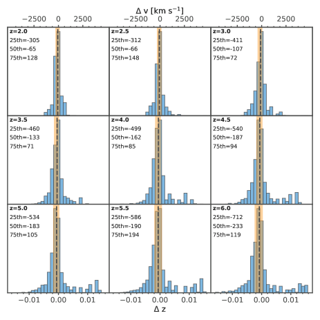
Figure 1: The performance of the systemic error estimation algorithm. The discrepancy for each object in the Monte Carlo simulation is given as $\Delta z$, which is defined as $z_{\mathrm{LASD}}-z_{\mathrm{sys}}$, where $z_{\mathrm{sys}}$ is derived from optical emission lines. The difference in velocities is given on the upper axis. The median value is shown with the dashed black line, and interquartile range (IQR) in the orange region. Median and IQR are also given as inset text, as velocities in km s^-1.

The algorithm recovers $z_{\mathrm{sys}}$ with a median offset of $-65$ km s^-1 at $z=2$, which grows to $-233$ km s^-1 by $z=6$. This is a result of two phenomena: firstly the blue peaks become systematically more suppressed with increasing redshift, because the IGM absorption preferentially removes weaker blue peaks. This causes the algorithm to more frequently switch from two-peak to one-peak mode as redshift increases. Moreover the thicker IGM as $z$ approaches 6 starts to influence the red peak. Damping wings become visible in a minority of simulations, but the blue wing of the red peak becomes systematically more removed, shifting our $z$ estimate to higher positive velocities.

This shift of the estimated $z_{\mathrm{sys}}$ with redshift is both expected and predictable, and we show the redshift evolution of $\Delta z$ in Figure 2.

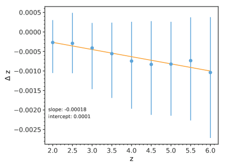
Figure 2: The performance of the $z_{\mathrm{sys}}$ identification with redshift. Redshift is shown on the abscissa, while $\Delta z$ is shown on the ordinate-axis. Each point illustrates the median value from the simulated sample, and the error-bar shows the IQR. Our best fit is a linear function with the coefficients shown in the Figure.

3.3 Matching the spectral resolution

The comparative studies rely upon contrasting high-$z$ spectra for which the spectral resolution is 85–160 km s^-1, with low-$z$ spectra that could in principle have resolutions 5–6 times higher. We first attempt to approximately match the information contents of the spectra, although begin by noting that (a.) the actual difference in resolutions will be much smaller than would be inferred by simply contrasting the instrumental specifications, and (b.) we cannot know the resolution of COS at Ly$\alpha$. This latter point arises because HST/COS has an aperture many times larger than its focused point spread function, and the resolution consequently depends upon the angular size of the source in the dispersion direction. For Ly$\alpha$ emission, this in turn depends upon the size of the galaxy, the effects of Ly$\alpha$ scattering, and the distance. For example: LARS 14 (Hayes et al., 2013, 2014) has half-light diameter in Ly$\alpha$ of $\sim 3.6$ kpc (1.2 arcsec), which is larger than the unvignetted region of the COS aperture; this scale length would reduce the effective resolution from $R\sim 15$,000 to below $R\lesssim 5000$. Yang et al. (2017a) report Ly$\alpha$ full width half maxima of 0.8 ″ for their sample of COS-observed galaxies (most of which are included here), which is exactly the size of the unvignetted region . Henry et al. (2015, whose observations are also subsumed into our sample) use the NUV acquisition images and the line-spread-function (LSF) to estimates spectral resolutions of $\sim 25-46$ km s^-1, but this applies only to the continuum: assuming the linear size of Ly$\alpha$ twice that of the UV on average (Hayes et al., 2013), these numbers would reduce to $\sim 50-100$ km s^-1, which now overlaps with the MUSE range.

For this study, we attempt to obtain a coarse match of spectral resolutions, that will hold for the sample average. For each galaxy we look up $R$ at the wavelength of Ly$\alpha$ from the figures given the Instrument Handbook, and assume a Ly$\alpha$ radius of 0.35 ″ (the median of Yang et al. 2017a). We then compute the smoothing kernel that would be required to match the spectra to $R=3500$ by Pythagorean subtraction. This value is chosen to match the highest resolution possible with MUSE. We finally smooth the COS spectra with this kernel. Again we note that this procedure will not be perfect, but also that any more detailed method would still be limited by the unknown light distribution of Ly$\alpha$ which cannot be known without an extensive imaging campaign.

3.4 Simulating the intergalactic medium absorption

We follow the method described in Inoue et al. (2014), which is based upon statistics of absorption line systems observed in the spectra of quasars at redshifts 3–6. Inoue et al compile observed distribution functions for the column density ($N_{\mathrm{HI}}$) of absorbing systems from Ly$\alpha$ forest (LAF) clouds to damped Ly$\alpha$ absorbing (DLA) systems, along with their evolution with redshift; they then defined a set of power-laws to analytically describe the evolution of the LAF, DLA, and Lyman limit systems (LLS). The column density distribution $dn/dN$ is a steep negative power law, and the redshift evolution $dn/dNdz$ evolves upwards with redshift. With the parameterized PDFs and an assumed target redshift, one can draw random sightlines for absorbing clouds and their column densities.

Any sightline to $z>3$ will encounter a large number of H i clouds that will absorb radiation bluewards of Ly$\alpha$. To apply this absorption, Inoue et al. (2014) adopt the Doppler parameter ($b$) distribution derived from observations of LAF clouds (Hui & Rutledge, 1999; Janknecht et al., 2006), although given the high oscillator strength of Ly$\alpha$ this matters only for absorption at the very lowest column densities. With a sightline of absorbing clouds, each of which has randomly drawn $z$, $N_{\mathrm{HI}}$ and $b$, one can compute the absorption across the whole spectrum: Voigt profiles are used for discrete absorption in Lyman series transitions, while photoionization bluewards of the Lyman would also be needed for the transfer of ionizing radiation. As we are only interested in radiation just bluewards of Ly$\alpha$, only this transition is actually needed for our purposes. We implement the set of equations described in Inoue et al. (2014) so for any sightline we can randomly ascribe an absorption spectrum, which gives IGM throughput as a function of wavelength. In this paper we perform extensive Monte Carlo simulations with this algorithm to statistically study the effect of IGM absorbing clouds on the Ly$\alpha$ profile.

A recent relevant comparison of Ly$\alpha$ emission and absorber statistics has been made by Wisotzki et al. (2018, using the same MUSE-WIDE data as here). They rely mainly upon references included in Inoue et al. (2014), with the addition of Crighton et al. (2015); these authors do revise the DLA incidence rate at $z\sim 5$ somewhat compared to Prochaska & Wolfe (2009), but the incidence rate of proximate DLAs remains negligible compared to lower column density systems that dominate the absorption in the Ly$\alpha$ resonance. Similar approaches have recently been taken by Steidel et al. (2018) using absorber statistics from Rudie et al. (2013), but are optimized to study LyC absorption and do not appear to treat the Doppler parameter independently. The Rudie et al. (2013) statistics anyway appear to be consistent with those of O’Meara et al. (2013) that are used by Inoue et al. (2014).

The statistics of these absorbing populations and their evolution are both completely empirical and very well determined, and the great advantage of absorption selection is that it suffers no redshift bias. The numbers presented by Inoue et al. (2014) will represent a very realistic average absorption in a spatially uncorrelated universe. Note that this implies that the PDFs of the absorbers are treated as being completely independent, and the approach does not account for spatial correlation of matter in the universe. This approach therefore contains no information on the CGM of the target galaxies, or over-densities/clustering around them. On the other hand, galaxies identified by observation will be subject to CGM absorption and may have nearby companion galaxies in the foreground. Thus the regions probed by galaxy surveys may be over-dense on average compared to these IGM prescriptions (entirely randomized absorption). Several authors (Santos, 2004; Dijkstra et al., 2007; Mesinger & Furlanetto, 2008; Iliev et al., 2008; Laursen et al., 2011; Gronke et al., 2020) have discussed the effect of infall and structure local to galaxies, that will enhance the absorption of Ly$\alpha$ because of the increased neutral column crossing $\Delta z=0$. One of the key results of our study is that the excess absorption provided by the CGM is not necessary to explain the evolving Ly$\alpha$ profiles. Since the absorption line statistics are implemented randomly and drawn from Monte Carlo simulations, they provide a lower limit in comparison to absorption in the case of a structured universe. On the other hand, such simulations also neglect the local enhancement of the ionizing background that would be produced by both the observed galaxy and neighboring systems. These sources of ionizing radiation would act in the opposite direction and suppress the local absorption. While we acknowledge the possible discrepancy between the average cosmic absorption and the enhanced opacity that should occur close to galaxies, one of the key findings of this paper is that there is no need for this additional absorption (see Section 6.2).

4 Basic Sample characterization

We present the Ly$\alpha$ luminosity and EW distributions of the two complete samples in Figure 3. The main panel shows the relation between the two quantities, while the vertical histogram above shows the distribution of $L_{\mathrm{Ly}\alpha}$. The two horizontal histograms to the right show the total distribution of $W_{\mathrm{Ly}\alpha}$ in the inner panel, while in the outer panel the COS sample has been restricted to $L_{\mathrm{Ly}\alpha}$$\geq 10^{42}$ erg s^-1; this cut is designed to match the luminosities between the two samples, and is shown by the vertical dashed line in the main figure. The sample matching is discussed in more detail below and in Section 5.3.

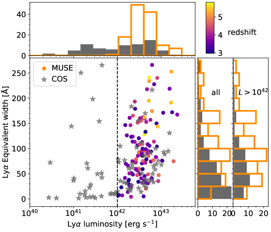
Figure 3: The range of $L_{\mathrm{Ly}\alpha}$ and $W_{\mathrm{Ly}\alpha}$ spanned by the COS sample (grey stars) and MUSE samples (colored circles). The MUSE data are color-coded by redshift, with the colorbar shown to the upper right. A histogram showing the $L_{\mathrm{Ly}\alpha}$ distribution is shown above, and histograms showing $W_{\mathrm{Ly}\alpha}$ are shown to the right: the first includes the total COS sample, while the second shows the COS sample after retaining only galaxies more luminous than the cutoff of $L_{\mathrm{Ly}\alpha}$$>10^{42}$ erg s^-1; this luminosity cutoff is illustrated by the dashed black line.

The range of EWs overlaps well between the sample, spanning values above $\sim 200$ Å, even in the UV-selected low-$z$ sample. The shapes of the EW distribution exhibit similar declines towards higher values, but different behavior in the lowest EW bins: being Ly$\alpha$ selected, the MUSE sample is under-represented at the lowest EWs (0–25 Å) in this binning, while this is the most populated bin the UV-selected COS sample. The two samples are very different in $L_{\mathrm{Ly}\alpha}$: both samples extend to a comparably high luminosity ($\approx 10^{43}$ erg s^-1), but the COS sample extends down to $L_{\mathrm{Ly}\alpha}$ $\approx 3\times 10^{40}$ erg s^-1 while the MUSE data stop at $L_{\mathrm{Ly}\alpha}$$=10^{42}$ erg s^-1. In the high-$z$ study that follows (Section 5.3 and onwards) we retain only the low-$z$ galaxies with $L_{\mathrm{Ly}\alpha}$$>10^{42}$ erg s^-1, so as to match $L_{\mathrm{Ly}\alpha}$ between the samples; this also has the effect of bringing the EW distribution more into agreement (right histogram). First, however, we perform a more general study of the line profiles in the stacked spectra to better understand the origin of the line profiles (blue bumps in particular) and include all COS galaxies so as to preserve the dynamic range in the sample.

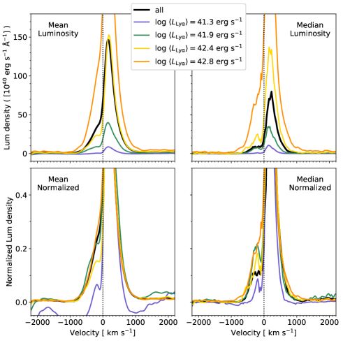
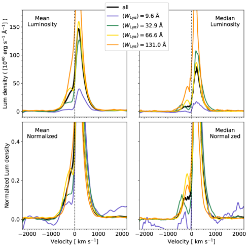
Figure 4: Each panel shows a stacked spectrum from the full sample of galaxies at $z<0.4$ observed with HST/COS. We compare the spectral profiles as a function of $L_{\mathrm{Ly}\alpha}$ (left $2\times 2$ grid) and $W_{\mathrm{Ly}\alpha}$ (right $2\times 2$ grid). The sub-bins, divided by luminosity or EW are color coded with the values shown in the legend, while the total stack of the whole sample is shown in black. In each block of four panels, the left pair shows the mean combination and the right pair shows the median. Upper panels show the spectrum in absolute units of luminosity, while the lower panels show the spectra normalized by the maximum luminosity density, which is always that of the red peak. In the lower panels we zoom in on the luminosity axis so as to emphasize the blue wings.

5 Lyman alpha profiles: results from stacked spectra

The bulk of the data analysis in this paper comes from differential comparison of stacked spectra. Because galaxies lie at different distances we perform the stacking on spectra shifted into the restframe: we divide $(1+z)$ out from the wavelength vectors, and multiply the same factor back in to the flux vectors (always units of erg s^-1 cm^-2 Å^-1) so that the equivalent widths are preserved. We multiply all flux vectors by $4\pi d_{\mathrm{L}}^{2}$ to obtain luminosity density vectors, with units erg s^-1 Å^-1. Every spectrum is then resampled onto the same velocity grid and co-added: we always record both the mean and median spectrum. We note that a well-known limitation of spectral stacking analyses is that by reducing the spectrum to a single number at each frequency, the variations within the sample are lost. This dispersion is re-captured in our case by resampling: when presenting stacked spectra we assess the variation around each average profile by performing a bootstrap analysis of the spectra contained within each bin.

5.1 HST/COS data at $z<0.4$

We show the combined Ly$\alpha$ profiles of the COS sample in Figure 4, where we examine how the profile shape varies as a function of luminosity and EW. It comes as no surprise that when dividing out the sample by $L_{\mathrm{Ly}\alpha}$, galaxies become more luminous (upper plots to the left of Figure 4). We note, however, that there appears to also be some evolution in the blue wing of the Ly$\alpha$ profile in that it appears to become disproportionately stronger in galaxies of higher $W_{\mathrm{Ly}\alpha}$. This becomes much more obvious when the spectra are normalized by the maximum value of the red peak prior to coaddition: in the lower panels to the left of Figure 4 it is clear that as the luminosity decreases, so does the relative contribution of the blue bump, which drops systematically from the orange line (almost $10^{43}$ erg s^-1) to the purple line (100 times less luminous).

We suspect this first result comes from variations in the column of blueshifted absorbing material. There is no absorption from the intergalactic medium at this redshift, and outflows/galaxy winds result in a stronger absorption from interstellar material on the blue side of Ly$\alpha$. This becomes even more marked in the lowest EW bin, where the mean combination reveals true blueshifted absorption of the stellar continuum, and perhaps even a wing from damped absorption extending onto the red side of Ly$\alpha$ at a lower level. At intermediate luminosities, the wing contribution clearly increases from rough 10%, up to 20–30 % for the brightest galaxies.

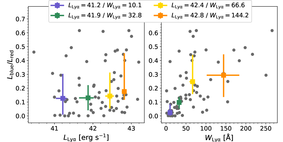
Figure 5: The relative contribution of the blue Ly$\alpha$ peak, expressed as the $L_{\mathrm{B/R}}$ ratio as a function of $L_{\mathrm{Ly}\alpha}$ and $W_{\mathrm{Ly}\alpha}$. It is similar to Figure 4 but on a galaxy-by-galaxy basis. The blue and red Ly$\alpha$ peaks are measured using the LASD software. Colored points are medians with interquartile ranges, and match with the bins in Figure 4.

We examine this trend further in Figure 5, where in grey we show how the blue/red flux fraction contrasts with $L_{\mathrm{Ly}\alpha}$ and $W_{\mathrm{Ly}\alpha}$ for the individual galaxies. Targeting positive blue-side emission only, we only include here galaxies for which the flux density bluewards of line center exceeds zero, and the majority of galaxies from the least luminous bin from Figure 4 are removed. $L_{\mathrm{B/R}}$ shows significant scatter at all luminosities and EWs. Overlaid in color we show the median values for each sub-sample, and encode the interquartile range (IQR) as the shaded region. IQR is a commonly used measurement of dispersion associated with the median representative statistic, including data from the 25^th to 75^th percentiles; for a normal distribution, the IQR is $1.35\sigma$. Attending to the left-most plot, $L_{\mathrm{B/R}}$ appears close to invariant of $L_{\mathrm{Ly}\alpha}$ at the low $L_{\mathrm{Ly}\alpha}$ end, but much of this effect comes from the removal of absorbing galaxies and pure P Cygni-like systems from the bins. In the last bin, however, $L_{\mathrm{B/R}}$ does jump by a factor of $\approx 2$ to 0.34, but overall there is no correlation. However, a tight correlation is seen between $L_{\mathrm{B/R}}$ and $W_{\mathrm{Ly}\alpha}$ (right figure), with Spearman’s $\rho=0.60$, corresponding to $p=7.6\times 10^{-8}$ off 68 data-points. This result is highly significant, and indeed the points show that the lowest EW galaxies have $L_{\mathrm{B/R}}$ at the percent-level, which rises dramatically to $\approx 30$ % at $W_{\mathrm{Ly}\alpha}$ of $\approx 100$ Å. This result quantitatively echoes those demonstrated in Henry et al. (2015) and Yang et al. (2017b), whose Ly$\alpha$ EWs are among the highest observed and whose profiles also include the highest fraction of double peaks. Note, however, that the Henry et al. and Yang et al. observations are subsumed into our sample, and these results are not entirely independent.

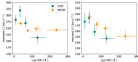
Figure 6: The evolution of the first and second moments of the red peak as a function of $W_{\mathrm{Ly}\alpha}$. The complete range of luminosities of the COS sample are used and shown in green; the MUSE sample, which is more luminous but spans less dynamic range, is shown in orange. Median values and interquartile ranges are shown.

We also note that galaxies with higher $W_{\mathrm{Ly}\alpha}$ also show smaller systematic offsets in velocity (moment 1) and narrower red lines (moment 2), as shown in the normalized median profiles to the lower right left in Figure 4. The second moments of each bin decrease monotonically from 185 km s^-1 at $W_{\mathrm{Ly}\alpha}$ $\approx 30$ Å (shown by both MUSE and COS) to about about 150 km s^-1 at $W_{\mathrm{Ly}\alpha}$ $\approx 230$ Å (probed only by MUSE), as shown in the right panel of Figure 6. We expect this is due to an effect of H i column density in which larger columns result in more Ly$\alpha$ scattering, which reduces the total emitted $W_{\mathrm{Ly}\alpha}$ as the escape probability decreases. This additional scattering further results in broader Ly$\alpha$ lines that are systematically more redshifted.

5.2 VLT/MUSE data at $z>2.9$

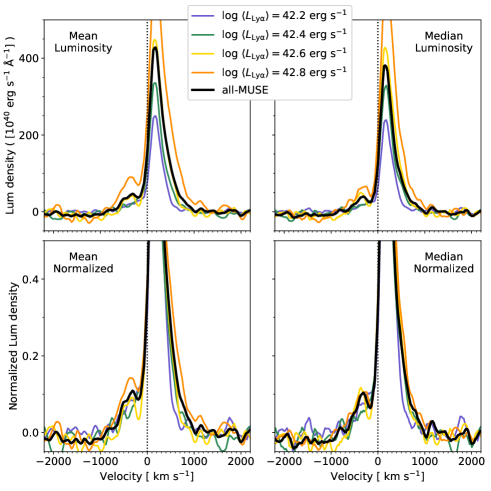
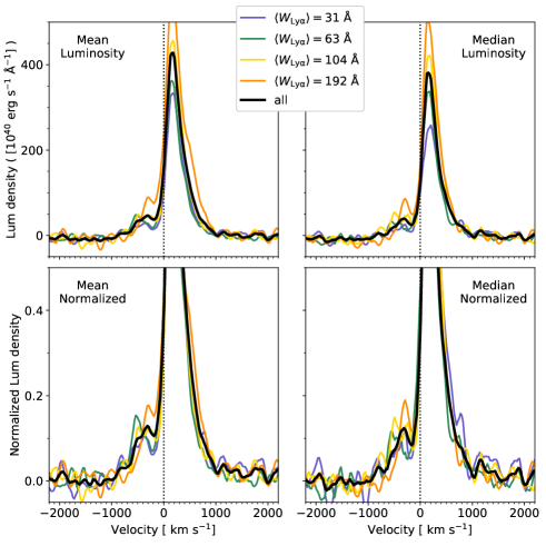
Figure 7: Same as Figure 4, but for the MUSE-WIDE sample, selecting only galaxies at $2.9<z<4$.

Figure 7 shows the stacked spectra obtained with VLT/MUSE. At these redshifts the IGM may have significant influence over the Ly$\alpha$ profile, especially in the blue side, so we temporarily restrict our analysis to $z<4$ galaxies, so as to compromise between studying less absorbed galaxies while still maintaining a significant sample. Blue wings are also visible in the MUSE spectra, and examining all the lower panels of Figure 7 it is clear that some emission is visible to velocities as high as $\Delta v\approx-700$ km s^-1. However unlike the lower-$z$ COS spectra, this blue emission is visible in every bin of luminosity and EW. While the lines are not necessarily in agreement within the noise, relative intensity in the blue bumps does not show a serial decline as it does at lower-$z$: e.g. the green line clearly out-lies the others in the EW comparison, but this is likely attributable to random processes.

In order to explore this lack of a trend further, we perform a bootstrap study using the low-$z$ objects (no IGM absorption), and the IGM simulations described in Section 3.4. We first replace each galaxy in the $2.9<z<4$ MUSE sample with the low-$z$ galaxy that has the closest $L_{\mathrm{Ly}\alpha}$. We then randomly draw a sightline through the IGM to the MUSE redshift, attenuate the COS galaxy, and bin and stack this random sample. We examine the frequency with which a statistically significant ($p<0.05$) trend is recovered. With samples the size of this MUSE subset ($N=74$) the correlation is almost never reproduced: with just a few percent of realizations showing significant correlations. However when we artificially increase the bootstrap simulation to include $\approx 1000$ objects (including galaxies more than once but with different random IGM sightlines) the trend does re-emerge, with the $L_{\mathrm{B/R}}$ ratio reduced by a factor of 2 compared to $z=0$. This is exactly what would be expected for large samples, as the stochastic effect of the IGM is smoothed out over a large number of realizations.

In principle this method could be used to calculate the necessary sample size required in order to statistically study these trends at high-redshift, but many other factors will hold influence over the result. For example the precise recovery will also depend upon the signal-to-noise ratio of both the high-$z$ data and the low-$z$ data we use to simulate it, and the result will also be redshift dependent. Nevertheless we proffer the advice to use low-$z$ data from the extensive and growing HST archives to realistically simulate the recovery of high-$z$ Ly$\alpha$ spectral profiles in large samples.

Interestingly, the same trend in the width and offset of the red peak is observed in these higher-$z$ systems, as discussed for $z=0$ galaxies in Section 5.1. The normalized profiles of Figure 7 (lower left) both show the lower-$W_{\mathrm{Ly}\alpha}$ galaxies to have both broader and less shifted red profiles; same is shown quantitatively in the right panel of Figure 6. Hashimoto et al. (2015) show the red-peak velocity shift to be much higher in LBGs than in LAEs using optical line emission such as H$\alpha$ and [O iii], and similar effects are probably at work here. They attributed this effect to radiation transfer effects where the LBG column density is higher, using RT modeling in spherical shells. Cassata et al. (2020) also show similar effects using the [C ii] 158 µm line: they show weak correlations of Ly$\alpha$ redshift with UV magnitude, stellar mass and SFR. These go in the direction that would support the hypothesis that mass drives the trend, but none of Cassata et al’s trends reach statistical significance, possibly because of dynamic range.

5.3 Comparison of matched samples

The COS sample from low-$z$ is needed for an estimation of the intrinsic Ly$\alpha$ line profile. However, to produce such an intrinsic, IGM-free template for the high-$z$ galaxies, we would ideally match the samples in their SFRs, masses, compactness, dust optical depths, ionizing intensities, etc. Such sample matching is far in the future and the huge majority of this information is unavailable at $z>2.9$; obtaining it will require extensive surveys with the James Webb Space Telescope (JWST). We instead make the most basic compromise, and take only COS galaxies that overlap with the MUSE sample in the two key observables, of $L_{\mathrm{Ly}\alpha}$ and $W_{\mathrm{Ly}\alpha}$. The distribution of these quantities is shown in Figure 3, where the full COS sample extends to 30 times lower luminosities than the faintest MUSE-WIDE system. This is certainly to be expected when contrasting distant Ly$\alpha$-selected galaxies with nearby UV-selected systems.

We impose a cut in the Ly$\alpha$ luminosities at $10^{42}$ erg s^-1, as shown by the dashed line in Figure 3. We do not aim to accurately reproduce the distributions in $W_{\mathrm{Ly}\alpha}$ and $L_{\mathrm{Ly}\alpha}$, but note a number of similarities. Firstly the upper envelope of the luminosity histogram is well-matched between the samples. In the $W_{\mathrm{Ly}\alpha}$ histograms, the MUSE-WIDE survey is skewed towards somewhat higher values, with a median $W_{\mathrm{Ly}\alpha}$ of 78 Å compared with 61 Å for the low-$z$ sample. The Ly$\alpha$ blue/red flux ratio depends strongly upon $W_{\mathrm{Ly}\alpha}$, and increases towards higher EWs as also shown in Figure 5, and this effect could introduce a bias in the direction that high-$z$ galaxies have larger intrinsic blue/red ratios. While we do not see the same behavior in the high-$z$ galaxies directly, we showed this to result from the stochastic IGM absorption in Section 5.2. On the other hand, the median EWs of the two samples remains close (much smaller than the interquartile range), and while acknowledging the EW difference could introduce a bias we expect it to be a minor one.

We finally note that the COS aperture (radius of 1$\farcs$25) samples only a projected distance of 5 kpc at $z=0.25$, and should part of the line profile be built from extended emission then that would obviously not be captured by the low-$z$ observation. Indeed Leclercq et al. (2020) do find differences in the velocity centroids of Ly$\alpha$ profiles extracted from the core and halo regions, with the implication that asymmetric profiles are built from differences between the core and halo (see also Erb et al., 2018). However we note that these conclusions from the deep MUSE data were drawn from a sub-sample in which the halo flux fraction was high by construction, skewing the interpretations in the direction of the more luminous and extended LAEs.

In the coming Section on redshift evolution, we use the COS sample to estimate the intrinsic and absorbed Ly$\alpha$ line profile from high-$z$. From now on, however, we take only low-$z$ galaxies from the luminosity matched sub-sample ($N=45$).

6 The Co-Evolution of Lyman alpha profiles and the intergalactic medium

In this Section we present our main results concerning the evolution of the Ly$\alpha$ emission line with redshift and how we can explain this in terms of the co-evolution of galaxies and the IGM.

6.1 The Redshift Evolution of the Ly$\alpha$ Profile

We now proceed to study the redshift evolution of the Ly$\alpha$ profile, using differential stacking comparisons similar to those already shown. We bin the sample in redshift into five sub-samples, and show the results in Figure 8 with sample medians and half-quartile ranges shown in the caption. The high-$z$ galaxies from the MUSE-WIDE survey are always shown in color, and the $z\approx 0.25$ sample, with no IGM, in black. For the low-$z$ sample, we adopt precisely the same strategy as in Section 5.1, except switch the estimate of $z_{\mathrm{sys}}$ from the measured value to that estimated from the Ly$\alpha$-line using the LASD algorithms. This ensures consistency in the treatment of the samples. Despite changing the $z_{\mathrm{sys}}$ estimator, the COS profiles remain very similar, and the black line in Figure 8 is close to the average of the yellow and orange lines in the lower left panels of Figure 4. Especially for the more luminous galaxies, the errors on the recovered systemic redshifts become comparable with the resolution of the spectrograph.

At each redshift we resample the galaxy bin using bootstrap techniques. We randomly re-draw a sample of the same size and recompute the mean and median; iterating this over 1000 realizations we compute the variations of each stacked subsample about the true mean and median. For mean profiles we show the central 68^th percentiles, and for the median profiles we show the interquartile range.

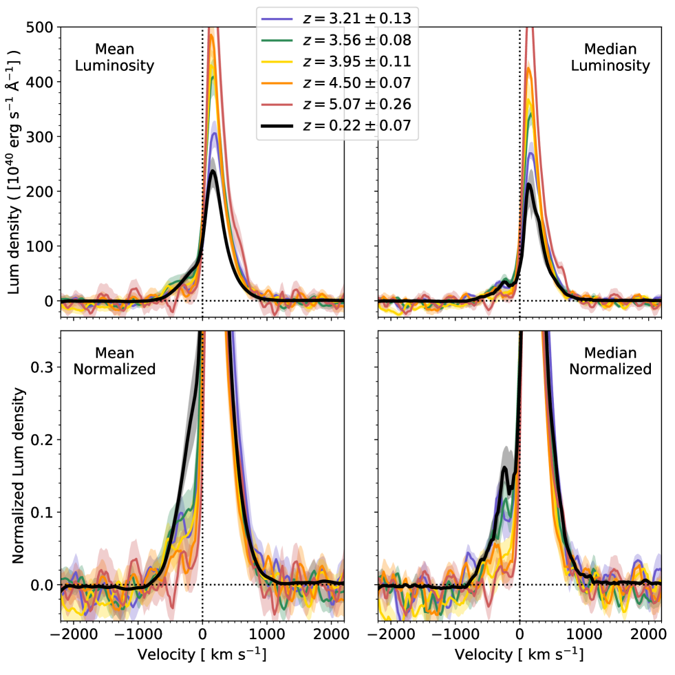
Figure 8: The evolution of the Ly$\alpha$ profile with redshift. The individual panels are the same as in Figures 4 and 7, but the sample is now binned by redshift; each bin includes 45 or 46 galaxies. The MUSE-WIDE sub-samples are shown in colors and the redshifts are displayed in the caption. The low-$z$ sample observed with HST is shown in black. Error regions are shaded, and represent the interquartile range estimated from bootstrap resampling. The evolution of the blue wing, decreasing with increasing $z$, is obvious.

Several effects are clear from Figure 8. Among the most obvious, visible in the upper two panels there is a trend among the MUSE wide galaxies to become more luminous with increasing $z$. This is the well-known Malmquist (1922) bias, that manifests as the most luminous systems being preferentially detected. In this instance it results from the luminosity distance increasing with $(1+z)$ faster than the sensitivity of MUSE decays with $(1+z)\times\lambda_{\mathrm{Ly\alpha}}$: even though the Ly$\alpha$ luminosity function is close to constant across this redshift range (e.g. Herenz et al., 2019), there is a upwards evolution the sample luminosities because only the most luminous subset of the respective galaxy population is detected at highest redshifts.

Blue wings are visible in the profiles. This is most abundantly clear in the COS profiles from low-$z$, but sub-dominant blue wings are visible in the un-normalized profiles (upper). However their intensity evolution goes in the opposite direction from the evolution in the red peaks: the highest intensity blue peaks are found among the $z\approx 3-4$ subsamples, and the $L_{\mathrm{B/R}}$ ratios decrease with $z$. This is more noticeable when we normalize the profiles, which we show in the lower two panels. Here we zoom in to visualize the blue peaks: attending mainly to the median stack (lower right) the $z\approx 3-3.5$ sub stacks show normalized intensity of 10 %, which drops further to about 5 % by $z\approx 4$ and almost to zero at $z=4.5$ and up.

In light of the Malmquist bias discussed above, a natural question becomes whether this evolution in the line profiles may result from selection effects or evolution with luminosity. This phenomenon is seen within the IGM-free COS sample (Figure 4) but not in the MUSE sample (Figure 7), and we showed with simulations (Section 5.2) that it would be impossible to detect for the given sample size and spectral quality even at $z=3-4$. Importantly, the median luminosity evolution due to the Malmquist bias is only a factor of 2 between $z=3$ and 5.5, which is significantly smaller than the difference between the bin median in Figure 4 where the trend is seen. We conclude that the blue peak evolution presented in Figure 8 is not attributable to selection effects of this kind.

Another potential source of bias could be the errors on the estimated $z_{\mathrm{sys}}$: these errors increase with redshift (Figure 2), and higher errors at $z\sim 5-6$ could artificially suppress the blue peaks. We have tested the impact of these increasing $z_{\mathrm{sys}}$ errors by adding an additional error term to the redshifts of the lower-$z$ galaxies: we compute this from the fit in Figure 2, and derive the magnitude of the random deviate needed to match the breadth of the distribution at $z\approx 6$. We find no significant effect on the profile evolution.

The COS spectrum from $z\approx 0.25$ shows a $L_{\mathrm{B/R}}$ ratio of $\approx 16$ % in the median stack, and higher still in the mean. Mean stacks, however, will always be dominated by the more luminous systems at a given velocity, and result in line profiles that are on average less representative of a given galaxy. We observe a reduction in the normalized blue peak intensity of about $\approx 60$ % to $z=3$; from a simple by-eye analysis we would estimate the an IGM opacity of $\tau_{\mathrm{IGM}}^{\mathrm{blue}}$$\approx 0.45$ from Figure 8. In the coming Section we perform a more detailed study of this.

6.2 The Impact of the IGM

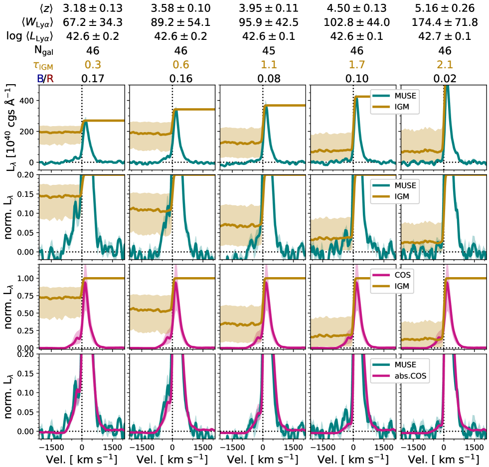
Figure 9: Simulating IGM absorption of LAEs at various redshifts. Each column shows a different redshift bin: the median $z$, $W_{\mathrm{Ly}\alpha}$, $L_{\mathrm{Ly}\alpha}$  are listed above, together with the half-quartile range of each quantity, and the number of galaxies in each bin. The top rows show the median stack of the Ly$\alpha$ luminosity density in absolute units (erg s^-1 Å^-1) in green, with the median IGM absorption overlaid, scaled so that 1 matches the red peak of the Ly$\alpha$. Shaded regions represent the interquartile range. The second row shows the same Ly$\alpha$ profiles normalized to an intensity of 1 at the peak, and zoomed in around the wings of the line: IGM is again shown on arbitrary scale of $0.15\times$. The third row shows the intrinsic spectrum in pink, which is simulated from an equal number of galaxies drawn from the luminosity- and EW-matched samples from $z\approx 0$. This spectrum is always normalized to a peak intensity of 1, and the shaded region shows the quartile range derived from bootstrap simulations (see Section 6.2 for details). The IGM transmission is also shown in the third row

, now scaled to the absolute throughput. The average optical depth, $\tau_{\mathrm{IGM}}^{\mathrm{blue}}$, is computed in the $\lambda_{\mathrm{rest}}=1200-1210$ Å range, and is shown at the top of each column. The lowest row shows the profile of the COS spectrum, absorbed by the IGM for each redshift bin, together with the stacked observed MUSE spectra for the same redshift. The overlap between the two lines is often striking.

The COS spectra are not susceptible to intergalactic Ly$\alpha$ absorption: the IGM optical depth at $\lambda=1200-1210$ Å is $\tau_{\mathrm{IGM}}^{\mathrm{blue}}$ $\lesssim 10^{-6}$. Thus if the Ly$\alpha$ line profile observed in the COS sample is representative of the profile emergent from the CGM at redshifts beyond 3, this empirical spectrum will serve as a template. We restate that we selected the low-$z$ sample to match the observables of the MUSE-WIDE sample in both Ly$\alpha$ luminosity and EW (Figure 3), which argues in favor of this utilization.

We present our findings on the redshift evolution of the Ly$\alpha$ profiles, together with simulations of the evolving IGM opacity, in Figure 9. Each column shows data and simulations for a different redshift bin, and is headed with the following: redshift, $W_{\mathrm{Ly}\alpha}$, $L_{\mathrm{Ly}\alpha}$, the number of galaxies in the bin, $\tau_{\mathrm{IGM}}^{\mathrm{blue}}$, and the $L_{\mathrm{B/R}}$ ratio from the MUSE-WIDE stacks. The left column shows the results from the lowest redshift, centered at $z=3.18$. The average Ly$\alpha$ profile from the stack of 46 high-$z$ galaxies is shown in the top row (this is the same as the red spectrum in Figure 8). At this redshift the blue wing is very clear, and is visible out to velocities of $-700$ km s^-1; this is especially clear in the second row, where we zoom in to show the blueshifted emission in detail. The IGM throughput ($I/I_{0}$) is shown in yellow in various rows: in the top two panels it is arbitrarily scaled, while in the third row it is presented in absolute throughput: in the first column, the average transmission just bluewards of Ly$\alpha$ is $\approx 0.75$, corresponding to the $\tau_{\mathrm{IGM}}^{\mathrm{blue}}$ $=0.3$ quoted in the heading.

The third and fourth rows show the simulated Ly$\alpha$ profile (pink lines) at each redshift, in the unabsorbed and absorbed cases, respectively. We simulate the emergent Ly$\alpha$ profile using a randomly drawn sub-sample of $z\approx 0$ spectra, taking $N$ COS observations, where $N$ is the number of high-$z$ galaxies in the bin (46 in this example). For this we consider only the luminosity and EW-matched subsamples (Section 5.3 and Figure 3). Assuming no evolution in the intrinsic Ly$\alpha$ profiles, we first normalize and median-combine the $N$ low-$z$ spectra, using the same routines as for the MUSE data. We finally run a 1000-realization Monte Carlo simulation to build the distribution of expected profiles around this median (IQR is shown as the shaded region). This unabsorbed spectrum is shown in the third row of Figure 9.

For each galaxy discussed above, and in every realization of the Monte Carlo simulation, we also add the effect of the IGM by artificially absorbing each selected COS spectrum. Prior to normalization, we multiply each spectrum by an absorption spectrum, randomly generated for a single sightline through the IGM to the redshift of the MUSE spectrum (see Section 3.4 for details). We then proceed with the normalization, co-addition, and distribution sampling in precisely the same way as for the unabsorbed spectra in the previous paragraph. The resulting median spectrum, together with its quartile range, is shown by the pink line in the bottom row of Figure 9; the average high-$z$ spectrum is again shown in green. Attending again to the lower left panel ($z=3.18$), the agreement between the simulated spectrum and the observed spectrum at the same redshift is striking. The normalized flux goes to zero in the blue wing at velocity offsets of $\lesssim-700$ km s^-1 in both spectra; immediately bluewards of line-center they differ by $\approx 20$ % in normalized intensity, with the simulated absorption from the IGM marginally over-predicting the observation from $z\sim 3$.

It is possible that this slight deficit in Ly$\alpha$ flux at $\Delta v\gtrsim-300$ km s^-1 is due to enhanced absorption from structure/galaxies adjacent to the target LAEs. The IGM simulations follow the prescription of Inoue et al. (2014), which is constructed using the observed distribution of H i-absorbing systems identified along the sightlines to luminous quasars. Each absorber is drawn at random from a probability distribution function, and is therefore independent of all other absorbing systems and the target galaxy itself; it neglects the galaxy-galaxy spatial correlation and the fact that these LAEs should occupy somewhat over-dense regions which will enhance the absorption within the volume bound from the Hubble expansion by gravity. Precisely this has been addressed in various numerical methods (Santos, 2004; Dijkstra et al., 2007; Mesinger & Furlanetto, 2008; Iliev et al., 2008; Laursen et al., 2011; Gronke et al., 2020), who have all used cosmological hydrodynamical simulations to assess the distribution and velocity field of material within 10 Mpc of galaxies. In fact, such simulations have already been used to correct the Ly$\alpha$ EW in spectroscopic studies of high-$z$ galaxies (Pahl et al., 2020). While the precise results will depend somewhat upon the details of the simulation and mass ranges probed by the observation, the broad picture is clear: at $z\approx 3-3.5$ sample there is a sharp excess of Ly$\alpha$ absorption at velocities $\approx-50$ to $-100$ km s^-1 from line-center that increases the Ly$\alpha$ absorption by a factor of two to three times. This excess of absorption returns to the baseline value (random absorption systems) at velocity offsets exceeding $\approx 300$ km s^-1, and it seems entirely plausible that this phenomenon could explain the deficit of blue-side flux close to line-center at the lower redshift end of the MUSE sample. However, we note while this excess absorption due to circumgalactic material is visible for all halo masses at $z\gtrsim 3$ in the simulations, it is not required to explain the stacked spectra studied here.

We now proceed to examine the next redshift bin, centered at $z=3.55$. The MUSE-WIDE galaxies at this redshift completely match with those of the previous bin in $L_{\mathrm{Ly}\alpha}$; and the median EWs are consistent within 8Å ($\approx 25$ % the half-quartile range; values quoted above the figure rows). By this redshift the IGM optical depth has increased by a factor of two (0.3 to 0.6) and provides significantly more absorption on average. When we use this IGM absorption profile to artificially attenuate the COS spectrum we bring the COS and MUSE blue components into tight agreement at all velocities between $-1000$ and 0 km s^-1. Indeed the absorbed COS spectrum completely overlies the MUSE stack, with no need for excess absorption at any velocity; it is difficult to tell which stack is which.

The IGM opacity increases systematically, with $\tau_{\mathrm{IGM}}^{\mathrm{blue}}$ going from 1.1, to 1.8, to 2.3 at redshifts $z=3.9$, 4.5, and 5.4, respectively. If we take the typical $L_{\mathrm{blue}}/L_{\mathrm{red}}$ ratios observed at low-$z$ as representative ($\sim 0.35$; Figure 5), then we would expect the blue bumps to reach approximately 0.1, 0.06, and 0.03 in the absorbed spectra that are normalized to the red peak. This is precisely what is shown in columns 3, 4, and 5 of Figure 9: probable blue bumps remain but if real their significance is low, and their normalized intensity is reduced to the level of a few per-cent. At none of these higher redshifts do we need an additional component of absorption at low blueshifted velocities, that we attributed to structure near to the galaxies or cosmic infall (e.g. Dijkstra et al., 2007; Laursen et al., 2011).

7 Discussion and Implications

7.1 Radiation Transfer Simulations in Realistic Environments

In recent years a number of theoretical efforts have been devoted to predicting the Ly$\alpha$ output of galaxies from RT models, using two complementary approaches. Researchers have used idealized model galaxies described by a number of single parameters (gas column density, outflow velocity, etc) to examine how Ly$\alpha$ profiles vary with these basic properties (e.g. Verhamme et al., 2006; Schaerer et al., 2011; Gronke & Dijkstra, 2016): the main criticism levelled at these studies is that realistic galaxies are not well described by such simplistic models, so the community instead turns to simulated galaxies to produce the manifold for RT simulations (e.g. Tasitsiomi, 2006; Laursen & Sommer-Larsen, 2007; Faucher-Giguère et al., 2010; Zheng et al., 2010; Barnes et al., 2011; Trebitsch et al., 2016; Smith et al., 2019). These models are not without criticism either, and are often cited as having insufficient spatial resolution, particularly at CGM scales, to capture the representative geometry for the RT. RT in these settings almost invariably over-produces Ly$\alpha$ emission on the blue side of line center, at a level that is only very rarely found by observation. The proponents frequently appeal to intergalactic absorption to remove the blue component, but our results show that this appeal is unlikely to be realistic. The uncorrelated Ly$\alpha$ absorbing systems do not reach sufficient opacity to universally suppress the blue emission seen in starburst galaxies, and we find no need within this large dataset for an excess opacity near galaxies. However, we also note that LAEs such as these do reside in lower-mass halos, and there still may be room for the effect to be more prominent on sightlines towards higher halo mass.

7.2 Is there still space for excess opacity?

The absence of enhanced Ly$\alpha$ within a few hundred km s^-1 of the galaxies is worthy of further discussion. One explanation could be that with structure building up hierarchically over time, we need to wait until redshifts $\sim 3$ for significant neutral gas to affect the Ly$\alpha$ line to an extent greater than the uncorrelated cosmic average. One may speculate that the galaxies studied here are less massive than those studied in the simulations referred to above, and the amplitude of their over-density/infall compared to the cosmic mean will be lower. However with the typical range of stellar masses in the mock galaxies being $\approx 10^{7}-10^{10}$ M_⊙ this seems unlikely on average as LAEs of this luminosity probably have $M_{\mathrm{stell}}\approx 10^{8}-10^{9}$ M_⊙. Alternatively, the gas may be more ionized than thought, which would imply the simulated opacity is overestimated. This might be due to a lower clumping factor of cold, neutral material (e.g., because of a lack of spatial resolution; van de Voort et al. 2019; Hummels et al. 2019) or additional ionization sources. We may point towards photoionization of low-mass companion structures by the enhanced UV background close to early galaxies, where the excess UV results from numerous galaxies that are too faint to be detected. Such galaxies may, however, be visible in the ultra-deep MUSE pointings (e.g. Bacon et al., 2017).

We also question whether this absence of excess blue-side absorption could be the result of a conspiracy of parameters, where the intrinsic $L_{\mathrm{B/R}}$ does increase with $z$, but is suppressed by absorption on small scales. Indeed the Malmquist bias results in an upwards evolution of $L_{\mathrm{Ly}\alpha}$ with $z$ (Figure 8, upper) which may be expected to increase the intrinsic $L_{\mathrm{B/R}}$ (Figures 4 and 5). However we note that the trends that are revealed in the COS sample are manifested over a dynamic range of almost 2 dex, whereas the overall evolution introduced by the Malmquist bias is just a factor of 2 between $z=3$ and 5.5. In fact, attending to the sample medians shown at the top of Figure 9, there is very little evolution in total (observed) $L_{\mathrm{Ly}\alpha}$. So while we cannot rule out a conspiracy of parameters, we believe the dynamic range, coupled with the relatively small Malmquist bias, are insufficient to produce an effect of the required magnitude.

7.3 Less blueshifted Ly$\alpha$, but more Ly$\alpha$ overall

We note also that this downwards evolution of the blue contribution, and clearly increasing impact of the IGM, occurs against the backdrop of an overall increasing Ly$\alpha$ output from the galaxy population. This is shown by numerous lines of evidence including a Ly$\alpha$ fraction among LBGs that increases significantly over the same redshift range we probe here (Stark et al. 2010; Cassata et al. 2015; De Barros et al. 2017, although see also Caruana et al. 2018), an increase in the volume-averaged Ly$\alpha$ escape fraction of galaxies (Hayes et al., 2011; Dijkstra & Jeeson-Daniel, 2013; Konno et al., 2016; Wold et al., 2017), and the increasing agreement of the UV LFs of LAEs and LBGs (Ouchi et al., 2008). In these first papers we could only speculate about the actual influence the IGM has on the Ly$\alpha$ emission: because the Ly$\alpha$ output increases with $z$, we concluded the IGM could not act to strongly suppress Ly$\alpha$. The new evidence presented here shows that this is not the case, and if the COS-measured $L_{\mathrm{B/R}}$ of $\approx 0.35$ continues to hold at high-$z$ (or even grow), then the IGM removes an additional quarter of the total Ly$\alpha$ (integrated over the whole line) at $z=5.5$ compared to 3. The implication is that the Ly$\alpha$ emitted from galaxies must increase by a corresponding amount over the same redshift range in order to counteract this effect. Such excess emission may be attributed to the decreasing dust content, stellar metallicity, or average age of galaxies with redshift, implying they must evolve even faster than previously claimed (e.g. Hayes et al., 2011).

7.4 Implications of the evolving ISM and ionizing output of galaxies

The blue/red flux ratio is often invoked as a tracer of the interstellar medium of galaxies, especially regarding the H i column (e.g. Erb et al., 2016) and ionizing output (e.g. Verhamme et al., 2015). The absence of strong evolution in the intrinsic $L_{\mathrm{B/R}}$, therefore, raises the question of whether the ionizing escape fraction ($f_{\mathrm{esc}}^{\mathrm{LyC}}$) is constant between $z=0$ and $z=6$. While we do not have the data necessary to answer this question directly, it is likely that $f_{\mathrm{esc}}^{\mathrm{LyC}}$ does not change dramatically within the samples analyzed here. However these samples comprise a different fraction of the galaxy population at each redshift.

Steidel et al. (2018) studied the LyC output of a large sample of UV-selected galaxies at $z\sim 3$, and determined that the highest escape fractions are found among galaxies with higher $W_{\mathrm{Ly}\alpha}$. Moreover, these same higher $W_{\mathrm{Ly}\alpha}$ galaxies also show more Ly$\alpha$ emission close to $\Delta v=0$ than weaker/non-emitting galaxies, which is consistent with our own results here at $z\lesssim 0.4$ (Section 5.1). It is likely that the Ly$\alpha$ selection of our sample, combined with the somewhat fainter UV continuum magnitudes would place our galaxies towards the upper end of the $f_{\mathrm{esc}}^{\mathrm{LyC}}$ distribution, at approximately $f_{\mathrm{esc}}^{\mathrm{LyC}}$ $\sim 20$ %. The same $f_{\mathrm{esc}}^{\mathrm{LyC}}$ conclusion would also hold in the $z\gtrsim 5$ sample, but note that LAEs comprise a larger fraction of the total galaxy population at this higher redshift (e.g. Ouchi et al., 2008; Stark et al., 2010, and arguments in Section 7.3). If anything, our result of non-evolving line profiles would lend support to a picture in which the volume-averaged ionizing output of galaxies evolves in line with the Ly$\alpha$ fraction and/or the evolving Ly$\alpha$ luminosity function.

Here we also recall that the average $f_{\mathrm{esc}}^{\mathrm{LyC}}$ required to reionize the universe must be on this order (Robertson et al., 2015); while it may be somewhat lower (e.g. Finkelstein et al., 2019) it cannot be much higher as it would violet the ‘photon-starved’ nature of reionization (e.g. Bolton & Haehnelt, 2007). By the same token, the average $f_{\mathrm{esc}}^{\mathrm{LyC}}$ at the lower redshift end of our MUSE sample ($z\sim 3$) must occupy the same range so as not to over-heat the Ly$\alpha$ forest (Becker & Bolton, 2013).

A claim of an average $f_{\mathrm{esc}}^{\mathrm{LyC}}$ of $\sim 20$ % at $z\sim 0$ would indeed be suspicious, as LyC emission is rarely reported in the more general starbursting galaxy population (Leitet et al., 2013). It is only in the last few years have LyC detections have systematically been made (e.g. Izotov et al., 2018); while the $f_{\mathrm{esc}}^{\mathrm{LyC}}$ estimates are again comparable (10–20 % on average but with large dispersion) these measurements derive from samples of specially selected, rare compact starbursts with highly ionized ISM. We again caution that the fraction of strong Ly$\alpha$-emitting galaxies at these redshifts is an even smaller fraction of the population than at $z\sim 3$ (e.g. Cowie et al., 2010).

8 Outlook and limitations

In Section 4 we showed that there is real and strong evolution in the relative contribution of the blue wing of the Ly$\alpha$ emission with redshift, and in Section 6.2 that we are able to fully reproduce this with IGM absorption. The main assumptions were that the intrinsic Ly$\alpha$ spectrum is invariant with redshift and can be described by the profile of low-$z$ sample observed with HST/COS, and that the IGM is spatially uncorrelated and does not require an enhancement from companion galaxies/proximate Lyman limit systems. Furthermore the remarkable agreement between the Ly$\alpha$ profiles at all $z$, supports the utility of our improved heuristic $z_{\mathrm{sys}}$ estimation from analysis of the Ly$\alpha$ line profile (Runnholm et al., 2020a), despite an evolution in the IGM opacity ($\tau_{\mathrm{IGM}}^{\mathrm{blue}}$) of more than two optical depths. This naturally raises the question of to what extent the observed evolution of the Ly$\alpha$ profile can be used to infer the IGM opacity at even higher redshifts, and into the epoch reionization (EoR).

As mentioned in Section 1 strong blueshifted emission peaks have also been found at $z=5.8-6.6$. Some prime examples include Aerith B at $z=5.8$ (Bosman et al., 2020), NEPLA4 at $z=6.5$ (Songaila et al., 2018) and COLA1 at $z=6.6$ (Hu et al., 2016; Matthee et al., 2018), which all show spectacular Ly$\alpha$ profiles, with dominant red lines but inarguable blue peaks. Songaila et al. (2018) suggest that such spectral features may be present in the profiles of less luminous galaxies in significant numbers of up to 1/3. This is quite unexpected in light of the results shown in Figures 8 and 9, but two key points must be born in mind when co-interpreting the datasets. Firstly our analysis is based upon stacking which acts as a lossy compression that removes all information concerning the dispersion within the sample. If blue bumps are present at $z>5$ in the galaxies from the Urrutia et al. (2019) data release, as a significant minority, they will not be represented in the median stacking (right columns) and will be hard to detect in the averaging. Secondly the $z>5.7$ blue-bump objects mentioned above are all significantly more luminous than MUSE-WIDE galaxies: typical log ($L_{\mathrm{Ly}\alpha}$/(erg s^-1)) is 43.5, while our $z\approx 5.2$ subsample has a median luminosity that is 0.8 dex lower.

As we are likely unable to identify blue bumps in the MUSE-WIDE data, this makes comparison to the more luminous systems difficult. For a fixed Ly$\alpha$ escape fraction, the ‘ordinary’ systems studied here would themselves be almost ten times less ionizing than the luminous blue-bump galaxies. Nevertheless, the overwhelming majority of the ionizing photons required to ionize a bubble with radius at least 1 Mpc come from sources other than the galaxy itself, even for more luminous galaxies (Bagley et al., 2017), we should be wary of over-interpreting spectra of single galaxies. Even in the case of very large H ii regions, the presence/absence of blue peaks/wings may have more to do with the galaxy’s position along the line-of-sight with respect to the bubble edges, and the details of its ISM, than with the IGM state.

One limitation of our study is that our galaxies are Ly$\alpha$-selected. At the higher ends of mid-$z$ ($z\sim 4-5.5$) this may remain a representative sample of the galaxy population: the average Ly$\alpha$ output of galaxies continually increases (Stark et al., 2010; Hayes et al., 2011). However all these Ly$\alpha$-quantities begin to drop after $z\sim 6.5$ (Schenker et al., 2012), which raises doubts about the utility of LAE-based probes at higher redshifts. At these redshifts the Ly$\alpha$-based studies may provide representative statistics about the geometry of H ii bubbles, but not about the regions between, which must still be probed with (most likely) UV-selected/Lyman break galaxies.

In the coming years, Subaru Prime Focus Spectrograph (PFS) will embark upon very large area Ly$\alpha$ surveys (14 deg² under the Subaru Strategic Program) targeting UV-selected galaxies over what is likely to be the complete range of bubble distributions in the EoR. PFS can target Ly$\alpha$ at $\lesssim 6.3$ at $R\approx 5000$ with the mid-resolution red spectrograph, and at $\gtrsim 6.7$ at $R\approx 4300$ with the NIR spectrograph; the gap between the two redshifts can be filled by the low-resolution red spectrograph at $R\approx 3000$, which is comparable to MUSE at these redshifts. An obvious study therefore becomes the behavior of the Ly$\alpha$ profile as a function of local galaxy environment, in which the blue contribution to the total Ly$\alpha$ can be used to constrain the dispersion on $\tau_{\mathrm{IGM}}$ at fixed redshift. This paper, and Figure 9 in particular, shows that this goal can be reached at the expected resolving powers of PFS.

The natural drawback of this fiber-fed approach, of course, is that it demands photometric pre-selection, and will not have the possibility to identify new LAEs within its own observation. The SSP will target LBGs and LAEs from SSP imaging surveys GOLDRUSH and SILVERRUSH, and as a consequence the Ly$\alpha$-emitter components will be limited to the narrowband depths, which currently fall around log ($L_{\mathrm{Ly}\alpha}$/(erg s^-1)) = 43.0 for SILVERRUSH (Konno et al., 2018). Thus the survey will deliver huge numbers of spectra with luminosities close to those of COLA1 and NEPLA4, and LBGs from GOLDRUSH that are more massive still, it remains unclear how well the survey will sample the mass range of more ‘normal’ star-forming LAEs at similar redshift. Thus the observational necessity remains for deep IFU studies with instruments like MUSE, that deliver 100% spectroscopic completeness with the contrast and depth that can only be provided by spectroscopic surveys.

9 Summary and Conclusions

We have undertaken an extensive study of the Ly$\alpha$ emission line profile from star forming galaxies at various cosmic epochs, using some of the largest samples of available spectra obtained with HST/COS at low-$z$ and VLT/MUSE at $z=2.9$ to 6.6. Our main findings can be summarized as:

• We see distinct and predictable variations in the shape of the Ly$\alpha$ profile in the low-$z$ sample. The blue peak gets stronger with increasing $W_{\mathrm{Ly}\alpha}$. We believe this trend results from atomic gas column being the dominant factor in regulating Ly$\alpha$ output, and as the galaxies almost certainly have outflows the blue peak is more significantly suppressed than the red.

• This trend is not observed within the MUSE sample at $z=2.9-4$ ($N=74$ galaxies). Using Monte Carlo bootstrap simulations of the IGM opacity and applying them to the low-$z$ sample, we show that the stochastic nature of IGM opacity to Ly$\alpha$ is entirely sufficient to remove trends of this amplitude.

• We find the red component of the Ly$\alpha$ profile becomes broader and increasingly redshifted at lower Ly$\alpha$ equivalent widths. We attribute these effects to the covering of atomic material. More scattering increases the absorption of Ly$\alpha$ and preferentially in the blue wing while, at the same time, the larger column density requires longer frequency excursions to escape, resulting in broader, more redshifted lines.

• Using basic Ly$\alpha$ observables of $L_{\mathrm{Ly}\alpha}$ and $W_{\mathrm{Ly}\alpha}$, we identify a Ly$\alpha$-matched sample of galaxies at $z\lesssim 0.4$. The COS sample shows a significantly higher average blue peak than the $z\gtrsim 3$ galaxies, with roughly twice the intensity in the blue bump. The blue-bump amplitude of the high-$z$ sample decreases systematically from $z=3$ and upwards, becoming undetectable by $z\approx 5.5$.

• The evolution of the average observed Ly$\alpha$ profile with redshift is very well described by adopting the average profile from low-$z$ and absorbing it with the current best estimates for the IGM opacity as a function of redshift. This IGM prescription does not account for line-of-sight correlation in the absorbers, and assumes they are random in redshift – we do not find evidence for additional absorption of Ly$\alpha$ resulting from small scale structure and peculiar motions/infall in adjacent to galaxies.

References

- Adams (1972) Adams, T. F. 1972, ApJ, 174, 439, doi: 10.1086/151503
- Bacon et al. (2010) Bacon, R., Accardo, M., Adjali, L., et al. 2010, in Society of Photo-Optical Instrumentation Engineers (SPIE) Conference Series, Vol. 7735, Society of Photo-Optical Instrumentation Engineers (SPIE) Conference Series
- Bacon et al. (2014) Bacon, R., Vernet, J., Borisova, E., et al. 2014, The Messenger, 157, 13
- Bacon et al. (2017) Bacon, R., Conseil, S., Mary, D., et al. 2017, A&A, 608, A1, doi: 10.1051/0004-6361/201730833
- Bagley et al. (2017) Bagley, M. B., Scarlata, C., Henry, A., et al. 2017, ApJ, 837, 11, doi: 10.3847/1538-4357/837/1/11
- Barnes et al. (2011) Barnes, L. A., Haehnelt, M. G., Tescari, E., & Viel, M. 2011, MNRAS, 416, 1723, doi: 10.1111/j.1365-2966.2011.18789.x
- Becker & Bolton (2013) Becker, G. D., & Bolton, J. S. 2013, MNRAS, 436, 1023, doi: 10.1093/mnras/stt1610
- Bolton & Haehnelt (2007) Bolton, J. S., & Haehnelt, M. G. 2007, MNRAS, 382, 325, doi: 10.1111/j.1365-2966.2007.12372.x
- Bosman et al. (2020) Bosman, S. E. I., Kakiichi, K., Meyer, R. A., et al. 2020, ApJ, 896, 49, doi: 10.3847/1538-4357/ab85cd
- Cardelli et al. (1989) Cardelli, J. A., Clayton, G. C., & Mathis, J. S. 1989, ApJ, 345, 245, doi: 10.1086/167900
- Caruana et al. (2018) Caruana, J., Wisotzki, L., Herenz, E. C., et al. 2018, MNRAS, 473, 30, doi: 10.1093/mnras/stx2307
- Cassata et al. (2015) Cassata, P., Tasca, L. A. M., Le Fèvre, O., et al. 2015, A&A, 573, A24, doi: 10.1051/0004-6361/201423824
- Cassata et al. (2020) Cassata, P., Morselli, L., Faisst, A., et al. 2020, A&A, 643, A6, doi: 10.1051/0004-6361/202037517
- Cowie et al. (2010) Cowie, L. L., Barger, A. J., & Hu, E. M. 2010, ApJ, 711, 928, doi: 10.1088/0004-637X/711/2/928
- Cowie et al. (2011) —. 2011, ApJ, 738, 136, doi: 10.1088/0004-637X/738/2/136
- Crighton et al. (2015) Crighton, N. H. M., Murphy, M. T., Prochaska, J. X., et al. 2015, MNRAS, 452, 217, doi: 10.1093/mnras/stv1182
- Curtis-Lake et al. (2012) Curtis-Lake, E., McLure, R. J., Pearce, H. J., et al. 2012, MNRAS, 422, 1425, doi: 10.1111/j.1365-2966.2012.20720.x
- De Barros et al. (2017) De Barros, S., Pentericci, L., Vanzella, E., et al. 2017, A&A, 608, A123, doi: 10.1051/0004-6361/201731476
- Dijkstra (2014) Dijkstra, M. 2014, PASA, 31, e040, doi: 10.1017/pasa.2014.33
- Dijkstra & Jeeson-Daniel (2013) Dijkstra, M., & Jeeson-Daniel, A. 2013, MNRAS, 435, 3333, doi: 10.1093/mnras/stt1520
- Dijkstra et al. (2007) Dijkstra, M., Lidz, A., & Wyithe, J. S. B. 2007, MNRAS, 377, 1175, doi: 10.1111/j.1365-2966.2007.11666.x
- Erb (2015) Erb, D. K. 2015, Nature, 523, 169, doi: 10.1038/nature14454
- Erb et al. (2016) Erb, D. K., Pettini, M., Steidel, C. C., et al. 2016, ApJ, 830, 52, doi: 10.3847/0004-637X/830/1/52
- Erb et al. (2018) Erb, D. K., Steidel, C. C., & Chen, Y. 2018, ApJ, 862, L10, doi: 10.3847/2041-8213/aacff6
- Erb et al. (2014) Erb, D. K., Steidel, C. C., Trainor, R. F., et al. 2014, ApJ, 795, 33, doi: 10.1088/0004-637X/795/1/33
- Faucher-Giguère et al. (2010) Faucher-Giguère, C.-A., Kereš, D., Dijkstra, M., Hernquist, L., & Zaldarriaga, M. 2010, ApJ, 725, 633, doi: 10.1088/0004-637X/725/1/633
- Finkelstein et al. (2019) Finkelstein, S. L., D’Aloisio, A., Paardekooper, J.-P., et al. 2019, ApJ, 879, 36, doi: 10.3847/1538-4357/ab1ea8
- Green et al. (2012) Green, J. C., Froning, C. S., Osterman, S., et al. 2012, ApJ, 744, 60, doi: 10.1088/0004-637X/744/1/60
- Gronke & Dijkstra (2016) Gronke, M., & Dijkstra, M. 2016, ApJ, 826, 14, doi: 10.3847/0004-637X/826/1/14
- Gronke et al. (2020) Gronke, M., Ocvirk, P., Mason, C., et al. 2020, arXiv e-prints, arXiv:2004.14496. https://arxiv.org/abs/2004.14496
- Guo et al. (2013) Guo, Y., Ferguson, H. C., Giavalisco, M., et al. 2013, ApJS, 207, 24, doi: 10.1088/0067-0049/207/2/24
- Hashimoto et al. (2015) Hashimoto, T., Verhamme, A., Ouchi, M., et al. 2015, ApJ, 812, 157, doi: 10.1088/0004-637X/812/2/157
- Hashimoto et al. (2018) Hashimoto, T., Laporte, N., Mawatari, K., et al. 2018, Nature, 557, 392, doi: 10.1038/s41586-018-0117-z
- Hayes (2015) Hayes, M. 2015, PASA, 32, 27, doi: 10.1017/pasa.2015.25
- Hayes et al. (2011) Hayes, M., Schaerer, D., Östlin, G., et al. 2011, ApJ, 730, 8, doi: 10.1088/0004-637X/730/1/8
- Hayes et al. (2013) Hayes, M., Östlin, G., Schaerer, D., et al. 2013, ApJ, 765, L27, doi: 10.1088/2041-8205/765/2/L27
- Hayes et al. (2014) Hayes, M., Östlin, G., Duval, F., et al. 2014, ApJ, 782, 6, doi: 10.1088/0004-637X/782/1/6
- Heckman et al. (2015) Heckman, T. M., Alexandroff, R. M., Borthakur, S., Overzier, R., & Leitherer, C. 2015, ApJ, 809, 147, doi: 10.1088/0004-637X/809/2/147
- Heckman et al. (2011) Heckman, T. M., Borthakur, S., Overzier, R., et al. 2011, ApJ, 730, 5, doi: 10.1088/0004-637X/730/1/5
- Henry et al. (2015) Henry, A., Scarlata, C., Martin, C. L., & Erb, D. 2015, ApJ, 809, 19, doi: 10.1088/0004-637X/809/1/19
- Herenz et al. (2017) Herenz, E. C., Urrutia, T., Wisotzki, L., et al. 2017, A&A, 606, A12, doi: 10.1051/0004-6361/201731055
- Herenz et al. (2019) Herenz, E. C., Wisotzki, L., Saust, R., et al. 2019, A&A, 621, A107, doi: 10.1051/0004-6361/201834164
- Hu et al. (2016) Hu, E. M., Cowie, L. L., Songaila, A., et al. 2016, ApJ, 825, L7, doi: 10.3847/2041-8205/825/1/L7
- Hui & Rutledge (1999) Hui, L., & Rutledge, R. E. 1999, ApJ, 517, 541, doi: 10.1086/307202
- Hummels et al. (2019) Hummels, C. B., Smith, B. D., Hopkins, P. F., et al. 2019, ApJ, 882, 156, doi: 10.3847/1538-4357/ab378f
- Hummer & Rybicki (1971) Hummer, D. G., & Rybicki, G. 1971, ARA&A, 9, 237, doi: 10.1146/annurev.aa.09.090171.001321
- Iliev et al. (2008) Iliev, I. T., Shapiro, P. R., McDonald, P., Mellema, G., & Pen, U.-L. 2008, MNRAS, 391, 63, doi: 10.1111/j.1365-2966.2008.13879.x
- Inami et al. (2017) Inami, H., Bacon, R., Brinchmann, J., et al. 2017, A&A, 608, A2, doi: 10.1051/0004-6361/201731195
- Inoue et al. (2014) Inoue, A. K., Shimizu, I., Iwata, I., & Tanaka, M. 2014, MNRAS, 442, 1805, doi: 10.1093/mnras/stu936
- Izotov et al. (2016) Izotov, Y. I., Schaerer, D., Thuan, T. X., et al. 2016, MNRAS, 461, 3683, doi: 10.1093/mnras/stw1205
- Izotov et al. (2020) Izotov, Y. I., Schaerer, D., Worseck, G., et al. 2020, MNRAS, 491, 468, doi: 10.1093/mnras/stz3041
- Izotov et al. (2018) Izotov, Y. I., Worseck, G., Schaerer, D., et al. 2018, MNRAS, 478, 4851, doi: 10.1093/mnras/sty1378
- Janknecht et al. (2006) Janknecht, E., Reimers, D., Lopez, S., & Tytler, D. 2006, A&A, 458, 427, doi: 10.1051/0004-6361:20065372
- Jaskot et al. (2019) Jaskot, A. E., Dowd, T., Oey, M. S., Scarlata, C., & McKinney, J. 2019, ApJ, 885, 96, doi: 10.3847/1538-4357/ab3d3b
- Jaskot & Oey (2014) Jaskot, A. E., & Oey, M. S. 2014, ApJ, 791, L19, doi: 10.1088/2041-8205/791/2/L19
- Jaskot et al. (2017) Jaskot, A. E., Oey, M. S., Scarlata, C., & Dowd, T. 2017, ApJ, 851, L9, doi: 10.3847/2041-8213/aa9d83
- Kakiichi & Gronke (2019) Kakiichi, K., & Gronke, M. 2019, arXiv e-prints, arXiv:1905.02480. https://arxiv.org/abs/1905.02480
- Kashikawa et al. (2006) Kashikawa, N., Shimasaku, K., Malkan, M. A., et al. 2006, ApJ, 648, 7, doi: 10.1086/504966
- Kimm et al. (2019) Kimm, T., Blaizot, J., Garel, T., et al. 2019, MNRAS, 486, 2215, doi: 10.1093/mnras/stz989
- Konno et al. (2016) Konno, A., Ouchi, M., Nakajima, K., et al. 2016, ApJ, 823, 20, doi: 10.3847/0004-637X/823/1/20
- Konno et al. (2018) Konno, A., Ouchi, M., Shibuya, T., et al. 2018, PASJ, 70, S16, doi: 10.1093/pasj/psx131
- Kusakabe et al. (2020) Kusakabe, H., Blaizot, J., Garel, T., et al. 2020, A&A, 638, A12, doi: 10.1051/0004-6361/201937340
- Laursen & Sommer-Larsen (2007) Laursen, P., & Sommer-Larsen, J. 2007, ApJ, 657, L69, doi: 10.1086/513191
- Laursen et al. (2011) Laursen, P., Sommer-Larsen, J., & Razoumov, A. O. 2011, ApJ, 728, 52, doi: 10.1088/0004-637X/728/1/52
- Leclercq et al. (2020) Leclercq, F., Bacon, R., Verhamme, A., et al. 2020, A&A, 635, A82, doi: 10.1051/0004-6361/201937339
- Leitet et al. (2013) Leitet, E., Bergvall, N., Hayes, M., Linné, S., & Zackrisson, E. 2013, A&A, 553, A106, doi: 10.1051/0004-6361/201118370
- Malhotra & Rhoads (2004) Malhotra, S., & Rhoads, J. E. 2004, ApJ, 617, L5, doi: 10.1086/427182
- Malhotra & Rhoads (2006) —. 2006, ApJ, 647, L95, doi: 10.1086/506983
- Malmquist (1922) Malmquist, K. G. 1922, Meddelanden fran Lunds Astronomiska Observatorium Serie I, 100, 1
- Maseda et al. (2017) Maseda, M. V., Brinchmann, J., Franx, M., et al. 2017, A&A, 608, A4, doi: 10.1051/0004-6361/201730985
- Mason & Gronke (2020) Mason, C. A., & Gronke, M. 2020, MNRAS, 499, 1395, doi: 10.1093/mnras/staa2910
- Mason et al. (2018) Mason, C. A., Treu, T., de Barros, S., et al. 2018, ApJ, 857, L11, doi: 10.3847/2041-8213/aabbab
- Matthee et al. (2018) Matthee, J., Sobral, D., Gronke, M., et al. 2018, A&A, 619, A136, doi: 10.1051/0004-6361/201833528
- Mesinger & Furlanetto (2008) Mesinger, A., & Furlanetto, S. R. 2008, MNRAS, 385, 1348, doi: 10.1111/j.1365-2966.2007.12836.x
- Neufeld (1990) Neufeld, D. A. 1990, ApJ, 350, 216, doi: 10.1086/168375
- O’Meara et al. (2013) O’Meara, J. M., Prochaska, J. X., Worseck, G., Chen, H.-W., & Madau, P. 2013, ApJ, 765, 137, doi: 10.1088/0004-637X/765/2/137
- Ono et al. (2012) Ono, Y., Ouchi, M., Mobasher, B., et al. 2012, ApJ, 744, 83, doi: 10.1088/0004-637X/744/2/83
- Osterbrock (1962) Osterbrock, D. E. 1962, ApJ, 135, 195, doi: 10.1086/147258
- Ouchi et al. (2008) Ouchi, M., Shimasaku, K., Akiyama, M., et al. 2008, ApJS, 176, 301, doi: 10.1086/527673
- Pahl et al. (2020) Pahl, A. J., Shapley, A., Faisst, A. L., et al. 2020, MNRAS, 493, 3194, doi: 10.1093/mnras/staa355
- Pentericci et al. (2014) Pentericci, L., Vanzella, E., Fontana, A., et al. 2014, ApJ, 793, 113, doi: 10.1088/0004-637X/793/2/113
- Prochaska & Wolfe (2009) Prochaska, J. X., & Wolfe, A. M. 2009, ApJ, 696, 1543, doi: 10.1088/0004-637X/696/2/1543
- Rivera-Thorsen et al. (2017) Rivera-Thorsen, T. E., Östlin, G., Hayes, M., & Puschnig, J. 2017, ApJ, 837, 29, doi: 10.3847/1538-4357/aa5d0a
- Rivera-Thorsen et al. (2015) Rivera-Thorsen, T. E., Hayes, M., Östlin, G., et al. 2015, ApJ, 805, 14, doi: 10.1088/0004-637X/805/1/14
- Robertson et al. (2015) Robertson, B. E., Ellis, R. S., Furlanetto, S. R., & Dunlop, J. S. 2015, ApJ, 802, L19, doi: 10.1088/2041-8205/802/2/L19
- Rudie et al. (2013) Rudie, G. C., Steidel, C. C., Shapley, A. E., & Pettini, M. 2013, ApJ, 769, 146, doi: 10.1088/0004-637X/769/2/146
- Runnholm et al. (2020a) Runnholm, A., Gronke, M., & Hayes, M. 2020a, arXiv e-prints, arXiv:2010.02927. https://arxiv.org/abs/2010.02927
- Runnholm et al. (2020b) Runnholm, A., Hayes, M., Melinder, J., et al. 2020b, ApJ, 892, 48, doi: 10.3847/1538-4357/ab7a91
- Rupke (2018) Rupke, D. 2018, Galaxies, 6, 138, doi: 10.3390/galaxies6040138
- Santos (2004) Santos, M. R. 2004, MNRAS, 349, 1137, doi: 10.1111/j.1365-2966.2004.07594.x
- Schaerer et al. (2011) Schaerer, D., Hayes, M., Verhamme, A., & Teyssier, R. 2011, A&A, 531, A12, doi: 10.1051/0004-6361/201116709
- Schenker et al. (2012) Schenker, M. A., Stark, D. P., Ellis, R. S., et al. 2012, ApJ, 744, 179, doi: 10.1088/0004-637X/744/2/179
- Schlafly & Finkbeiner (2011) Schlafly, E. F., & Finkbeiner, D. P. 2011, ApJ, 737, 103, doi: 10.1088/0004-637X/737/2/103
- Skelton et al. (2014) Skelton, R. E., Whitaker, K. E., Momcheva, I. G., et al. 2014, ApJS, 214, 24, doi: 10.1088/0067-0049/214/2/24
- Smith et al. (2019) Smith, A., Ma, X., Bromm, V., et al. 2019, MNRAS, 484, 39, doi: 10.1093/mnras/sty3483
- Songaila et al. (2018) Songaila, A., Hu, E. M., Barger, A. J., et al. 2018, ApJ, 859, 91, doi: 10.3847/1538-4357/aac021
- Stark et al. (2010) Stark, D. P., Ellis, R. S., Chiu, K., Ouchi, M., & Bunker, A. 2010, MNRAS, 408, 1628, doi: 10.1111/j.1365-2966.2010.17227.x
- Steidel et al. (2018) Steidel, C. C., Bogosavljević, M., Shapley, A. E., et al. 2018, ApJ, 869, 123, doi: 10.3847/1538-4357/aaed28
- Tasitsiomi (2006) Tasitsiomi, A. 2006, ApJ, 645, 792, doi: 10.1086/504460
- Trainor et al. (2016) Trainor, R. F., Strom, A. L., Steidel, C. C., & Rudie, G. C. 2016, ApJ, 832, 171, doi: 10.3847/0004-637X/832/2/171
- Trebitsch et al. (2016) Trebitsch, M., Verhamme, A., Blaizot, J., & Rosdahl, J. 2016, A&A, 593, A122, doi: 10.1051/0004-6361/201527024
- Urrutia et al. (2019) Urrutia, T., Wisotzki, L., Kerutt, J., et al. 2019, A&A, 624, A141, doi: 10.1051/0004-6361/201834656
- van de Voort et al. (2019) van de Voort, F., Springel, V., Mandelker, N., van den Bosch, F. C., & Pakmor, R. 2019, MNRAS, 482, L85, doi: 10.1093/mnrasl/sly190
- Veilleux et al. (2020) Veilleux, S., Maiolino, R., Bolatto, A. D., & Aalto, S. 2020, A&A Rev., 28, 2, doi: 10.1007/s00159-019-0121-9
- Verhamme et al. (2015) Verhamme, A., Orlitová, I., Schaerer, D., & Hayes, M. 2015, A&A, 578, A7, doi: 10.1051/0004-6361/201423978
- Verhamme et al. (2006) Verhamme, A., Schaerer, D., & Maselli, A. 2006, A&A, 460, 397, doi: 10.1051/0004-6361:20065554
- Verhamme et al. (2018) Verhamme, A., Garel, T., Ventou, E., et al. 2018, MNRAS, 478, L60, doi: 10.1093/mnrasl/sly058
- Wisotzki et al. (2018) Wisotzki, L., Bacon, R., Brinchmann, J., et al. 2018, Nature, 562, 229, doi: 10.1038/s41586-018-0564-6
- Wofford et al. (2013) Wofford, A., Leitherer, C., & Salzer, J. 2013, ApJ, 765, 118, doi: 10.1088/0004-637X/765/2/118
- Wold et al. (2017) Wold, I. G. B., Finkelstein, S. L., Barger, A. J., Cowie, L. L., & Rosenwasser, B. 2017, ApJ, 848, 108, doi: 10.3847/1538-4357/aa8d6b
- Yang et al. (2017a) Yang, H., Malhotra, S., Rhoads, J. E., et al. 2017a, ApJ, 838, 4, doi: 10.3847/1538-4357/aa6337
- Yang et al. (2017b) Yang, H., Malhotra, S., Gronke, M., et al. 2017b, ApJ, 844, 171, doi: 10.3847/1538-4357/aa7d4d
- Zheng et al. (2010) Zheng, Z., Cen, R., Trac, H., & Miralda-Escudé, J. 2010, ApJ, 716, 574, doi: 10.1088/0004-637X/716/1/574