Mean and Covariance Estimation for Functional Snippets

Abstract

We consider estimation of mean and covariance functions of functional snippets, which are short segments of functions possibly observed irregularly on an individual specific subinterval that is much shorter than the entire study interval. Estimation of the covariance function for functional snippets is challenging since information for the far off-diagonal regions of the covariance structure is completely missing. We address this difficulty by decomposing the covariance function into a variance function component and a correlation function component. The variance function can be effectively estimated nonparametrically, while the correlation part is modeled parametrically, possibly with an increasing number of parameters, to handle the missing information in the far off-diagonal regions. Both theoretical analysis and numerical simulations suggest that this hybrid strategy is effective. In addition, we propose a new estimator for the variance of measurement errors and analyze its asymptotic properties. This estimator is required for the estimation of the variance function from noisy measurements.

Keywords: Functional data analysis, functional principal component analysis, sparse functional data, variance function, correlation function.

1 Introduction

Functional data are random functions on a common domain, e.g., an interval $\mathcal{T}\subset\mathbb{R}$. In reality they can only be observed on a discrete schedule, possibly intermittently, which leads to an incomplete data problem. Luckily, by now this problem has largely been resolved (Rice and Wu, 2001; Yao et al., 2005; Li and Hsing, 2010; Zhang and Wang, 2016) and there is a large literature on the analysis of functional data. For a more comprehensive treatment readers are referred to the monographs by Ramsay and Silverman (2005), Ferraty and Vieu (2006), Hsing and Eubank (2015) and Kokoszka and Reimherr (2017), and a review paper by Wang et al. (2016).

In this paper, we address a different type of incomplete data, which occurs frequently in longitudinal studies when subjects enter the study at random time and are followed for a short period within the domain $\mathcal{T}=[a,b]\subset\mathbb{R}$. Specifically, we focus on functional data with the following property: each function $X_{i}$ is only observed on a subject-specific interval $O_{i}=[A_{i},B_{i}]\subset[a,b]$, and

1. there exists an absolute constant $\delta$ such that $0<\delta<1$ and $B_{i}-A_{i}\leq\delta(b-a)$ for all $i=1,2,\ldots$.

As a result, the design of support points (Yao et al., 2005) where one has information about the covariance function $\mathcal{C}(s,t)$ is incomplete in the sense that there are no design points in the off-diagonal region, $\mathcal{T}_{\delta}^{c}=\{(s,t):\ \mid s-t\mid>\delta(b-a),s,t\in[a,b]\}$. This is mathematically characterized by

$$\left(\bigcup_{i}[A_{i},B_{i}]^{2}\right)\cap\mathcal{T}_{\delta}^{c}=\emptyset.$$ (1)

Consequently, local smoothing methods, such as PACE (Yao et al., 2005), that are interpolation methods fail to produce a consistent estimate of the covariance function in the off-diagonal region as the problem requires data extrapolation.

An example is the spinal bone mineral density data collected from 423 subjects ranging in age from 8.8 to 26.2 years (Bachrach et al., 1999). The design plot for the covariance function, as shown in Figure 1, indicates that all of the design points fall within a narrow band around the diagonal area but the domain of interest $[8.8,26.2]$ is much larger than this band. The cause of this phenomenon is that each individual trajectory is only recorded in an individual specific subinterval that is much shorter than the span of the study. For the spinal bone mineral density data, the span (length of interval between the first measurement and the last one) for each individual is no larger than 4.3 years, while the span for the study is about 17 years. Data with this characteristic, mathematically described by (S) or (1), are called functional snippets in this paper, analogous to the longitudinal snippets studied in Dawson and Müller (2018). As it turns out, functional snippets are quite common in longitudinal studies (Raudenbush and Chan, 1992; Galbraith et al., 2017) and require extrapolation methods to handle. Usually, this is not an issue for parametric approaches, such as linear mixed-effects models, but requires a thoughtful plan for non- and semi-parametric approaches.

Functional fragments (Liebl, 2013; Kraus, 2015; Kraus and Stefanucci, 2019; Kneip and Liebl, 2019+; Liebl and Rameseder, 2019), like functional snippets, are also partially observed functional data and have been studied broadly in the literature. However, for data investigated in these works as functional fragments, the span of a single individual domain $[A_{i},B_{i}]$ can be nearly as large as the span $[a,b]$ of the study, making them distinctively different from functional snippets. Such data, collectively referred to as “nonsnippet functional data” in this paper, often satisfy the following condition:

1. for any $\epsilon\in(0,1)$, $\lim_{n}\mathrm{Pr}\{B_{i_{n}}-A_{i_{n}}>(1-\epsilon)(b-a)\}>0$ for a strictly increasing sequence $\{i_{n}\}_{n=1}^{\infty}$.

For instance, Kneip and Liebl (2019+) assumed that $\mathrm{Pr}([A_{i},B_{i}]^{2}=[a,b]^{2})>0$, which implies that design points and local information are still available in the off-diagonal region $\mathcal{T}_{\delta}^{c}$. In other words, for non-snippet functional data and for each $(s,t)\in[a,b]^{2}$, one has $\mathrm{Pr}\{(s,t)\in\bigcup_{i=1}^{n}[A_{i},B_{i}]^{2}\}>0$ for sufficiently large $n$, contrasting with (1) for functional snippets. Other related works by Gellar et al. (2014); Goldberg et al. (2014); Gromenko et al. (2017); Stefanucci et al. (2018) on partially observed functional data, although do not explicitly discuss the design, require condition (F) for their proposed methodologies and theory. All of them can be handled with a proper interpolation method, which is fundamentally different from the extrapolation methods needed for functional snippets.

The analysis of functional snippets is more challenging than non-snippet functional data, since information in the far off-diagonal regions of the covariance structure is completely missing for functional snippets according to (1). Delaigle and Hall (2016) addressed this challenge by assuming that the underlying functional data are Markov processes, which is only valid at the discrete level, as pointed out by Descary and Panaretos (2019). Zhang and Chen (2018) and Descary and Panaretos (2019) used matrix completion methods to handle functional snippets, but their approaches require modifications to handle longitudinally recorded snippets that are sampled at random design points, and their theory does not cover random designs. Delaigle et al. (2019) proposed to numerically extrapolate an estimate, such as PACE (Yao et al., 2005), from the diagonal region to the entire domain via basis expansion. In this paper, we propose a divide-and-conquer strategy to analyze (longitudinal) functional snippets with a focus on the mean and covariance estimation. Once the covariance function has been estimated, functional principal component analysis can be performed through the spectral decomposition of the covariance operator.

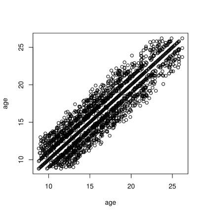
Figure 1: The design of covariance function from spinal bone mineral density data.

Specifically, we divide the covariance function into two components, the variance function and the correlation function. The former can be estimated via classic kernel smoothing, while the latter is modeled parametrically with a potentially diverging number of parameters. The principle behind this idea is to nonparametrically estimate the unknown components for which sufficient information is available while parameterizing the component with missing pieces. Since the correlation structure is usually much more structured than the covariance surface and it is possible to estimate the correlation structure nonparametrically within the diagonal band, a parametric correlation model can be selected from candidate models in existing literature and this usually works quite well to fit the unknown correlation structure.

Compared to the aforementioned works, our proposal enjoys at least two advantages. First, it can be applied to all types of designs, either sparsely/densely or regularly/irregularly observed snippets. Second, our approach is simple thanks to the parametric structure of the correlation structure, and yet powerful due to the potential to accommodate growing dimension of parameters and nonparametric variance component. We stress that, our semi-parametric and divide-and-conquer strategy is fundamentally different from the penalized basis expansion approach that is adopted in the recent paper by Lin et al. (2019) where the covariance function is represented by an analytic basis and the basis coefficients are estimated via penalized least squares. Numerical comparison of these two methods is provided in Section 5.

This divide-and-conquer approach has been explored in Fan et al. (2007) and Fan and Wu (2008) to model the covariance structure of time-varying random noise in a varying-coefficient partially linear model. We demonstrate here that a similar strategy can overcome the challenge of the missing data issue in functional snippets and further allow the dimension of the correlation function to grow to infinity. In addition, we take into account the measurement error in the observed data, which is an important component in functional data analysis but is of less interest in a partially linear model and thus not considered in Fan et al. (2007) and Fan and Wu (2008). The presence of measurement errors complicates the estimation of the variance function, as they are entangled together along the diagonal direction of the covariance surface. Consequently, the estimation procedure for the variance function in Fan et al. (2007) and Fan and Wu (2008) does not apply. While it is possible to estimate the error variance using the approach in Yao et al. (2005) and Liu and Müller (2009), these methods require a pilot estimate of the covariance function in the diagonal area, which involves two-dimensional smoothing, and thus are not efficient. A key contribution of this paper is a new estimator for the error variance in Section 3 that is simple and easy to compute. It improves upon the estimators in Yao et al. (2005) and Liu and Müller (2009), as demonstrated through theoretical analysis and numerical studies; see Section 4 and 5 for details.

2 Mean and Covariance Function Estimation

Let $X$ be a second-order random process defined on an interval $\mathcal{T}\subset\mathbb{R}$ with mean function $\mu(t)=\mathbb{E}X(t),$ and covariance function $\mathcal{C}(s,t)=\mathrm{cov}(X(s),X(t))$. Without loss of generality, we assume $\mathcal{T}=[0,1]$ in the sequel.

Suppose $\{X_{1},\ldots,X_{n}\}$ is an independent random sample of $X$, where $n$ is the sample size. In practice, functional data are rarely fully observed. Instead, they are often noisily recorded at some discrete points on $\mathcal{T}$. To accommodate this practice, we assume that each $X_{i}$ is only measured at $m_{i}$ points $T_{i1},\ldots,T_{im_{i}}$, and the observed data are $Y_{ij}=X_{i}(T_{ij})+\varepsilon_{ij}$ for $j=1,\ldots,m_{i}$, where $\varepsilon_{ij}$ represents the homoscedastic random noise such that $\mathbb{E}\varepsilon_{ij}=0$ and $\mathbb{E}\varepsilon_{ij}^{2}=\sigma_{0}^{2}$. This homoscedasticity assumption can be relaxed to accommodate heteroscedastic noise; see Section 3 for details. To further elaborate the functional snippets characterized by (S), we assume that the $i$th subject is only available to be studied between time $O_{i}-\delta/2$ and $O_{i}+\delta/2$, where the variable $O_{i}\in[\delta/2,1-\delta/2]$, called reference time in this paper, is specific to each subject and is modeled as identically and independently distributed (i.i.d.) random variables. We then assume that, $T_{i1},\ldots,T_{im_{i}}$ are i.i.d., conditional on $O_{i}$. These assumptions reflect the reality of many data collection processes when subjects enter a study at random time $O_{i}-\delta/2$ and are followed for a fixed period of time. Such a sampling plan, termed accelerated longitudinal design, has the advantage to expand the time range of interest in a short period of time as compared to a single cohort longitudinal design study.

2.1 Mean Function

Even though only functional snippets are observed rather than a full curve, smoothing approaches such as Yao et al. (2005) can be applied to estimate the mean function $\mu$, since for each $t$, there is positive probability that some design points fall into a small neighborhood of $t$. Here, we adopt a ridged version of the local linear smoothing method in Zhang and Wang (2016), as follows.

Let $K$ be a kernel function and $h_{\mu}$ a bandwidth, and define $K_{h_{\mu}}(u)=h_{\mu}^{-1}K(u/h_{\mu})$. The non-ridged local linear estimate of $\mu$ is given by $\tilde{\mu}(t)=\hat{b}_{0}$ with

$$(\hat{b}_{0},\hat{b}_{1})=\underset{(b_{0},b_{1})\in\mathbb{R}^{2}}{\arg\min}\sum_{i=1}^{n}w_{i}\sum_{j=1}^{m_{i}}K_{h_{\mu}}(T_{ij}-t)\{Y_{ij}-b_{0}-b_{1}(T_{ij}-t)\}^{2},$$

where $w_{i}\geq 0$ are weight such that $\sum_{i=1}^{n}m_{i}w_{i}=1$. For the optimal choice of weight, readers are referred to Zhang and Wang (2018). It can be shown that $\tilde{\mu}(t)=(R_{0}S_{2}-R_{1}S_{1})/(S_{0}S_{2}-S_{1}^{2})$, where

$$S_{r} =\sum_{i=1}^{n}w_{i}\sum_{j=1}^{m_{i}}K_{h_{\mu}}(T_{ij}-t)\{(T_{ij}-t)/h_{\mu}\}^{r},$$

$$R_{r} =\sum_{i=1}^{n}w_{i}\sum_{j=1}^{m_{i}}K_{h_{\mu}}(T_{ij}-t)\{(T_{ij}-t)/h_{\mu}\}^{r}Y_{ij}.$$

Although $\tilde{\mu}$ behaves well most of the time, for a finite sample, there is positive probability that $S_{0}S_{2}-S_{1}^{2}=0$, hence $\tilde{\mu}$ may become undefined. This minor issue can be addressed by ridging, a regularization technique used by Fan (1993) with details in Seifert and Gasser (1996) and Hall and Marron (1997). The basic idea is to add a small positive constant to the denominator of $\tilde{\mu}$ when $S_{0}S_{2}-S_{1}^{2}$ falls below a threshold. More specifically, the ridged version of $\tilde{\mu}(t)$ is given by

$$\hat{\mu}(t)=\frac{R_{0}S_{2}-R_{1}S_{1}}{S_{0}S_{2}-S_{1}^{2}+\Delta 1_{\{|S_{0}S_{2}-S_{1}^{2}|<\Delta\}}},$$ (2)

where $\Delta$ is a sufficiently small constant depending on $n$ and $m_{1},\ldots,m_{n}$. A convenient choice here is $\Delta=(nm)^{-2}$, where $m=n^{-1}\sum_{i=1}^{n}m_{i}$.

The tuning parameter $h_{\mu}$ could be selected via the following $\kappa$-fold cross-validation procedure. Let $\kappa$ be a positive integer, e.g., $\kappa=5$, and $\{\mathcal{P}_{1},\ldots,\mathcal{P}_{\kappa}\}$ be a roughly even random partition of the set $\{1,\ldots,n\}$. For a set $\mathcal{H}$ of candidate values for $h_{\mu}$, we choose one from it such that the following cross-validation error

$$\mathrm{CV}(h)=\sum_{k=1}^{\kappa}\sum_{i\in\mathcal{P}_{k}}\sum_{j=1}^{m_{i}}\{Y_{ij}-\hat{\mu}_{h,-k}(T_{ij})\}^{2}$$ (3)

is minimized, where $\hat{\mu}_{h,-k}$ is the estimator in (2) with $h_{\mu}=h$ and subjects in $\mathcal{P}_{k}$ excluded.

2.2 Covariance Function

Estimation of the covariance function $\mathcal{C}(s,t)$ for functional snippets is considerably more challenging. As we have pointed out in Section 1, local information in the far off-diagonal region, $|s-t|>\delta$, is completely missing. To tackle this challenge, we first observe that the covariance function can be decomposed into two parts, a variance function and a correlation structure, i.e., $\mathcal{C}(s,t)=\sigma_{X}(s)\sigma_{X}(t)\rho(s,t)$, where $\sigma_{X}^{2}(\cdot)$ is the variance function of $X$, or more precisely, $\sigma_{X}^{2}(t)=\mathbb{E}\{X(t)-\mu(t)\}^{2}$, and $\rho(\cdot,\cdot)$ is the correlation function. Like the mean function $\mu$, the variance function can be well estimated via local linear smoothing even in the case of functional snippets. The real difficulty stems from the estimation of the correlation structure, which we propose to model parametrically. At first glance, a parametric model might be restrictive. However, with a nonparametric variance component and a large number of parameters, the model will often still be sufficiently flexible to capture the covariance structure of the data. Indeed, in our simulation studies that are presented in Section 5, we demonstrate that even with a single parameter, the proposed model often yields good performance when sample size is limited. As an additional flexibility, our parametric model does not require the low-rank assumption and hence is able to model truly infinitely-dimensional functional data. This trade of the low-rank assumption with the proposed parametric assumption seems worthwhile, especially because we allow the dimension of the parameters to increase with the sample size. The increasing dimension of the parameter essentially puts the methodology in the nonparametric paradigm.

To estimate $\sigma_{X}^{2}(\cdot)$, we first note that the PACE method in Yao et al. (2005) can still be used to estimate $\mathcal{C}(s,t)$ on the band $\mathcal{T}_{\delta}^{2}=\{(s,t)\in\mathcal{T}\times\mathcal{T}:\,|s-t|<\delta\}$ that includes the diagonal, although not on the full domain $\mathcal{T}\times\mathcal{T}$. Since $\sigma_{X}^{2}(t)=\mathcal{C}(t,t)$, the PACE estimate $\tilde{\mathcal{C}}$ for $\mathcal{C}$ on the diagonal gives rise to an estimate of $\sigma_{X}^{2}(t)$. However, this method requires two-dimensional smoothing, which is cumbersome and computationally less efficient. In addition, it has the convergence rate of a two-dimensional smoother, which is suboptimal for a target $\sigma_{X}^{2}(t)$ that is a one-dimensional function. Here we propose a simpler approach that only requires one-dimensional smoothing, based on the observation that the quantity $\varsigma^{2}(t)\equiv\mathbb{E}\{Y(t)-\mu(t)\}^{2}=\sigma_{X}^{2}(t)+\sigma_{0}^{2}$ can be estimated by local linear smoothing on the observations $\{Y_{ij}-\hat{\mu}(T_{ij})\}^{2}$. More specifically, the non-ridged local linear estimate of $\varsigma^{2}(t)$, denoted by $\tilde{\varsigma}^{2}(t)$, is $\hat{b}_{0}$ with

$$(\hat{b}_{0},\hat{b}_{1})=\underset{(b_{0},b_{1})\in\mathbb{R}^{2}}{\arg\min}\sum_{i=1}^{n}w_{i}\sum_{j=1}^{m_{i}}K_{h_{\sigma}}(T_{ij}-t)[\{Y_{ij}-\hat{\mu}(T_{ij})\}^{2}-b_{0}-b_{1}(T_{ij}-t)]^{2},$$

where $h_{\sigma}$ is the bandwidth to be selected by a cross-validation procedure similar to (3). As with the ridged estimate of the mean function in (2), to circumvent the positive probability of being undefined for $\tilde{\varsigma}^{2}$, we adopt the ridged version of $\tilde{\varsigma}^{2}$ as the estimate for $\varsigma^{2}$, denoted by $\hat{\varsigma}^{2}$. Then our estimate of $\sigma_{X}^{2}(t)$ is $\hat{\sigma}_{X}^{2}(t)=\hat{\varsigma}^{2}(t)-\hat{\sigma}^{2}_{0}$, where $\hat{\sigma}^{2}_{0}$ is a new estimate of $\sigma_{0}^{2}$, to be defined in the next section, that has a convergence rate of a one-dimensional smoother. Because $\hat{\varsigma}^{2}(t)$ also has a one-dimensional convergence, the resulting estimate of $\hat{\sigma}_{X}^{2}(t)$ has a one-dimensional convergence rate.

For the correlation function $\rho$, we assume that $\rho$ is indexed by a $d_{n}$-dimensional vector of parameters, denoted by $\theta\in\mathbb{R}^{d_{n}}$. Here, the dimension of parameters is allowed to grow with the sample size at a certain rate; see Section 4 for details. Some popular parametric families for correlation function are listed below.

1. Power exponential:

   $$\rho_{\theta}(s,t)=\exp\left\{-\frac{|s-t|^{\theta_{1}}}{\theta_{2}^{\theta_{1}}}\right\},\quad 0<\theta_{1}\leq 2,\>\theta_{2}>0.$$

2. Rational quadratic (Cauchy):

   $$\rho_{\theta}(s,t)=\left\{1+\frac{|s-t|^{2}}{\theta_{2}^{2}}\right\}^{-\theta_{1}},\quad\theta_{1},\theta_{2}>0.$$

3. Matérn:

   $$\rho_{\theta}(s,t)=\frac{1}{\Gamma(\theta_{1})2^{\theta_{1}-1}}\left(\sqrt{2\theta_{1}}\frac{|s-t|}{\theta_{2}}\right)^{\theta_{1}}B_{\theta_{1}}\left(\sqrt{2\theta_{1}}\frac{|s-t|}{\theta_{2}}\right),\quad\theta_{1},\theta_{2}>0,$$ (4)

   with $B_{\theta}(\cdot)$ being the modified Bessel function of the second kind of order $\theta$.

Note that if $\rho_{1},\ldots,\rho_{p}$ are correlation functions, then $\sum_{k=1}^{p}v_{k}\rho_{k}$ is also a correlation function if $\sum_{k=1}^{p}v_{k}=1$ and $v_{k}\geq 0$ for all $k$. Therefore, a fairly flexible class of correlation functions can be constructed from several relatively simple classes by this convex combination. We point out here that, even when one adopts a stationary correlation function, the resulting covariance can be non-stationary due to a nonparametric and hence often non-stationary variance component.

Given the estimate $\hat{\sigma}^{2}_{X}(t)$, the parameter $\theta$ can be effectively estimated using the following least squares criterion, i.e., $\hat{\theta}=\underset{\theta}{\arg\min}\,\,\hat{Q}_{n}(\theta)$ with

$$\hat{Q}_{n}(\theta)=\sum_{i=1}^{n}\frac{1}{m_{i}(m_{i}-1)}\sum_{1\leq j\neq l\leq m_{i}}\{\hat{\sigma}_{X}(T_{ij})\hat{\sigma}_{X}(T_{il})\rho_{\theta}(T_{ij},T_{il})-C_{ijl}\}^{2},$$

where $C_{ijl}=\{Y_{ij}-\hat{\mu}(T_{ij})\}\{Y_{il}-\hat{\mu}(T_{il})\}$ is the raw covariance of subject $i$ at two different measurement times, $T_{ij}$ and $T_{il}$.

3 Estimation of Noise Variance

The estimation of $\sigma_{0}^{2}$ received relatively little attention in the literature. For sparse functional data, the PACE estimator $2|\mathcal{T}|^{-1}\int_{\mathcal{T}}\{\hat{\varsigma}(t)-\hat{\mathcal{C}}(t,t)\mathrm{d}t\}$ proposed in Yao et al. (2005) is a popular option. However, the PACE estimator can be negative in some cases. Liu and Müller (2009) refined this PACE estimator by first fitting the observed data using the PACE estimator and then estimating $\sigma_{0}^{2}$ by cross-validated residual sum of squares; see appendix A.1 of Liu and Müller (2009) for details. These methods require an estimate of the covariance function, which we do not have here before we obtain an estimate of $\sigma_{0}^{2}$. Moreover, the estimate $\hat{\mathcal{C}}(t,t)$ in both methods is obtained by two-dimensional local linear smoothing as detailed in Yao et al. (2005), which is computationally costly and leads to a slower (two-dimensional) convergence rate of these estimators. To resolve this conundrum, we propose the following new estimator that does not require estimation of the covariance function or any other parameters such as the mean function.

For a bandwidth $h_{0}>0$, define the quantities

$$A_{0} =\mathbb{E}[\{\mathcal{C}(T_{1},T_{1})+\mu(T_{1})\mu(T_{1})+\sigma_{0}^{2}\}1_{|T_{1}-T_{2}|<h_{0}}],$$

$$A_{1} =\mathbb{E}[\{\mathcal{C}(T_{1},T_{1})+\mu(T_{1})\mu(T_{1})\}1_{|T_{1}-T_{2}|<h_{0}}],$$

and

$$B=\mathbb{E}1_{|T_{1}-T_{2}|<h_{0}},$$

where $T_{1}$ and $T_{2}$ denote two design points from the same generic subject. From the above definition, we immediately see that $A_{0}=A_{1}+B\sigma_{0}^{2}$. Also, these quantities seem easy to estimate. For example, $A_{0}$ and $B$ can be straightforwardly estimated respectively by

$$\hat{A}_{0}=\frac{1}{n}\sum_{i=1}^{n}\frac{1}{m_{i}(m_{i}-1)}\sum_{j\neq l}Y_{ij}^{2}1_{|T_{ij}-T_{il}|<h_{0}}$$ (5)

and

$$\hat{B}=\frac{1}{n}\sum_{i=1}^{n}\frac{1}{m_{i}(m_{i}-1)}\sum_{j\neq l}1_{|T_{ij}-T_{il}|<h_{0}}.$$ (6)

This motivates us to estimate $\sigma_{0}^{2}$ via estimation of $A_{0}$, $A_{1}$ and $B$.

It remains to estimate $A_{1}$, which cannot be estimated using information along the diagonal only, due to the presence of random noise. Instead, we shall explore the smoothness of the covariance function and observe that if $T_{1}$ is close to $T_{2}$, say $|T_{1}-T_{2}|<h_{0}$, then $\mathcal{C}(T_{1},T_{1})\approx\mathcal{C}(T_{1},T_{2})$ and

$$A_{1}\approx A_{2}=\mathbb{E}[\{\mathcal{C}(T_{1},T_{2})+\mu(T_{1})\mu(T_{2})\}1_{|T_{1}-T_{2}|<h_{0}}].$$

Indeed, we show in Lemma 5 that $A_{1}=A_{2}+O(h_{0}^{3})$. Therefore, it is sensible to use $A_{2}$ as a surrogate of $A_{1}$. The former can be effectively estimated by

$$\hat{A}_{2}=\frac{1}{n}\sum_{i=1}^{n}\frac{1}{m_{i}(m_{i}-1)}\sum_{j\neq l}Y_{ij}Y_{il}1_{|T_{ij}-T_{il}|<h_{0}},$$ (7)

and we set $\hat{A}_{1}=\hat{A}_{2}$. Finally, the estimate of $\sigma_{0}^{2}$ is given by

$$\hat{\sigma}_{0}^{2}=(\hat{A}_{0}-\hat{A}_{1})/\hat{B}.$$ (8)

To choose $h_{0}$, motivated by the convergence rate stated in Theorem 1 of the next section, we suggest the following empirical rule, $h_{0}=0.29\hat{\delta}\|\hat{\varsigma}\|_{2}(nm^{2})^{-1/5}$, for sparse functional snippets, where $\hat{\delta}=\max_{1\leq i\leq n}\max_{1\leq j,l\leq m_{i}}|T_{ij}-T_{il}|$ acts as an estimate for $\delta$, $m=n^{-1}\sum_{i=1}^{n}m_{i}$ represents the average number of measurements per curve, $\hat{\varsigma}^{2}(t)$ is the estimate of $\varsigma^{2}(t)=\sigma_{X}^{2}(t)+\sigma_{0}^{2}$ defined in Section 2, and $\|\hat{\varsigma}\|_{2}^{2}=\int\hat{\varsigma}^{2}(t)\mathrm{d}t$ represents the overall variability of the data. The coefficient $0.29$ is determined by a method described in the appendix. If this rule yields a value of $h_{0}$ that makes the neighborhood $\mathcal{N}(h_{0})=\{(T_{ij},T_{il}):|T_{ij}-T_{il}|<h_{0},i=1,\ldots,n,1\leq j\neq l\leq m_{i}\}$ empty or contain too few points, then we recommend to choose the minimal value of $h_{0}$ such that $\mathcal{N}(h_{0})$ contains at least $10^{-1}\sum_{i=1}^{n}m_{i}(m_{i}-1)$ points. In this way, we ensure that a substantial fraction of the observed data are used for estimation of the variance $\sigma_{0}^{2}$. This rule is found to be very effective in practice; see Section 5 for its numerical performance.

Compared to Yao et al. (2005) and Liu and Müller (2009), the proposed estimate (8) is simple and easy to compute. Indeed, it can be computed much faster since it does not require the costly computation of $\hat{\mathcal{C}}$. More importantly, the ingredients $\hat{A}_{0}$, $\hat{A}_{1}=\hat{A}_{2}$ and $\hat{B}$ for our estimator are obtained by one-dimensional smoothing, with the term $1_{|T_{ij}-T_{il}|<h_{0}}$ in (5)–(7) acting as a local constant smoother. Consequently, as we show in Section 4, our estimator enjoys an asymptotic convergence rate that is faster than the one from a two-dimensional local linear smoother. In addition, the proposed estimate is always nonnegative, in contrast to the one in Yao et al. (2005). This is seen by the following derivation:

$$\hat{A}_{1} =\frac{1}{n}\sum_{i=1}^{n}\frac{1}{m_{i}(m_{i}-1)}\sum_{j\neq l}Y_{ij}Y_{il}1_{|T_{ij}-T_{il}|<h_{0}}\leq\frac{1}{n}\sum_{i=1}^{n}\frac{1}{m_{i}(m_{i}-1)}\sum_{j\neq l}\frac{Y_{ij}^{2}+Y_{il}^{2}}{2}1_{|T_{ij}-T_{il}|<h_{0}}$$

$$=\frac{1}{n}\sum_{i=1}^{n}\frac{1}{m_{i}(m_{i}-1)}\sum_{j\neq l}Y_{ij}^{2}1_{|T_{ij}-T_{il}|<h_{0}}=\hat{A}_{0}.$$ (9)

Remark: The above discussion assumes that the noise is homoscedastic, i.e., its variance is identical for all $t$. As an extension, it is possible to modify the above procedure to account for heteroscedastic noise, as follows. With intuition and rationale similar to the homoscedastic case, we define

$$\hat{A}_{0}(t) =\frac{1}{n}\sum_{i=1}^{n}\frac{1}{m_{i}(m_{i}-1)}\sum_{j\neq l}Y_{ij}^{2}1_{|T_{ij}-t|<h_{0}}1_{|T_{il}-t|<h_{0}},$$

$$\hat{A}_{1}(t) =\frac{1}{n}\sum_{i=1}^{n}\frac{1}{m_{i}(m_{i}-1)}\sum_{j\neq l}Y_{ij}Y_{il}1_{|T_{ij}-t|<h_{0}}1_{|T_{il}-t|<h_{0}},$$

$$\hat{B}(t) =\frac{1}{n}\sum_{i=1}^{n}\frac{1}{m_{i}(m_{i}-1)}\sum_{j\neq l}1_{|T_{ij}-t|<h_{0}}1_{|T_{il}-t|<h_{0}},$$

and let

$$\hat{\sigma}_{0}^{2}(t)=\{\hat{A}_{0}(t)-\hat{A}_{1}(t)\}/\hat{B}(t)$$

be the estimate of $\sigma_{0}^{2}(t)$ which is the variance of the noise at $t\in\mathcal{T}$. Like the derivation in (9), one can also show that this estimator is nonnegative.

4 Theoretical Properties

For clarity of exposition, we assume throughout this section that all the $m_{i}$ have the same rate $m$, i.e., $m_{i}=m$, where the sampling rate $m$ may tend to infinity. We emphasize that parallel asymptotic results can be derived without this assumption by replacing $m$ with $\frac{1}{n}\sum_{i=1}^{n}m_{i}$. Note that the theory to be presented below applies to both the case that $m$ is bounded by a constant, i.e., $m\leq m_{0}$ for some $m_{0}<\infty$, and the case that $m$ diverges to $\infty$ as $n\rightarrow\infty$.

We assume that the reference time $O_{i}$ is identically and independently distributed (i.i.d.) sampled from a density $f_{O}$, and $T_{i1},\ldots,T_{im_{i}}$ are i.i.d., conditional on $O_{i}$. The i.i.d. assumptions can be relaxed to accommodate heterogeneous distributions and weak dependence, at the cost of much more complicated analysis and heavy technicalities. As such relaxation does not provide further insight into our problem, we decide not to pursue it in the paper. The following conditions about $O_{i}$ and other quantities are needed for our theoretical development.

1. The density $f_{O}$ of each $O_{i}$ satisfies $f_{O}(u)>0$ for all $u\in[\delta/2,1-\delta/2]$, and the conditional density $f_{T|O}$ of $T_{ij}$ given $O_{i}$ satisfies $f_{T|O}(t|u)=f_{0}(t-u+\delta/2)>0$ for a fixed function $f_{0}$ and for all $u\in[\delta/2,1-\delta/2]$ and $t\in[u-\delta/2,u+\delta/2]$. Also, the derivative $\frac{\mathrm{d}}{\mathrm{d}t}f_{0}(t)$ is Lipschitz continuous on $[0,\delta]$.

2. The second derivatives of $\mu$ and $\mathcal{C}$ are continuous and hence bounded on $\mathcal{T}$ and $\mathcal{T}\times\mathcal{T}$, respectively.

3. $\mathbb{E}\|X\|^{4}<\infty$ and $\mathbb{E}\varepsilon^{4}<\infty$.

In the above, the condition (A1) characterizes the design points for functional snippets and can be relaxed, while the regularity conditions (A2) and (A3) are common in the literature, e.g., in Zhang and Wang (2016). According to Scheuerer (2010), (A2) also implies that the sample paths of $X$ are continuously differentiable and hence Lipschitz continuous almost surely. Let $L_{X}$ be the best Lipschitz constant of $X$, i.e., $L_{X}=\inf\{C\in\mathbb{R}:\,|X(s)-X(t)|\leq C|s-t|\text{ for all }s,t\in\mathcal{T}\}$. We will see shortly that a moment condition on $L_{X}$ allows us to derive a rather sharp bound for the convergence rate of $\hat{\sigma}_{0}^{2}$. For the bandwidth $h_{0}$, we require the following condition:

1. $h_{0}\rightarrow 0$ and $nm^{2}h_{0}\rightarrow\infty$.

The following result gives the asymptotic rate of the estimator $\hat{\sigma}_{0}^{2}$. The proof is straightforward once we have Lemma 5, which is given in the appendix.

Theorem 1.

Assume the conditions (A1)–(A3) and (H1) hold.

1. $(\hat{\sigma}_{0}^{2}-\sigma_{0}^{2})^{2}=O_{P}(h_{0}^{4}+n^{-1}+n^{-1}m^{-2}h_{0}^{-1})$. With the optimal choice $h_{0}\asymp(nm^{2})^{-1/5}$, $(\hat{\sigma}_{0}^{2}-\sigma_{0}^{2})^{2}=O_{P}(n^{-4/5}m^{-8/5}+n^{-1})$.

2. If in addition $\mathbb{E}L_{X}^{4}<\infty$, then $(\hat{\sigma}_{0}^{2}-\sigma_{0}^{2})^{2}=O_{P}(h_{0}^{4}+n^{-1}m^{-1}+n^{-1}m^{-2}h_{0}^{-1})$. With the optimal choice $h_{0}\asymp(nm^{2})^{-1/5}$, $(\hat{\sigma}_{0}^{2}-\sigma_{0}^{2})^{2}=O_{P}(n^{-4/5}m^{-8/5}+n^{-1}m^{-1})$.

If we define $\hat{\sigma}_{0}^{2}=(\hat{A}_{0}-\hat{A}_{1})/(\hat{B}+\Delta)$ with $\Delta=(nm)^{-2}h_{0}$, the ridged version of (8), then in the above theorem, $(\hat{\sigma}_{0}^{2}-\sigma_{0}^{2})^{2}$ can be replaced with $\mathbb{E}(\hat{\sigma}_{0}^{2}-\sigma_{0}^{2})^{2}$ and $O_{P}(\cdot)$ can be replaced with $O(\cdot)$, respectively. For comparison, under conditions stronger than (A1)–(A3), the rate derived in Yao et al. (2005) for the PACE estimator is at best $(\hat{\sigma}_{0}^{2}-\sigma_{0}^{2})^{2}=O_{P}(n^{-1/2})$. This rate was improved by Paul and Peng (2011) to $\mathbb{E}(\hat{\sigma}_{0}^{2}-\sigma_{0}^{2})^{2}=O(n^{-1}+n^{-4/5}m^{-4/5}+n^{-2/3}m^{-4/3})$. Our estimator clearly enjoys a faster convergence rate, in addition to its computational efficiency. The rate in part (b) of Theorem 1 has little room for improvement, since when $n$ is finite but $m\rightarrow\infty$, the rate is optimal, i.e., $\mathbb{E}(\hat{\sigma}_{0}^{2}-\sigma_{0}^{2})^{2}=O(m^{-1})$. When $m$ is finite but $n\rightarrow\infty$ in the sparse design, we obtain $\mathbb{E}(\hat{\sigma}_{0}^{2}-\sigma_{0}^{2})^{2}=O(n^{-4/5})$, in contrast to the rate $O_{P}(n^{-2/3})$ for the PACE estimator according to Paul and Peng (2011).

To study the properties of $\hat{\mu}(t)$ and $\hat{\sigma}^{2}(t)$, we shall assume

1. the kernel $K$ is a symmetric and Lipschitz continuous density function supported on $[-1,1]$.

Also, the bandwidth $h_{\mu}$ and $h_{\sigma}$ are assumed to meet the following conditions.

1. $h_{\mu}\rightarrow 0$ and $nmh_{\mu}\rightarrow\infty$.

2. $h_{\sigma}\rightarrow 0$ and $nmh_{\sigma}\rightarrow\infty$.

The choice of these bandwidths depends on the interplay of the sampling rate $m$ and sample size $n$. The optimal choice is given in the following condition.

1. If $m\lesssim n^{1/4}$, then $h_{\mu}\asymp h_{\sigma}\asymp(nm)^{-1/5}$, where the notation $a_{n}\lesssim b_{n}$ means $\lim_{n\rightarrow\infty}a_{n}/b_{n}<\infty$. Otherwise, $\max\{h_{\mu},h_{\sigma}\}\asymp n^{-1/4}$. Also, $h_{0}\asymp(nm^{2})^{-1/5}$.

The asymptotic convergence rates for $\hat{\mu}$ and $\hat{\sigma}_{X}^{2}$ are given in the following theorem, whose proof can be obtained by adapting the proof of Proposition 1 in Lin and Yao (2020+) and hence is omitted. It shows that both $\hat{\mu}$ and $\hat{\sigma}_{X}^{2}$ have the same rate, which is hardly surprising since they are both obtained by a one-dimensional local linear smoothing technique. Note that our results generalize those in Fan et al. (2007) and Fan and Wu (2008) by taking the measurement errors and the order of the sampling rate $m$ into account in the theoretical analysis. In addition, our $\mathcal{L}^{2}$ convergence rates of these estimators complement the asymptotic normality results in Fan et al. (2007) and Fan and Wu (2008).

Theorem 2.

Suppose the conditions (A1)–(A3) hold.

1. With additional conditions (B1) and (H2), $\mathbb{E}\|\hat{\mu}-\mu\|^{2}=O(h_{\mu}^{4}+n^{-1}+n^{-1}m^{-1}h_{\mu}^{-1})$. With the choice of bandwidth $h_{\mu}$ in (H4), $\mathbb{E}\|\hat{\mu}-\mu\|^{2}=O\left((nm)^{-4/5}+n^{-1}\right)$.

2. With additional conditions (B1) and (H1)–(H3), $\mathbb{E}\|\hat{\sigma}_{X}^{2}-\sigma_{X}^{2}\|^{2}=O(h_{\sigma}^{4}+h_{\mu}^{4}+h_{0}^{4}+n^{-1}+n^{-1}m^{-1}h_{\sigma}^{-1}+n^{-1}m^{-1}h_{\mu}^{-1}+n^{-1}m^{-2}h_{0}^{-1})$. With the choice of bandwidth in (H4), $\mathbb{E}\|\hat{\sigma}_{X}^{2}-\sigma_{X}^{2}\|^{2}=O\left((nm)^{-4/5}+n^{-1}\right)$.

To derive the asymptotic properties of $\hat{\mathcal{C}}(s,t)=\hat{\sigma}_{X}(s)\rho_{\hat{\theta}}(s,t)\hat{\sigma}_{X}(t)$, we need the convergence rate of $\hat{\theta}$. Define

$$Q(\theta) =\mathbb{E}\{\sigma_{X}(T_{11})\sigma_{X}(T_{12})\rho_{\theta}(T_{11},T_{12})-[Y_{11}-\mu(T_{11})][Y_{12}-\mu(T_{12})]\}^{2},$$

and assume the following conditions.

1. $\rho_{\theta}(s,t)$ is twice continuously differentiable with respect to $s$ and $t$. Furthermore, the first three derivatives of $\rho_{\theta}(s,t)$ with respect to $\theta$ are uniformly bounded for all $\theta,s,t,d_{n}$.

2. $\lambda_{\min}\left(\frac{\partial^{2}Q}{\partial\theta^{2}}\mid_{\theta=\theta_{0}}\right)>c_{0}d_{n}^{-\tau}$ for some $c_{0}>0$ and $\tau\geq 0$, where $\theta_{0}$ denotes the true value of $\theta$, and $\lambda_{\min}(\cdot)$ denotes the smallest eigenvalue of a matrix.

3. $\mathbb{E}\sup_{t}\|X(t)\|^{4+\epsilon_{0}}<\infty$ for some $\epsilon_{0}>0$ and $\mathbb{E}\varepsilon^{4}<\infty$.

Note that in the condition (B3), we allow the smallest eigenvalue of the Hessian $\frac{\partial^{2}Q}{\partial\theta^{2}}$ to decay with $d_{n}$. This, departing from the assumption in Fan and Wu (2008) of fixed dimension on the parameter $\theta$, enables us to incorporate the case that $\rho_{\theta}$ is constructed from the aforementioned convex combination of a diverging number of correlation functions, e.g., $\rho_{\theta}(s,t)=d^{-1}_{n}\sum_{j=1}^{d_{n}}\rho_{\theta_{j}}(s,t)$, where $\tau=1$ if all components $\rho_{\theta_{j}}$ satisfy (B2) uniformly. The condition (B4), although it is slightly stronger than (A3), is often required in functional data analysis, e.g., in Li and Hsing (2010) and Zhang and Wang (2016) for the derivation of uniform convergence rates for $\hat{\mu}$. Such uniform rates are required to bound $\partial\hat{Q}_{n}/\partial\theta$ sharply in our development, which is critical to establish the following rate for $\hat{\theta}$.

Proposition 3.

Suppose the conditions (A1)–(A2) and (B1)–(B4) hold. If $d_{n}=o(n^{1/(4+4\tau)})$, then with the choice of bandwidth in (H4), $\|\hat{\theta}-\theta_{0}\|^{2}=O_{P}(d_{n}^{2\tau+1}/n)$.

The above result suggests that the estimation quality of $\hat{\theta}$ depends on the dimension of parameters, sample size and singularity of the Hessian matrix at $\theta=\theta_{0}$, measured by the constant $\tau$ in condition (B3). In practice, a few parameters are often sufficient for an adequate fit. In such cases, the dimension $d_{n}$ might not grow with sample size, i.e., $d_{n}=O(1)$, and we obtain a parametric rate for $\hat{\theta}$. Now we are ready to state our main theorem that establishes the convergence rate for $\hat{\mathcal{C}}$ in the Hilbert-Schmidt norm $\|\cdot\|_{HS}$, which follows immediately from the above results.

Theorem 4.

Under the same conditions of Proposition 3, we have $\|\hat{\mathcal{C}}-\mathcal{C}\|_{HS}^{2}=O_{P}(h_{\sigma}^{4}+h_{\mu}^{4}+h_{0}^{4}+n^{-1}+n^{-1}m^{-1}h_{\sigma}^{-1}+n^{-1}m^{-1}h_{\mu}^{-1}+n^{-1}m^{-2}h_{0}^{-1}+d_{n}^{2\tau+1}n^{-1}).$ With the choice of bandwidth in (H4), $\|\hat{\mathcal{C}}-\mathcal{C}\|_{HS}^{2}=O_{P}\left((nm)^{-4/5}+d_{n}^{2\tau+1}n^{-1}\right)$.

In practice, a fully nonparametric approach like local regression to estimating the correlation structure is inefficient, in particular when data are snippets. On the other hand, a parametric method with a fixed number of parameters might be restrictive when the sample size is large. One way to overcome such a dilemma is to allow the family of parametric models to grow with the sample size. As a working assumption, one might consider that the correlation function $\rho$ falls into $\mathcal{F}_{n}$, a $d_{n}$-dimensional family of models for correlation functions, when the sample size is $n$. Here, the dimension typically grows with the sample size. For example, one might consider a $d_{n}$-Fourier basis family:

$$\kappa_{\theta}(s,t)=\frac{1}{\psi(s)\psi(t)}\sum_{j=1}^{d_{n}}\theta_{j}\phi_{j}(s)\phi_{j}(t),\quad\theta_{1},\ldots,\theta_{d_{n}}\geq 0\text{ and }\sum_{j=1}^{d_{n}}\theta_{j}=1,$$ (10)

where $\psi(t)=\left(\sum_{j=1}^{d_{n}}\theta_{j}\phi_{j}^{2}(t)\right)^{1/2}$ and $\phi_{1},\ldots$ are fixed orthonormal Fourier basis functions defined on $\mathcal{T}$. The theoretical result in Theorem 4 applies to this setting by explicitly accounting for the impact of the dimension $d_{n}$ on the convergence rate.

5 Simulation Studies

To evaluate the numerical performance of the proposed estimators, we generated $X(\cdot)$ from a Gaussian process. Three different covariance functions were considered, namely,

• $\mathcal{C}(s,t)=\sigma_{X}(s)\rho_{\theta}(s,t)\sigma_{X}(t)$ with the variance function $\sigma^{2}_{X}(t)=\sqrt{t}e^{-(t-0.1)^{2}/10}+1$ and the Matérn correlation function $\rho_{\theta=(0.5,1)}$,

• $\mathcal{C}(s,t)=\sum_{k=1}^{50}2k^{-\lambda}\phi_{k}(s)\phi_{k}(t)$ with $\lambda=2$ and Fourier basis functions $\phi_{k}(t)=\sqrt{2}\sin(2k\pi t)$, and

• $\mathcal{C}(s,t)=\sum_{1\leq j,k\leq 5}c_{jk}\phi_{j}(s)\phi_{k}(t)$ with $c_{jk}=e^{-|j-k|}/5$.

Two different sample sizes $n=50$ and $n=200$ were considered to illustrate the behavior of the estimators under a small sample size and a relatively large sample size. We set the domain $\mathcal{T}=[0,1]$ and $\delta=0.25$.

To evaluate the impact of the mean function, we also considered two different mean functions, $\mu_{1}(t)=2t^{2}\cos(2\pi t)$ and $\mu_{2}(t)=e^{t}/2$. We found that the results are not sensitive to the mean function, and thus focus only on the case $\mu_{1}(t)$ in this section; the results for the case $\mu(t)=e^{t}/2$ are provided in Supplementary Material. In addition, to evaluate the impact of the design, we considered two design schemes. In the first scheme, that is referred to as the sparse design, each curve was sparsely sampled at 4 points on average to mimic the scenario of the data application in Section 6. In the second scheme, that is referred to as the dense design, each snippet was recorded in a dense ($m_{1}=\cdots=m_{n}=26$) and regular grid of an individual specific subinterval of length $\delta$. As the focus of the paper is on sparse snippets, we report the results for the sparse design below. The results for dense snippets are reported in Supplementary Material.

To assess the performance of the estimators for the noise variance $\sigma_{0}^{2}$, we considered different noise levels $\sigma_{0}^{2}=0,0.1,0.25,0.5$, varying from no noise to large noise. For example, when $\sigma_{0}^{2}=0.5$, the signal-to-noise ratio $\mathbb{E}\|X-\mu\|^{2}/\mathrm{Var}(\varepsilon)$ is about 2. The performance of $\hat{\sigma}_{0}^{2}$ is assessed by the root mean squared error (RMSE), defined by

$$\mathrm{RMSE}=\sqrt{\frac{1}{N}\sum_{i=1}^{N}|\hat{\sigma}_{0}^{2}-\sigma_{0}^{2}|^{2}},$$

where $N$ is the number of independent simulation replicates, which we set to 100. For the purpose of comparison, we also computed the PACE estimate of Yao et al. (2005) and the estimate proposed by Liu and Müller (2009), denoted by LM, using the fdapace R package (Chen et al., 2020) that is available in the comprehensive R archive network (CRAN). The bandwidth $h_{\mu}$ and $h_{\sigma}$, as well as those in Yao et al. (2005) and Liu and Müller (2009), were selected by five-fold cross-validation. The tuning parameter $h_{0}$ was selected by the empirical rule $h_{0}=0.29\hat{\delta}\|\hat{\varsigma}\|_{2}(nm^{2})^{-1/5}$ that is described in Section 3. The simulation results are summarized in Table 1 for the sparse design with mean function $\mu_{1}$, as well as Tables S.1–S.3 for the dense design and mean function $\mu_{2}$ in Supplementary Material, where SNPT denotes our method proposed in Section 3. We observe that in almost all cases, SNPT performs significantly better than the other two methods. The results also demonstrate the effectiveness of the proposed empirical selection rule for the tuning parameter $h_{0}$.

To evaluate the performance of the estimators for the covariance structure, we considered two levels of signal-to-noise ratio (SNR), namely, $\mathrm{SNR}=2$ and $\mathrm{SNR}=4$. The performance of estimators for the variance function and the covariance function is evaluated by the root mean integrated squared error (RMISE), defined by

$$\mathrm{RMISE}=\sqrt{\frac{1}{N}\sum_{i=1}^{N}\int_{\mathcal{T}}|\hat{\sigma}^{2}_{X}(t)-\sigma^{2}_{X}(t)|^{2}\mathrm{d}t}$$

for the variance function and

$$\mathrm{RMISE}=\sqrt{\frac{1}{N}\sum_{i=1}^{N}\int_{\mathcal{T}}\int_{\mathcal{T}}|\hat{\mathcal{C}}(s,t)-\mathcal{C}(s,t)|^{2}\mathrm{d}s\mathrm{d}t}$$

for the covariance function. We compared four methods. The first two, denoted by SNPTM and SNPTF, are our semi-parametric approach with the correlation given in (4) and (10), respectively. For the SNPTF method, the dimension $d_{n}$ of (10) is selected via five-fold cross-validation. It is noted that SNPTM and SNPTF yield the same estimates of the variance function but different estimates of the correlation structure. The third one, denoted by PFBE (penalized Fourier basis expansion), is the method proposed by Lin et al. (2019), and the last one, denoted by PACE, is the approach invented by Yao et al. (2005).

For the estimation of the variance function $\sigma_{X}^{2}(t)$, the results are summarized in Table 2 for the sparse design and mean function $\mu_{1}$, and also in Tables S.4–S.6 in Supplementary Material for the dense design and mean function $\mu_{2}$. In these tables, the results of SNPTF are not reported since they are the same as the results of SNPTM. We observe that, in all cases, SNPTM and PFBE substantially outperform PACE. For the dense design, the methods SNPTM and PFBE yield comparable results. The SNPTM method performs better than PFBE when $n=200$ in most cases, except in the setting III which favors the PFBE method. This suggests that the SNPTM method, which adopts the local linear smoothing strategy combined with our estimator for the variance of the noise, generally converges faster as the sample size grows.

For the estimation of the covariance function $\mathcal{C}$, we summarize the results in Table 3 for the sparse design and mean function $\mu_{1}$, and in Tables S.7–S.9 in Supplementary Material for the dense design and mean function $\mu_{2}$. As expected, in all cases, SNPTM, SNPTF and PFBE substantially outperform PACE, since PACE is not designed to process functional snippets. Among the estimators SNPTM, SNPTF and PFBE, in the setting I, SNPTM outperforms the others since in this case the model is correctly specified for SNPTM, in the setting II, SNPTF is the best since the model is correctly specified for SNPTF, and in the setting III, PFBE has a favorable performance. Although there is no universally best estimator, overall these three estimators have comparable performance. To select a method in practice, one can first produce a scatter plot of the raw covariance function. If the function appears to decay monotonically as the point $(s,t)$ moves away from the diagonal, then SNPT with a monotonic decaying correlation such as SNPTM is recommended. Otherwise, SNPT with a general correlation structure such as SNPTF or the PFBE approach might be adopted.

Table 1: RMSE and their standard errors for $\hat{\sigma}_{0}^{2}$ under the sparse design and $\mu_{1}$

			method
Cov	$n$	$\sigma_{0}^{2}$	SNPT	PACE	LM
I	50	0	0.012 (0.009)	0.144 (0.166)	0.129 (0.203)
		0.1	0.029 (0.038)	0.129 (0.146)	0.186 (0.197)
		0.25	0.050 (0.056)	0.147 (0.185)	0.117 (0.125)
		0.5	0.100 (0.135)	0.181 (0.195)	0.157 (0.131)
	200	0	0.009 (0.005)	0.080 (0.103)	0.073 (0.077)
		0.1	0.017 (0.019)	0.091 (0.098)	0.144 (0.150)
		0.25	0.032 (0.038)	0.086 (0.097)	0.093 (0.127)
		0.5	0.049 (0.064)	0.098 (0.118)	0.165 (0.106)
II	50	0	0.036 (0.030)	0.252 (0.245)	0.219 (0.255)
		0.1	0.047 (0.052)	0.254 (0.285)	0.237 (0.255)
		0.25	0.087 (0.133)	0.241 (0.244)	0.159 (0.151)
		0.5	0.128 (0.202)	0.238 (0.260)	0.126 (0.134)
	200	0	0.024 (0.015)	0.177 (0.172)	0.192 (0.200)
		0.1	0.027 (0.027)	0.185 (0.179)	0.176 (0.174)
		0.25	0.042 (0.050)	0.177 (0.177)	0.097 (0.097)
		0.5	0.071 (0.084)	0.174 (0.182)	0.124 (0.089)
III	50	0	0.004 (0.004)	0.099 (0.103)	0.028 (0.064)
		0.1	0.024 (0.029)	0.102 (0.106)	0.099 (0.127)
		0.25	0.049 (0.063)	0.093 (0.109)	0.077 (0.080)
		0.5	0.094 (0.130)	0.113 (0.146)	0.172 (0.128)
	200	0	0.002 (0.002)	0.065 (0.077)	0.009 (0.023)
		0.1	0.010 (0.012)	0.066 (0.067)	0.049 (0.075)
		0.25	0.027 (0.033)	0.068 (0.071)	0.069 (0.067)
		0.5	0.059 (0.071)	0.067 (0.073)	0.163 (0.091)

Table 2: RMISE and their standard errors for $\hat{\sigma}^{2}_{X}(t)$ under the sparse design and $\mu_{1}$

			method
Cov	SNR	$n$	SNPTM	PFBE	PACE
I	2	50	0.535 (0.218)	0.518 (0.211)	2.133 (1.536)
		200	0.339 (0.130)	0.330 (0.118)	1.344 (1.126)
	4	50	0.531 (0.199)	0.517 (0.229)	1.845 (1.461)
		200	0.313 (0.136)	0.334 (0.127)	1.151 (0.952)
II	2	50	0.775 (0.396)	0.743 (0.214)	2.602 (1.747)
		200	0.509 (0.163)	0.530 (0.141)	1.699 (1.045)
	4	50	0.768 (0.303)	0.734 (0.351)	2.510 (1.578)
		200	0.471 (0.162)	0.507 (0.149)	1.515 (1.056)
III	2	50	0.633 (0.201)	0.592 (0.136)	1.478 (1.052)
		200	0.376 (0.133)	0.392 (0.107)	1.178 (0.700)
	4	50	0.592 (0.208)	0.586 (0.158)	1.428 (1.166)
		200	0.350 (0.139)	0.385 (0.114)	0.923 (0.451)

Table 3: RMISE and their standard errors for $\hat{\mathcal{C}}$ under the sparse design and $\mu_{1}$

			method
Cov	SNR	$n$	SNPTM	SNPTF	PFBE	PACE
I	2	50	0.339 (0.101)	0.441 (0.158)	0.399 (0.156)	1.470 (0.808)
		200	0.235 (0.092)	0.359 (0.089)	0.295 (0.101)	1.044 (0.625)
	4	50	0.315 (0.093)	0.424 (0.135)	0.371 (0.143)	1.348 (0.809)
		200	0.225 (0.084)	0.341 (0.090)	0.254 (0.097)	0.902 (0.513)
II	2	50	0.556 (0.119)	0.521 (0.183)	0.541 (0.160)	2.061 (1.061)
		200	0.474 (0.068)	0.436 (0.132)	0.465 (0.101)	1.625 (0.632)
	4	50	0.536 (0.126)	0.472 (0.148)	0.517 (0.139)	2.014 (0.868)
		200	0.457 (0.063)	0.419 (0.133)	0.431 (0.112)	1.543 (0.604)
III	2	50	0.503 (0.090)	0.511 (0.154)	0.491 (0.130)	1.248 (0.650)
		200	0.473 (0.041)	0.439 (0.092)	0.366 (0.052)	1.136 (0.439)
	4	50	0.493 (0.075)	0.499 (0.120)	0.487 (0.122)	1.217 (0.727)
		200	0.469 (0.055)	0.423 (0.087)	0.358 (0.063)	0.997 (0.316)

6 Application

We applied the proposed method to analyze the longitudinal data that was collected and detailed in Bachrach et al. (1999). It consists of longitudinal measurements of spinal bone mineral density for 423 healthy subjects. The measurement for each individual was observed annually for up to 4 years. Among 423 subjects, we focused on $n=280$ subjects ranging in age from 8.8 to 26.2 years who completed at least 2 measurements. A plot for the design of the covariance function is given in Figure 1, while a scatter plot for the raw covariance surface is given in Figure 2. The raw covariance surface seems to decay rapidly to zero as design points move away from the diagonal. This motivated us to estimate the covariance structure with a Matérn correlation function. This method is referred to as SNPTM. In addition, we also used the more flexible $d_{n}$-Fourier basis family to see whether a better fit can be achieved, where $d_{n}=2$ was selected by Akaike information criterion (AIC). Such approach is denoted by SNPTF.

The estimated variance of the measurement error is $1.5\times 10^{-3}$ by the method proposed in Section 3, $10^{-6}$ by PACE and $7.8\times 10^{-7}$ by LM, respectively. The estimates of the covariance surface are depicted in Figure 3. We observe that, the estimates produced by SNPTM and SNPTF are similar in the diagonal region, while visibly differ in the off-diagonal region. For this dataset, the upward off-diagonal parts of the estimated covariance surface by SNPTF seem artificial, so we recommend the SNPTM estimate for this data. For the PACE estimate, due to the missing data in the off-diagonal region and insufficient observations at two ends of the diagonal region, it suffers from significant boundary effect.

The mean function estimated by SNPTM shown in the left panel of Figure 4 and found similar to its counterpart in Lin et al. (2019), suggests that the spinal bone mineral density increases rapidly from age 9 to age 16, and then slows down afterward. The mineral density has the largest variation around age 14, indicated by the variance function estimated by SNPTM and shown in the middle panel of Figure 4. As a comparison, the PACE estimate, shown in the right panel of Figure 4, suffers from the boundary effect that is passed from the PACE estimate of the covariance function, because the PACE method estimates the variance function by the diagonal of the estimated covariance function.

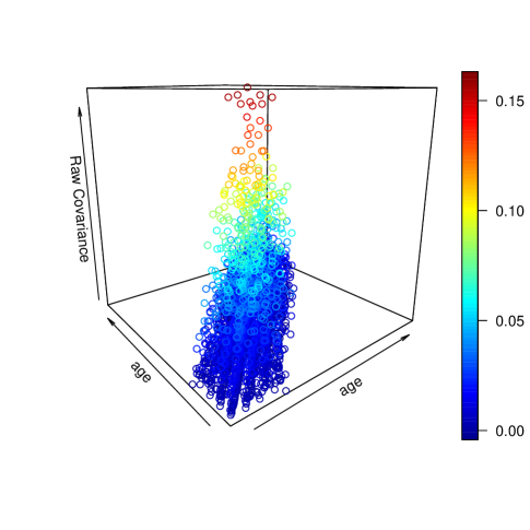
Figure 2: Scatter plot of the raw covariance function of the spinal bone mineral density data.

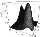
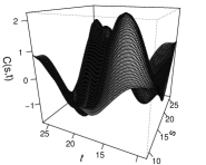
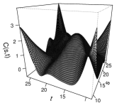
Figure 3: The estimated covariance functions by SNPTM (left), SNPTF (middle) and PACE (right). The $z$-axis is scaled by $10^{-2}$ for visualization.

Figure 4: The estimated mean function (left), the estimated variance function by SNPTM and SNPTF (middle), and the estimated variance function by PACE (right).

7 Concluding Remarks

In this paper, we consider the mean and covariance estimation for functional snippets. The estimation of the mean function is still an interpolation problem so previous approaches based on local smoothing methods still work, except that the theory needs a little adjustment to reflect the new design of functional snippets. However, the estimation of the covariance function is quite different because it is now an extrapolation problem rather an interpolation problem, so previous approaches based on local smoothing do not work anymore. We propose a hybrid approach that leverages the available information and structure of the correlation in the diagonal band to estimate the correlation function parametrically but the variance function nonparametrically. Because the dimension of the parameters can grow with the sample size, the approach is very flexible and can be made nearly nonparametric for the final covariance estimate.

An interesting feature of the algorithm is that it reverses the order of estimation for the variance components, compared to existing approaches for non-snippets functional data, by first estimating the noise variance $\sigma_{0}$, then estimating the variance function $\sigma_{X}^{2}(t)$, followed by the fitting of the correlation function. The estimation of the covariance function is performed at the very end when all other components have been estimated. The proposed approach differs substantially from traditional approaches, such as PACE (Yao et al., 2005), which estimate the covariance function first, from there the variance function is obtained as a byproduct through the diagonal elements of the covariance estimate, while the noise variance is estimated at the very end. The new procedure to estimate the noise variance is both simpler and better than the PACE estimates. Thus, even if the data are non-snippet types, one can use the new method proposed in Section 3 to estimate the noise variance.

We emphasize that, although the proposed method targets functional snippets, it is also applicable to functional fragments or functional data in which each curve consists of multiple disjoint snippets. In addition, the theory presented in Section 4 can be slightly modified to accommodate such data. In contrast, methods designed for nonsnippet functional data are generally not applicable to functional snippets, due to the reasons discussed in Section 1. In practice, one might distinguish between functional snippets and nonsnippets by the design plot like Figure 1. If the support points cover the entire region, then the data are of the nonsnippet type. Otherwise they are functional snippets. However, there might be some case that it is unclear whether the entire region is fully covered by support points, especially when data are sparsely observed. In such situation, snippet-based methods, such as the proposed one, is a safer option.

Reliable estimates of the mean and covariance functions are fundamental to the analysis of functional data. They are also the building blocks of functional regression methods and functional hypothesis test procedures. The proposed estimators for the mean and covariance of functional snippets together provide a stepping stone to future study on regression and inference that are specific to functional snippets.

Supplementary Material

The online supplementary material contains additional simulation results, as well as information for implementation of the proposed method in the R package mcfda.

Appendix

Selection of $h_{0}$

The constant $0.29$ in the empirical rule $h_{0}=0.29\hat{\delta}\|\hat{\varsigma}\|_{2}(nm^{2})^{-1/5}$ presented in Section 3 was determined by optimizing $\sum\{\hat{h}-c\hat{\delta}\|\hat{\varsigma}\|_{2}(nm^{2})^{-1/5}\}^{2}$ over $c\in\mathbb{R}$, where the summation is taken over the combinations of various parameters. Specifically, for each tuple $(n,m,\delta,\sigma_{0}^{2},\mathcal{C})$, we generated a batch of $G=100$ independent datasets of $n$ centered Gaussian snippets with the covariance function $\mathcal{C}$. Each snippet was recorded at $m$ random points from a random subinterval of length $\delta$ in $[0,1]$. For each batch of datasets, we found $\hat{h}$ to minimize $\sum_{r=1}^{G}\{\hat{\sigma}_{0,r}^{2}(\hat{h})-\sigma_{0}^{2}\}^{2}$, where $\hat{\sigma}_{0,r}^{2}(\hat{h})$ is the estimate of $\sigma_{0}^{2}$ based the $r$th dataset in the batch and by using the proposed method with the bandwidth $\hat{h}$. We also obtained the quantities $\hat{\delta}=G^{-1}\sum_{r=1}^{G}\hat{\delta}_{r}$ and $\|\hat{\varsigma}\|_{2}=G^{-1}\sum_{r=1}^{G}\|\hat{\varsigma}_{r}\|_{2}$, where $\hat{\delta}_{r}$ and $\hat{\varsigma}_{r}$ are the estimate of $\delta$ and $\varsigma$ based on the $r$th dataset in the batch, respectively. In this way, we obtain a collection $\mathscr{H}$ of vectors $(\hat{h},n,m,\hat{\delta},\|\hat{\varsigma}\|_{2})$. Finally, we found $c=0.29$ to minimize $\sum\{\hat{h}-c\hat{\delta}\|\hat{\varsigma}\|_{2}(nm^{2})^{-1/5}\}^{2}$, where the summation is taken over the collection $\mathscr{H}$.

In the above process, the covariance function $\mathcal{C}$ was taken from a collection composed by 1) covariance functions whose correlation part is the correlation function listed in Section 2 with various values of the parameters and whose variance functions are exponential functions, squared sin/cos functions and positive polynomials, 2) covariance functions $\mathcal{C}(s,t)=a\min\{s,t\}$ with various values of $a>0$, 3) covariance functions $\mathcal{C}(s,t)=\sum_{k=1}^{K}ak^{-\lambda}\phi_{k}(s)\phi_{k}(t)$ with various values of $a>0$, $\lambda>0$ and $K\geq 1$, where the functions $\phi_{k}$ are the Fourier basis functions described in Section 5, and 4) covariance functions $\mathcal{C}(s,t)=\sum_{1\leq j,k\leq K}ae^{-b|j-k|}$ with various choices of $a>0$, $b>0$ and $K\geq 1$.

Technical Lemmas

Lemma 5.

1. Under conditions (A1)–(A2), one has $A_{2}=A_{1}+O(h_{0}^{3})$.

2. With condition (A1), $\mathbb{E}(\hat{B}-B)^{2}=O(n^{-1}m^{-2}h_{0}+n^{-1}m^{-1}h_{0}^{2})$.

3. Under conditions (A1)–(A3), $\mathbb{E}\{(\hat{A}_{0}-\hat{A}_{1})-(A_{0}-A_{1})\}^{2}=O(h_{0}^{6}+n^{-1}m^{-2}h_{0}+n^{-1}h_{0}^{2})$. If $\mathbb{E}L_{X}^{4}<\infty$ is also assumed, then $\mathbb{E}\{(\hat{A}_{0}-\hat{A}_{1})-(A_{0}-A_{1})\}^{2}=O(h_{0}^{6}+n^{-1}m^{-2}h_{0}+n^{-1}m^{-1}h_{0}^{2})$.

Proof.

To show $A_{2}=A_{1}+O(h_{0}^{3})$ in part (a), we define $\mathcal{T}_{h_{0},\delta}=\{(s,t,u):u\in[\delta/2,1-\delta/2],\>u-\delta/2\leq s,t\leq u+\delta/2,\>|s-t|<h_{0}\}$ and $g(s,t,u)=\{\mathcal{C}(s,t)+\mu(s)\mu(t)\}f_{T|O}(s|u)f_{T|O}(t|u)f_{O}(u)$. Let $g_{s}$ be the partial derivative of $g$ with respect to $s$. Then, $g_{s}$ is Lipschitz continuous given condition (A1) and (A2). With $t^{\ast}$ denoting a real number satisfying $\min(s,t)\leq t^{\ast}\leq\max(s,t)$, one has

$$A_{2} =\iiint_{\mathcal{T}_{h_{0},\delta}}[g(t,t,u)+g_{s}(t,t,u)(s-t)+\{g_{s}(t^{\ast},t,u)-g_{s}(t,t,u)\}(s-t)^{2}\}]\mathrm{d}s\mathrm{d}t\mathrm{d}u$$

$$=A_{1}+\iiint_{\mathcal{T}_{h_{0},\delta}}g_{s}(t,t,u)(s-t)\mathrm{d}s\mathrm{d}t\mathrm{d}u+O(h_{0}^{3})=A_{1}+O(h_{0}^{3}),$$

where the last equality is obtained by observing that

$$\iiint_{\mathcal{T}_{h_{0},\delta}}g_{s}(t,t,u)(s-t)\mathrm{d}s\mathrm{d}t\mathrm{d}u= \int_{\delta/2}^{1-\delta/2}\int_{u-\delta/2+h_{0}}^{u+\delta/2-h_{0}}\int_{t-h_{0}}^{t+h_{0}}g_{s}(t,t,u)(s-t)\mathrm{d}s\mathrm{d}t\mathrm{d}u$$

$$+\int_{\delta/2}^{1-\delta/2}\int_{u-\delta/2}^{u-\delta/2+h_{0}}\int_{\max(u-\delta/2,t-h_{0})}^{\min(u+\delta/2,t+h_{0})}g_{s}(t,t,u)(s-t)\mathrm{d}s\mathrm{d}t\mathrm{d}u$$

$$+\int_{\delta/2}^{1-\delta/2}\int_{u+\delta/2-h_{0}}^{u+\delta/2}\int_{\max(u-\delta/2,t-h_{0})}^{\min(u+\delta/2,t+h_{0})}g_{s}(t,t,u)(s-t)\mathrm{d}s\mathrm{d}t\mathrm{d}u$$

$$= 0+O(h_{0}^{3})+O(h_{0}^{3})=O(h_{0}^{3}).$$

For part (b), it is seen that $\mathbb{E}\hat{B}=B$ and

$$\mathbb{E}(\hat{B}-B)^{2} =\mathbb{E}\left[\frac{1}{n}\sum_{i=1}^{n}\frac{1}{m(m-1)}\sum_{j\neq l}1_{|T_{ij}-T_{il}|<h_{0}}-B\right]^{2}$$

$$=\frac{1}{n}\mathbb{E}\left[\frac{1}{m(m-1)}\sum_{j\neq l}1_{|T_{ij}-T_{il}|<h_{0}}-B\right]^{2}.$$ (11)

Now we first observe that $\mathbb{E}(1_{|T_{ij}-T_{il}|<h_{0}}\mid O_{i})=B$, since

$$\mathbb{E}(1_{|T_{ij}-T_{il}|<h_{0}}\mid O_{i}) =\iint_{\stackrel{{\scriptstyle|s-t|<h_{0}}}{{O_{i}-\delta/2\leq s,t\leq O_{i}+\delta/2}}}f_{T|O}(s|O_{i})f_{T|O}(t|O_{i})\mathrm{d}s\mathrm{d}t$$

$$=\iint_{\stackrel{{\scriptstyle|s-t|<h_{0}}}{{O_{i}-\delta/2\leq s,t\leq O_{i}+\delta/2}}}f_{0}(s-O_{i}+\delta/2)f_{0}(t-O_{i}+\delta/2)\mathrm{d}s\mathrm{d}t$$

$$=\iint_{\stackrel{{\scriptstyle|s-t|<h_{0}}}{{0\leq s,t\leq\delta}}}f_{0}(s)f_{0}(t)\mathrm{d}s\mathrm{d}t$$

and

$$B=\mathbb{E}1_{|T_{ij}-T_{il}|<h_{0}} =\mathbb{E}\mathbb{E}(1_{|T_{ij}-T_{il}|<h_{0}}\mid O_{i})=\iint_{\stackrel{{\scriptstyle|s-t|<h_{0}}}{{0\leq s,t\leq\delta}}}f_{0}(s)f_{0}(t)\mathrm{d}s\mathrm{d}t.$$

Therefore, if $j,l,p,q$ are all distinct, then

$$\mathbb{E}\{(1_{|T_{ij}-T_{il}|<h_{0}}-B)(1_{|T_{ip}-T_{iq}|<h_{0}}-B)\}$$

$$=\mathbb{E}\mathbb{E}\{(1_{|T_{ij}-T_{il}|<h_{0}}-B)(1_{|T_{ip}-T_{iq}|<h_{0}}-B)\mid O_{i}\}$$

$$=\mathbb{E}\{\mathbb{E}(1_{|T_{ij}-T_{il}|<h_{0}}-B\mid O_{i})\mathbb{E}(1_{|T_{ip}-T_{iq}|<h_{0}}-B\mid O_{i})\}=0.$$

It is relatively straightforward to show that if $j=p$ but $l\neq q$ or $j=q$ but $l\neq p$, then $\mathbb{E}\{(1_{|T_{ij}-T_{il}|<h_{0}}-B)(1_{|T_{ip}-T_{iq}|<h_{0}}-B)\}=O(h_{0}^{2})$, and if $j=p$ and $l=q$ or $j=q$ and $l=p$, then $\mathbb{E}\{(1_{|T_{ij}-T_{il}|<h_{0}}-B)(1_{|T_{ip}-T_{iq}|<h_{0}}-B)\}=O(h_{0})$. Assembling the above results, one has

$$\mathbb{E}\left[\frac{1}{m(m-1)}\sum_{j\neq l}1_{|T_{ij}-T_{il}|<h_{0}}-B\right]^{2} =O(m^{-2}h_{0}+m^{-1}h_{0}^{2}),$$

which together with (11) implies the conclusion of part (b).

For part (c), with the aid of part (a), it is straightforward to see that

$$\mathbb{E}\{(\hat{A}_{0}-\hat{A}_{1})-(A_{0}-A_{1})\}=O(h_{0}^{3}).$$ (12)

Now we shall calculate the variance of $\hat{A}_{0}-\hat{A}_{1}$. With definition $E_{0}=\mathbb{E}(Y_{ij}-Y_{il})^{2}1_{|T_{ij}-T_{il}|<h_{0}}$, one derives

$$\mathrm{Var}(\hat{A}_{0}-\hat{A}_{1})$$

$$=\mathrm{Var}\left(\frac{1}{n}\sum_{i=1}^{n}\frac{1}{m(m-1)}\sum_{j\neq l}\frac{(Y_{ij}-Y_{il})^{2}}{2}1_{|T_{ij}-T_{il}|<h_{0}}\right)$$

$$=\frac{1}{4n}\mathrm{Var}\left(\frac{1}{m(m-1)}\sum_{j\neq l}(Y_{ij}-Y_{il})^{2}1_{|T_{ij}-T_{il}|<h_{0}}\right)$$

$$=\frac{1}{4n}\left(\frac{1}{m^{2}(m-1)^{2}}\sum_{j\neq l}\sum_{p\neq q}\mathbb{E}\{(Y_{ij}-Y_{il})^{2}1_{|T_{ij}-T_{il}|<h_{0}}-E_{0}\}\{(Y_{ip}-Y_{iq})^{2}1_{|T_{ip}-T_{iq}|<h_{0}}-E_{0}\}\right)$$

$$\equiv\frac{1}{4n}\left(\frac{1}{m^{2}(m-1)^{2}}\sum_{j\neq l}\sum_{p\neq q}V(j,l,p,q)\right).$$ (13)

Below we derive bounds for the term $V(j,l,p,q)$.

• Case 1: $j$, $l$, $p$ and $q$ are all distinct. In this case, via straightforward computation, one can show that $V(j,l,p,q)=\mathbb{E}\{(Y_{ij}-Y_{il})^{2}1_{|T_{ij}-T_{il}|<h_{0}}\}\{(Y_{ip}-Y_{iq})^{2}1_{|T_{ip}-T_{iq}|<h_{0}}\}-E_{0}^{2}=O(h_{0}^{2})$.

• Case 2: $j=p$ but $l\neq q$ or $j=q$ but $l\neq p$. Similar to Case 1, one has $V(j,l,p,q)=O(h_{0}^{2})$.

• Case 3: $j=p$ and $l=q$ or $j=q$ and $l=p$. In this case,

  $$V(j,l,p,q)=\mathbb{E}\{(Y_{ij}-Y_{il})^{4}1_{|T_{ij}-T_{il}|<h_{0}}\}-E_{0}^{2}=O(h_{0}).$$

Based on the above bounds, we have $\mathrm{Var}(\hat{A}_{0}-\hat{A}_{1})=O(n^{-1}h_{0}^{2}+n^{-1}m^{-1}h_{0}^{2}+n^{-1}m^{-2}h_{0})=O(n^{-1}h_{0}^{2}+n^{-1}m^{-2}h_{0})$. Together with the bias given in (12), this implies the first statement of part (c).

For the second statement of part (c), we observe that with condition $\mathbb{E}L_{X}^{4}<\infty$, the bound in Case 1 can be sharpened in the following way. First, we see that

$$E_{0} =\mathbb{E}\{X_{i}(T_{ij})-X_{i}(T_{il})\}^{2}1_{|T_{ij}-T_{il}|<h_{0}}+\mathbb{E}(\varepsilon_{ij}-\varepsilon_{il})^{2}1_{|T_{ij}-T_{il}|<h_{0}}=E_{1}+2\sigma_{0}^{2}B,$$

where $E_{1}=\mathbb{E}\{X_{i}(T_{ij})-X_{i}(T_{il})\}^{2}1_{|T_{ij}-T_{il}|<h_{0}}$. Then, we decompose $V(j,l,p,q)$ into $I_{1}+I_{2}+I_{3}+I_{4}$, where

$$I_{1} =\mathbb{E}[\{X(T_{ij})-X(T_{il})\}^{2}1_{|T_{ij}-T_{il}|<h_{0}}-E_{1}][\{X(T_{ip})-X(T_{iq})\}^{2}1_{|T_{ip}-T_{iq}|<h_{0}}-E_{1}],$$

$$I_{2} =\mathbb{E}[\{X(T_{ij})-X(T_{il})\}^{2}1_{|T_{ij}-T_{il}|<h_{0}}-E_{1}][(\varepsilon_{ip}-\varepsilon_{iq})^{2}1_{|T_{ip}-T_{iq}|<h_{0}}-2\sigma_{0}^{2}B],$$

$$I_{3} =\mathbb{E}[(\varepsilon_{ij}-\varepsilon_{il})^{2}1_{|T_{ij}-T_{il}|<h_{0}}-2\sigma_{0}^{2}B][\{X(T_{ip})-X(T_{iq})\}^{2}1_{|T_{ip}-T_{iq}|<h_{0}}-E_{1}],$$

$$I_{4} =\mathbb{E}[(\varepsilon_{ij}-\varepsilon_{il})^{2}1_{|T_{ij}-T_{il}|<h_{0}}-2\sigma_{0}^{2}B][(\varepsilon_{ip}-\varepsilon_{iq})^{2}1_{|T_{ip}-T_{iq}|<h_{0}}-2\sigma_{0}^{2}B].$$

For $I_{2}$, one can show that

$$I_{2} =\mathbb{E}\mathbb{E}\left([\{X(T_{ij})-X(T_{il})\}^{2}1_{|T_{ij}-T_{il}|<h_{0}}-E_{1}][(\varepsilon_{ip}-\varepsilon_{iq})^{2}1_{|T_{ip}-T_{iq}|<h_{0}}-2\sigma_{0}^{2}B]\mid O_{i}\right)$$

$$=\mathbb{E}\left(\mathbb{E}[\{X(T_{ij})-X(T_{il})\}^{2}1_{|T_{ij}-T_{il}|<h_{0}}-E_{1}\mid O_{i}]\mathbb{E}[(\varepsilon_{ip}-\varepsilon_{iq})^{2}1_{|T_{ip}-T_{iq}|<h_{0}}-2\sigma_{0}^{2}B\mid O_{i}]\right)$$

$$=0,$$

where the first equality is due to the assumption that $T_{i1},\ldots,T_{im}$ are i.i.d. conditional on $O_{i}$, and the second one is based on the following observation

$$\mathbb{E}[(\varepsilon_{ip}-\varepsilon_{iq})^{2}1_{|T_{ip}-T_{iq}|<h_{0}}-2\sigma_{0}^{2}B\mid O_{i}] =2\sigma_{0}^{2}\mathbb{E}(1_{|T_{ip}-T_{iq}|<h_{0}}\mid O_{i})-2\sigma_{0}^{2}B=2\sigma_{0}^{2}B-2\sigma_{0}^{2}B=0,$$

where we recall that $\mathbb{E}(1_{|T_{ij}-T_{il}|<h_{0}}\mid O_{i})=B$. Similarly, $I_{3}=0$ and $I_{4}=0$. For $I_{1}$, one can show that

$$|I_{1}| =|\mathbb{E}[\{X(T_{ij})-X(T_{il})\}^{2}1_{|T_{ij}-T_{il}|<h_{0}}-E_{1}][\{X(T_{ip})-X(T_{iq})\}^{2}1_{|T_{ip}-T_{iq}|<h_{0}}-E_{1}]|$$

$$=|\mathbb{E}[\{X(T_{ij})-X(T_{il})\}^{2}1_{|T_{ij}-T_{il}|<h_{0}}\{X(T_{ip})-X(T_{iq})\}^{2}1_{|T_{ip}-T_{iq}|<h_{0}}]-E_{1}^{2}|$$

$$\leq\mathbb{E}(L_{X}^{4}|T_{ij}-T_{il}|^{2}|T_{ip}-T_{iq}|^{2}1_{|T_{ij}-T_{il}|<h_{0}}1_{|T_{ip}-T_{iq}|<h_{0}})+E_{1}^{2}$$

$$\leq h_{0}^{4}\mathbb{E}L_{X}^{4}\mathbb{E}1_{|T_{ij}-T_{il}|<h_{0}}1_{|T_{ip}-T_{iq}|<h_{0}}+E_{1}^{2}$$

$$=O(h_{0}^{6})+E_{1}^{2},$$

where the first inequality is due to the Lipschitz continuity property of sample paths. Again, based on such continuity property, one has $E_{1}=\mathbb{E}\{X_{i}(T_{ij})-X_{i}(T_{il})\}^{2}1_{|T_{ij}-T_{il}|<h_{0}}\leq\mathbb{E}L_{X}^{2}|T_{ij}-T_{il}|^{2}1_{|T_{ij}-T_{il}|<h_{0}}\leq h_{0}^{2}\mathbb{E}L_{X}^{2}\mathbb{E}1_{|T_{ij}-T_{il}|<h_{0}}=O(h_{0}^{3})$. Therefore, we conclude that $I_{1}=O(h_{0}^{6})$. Together with $I_{2}=I_{3}=I_{4}=0$, this implies that $V(j,l,p,q)=O(h_{0}^{6})$. It further indicates that $\mathrm{Var}(\hat{A}_{0}-\hat{A}_{1})=O(n^{-1}h_{0}^{6}+n^{-1}m^{-1}h_{0}^{2}+n^{-1}m^{-2}h_{0})$. Combined with the bias term in (12), this implies the second statement of part (c). ∎

Proofs of Main Results

Proof of Proposition 3.

For the moment, we assume $\mu\equiv 0$. Denote

$$Q_{n}(\theta) =\frac{1}{n}\sum_{i=1}^{n}\frac{1}{m(m-1)}\sum_{1\leq j\neq l\leq m}\{\sigma_{X}(T_{ij})\sigma_{X}(T_{il})\rho_{\theta}(T_{ij},T_{il})-C_{ijl}\}^{2}.$$

Now we show that

$$\left\|\frac{\partial\hat{Q}_{n}}{\partial\theta}-\frac{\partial Q_{n}}{\partial\theta}\right\|=O_{P}\left(\sqrt{\frac{d_{n}a_{n}\log n}{n}}\right),$$ (14)

where $a_{n}=(\log n)\{(nm)^{-4/5}+n^{-1}\}$. First, we observe that

$$\frac{\partial\hat{Q}_{n}}{\partial\theta}-\frac{\partial Q_{n}}{\partial\theta} =I_{1}+I_{2}+I_{3}$$

with

$$I_{1}= \frac{1}{n}\sum_{i=1}^{n}\frac{1}{m(m-1)}\sum_{1\leq j\neq l\leq m}2\{\sigma_{X}(T_{ij})\sigma_{X}(T_{il})\rho_{\theta}(T_{ij},T_{il})-C_{ijl}\}\times$$

$$\{\hat{\sigma}_{X}(T_{ij})\hat{\sigma}_{X}(T_{il})-\sigma_{X}(T_{ij})\sigma_{X}(T_{il})\}\frac{\partial\rho_{\theta}(T_{ij},T_{il})}{\partial\theta},$$

$$I_{2}= \frac{1}{n}\sum_{i=1}^{n}\frac{1}{m(m-1)}\sum_{1\leq j\neq l\leq m}2\{\hat{\sigma}_{X}(T_{ij})\hat{\sigma}_{X}(T_{il})-\sigma_{X}(T_{ij})\sigma_{X}(T_{il})\}\rho_{\theta}(T_{ij},T_{il})\times$$

$$\sigma_{X}(T_{ij})\sigma_{X}(T_{il})\frac{\partial\rho_{\theta}(T_{ij},T_{il})}{\partial\theta},$$

$$I_{3}= \frac{1}{n}\sum_{i=1}^{n}\frac{1}{m(m-1)}\sum_{1\leq j\neq l\leq m}2\{\hat{\sigma}_{X}(T_{ij})\hat{\sigma}_{X}(T_{il})-\sigma_{X}(T_{ij})\sigma_{X}(T_{il})\}\rho_{\theta}(T_{ij},T_{il})\times$$

$$\{\hat{\sigma}_{X}(T_{ij})\hat{\sigma}_{X}(T_{il})-\sigma_{X}(T_{ij})\sigma_{X}(T_{il})\}\frac{\partial\rho_{\theta}(T_{ij},T_{il})}{\partial\theta}.$$

To derive the rate for $I_{1}$, we define

$$G =\frac{1}{n}\sum_{i=1}^{n}\frac{1}{m(m-1)}\sum_{1\leq j\neq l\leq m}2\{\sigma_{X}(T_{ij})\sigma_{X}(T_{il})\rho_{\theta}(T_{ij},T_{il})-C_{ijl}\}\equiv\frac{1}{n}\sum_{i=1}^{n}G_{i}.$$

It can be verified that $\mathbb{E}G_{i}=0$, and also $\mathbb{E}G_{i}^{2}<\infty$ given condition (A3) and (B2). We view each $G_{i}$ as a random linear functional from the space $\Lambda_{0}=\{f\in C^{2}(\mathcal{T}):\,\|f\|_{\infty}\leq 1\}$, i.e.,

$$G_{i}(f)\mapsto\frac{1}{m(m-1)}\sum_{1\leq j\neq l\leq m}2\{\sigma_{X}(T_{ij})\sigma_{X}(T_{il})\rho_{\theta}(T_{ij},T_{il})-C_{ijl}\}f(T_{ij},T_{il}),$$

where $f\in\Lambda_{0}$. Then we follow the same lines of the argument for Lemma 2 of Severini and Wong (1992) to establish that $\sqrt{n}G$ converges to a Gaussian element on the Banach space $C(\Lambda_{0})$ of continuous functions on $\Lambda_{0}$ with the sup norm. On the other hand, using the same technique of Zhang and Wang (2016) for the uniform convergence of the local linear estimator for the mean function, we can show that $\sup_{t}|\hat{\sigma}_{X}(t)-\sigma_{X}(t)|=O_{P}(\sqrt{a_{n}})$, and hence $\sup_{s,t}|\hat{\sigma}_{X}(s)\hat{\sigma}_{X}(t)-\sigma_{X}(s)\sigma_{X}(t)|=O_{P}(\sqrt{a_{n}})$. By condition (B2) that $\partial\rho_{\theta}(s,t)/\partial\theta_{j}$ is uniformly bounded for all $j$, we can deduce that, for sufficiently large $n$, with probability tending to one, the function $(a_{n}\log n)^{-1/2}f_{j}$ with $f_{j}:(s,t)\mapsto\{\hat{\sigma}_{X}(s)\hat{\sigma}_{X}(t)-\sigma_{X}(s)\sigma_{X}(t)\}\partial\rho_{\theta}(s,t)/\partial\theta_{j}$ falls into $\Lambda_{0}$ for all $j$. Therefore,

$$\left\|\sqrt{n}G\left(\frac{f_{j}}{\sqrt{a_{n}\log n}}\right)\right\|\leq\|\sqrt{n}G\|\left\|\frac{f_{j}}{\sqrt{a_{n}\log n}}\right\|=O_{P}(1),$$

where $O_{P}$ is uniform for all $j$. Noting that $I_{1}=(Gf_{1},\ldots,Gf_{d_{n}})^{\mathrm{T}}$, one can deduce from the above that

$$\|I_{1}\|\leq\sqrt{\sum_{j=1}^{d_{n}}\|Gf_{j}\|^{2}}\leq\sqrt{d_{n}}\max_{1\leq j\leq d_{n}}\|Gf_{j}\|=O_{P}\left(\sqrt{\frac{d_{n}a_{n}\log n}{n}}\right).$$

When $\mu\neq 0$, an argument similar to the above can also be applied to handle extra terms induced by the discrepancy between $\hat{\mu}$ and $\mu$, so that we still obtain the same rate as the above. Similar argument applies to $I_{2}$, and we have $I_{2}=O_{P}(\sqrt{d_{n}a_{n}\log n}/\sqrt{n})$. It is easy to see that $I_{3}$ is dominated by the other terms. Together, we establish (14). It is seen that $\|\partial Q_{n}/\partial\theta\mid_{\theta=\theta_{0}}\|=O_{P}(\sqrt{d_{n}/n})$. Thus, we have

$$\left\|\frac{\partial\hat{Q}_{n}}{\partial\theta}\mid_{\theta=\theta_{0}}\right\| \leq\left\|\frac{\partial Q_{n}}{\partial\theta}\mid_{\theta=\theta_{0}}\right\|+\left\|\left(\frac{\partial\hat{Q}_{n}}{\partial\theta}-\frac{\partial Q_{n}}{\partial\theta}\right)\mid_{\theta=\theta_{0}}\right\|$$

$$=O_{P}\left(\sqrt{\frac{d_{n}}{n}}+\sqrt{\frac{d_{n}a_{n}\log n}{n}}\right)=O_{P}\left(\sqrt{\frac{d_{n}}{n}}\right),$$

Straightforward but somewhat tedious calculation can show that

$$\left\|\frac{\partial^{2}\hat{Q}_{n}}{\partial\theta^{2}}\mid_{\theta=\theta_{0}}-\frac{\partial^{2}Q}{\partial\theta^{2}}\mid_{\theta=\theta_{0}}\right\|=O_{P}\left(\frac{d_{n}}{\sqrt{n}}+d_{n}\sqrt{a_{n}}\right)=O_{P}\left(d_{n}\sqrt{a_{n}}\right)$$

and

$$\sup_{\theta}\left|\sum_{|\alpha|=3}v^{\alpha}\frac{\partial^{\alpha}\hat{Q}_{n}(\theta)}{\alpha!}\right|=O_{P}\left(d_{n}^{3/2}\|v\|^{3}\right).$$

Now let $\eta_{n}=\sqrt{d_{n}^{1+2\tau}/n}$. By Taylor expansion,

$$D(u) \equiv\hat{Q}_{n}(\theta_{0}+\eta_{n}u)-\hat{Q}_{n}(\theta_{0})$$

$$=\eta_{n}\left(\frac{\partial\hat{Q}_{n}}{\partial\theta}\mid_{\theta=\theta_{0}}\right)^{\mathrm{T}}u+\eta_{n}^{2}u^{\mathrm{T}}\left(\frac{\partial^{2}\hat{Q}_{n}}{\partial\theta^{2}}\mid_{\theta=\theta_{0}}\right)u+\eta_{n}^{3}\sum_{|\alpha|=3}u^{\alpha}\frac{\partial^{\alpha}\hat{Q}_{n}}{\alpha!}\mid_{\theta=\theta^{\ast}}$$

$$=O_{P}\left(\eta_{n}\sqrt{\frac{d_{n}}{n}}\right)\|u\|+\eta_{n}^{2}\lambda_{\min}\left(\frac{\partial^{2}Q}{\partial\theta^{2}}\mid_{\theta=\theta_{0}}\right)\|u\|^{2}+O_{P}\left(\eta_{n}^{3}d_{n}^{3/2}\right)\|u\|^{3}$$

$$\geq O_{P}\left(d_{n}^{1+\tau}n^{-1}\right)\|u\|+c_{0}d^{1+\tau}n^{-1}\|u\|^{2}+o_{P}(d^{1+\tau}n^{-1})\|u\|^{3}>0$$

for some constant $c_{0}>0$ and if $\|u\|=c$ for a sufficiently large absolute constant $c>0$. Thus, $\|\hat{\theta}-\theta_{0}\|=O_{P}(\eta_{n})=O_{P}(n^{-1/2}d_{n}^{\tau+1/2})$. ∎

Supplementary Material to “Mean and Covariance Estimation for Functional Snippets”

Appendix S.1 Implementation

The proposed method has been implemented in the R package mcfda for mean and covariance estimation in functional data analysis. To use the package, first apply the following command

devtools::install_github("linulysses/mcfda")

to install the package. For illustration, we use the following command

D <- synfd::sparse.fd(0, synfd::gaussian.process(), n=100, m=5, delta=0.5)

from the synfd package to synthesize a snippet sample of size $n=100$ in which on average each snippet is observed at $m=5$ random points on $[0,1]$ and the span of each snippet is no larger than $\delta=0.5$. Now call

cov.obj <- covfunc(D$t, D$y, method="SP")

with method="SP" to estimate the covariance function by the proposed method with a default setting in which Matérn correlation function is used. A customized correlation function instead of the default one can be adopted; see the package manual for details. Finally, call

cov.hat <- predict(cov.obj, seq(0,1,0.01))

to obtain the estimated covariance function in the grid $\{(s,t):s,t=0,0.01,\ldots,1\}$.

Appendix S.2 Additional simulation results for $\sigma_{0}^{2}$

Table S.1: RMSE and their standard errors for $\hat{\sigma}^{2}_{0}$ under the sparse design and $\mu_{2}$

			method
Cov	$n$	$\sigma_{0}^{2}$	SNPT	PACE	LM
I	50	0	0.011 (0.008)	0.138 (0.150)	0.146 (0.203)
		0.1	0.024 (0.030)	0.144 (0.176)	0.138 (0.145)
		0.25	0.062 (0.078)	0.162 (0.173)	0.129 (0.132)
		0.5	0.113 (0.145)	0.173 (0.208)	0.135 (0.132)
	200	0	0.009 (0.005)	0.080 (0.100)	0.069 (0.076)
		0.1	0.014 (0.018)	0.091 (0.098)	0.144 (0.154)
		0.25	0.028 (0.033)	0.083 (0.090)	0.107 (0.105)
		0.5	0.052 (0.063)	0.095 (0.107)	0.139 (0.101)
II	50	0	0.036 (0.029)	0.273 (0.272)	0.223 (0.247)
		0.1	0.043 (0.049)	0.238 (0.230)	0.236 (0.250)
		0.25	0.078 (0.107)	0.246 (0.276)	0.168 (0.193)
		0.5	0.124 (0.152)	0.257 (0.279)	0.114 (0.131)
	200	0	0.024 (0.015)	0.182 (0.186)	0.171 (0.164)
		0.1	0.034 (0.035)	0.190 (0.184)	0.188 (0.193)
		0.25	0.044 (0.053)	0.184 (0.179)	0.143 (0.141)
		0.5	0.067 (0.078)	0.170 (0.170)	0.107 (0.081)
III	50	0	0.003 (0.003)	0.099 (0.107)	0.014 (0.030)
		0.1	0.022 (0.027)	0.098 (0.107)	0.114 (0.152)
		0.25	0.058 (0.075)	0.121 (0.130)	0.105 (0.102)
		0.5	0.092 (0.121)	0.109 (0.138)	0.157 (0.127)
	200	0	0.002 (0.001)	0.063 (0.070)	0.005 (0.009)
		0.1	0.010 (0.013)	0.068 (0.067)	0.064 (0.094)
		0.25	0.029 (0.035)	0.070 (0.075)	0.078 (0.073)
		0.5	0.053 (0.066)	0.070 (0.081)	0.148 (0.090)

Table S.2: RMSE and their standard errors for $\hat{\sigma}^{2}_{0}$ under the dense design and $\mu_{1}$

			method
Cov	$n$	$\sigma_{0}^{2}$	SNPT	PACE	LM
I	50	0	0.013 (0.003)	0.052 (0.053)	0.036 (0.098)
		0.1	0.014 (0.012)	0.050 (0.053)	0.037 (0.052)
		0.25	0.019 (0.021)	0.045 (0.044)	0.039 (0.056)
		0.5	0.027 (0.032)	0.043 (0.053)	0.032 (0.034)
	200	0	0.013 (0.002)	0.043 (0.035)	0.021 (0.008)
		0.1	0.013 (0.008)	0.039 (0.031)	0.024 (0.049)
		0.25	0.015 (0.013)	0.036 (0.032)	0.019 (0.025)
		0.5	0.018 (0.020)	0.027 (0.027)	0.015 (0.016)
II	50	0	0.025 (0.009)	0.172 (0.122)	0.075 (0.043)
		0.1	0.025 (0.016)	0.177 (0.130)	0.086 (0.100)
		0.25	0.030 (0.029)	0.161 (0.115)	0.074 (0.061)
		0.5	0.037 (0.042)	0.155 (0.127)	0.060 (0.059)
	200	0	0.026 (0.006)	0.165 (0.084)	0.091 (0.042)
		0.1	0.025 (0.012)	0.159 (0.078)	0.091 (0.043)
		0.25	0.027 (0.020)	0.152 (0.079)	0.092 (0.048)
		0.5	0.030 (0.028)	0.141 (0.083)	0.081 (0.053)
III	50	0	0.003 (0.002)	0.057 (0.048)	0.002 (0.001)
		0.1	0.007 (0.007)	0.051 (0.047)	0.041 (0.078)
		0.25	0.014 (0.016)	0.046 (0.047)	0.034 (0.047)
		0.5	0.026 (0.033)	0.051 (0.055)	0.045 (0.043)
	200	0	0.004 (0.002)	0.053 (0.037)	0.003 (0.002)
		0.1	0.006 (0.005)	0.052 (0.034)	0.004 (0.005)
		0.25	0.009 (0.010)	0.049 (0.037)	0.010 (0.011)
		0.5	0.014 (0.015)	0.037 (0.032)	0.022 (0.021)

Table S.3: RMSE and their standard errors for $\hat{\sigma}^{2}_{0}$ under the dense design and $\mu_{2}$

			method
Cov	$n$	$\sigma_{0}^{2}$	SNPT	PACE	LM
I	50	0	0.012 (0.003)	0.054 (0.050)	0.019 (0.012)
		0.1	0.012 (0.011)	0.048 (0.050)	0.049 (0.056)
		0.25	0.017 (0.020)	0.043 (0.044)	0.058 (0.067)
		0.5	0.027 (0.033)	0.043 (0.049)	0.034 (0.039)
	200	0	0.012 (0.003)	0.045 (0.034)	0.021 (0.008)
		0.1	0.012 (0.007)	0.040 (0.033)	0.031 (0.060)
		0.25	0.014 (0.013)	0.034 (0.029)	0.030 (0.045)
		0.5	0.017 (0.019)	0.029 (0.031)	0.016 (0.017)
II	50	0	0.024 (0.008)	0.168 (0.118)	0.074 (0.042)
		0.1	0.025 (0.015)	0.160 (0.123)	0.082 (0.086)
		0.25	0.030 (0.027)	0.161 (0.124)	0.076 (0.057)
		0.5	0.037 (0.037)	0.146 (0.114)	0.059 (0.057)
	200	0	0.025 (0.006)	0.163 (0.084)	0.090 (0.042)
		0.1	0.025 (0.012)	0.161 (0.086)	0.095 (0.043)
		0.25	0.026 (0.019)	0.155 (0.084)	0.092 (0.047)
		0.5	0.027 (0.027)	0.142 (0.086)	0.080 (0.049)
III	50	0	0.002 (0.002)	0.057 (0.049)	0.001 (0.001)
		0.1	0.007 (0.007)	0.053 (0.049)	0.045 (0.054)
		0.25	0.013 (0.014)	0.049 (0.050)	0.042 (0.063)
		0.5	0.025 (0.031)	0.050 (0.054)	0.041 (0.041)
	200	0	0.003 (0.002)	0.055 (0.034)	0.003 (0.003)
		0.1	0.005 (0.005)	0.054 (0.037)	0.004 (0.005)
		0.25	0.006 (0.007)	0.046 (0.034)	0.008 (0.010)
		0.5	0.012 (0.015)	0.036 (0.034)	0.023 (0.021)

Appendix S.3 Additional simulation results for $\sigma_{X}^{2}(t)$

Table S.4: RMISE and their standard errors for $\hat{\sigma}_{X}^{2}(t)$ under the sparse design and $\mu_{2}$

			method
Cov	SNR	$n$	SNPTM	PFBE	PACE
I	2	50	0.523 (0.206)	0.513 (0.222)	2.012 (1.296)
		200	0.330 (0.118)	0.319 (0.114)	1.274 (0.880)
	4	50	0.517 (0.219)	0.480 (0.230)	1.653 (1.261)
		200	0.315 (0.137)	0.321 (0.136)	1.213 (0.798)
II	2	50	0.759 (0.281)	0.731 (0.211)	2.521 (1.546)
		200	0.495 (0.165)	0.520 (0.156)	1.890 (1.382)
	4	50	0.756 (0.261)	0.726 (0.246)	2.236 (1.511)
		200	0.468 (0.178)	0.492 (0.142)	1.376 (0.982)
III	2	50	0.580 (0.178)	0.555 (0.138)	1.598 (1.181)
		200	0.399 (0.234)	0.412 (0.120)	0.995 (0.581)
	4	50	0.550 (0.183)	0.550 (0.126)	1.089 (0.885)
		200	0.354 (0.206)	0.386 (0.145)	0.953 (0.555)

Table S.5: RMISE and their standard errors for $\hat{\sigma}_{X}^{2}(t)$ under the dense design and $\mu_{1}$

			method
Cov	SNR	$n$	SNPTM	PFBE	PACE
I	2	50	0.488 (0.117)	0.509 (0.245)	0.588 (0.246)
		200	0.274 (0.082)	0.275 (0.087)	0.344 (0.109)
	4	50	0.480 (0.115)	0.502 (0.198)	0.561 (0.221)
		200	0.264 (0.071)	0.266 (0.077)	0.331 (0.094)
II	2	50	0.665 (0.157)	0.676 (0.202)	0.757 (0.254)
		200	0.393 (0.139)	0.414 (0.108)	0.526 (0.125)
	4	50	0.657 (0.147)	0.649 (0.214)	0.747 (0.308)
		200	0.362 (0.118)	0.396 (0.120)	0.493 (0.120)
III	2	50	0.504 (0.125)	0.490 (0.960)	0.793 (0.311)
		200	0.297 (0.096)	0.238 (0.074)	0.797 (0.184)
	4	50	0.497 (0.125)	0.414 (0.235)	0.797 (0.297)
		200	0.271 (0.076)	0.223 (0.070)	0.786 (0.170)

Table S.6: RMISE and their standard errors for $\hat{\sigma}_{X}^{2}(t)$ under the dense design and $\mu_{2}$

			method
Cov	SNR	$n$	SNPTM	PFBE	PACE
I	2	50	0.491 (0.158)	0.521 (0.150)	0.573 (0.248)
		200	0.260 (0.083)	0.259 (0.087)	0.330 (0.101)
	4	50	0.476 (0.132)	0.511 (0.146)	0.551 (0.259)
		200	0.248 (0.064)	0.257 (0.089)	0.322 (0.107)
II	2	50	0.676 (0.159)	0.668 (0.193)	0.748 (0.311)
		200	0.390 (0.126)	0.412 (0.109)	0.524 (0.134)
	4	50	0.654 (0.201)	0.660 (0.156)	0.726 (0.259)
		200	0.371 (0.105)	0.396 (0.110)	0.512 (0.124)
III	2	50	0.505 (0.126)	0.414 (0.201)	0.839 (0.377)
		200	0.290 (0.113)	0.274 (0.153)	0.812 (0.215)
	4	50	0.487 (0.149)	0.398 (0.200)	0.825 (0.367)
		200	0.275 (0.077)	0.245 (0.127)	0.787 (0.171)

Appendix S.4 Additional simulation results for $\mathcal{C}$

Table S.7: RMISE and their standard errors for $\hat{\mathcal{C}}$ under the sparse design and $\mu_{2}$

			method
Cov	SNR	$n$	SNPTM	SNPTF	PFBE	PACE
I	2	50	0.338 (0.111)	0.443 (0.148)	0.488 (0.169)	1.416 (0.673)
		200	0.237 (0.089)	0.354 (0.087)	0.296 (0.082)	1.015 (0.506)
	4	50	0.319 (0.137)	0.418 (0.133)	0.421 (0.162)	1.269 (0.684)
		200	0.221 (0.087)	0.337 (0.084)	0.271 (0.110)	0.966 (0.409)
II	2	50	0.567 (0.124)	0.519 (0.174)	0.545 (0.163)	2.259 (1.290)
		200	0.481 (0.074)	0.428 (0.132)	0.468 (0.114)	1.706 (0.747)
	4	50	0.542 (0.129)	0.463 (0.137)	0.510 (0.176)	1.973 (1.167)
		200	0.466 (0.059)	0.413 (0.110)	0.432 (0.098)	1.471 (0.607)
III	2	50	0.498 (0.085)	0.492 (0.124)	0.483 (0.104)	1.305 (0.721)
		200	0.479 (0.049)	0.446 (0.092)	0.371 (0.061)	1.137 (0.404)
	4	50	0.485 (0.073)	0.479 (0.122)	0.477 (0.104)	1.217 (0.603)
		200	0.473 (0.041)	0.433 (0.083)	0.363 (0.080)	1.070 (0.373)

Table S.8: RMISE and their standard errors for $\hat{\mathcal{C}}$ under the dense design and $\mu_{1}$

			method
Cov	SNR	$n$	SNPTM	SNPTF	PFBE	PACE
I	2	50	0.308 (0.096)	0.412 (0.101)	0.434 (0.132)	0.582 (0.171)
		200	0.177 (0.064)	0.301 (0.064)	0.260 (0.077)	0.469 (0.079)
	4	50	0.289 (0.089)	0.402 (0.079)	0.423 (0.117)	0.542 (0.128)
		200	0.169 (0.052)	0.284 (0.067)	0.250 (0.068)	0.449 (0.078)
II	2	50	0.528 (0.085)	0.489 (0.116)	0.516 (0.154)	1.069 (0.324)
		200	0.397 (0.042)	0.351 (0.085)	0.382 (0.148)	1.000 (0.213)
	4	50	0.502 (0.090)	0.465 (0.119)	0.499 (0.175)	1.045 (0.277)
		200	0.382 (0.035)	0.341 (0.074)	0.371 (0.134)	0.981 (0.207)
III	2	50	0.471 (0.044)	0.453 (0.081)	0.454 (0.146)	0.949 (0.217)
		200	0.467 (0.027)	0.427 (0.052)	0.336 (0.046)	1.015 (0.130)
	4	50	0.463 (0.039)	0.422 (0.085)	0.393 (0.127)	0.961 (0.221)
		200	0.463 (0.026)	0.402 (0.046)	0.337 (0.039)	1.010 (0.130)

Table S.9: RMISE and their standard errors for $\hat{\mathcal{C}}$ under the dense design and $\mu_{2}$

			method
Cov	SNR	$n$	SNPTM	SNPTF	PFBE	PACE
I	2	50	0.305 (0.104)	0.405 (0.100)	0.415 (0.140)	0.590 (0.146)
		200	0.173 (0.062)	0.295 (0.070)	0.252 (0.072)	0.477 (0.081)
	4	50	0.294 (0.092)	0.401 (0.098)	0.400 (0.138)	0.570 (0.159)
		200	0.163 (0.046)	0.278 (0.054)	0.238 (0.067)	0.449 (0.082)
II	2	50	0.533 (0.086)	0.519 (0.113)	0.526 (0.159)	1.048 (0.305)
		200	0.420 (0.041)	0.352 (0.071)	0.393 (0.154)	1.005 (0.233)
	4	50	0.523 (0.092)	0.489 (0.116)	0.502 (0.186)	1.023 (0.296)
		200	0.392 (0.033)	0.346 (0.065)	0.378 (0.147)	0.970 (0.194)
III	2	50	0.479 (0.047)	0.446 (0.096)	0.395 (0.089)	0.977 (0.277)
		200	0.464 (0.027)	0.420 (0.051)	0.351 (0.152)	0.926 (0.151)
	4	50	0.482 (0.049)	0.427 (0.090)	0.393 (0.085)	0.968 (0.245)
		200	0.461 (0.026)	0.409 (0.049)	0.337 (0.066)	0.916 (0.116)

References

• Bachrach etΒ al. (1999) Bachrach, L.Β K., Hastie, T., Wang, M.-C., Narasimhan, B., and Marcus, R. (1999), β€œBone mineral acquisition in healthy Asian, hispanic, black, and Caucasian youth: A longitudinal study,” The Journal of Clinical Endocrinology & Metabolism, 84, 4702–4712.
• Chen etΒ al. (2020) Chen, Y., Carroll, C., Dai, X., Fan, J., Hadjipantelis, P.Β Z., Han, K., Ji, H., MΓΌller, H.-G., and Wang, J.-L. (2020), fdapace: Functional Data Analysis and Empirical Dynamics, R package version 0.5.2, available at https://CRAN.R-project.org/package=fdapace.
• Dawson and MΓΌller (2018) Dawson, M. and MΓΌller, H.-G. (2018), β€œDynamic modeling of conditional quantile trajectories, with application to longitudinal snippet data,” Journal of the American Statistical Association, 113, 1612–1624.
• Delaigle and Hall (2016) Delaigle, A. and Hall, P. (2016), β€œApproximating fragmented functional data by segments of Markov chains,” Biometrika, 103, 779–799.
• Delaigle etΒ al. (2019) Delaigle, A., Hall, P., Huang, W., and Kneip, A. (2019), β€œEstimating the covariance of fragmented and other related types of functional data,” Journal of the American Statistical Association, to appear.
• Descary and Panaretos (2019) Descary, M.-H. and Panaretos, V.Β M. (2019), β€œFunctional data analysis by matrix completion,” The Annals of Statistics, 47, 1–38.
• Fan (1993) Fan, J. (1993), β€œLocal linear regression smoothers and their minimax efficiencies,” The Annals of Statistics, 21, 196–216.
• Fan etΒ al. (2007) Fan, J., Huang, T., and Li, R. (2007), β€œAnalysis of longitudinal data with semiparametric estimation of covariance function,” Journal of the American Statistical Association, 102, 632–641.
• Fan and Wu (2008) Fan, J. and Wu, Y. (2008), β€œSemiparametric estimation of covariance matrices for longitudinal data,” Journal of American Statistical Association, 103, 1520–1533.
• Ferraty and Vieu (2006) Ferraty, F. and Vieu, P. (2006), Nonparametric Functional Data Analysis: Theory and Practice, New York: Springer-Verlag.
• Galbraith etΒ al. (2017) Galbraith, S., Bowden, J., and Mander, A. (2017), β€œAccelerated longitudinal designs: an overview of modelling, power, costs and handling missing data,” Statistical Methods in Medical Research, 26, 374–398.
• Gellar etΒ al. (2014) Gellar, J.Β E., Colantuoni, E., Needham, D.Β M., and Crainiceanu, C.Β M. (2014), β€œVariable-domain functional regression for modeling ICU data,” Journal of the American Statistical Association, 109, 1425–1439.
• Goldberg etΒ al. (2014) Goldberg, Y., Ritov, Y., and Mandelbaum, A. (2014), β€œPredicting the continuation of a function with applications to call center data,” Journal of Statistical Planning and Inference, 147, 53–65.
• Gromenko etΒ al. (2017) Gromenko, O., Kokoszka, P., and Sojka, J. (2017), β€œEvaluation of the cooling trend in the ionosphere using functional regression with incomplete curves,” The Annals of Applied Statistics, 11, 898–918.
• Hall and Marron (1997) Hall, P. and Marron, J.Β S. (1997), β€œOn the shrinkage of local linear curve estimators,” Statistics and Computing, 516, 11–17.
• Hsing and Eubank (2015) Hsing, T. and Eubank, R. (2015), Theoretical Foundations of Functional Data Analysis, with an Introduction to Linear Operators, Wiley.
• Kneip and Liebl (2019+) Kneip, A. and Liebl, D. (2019+), β€œOn the optimal reconstruction of partially observed functional data,” The Annals of Statistics, to appear.
• Kokoszka and Reimherr (2017) Kokoszka, P. and Reimherr, M. (2017), Introduction to Functional Data Analysis, Chapman and Hall/CRC.
• Kraus (2015) Kraus, D. (2015), β€œComponents and completion of partially observed functional data,” Journal of Royal Statistical Society: Series B (Statistical Methodology), 77, 777–801.
• Kraus and Stefanucci (2019) Kraus, D. and Stefanucci, M. (2019), β€œClassification of functional fragments by regularized linear classifiers with domain selection,” Biometrika, 106, 161–180.
• Li and Hsing (2010) Li, Y. and Hsing, T. (2010), β€œUniform convergence rates for nonparametric regression and principal component analysis in functional/longitudinal data,” The Annals of Statistics, 38, 3321–3351.
• Liebl (2013) Liebl, D. (2013), β€œModeling and forecasting electricity spot prices: A functional data perspective,” The Annals of Applied Statistics, 7, 1562–1592.
• Liebl and Rameseder (2019) Liebl, D. and Rameseder, S. (2019), β€œPartially observed functional data: The case of systematically missing parts,” Computational Statistics & Data Analysis, 131, 104–115.
• Lin etΒ al. (2019) Lin, Z., Wang, J.-L., and Zhong, Q. (2019), β€œBasis expansions for functional snippets,” arxiv.
• Lin and Yao (2020+) Lin, Z. and Yao, F. (2020+), β€œFunctional regression on manifold with contamination,” Biometrika, to appear.
• Liu and MΓΌller (2009) Liu, B. and MΓΌller, H.-G. (2009), β€œEstimating derivatives for samples of sparsely observed functions, with application to online auction dynamics,” Journal of the American Statistical Association, 104, 704–717.
• Paul and Peng (2011) Paul, D. and Peng, J. (2011), β€œPrincipal components analysis for sparsely observed correlated functional data using a kernel smoothing approach,” Electronic Journal of Statistics, 5, 1960–2003.
• Ramsay and Silverman (2005) Ramsay, J.Β O. and Silverman, B.Β W. (2005), Functional Data Analysis, Springer Series in Statistics, New York: Springer, 2nd ed.
• Raudenbush and Chan (1992) Raudenbush, S.Β W. and Chan, W.-S. (1992), β€œGrowth Curve Analysis in Accelerated Longitudinal Designs,” Journal of Research in Crime and Delinquency, 29, 387–411.
• Rice and Wu (2001) Rice, J.Β A. and Wu, C.Β O. (2001), β€œNonparametric Mixed Effects Models for Unequally Sampled Noisy Curves,” Biometrics, 57, 253–259.
• Scheuerer (2010) Scheuerer, M. (2010), β€œRegularity of the sample paths of a general second order random field,” Stochastic Processes and their Applications, 120, 1879–1897.
• Seifert and Gasser (1996) Seifert, B. and Gasser, T. (1996), β€œFinite-Sample Variance of Local Polynomials: Analysis and Solutions,” Journal of the American Statistical Association, 91, 267–275.
• Severini and Wong (1992) Severini, T.Β A. and Wong, W.Β H. (1992), β€œProfile Likelihood and Conditionally Parametric Models,” The Annals of Statistics, 20, 1768–1802.
• Stefanucci etΒ al. (2018) Stefanucci, M., Sangalli, L.Β M., and Brutti, P. (2018), β€œPCA-based discrimination of partially observed functional data, with an application to AneuRisk65 data set,” Statistica Neerlandica, 72, 246–264.
• Wang etΒ al. (2016) Wang, J.-L., Chiou, J.-M., and MΓΌller, H.-G. (2016), β€œReview of functional data analysis,” Annual Review of Statistics and Its Application, 3, 257–295.
• Yao etΒ al. (2005) Yao, F., MΓΌller, H.-G., and Wang, J.-L. (2005), β€œFunctional Data Analysis for Sparse Longitudinal Data,” Journal of the American Statistical Association, 100, 577–590.
• Zhang and Chen (2018) Zhang, A. and Chen, K. (2018), β€œNonparametric covariance estimation for mixed longitudinal studies, with applications in midlife women’s health,” arXiv.
• Zhang and Wang (2016) Zhang, X. and Wang, J.-L. (2016), β€œFrom sparse to dense functional data and beyond,” The Annals of Statistics, 44, 2281–2321.
• Zhang and Wang (2018) β€” (2018), β€œOptimal weighting schemes for longitudinal and functional data,” Statistics & Probability Letters, 138, 165–170.