Can the Multi-Incoming Smart Meter Compressed Streams be Re-Compressed?

Abstract

Smart meters have currently attracted attention because of their high efficiency and throughput performance. They transmit a massive volume of continuously collected waveform readings (e.g. monitoring). Although many compression models are proposed, the unexpected size of these compressed streams required endless storage and management space which poses a unique challenge. Therefore, this paper explores the question of can the compressed smart meter readings be re-compressed? We first investigate the applicability of re-applying general compression algorithms directly on compressed streams. The results were poor due to the lack of redundancy. We further propose a novel technique to enhance the theoretical entropy and exploit that to re-compress. This is successfully achieved by using unsupervised learning as a similarity measurement to cluster the compressed streams into subgroups. The streams in every subgroup have been interleaved, followed by the first derivative to minimize the values and increase the redundancy. After that, two rotation steps have been applied to rearrange the readings in a more consecutive format before applying a developed dynamic run length. Finally, entropy coding is performed. Both mathematical and empirical experiments proved the significant improvement of the compressed streams entropy (i.e. almost reduced by half) and the resultant compression ratio (i.e. up to 50%).

I Introduction

Due to the lack of outage management, automation, poor real-time analysis and deficiency of the classic power grid of the past century, smart meters are currently being investigated around the world. They automatically collect periodic waveform readings every second (e.g. power consumption of the premise) and transmit them to operational centers (e.g. cloud servers) using various techniques [1]. The International Council of Large Electric Systems (CIGRE) recent survey [2] highlights that there are more than twelve (12) key applications (i.e., use cases) that might be accomplished from the distributed smart meters. On top of the list are load prediction, automatic metering services, and energy feedback. Only one study over US Western states produced 100 Terabyte of smart meters data over 3 months with 220+ Gigabyte per day [3].

Existing Landscape: The proposed compression methods for smart meter waveforms readings can be categorized into two groups - lossy and lossless [4]. Lossy compression depends on losing some information while preserving the main features of the waveforms signal. Consequently, the decompressed signal is somewhat dissimilar to the original. This type of compression was acceptable in the classical grid model, and so lots of work has been done in this direction which can be grouped into transformation techniques [5, 6], parametric coding [7] and mixed [8]. This is due to its ability to achieve a higher compression ratio while losing some data. However, lossy compression is recently not recommended for the two following reasons. (1) The smart meters collected readings are potentially used in billings and other purposes. (2) To preserve the privacy and authenticity of the transmitted readings, recent models are utilizing watermarking to conceal the private information randomly inside these readings [9].

In contrast, lossless compression is obligated to recover the same waveform signal as the original with zero loss. Due to these restrictions, a few works have been proposed under this category such as in [10, 11, 12]. This includes our recent lossless compression work [13] where the compression ratio has been doubled from existing techniques. However, according to [4], this path is far from being as mature as image, voice and video lossless compression.

Limitations: Most of the existing research has been done to compress the transmitted streams from the premises to intermediate gateways or operation centers (i.e. public or private cloud servers). However, little attention has been paid to how to handle the multi-incoming compressed streams after arriving at intermediate hubs or cloud level. Especially, due to some regulations these streams should be stored for a certain number of years. This means an exponential increase in storage space cost and hardening of data management which we are compelled to addressed.

Therefore, this work is dedicated to address this challenge by investigating the answers to the following research question (RQ): Can the multi-incoming smart meter compressed streams be re-compressed? To answer RQ, we have made the following contributions:

• We first investigate the applicability of re-applying general compression algorithms directly on compressed streams. The results were poor due to the lack of redundancy which is exploited in the first compression stage.

• To address the shortcoming of direct application of compression algorithms, we propose a novel technique to enhance the theoretical entropy (i.e. the minimum number of bits required to represent a value after compression) and exploit that to re-compress. To the best of our knowledge, this is the first elaborated work on compressing the already compressed streams.

II Related Work

Most of the research has been conducted on waveforms gathered readings targeted at lossy compression. This is due to that (i) the samples were not directly transmitted and utilized for crucial purposes such as real-time diagnoses and billings in the classical grid system, and (2) the transformation techniques such as wavelet transform are more efficient in representing waveform signals in few values (i.e. with losing some bits from every sample). The lossy compression studies can be classified based on the used techniques into transformation, parametric coding and mixed.

Transformation models include the work of Santoso et al. [14], where discrete wavelet decomposition has been employed to identify most of the signal energy in low-frequency coefficients (i.e. using dbX) while neglecting other coefficients during compression. Further work has been conducted using various wavelet families such as B-Spline [15] and Sluntlet [16]. Secondly, Parametric coding models such as the work of Michel et al. [7] where they utilized damped sinusoids models to elicit the main features of the signal before compression. Finally, mixed transformation and parametric models include the work proposed by Moises et al. [8] where they employed fundamental harmonic and transient coding together.

In contrary, less work has been pursuing the lossless compression due to the imposed constraints and the nature of waveforms readings. The lossless compression can be categorized based on the technique utilized into the dictionary, entropy and mixed based models.

Dictionary-based techniques rely mainly on general compressors (e.g. GZIP, ZIP and LZO) where a dictionary is constructed, and more frequent tokens will be represented in fewer bits. In contrast, more bits are assigned to less frequent samples. For instance, Omer and Dogan [17] employed Lempel-Ziv to compress a stream of waveforms readings. The accomplished compression ratio was 2.5:1 bin-to-bin. However, dictionary algorithms are primarily designed for letters (e.g. English characters) where the number of choices is limited. This is unsuitable for waveforms signals due to their floating-point nature. This means every real number has thousands of forms because of its floating values.

Entropy-based techniques are essentially statistical models designed based on screening the probability of every token within a stream and assigning less number of bits for higher probability and vice-versa. For instance, K. Jan et al. [18] employed arithmetic coding to replace the input tokens with a single floating-point value. The accomplished compression ratio was 2.6:1. Z. Dahai et al. [19] also introduced a model that enhances Huffman coding by preprocessing the data utilizing higher order delta modulation. The enhancement was from 1.7 to 2.3:1. Moreover, J. Tate [11] proposed a model that utilizes Golomb-Rice coding after preprocessing the samples with several methods such as frequency compensated difference. The accomplished compression ratio was 2.8:1. Finally, in our recent model [13], we used Gaussian approximation followed by entropy coding techniques and the achieved compression ratio was 3.8:1.

Mixed techniques are more sophisticated algorithms using both dictionary and statistical mechanisms. This permits exploiting both the frequency of repetition and its probability within a stream of samples. For instance, K. Jan et al. [20] proposed a model that enhances LZMA algorithm to minimize the redundancy in waveforms readings. This is achieved by utilizing prediction techniques based on differential encoding after optimizing the interval selection. The accomplished compression was 2.6:1. K. Jan and T. Tomas [18] also proposed a model that enhances BZIP2 by employing an efficient block sorting Burrows-Wheeler algorithm and delta modulation. The achieved compression ratio was 2.9:1.

All the above models have been conducted on original stream readings and so they exploited the existing high redundancy probabilities among them. We are not aware of current lossless compression work that targeted compressed streams.

III Applying General Compressors Directly

In this section, we investigate the applicability of applying general compressors to re-compress already compressed streams. Specifically, we explore the following ideas:

(A) Can we re-compress a single compressed stream?

(B) Can we re-compress multiple compressed streams together?

To answer these questions, various of the existing general-lossless compression algorithms have been directly applied on several compressed streams generated from our recent compression model [13]. Fig 1 shows the exact Compression Ratio (CR) of single compressed streams after applying many of current lossless algorithms from both entropy and dictionary fields such as Huffman [19], Gaussian based Arithmetic coding [18] and Lempel-Ziv [17]. The CR varies between $0.5-$to$-1.3$ with an average of $0.9$. CR $\leq 1$ means increasing the size rather than decreasing. Therefore, the observation from the experiment (A) is that it is ineffective to re-compress an already compressed single stream alone using general compressors.

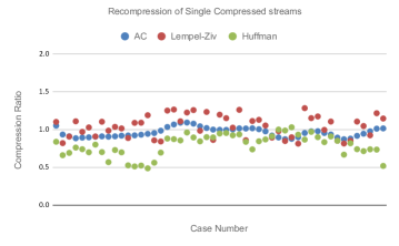
Figure 1: Compression ratio after re-compressing single incoming streams directly using various well-known lossless compressors.

Similarity, we repeated the same re-compression experiments but on collective (i.e. all together) multi-incoming compressed streams. We set 56 streams per experiment. Fig. 2) shows the CR of these experiments, which varies between $0.5-$to$-1.1$ with an average of $0.7$. This is worse than the single re-compression. Hence, the observation from the experiment (B) is that it would also be discouraged to re-compress a collective of compressed streams directly together.

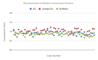
Figure 2: Average compression ratio after re-compressing the multi-incoming compressed streams all together which was very poor (CR is $\leq 1$).

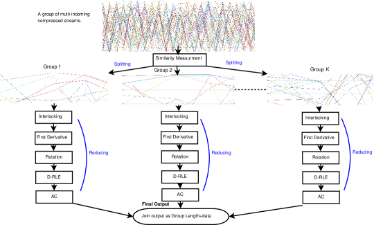
Figure 3: An overview of the steps undertaking in our model where similarity measurement technique used to split the compressed streams. Then, the aggregation and size reduction steps are performed.

IV Our Re-compression Model

A possible way to reduce the noise in the collective compressed streams is to explore the potential similarities among subgroups of these compressed streams and design an interlocking friendly compression algorithm. Therefore, the unsupervised learning technique i.e., K-Means clustering has been used as a similarity measurement to classify the compressed streams into subsets. The streams in every subset have been interlocked followed by the first derivative to reduce the values’ space and increase the redundancy. After that, both BWT and MTF have been applied to rotate and rearrange the readings in a more consecutive format before employing the developed dynamic RLE. Finally, entropy coding is performed. Fig. 3 demonstrates an overview of our proposed model.

IV-A Similarity Measurement - K-Means

K-means [21] is used as a similarity measurement to cluster $n$ observations into $K$ groups and avoid the noise of mixing all together. The main idea is that, let us assume $(x_{1},x_{2},...,x_{n})$ are the $n$ incoming compressed streams where each stream is a d-dimensional vector. K-means will partitions the $n$ streams into $K(\leq n)$ groups $(G_{1},G_{2},..,G_{k})$ by summation of distance functions of each point in the group to $K$ center. The objective is depicted in Eq 1

$$\sum_{i=1}^{k}\sum_{j=1}^{\sigma_{i}}(\left\|x_{i}-\mu_{j}\right\|)^{2}$$ (1)

where $\sigma_{i}$ is the number of data points in the $i^{th}$ group, $\mu_{j}$ is the center of the $i^{th}$ group and $\left\|x_{i}-\mu_{j}\right\|$ is the Euclidean distance between $x_{i}$ and $\mu_{j}$.

The algorithm started by selecting cluster centers $\mu_{j}$. The distance between each reading point $x_{i}$ and $\mu_{j}$ is then calculated. Next, the reading point $x_{i}$ is assigned to $\mu_{j}$ based on the best minimum distance. After that, a new cluster center $\mu_{j}$ is recalculated as shown in Eq. 2

$$\mu_{i}=\left(\frac{1}{\sigma_{i}}\right)\sum_{j=1}^{\sigma_{i}}x_{i}$$ (2)

where $\sigma_{i}$ represents the number of reading points in $i^{th}$ cluster. The distance between $x_{i}$ and $\mu$ is then recalculated. The assignment process will be repeated (See Eq 3), until no further data points need to be reassigned.

$$G_{i}=\left\{x_{p}:\left\|x_{p}-m_{i}\right\|^{2}\leq\left\|x_{p}-m_{j}\right\|^{2}\forall_{j},1\leq j\leq k\right\}$$ (3)

The most crucial part is how centroid points are chosen. Therefore, to avoid the exponential time complexity of the standard algorithm, the idea proposed by Arthur and Vassilvitskii [22] has been used by utilizing a heuristic to find the centroid seeds for the algorithm as follows. Only one random center $\mu$ is uniformly chosen from among the readings. Then, the distance between $x_{i}$ and the closest center (i.e. chosen one) is computed. Next, one of the readings is chosen to be the new center $\mu$ using a weighted distribution probability (See Eq 4). These steps are repeated until k centers are chosen.

$$\frac{d^{2}\left(x_{i},\mu_{p}\right)}{\sum_{\left\{j,x_{j}\in\Re_{p}\right\}}\left(x_{j},\mu_{p}\right)}$$ (4)

where $\Re_{p}$ is the group of all observations nearest to centroid. $\mu_{p}$ and $x_{i}$ belong to $\Re_{p}$.

IV-B Size Reduction

After completing the similarity measurement process, each resultant group is combined and its size will be reduced using the following steps.

IV-B1 Readings Interlocking

Let us assume $G_{i}$ is one of the resultant groups. It has $1,2,...,n$ vectors that represent multiple compressed streams as shown in Eq 5.

$$G_{m,n}=\begin{pmatrix}a_{1,1}&a_{1,2}&\cdots&a_{1,n}\\ b_{2,1}&b_{2,2}&\cdots&b_{2,n}\\ \vdots&\vdots&\ddots&\vdots\\ c_{m,1}&c_{m,2}&\cdots&c_{m,n}\end{pmatrix}$$ (5)

Therefore, these streams will be overlapped to exploit similar features (See Eq 6).

$$a(1,1),b(2,1),...,c(m,1)$$ (6)

To avoid any sharp exponential deviations in the overlapped readings and increase the redundancy, the first derivative is applied as shown Eq 7.

$$f_{d}=[\Upsilon(2)-\Upsilon(1)\Upsilon(3)-\Upsilon()2)...\Upsilon(\Lambda)-\Upsilon(\Lambda-1)]$$ (7)

where $\Upsilon$ represents data points in the combined stream and $\Lambda$ is the latest value.

IV-B2 Burrow Wheeler Transform (BWT)

Based on experimental observations, the resultant values after applying the first derivative reflects that there are high redundancies but in a very scattered format which impedes any size-reduction attempts. Consequently, a well-known transformation technique called BWT is employed to reshuffle the samples which result in a long consecutive and identical sequence. Originally, BWT has been proposed by Michael Burrows and David Wheeler [23] to rearrange text streams into a format that boosts its compressibility by utilizing mechanisms such as MTF and RLE. The advantage of this algorithm is that zero additional overhead needed to reverse it. Basically, the data (i.e. 1 to $n$) is rotated lexicographically. Let us assume $\Omega$ be textual or numerical of symbols group form (i.e. numerical in our algorithm) to be compressed.

$$\Omega=\Omega_{1},\Omega_{2},...,\Omega_{n}$$ (8)

Iteratively, the vector $\Omega$ is rotated to the left which results in a new 2D matrix called $\beta$, as shown in Eq. 9

$$\beta=\begin{pmatrix}\Omega_{1}&\Omega_{2}&\Omega_{3}&\cdots&\Omega_{n}\\ \Omega_{2}&\Omega_{3}&\cdots&\Omega_{n}&\Omega_{1}\\ \Omega_{3}&\cdots&\Omega_{n}&\Omega_{1}&\Omega_{2}\\ \vdots&\vdots&&\ddots&\vdots\\ \Omega_{n}&\Omega_{1}&\Omega_{2}&\cdots&\Omega_{n}-1\end{pmatrix}$$ (9)

From Eq. 9, it is obvious that each rotation of $\Omega$ is represented as a row in $\beta$. These rows are then sorted in ascending order which will generate a new version of the matrix called $\widetilde{\beta}$. Only the last column $C$ of $\beta$ and the original block index $I$ are kept to be used for retrieving the original order. For clear understanding, a portion of the resultant first derivative values are presented in Table I. These samples have been replaced by characters (i.e. represent $\Omega$) for the sake of simplicity. $\beta$ is generated by rotating $\Omega$ for $n$ (i.e. the number of elements) times. The rows of $\beta$ will then be sorted which results in a new form $\widetilde{\beta}$ as depicted in Eq. 10

$$\widetilde{\beta}=\begin{Bmatrix}a&\color[rgb]{0,0,1}\$&a&b&a&a&\color[rgb]{1,0,0}\boldsymbol{b}\\ a&a&b&a&\color[rgb]{0,0,1}\$&a&\color[rgb]{1,0,0}\boldsymbol{b}\\ \color[rgb]{1,0,0}\boldsymbol{a}&\color[rgb]{1,0,0}\boldsymbol{b}&\color[rgb]{1,0,0}\boldsymbol{a}&\color[rgb]{1,0,0}\boldsymbol{a}&\color[rgb]{1,0,0}\boldsymbol{b}&\color[rgb]{1,0,0}\boldsymbol{a}&\color[rgb]{1,0,0}\boldsymbol{\$}\\ a&b&a&\color[rgb]{0,0,1}\$&a&b&\color[rgb]{1,0,0}\boldsymbol{a}\\ b&a&a&b&a&\color[rgb]{0,0,1}\$&\color[rgb]{1,0,0}\boldsymbol{a}\\ b&a&\color[rgb]{0,0,1}\$&a&b&a&\color[rgb]{1,0,0}\boldsymbol{a}\\ \color[rgb]{0,0,1}\$&a&b&a&a&b&\color[rgb]{1,0,0}\boldsymbol{a}\end{Bmatrix}$$ (10)

The last column $C$ and the index I (e.g. 3 in this example) represent the output and used by the decoder to recover the original form by inversing the above steps.

TABLE I: Conversion from Numeric to characters

$\omega$	309	501	309	309	501	309
$Ch$	a	b	a	a	b	a

IV-B3 Move-To-Front (MTF)

Despite the resultant BWT values precisely gathers identical symbols in long runs, these values still sharply vary from very low (e.g. 20 and 21) to much higher numbers (e.g. 4000 and 6000). Consequently, MTF transform is employed to boost the influence of any entropy based encoder (e.g. Arithmetic Coding) to achieve the highest compression rate. MTF is a lightweight mechanism introduced by Ryabko [24] to enhance the low values (e.g. close to zero) probability while minimizing the high values in a given list of data. The basic idea is that the data list symbols are substituted by their positions in a unique list. With this, the long sequential identical symbols will be substituted by as many zeros, whereas a posterior (i.e. not regularly used) symbols will be exchanged by larger values.

TABLE II: MTF of $L=\left[b,b,a,a,a,a,a,a\right]$ and $u=\left[a,b\right]$

$L_{i}$	b	b	a	a	a	a	a	a
$u$	a, b	b, a	b, a	a, b	a, b	a, b	a, b	a, b
$\vartheta$	1	0	1	0	0	0	0	0

Let us assume the BWT resultant list is $L=\left[b,b,a,a,a,a,a,a\right]$ and so its unique list is $u=\left[a,b\right]$ (See Table II). The initial token $L_{0}$ is $b$, and its preceded by one symbol in $u$. Therefore, the digit one is produced in $\vartheta$ and the symbol $b$ is moved to the front of $u=\left[b,a\right]$. The next token $L_{1}$ is $b$ which is the first in $u$, and so the produced value is $0$ and no need to update $u$. These steps are continued until the last token is reached the resultant output will look like $\vartheta=\left[1,0,1,0,0,0,0,0\right]$.

IV-B4 Run Length

The MTF output includes series of identical sequential tokens. Consequently, to exploit this fact, a simple mechanism called run length (RLE) [25] is employed before the entropy encoding. RLE focuses on substituting the similar consecutive symbols by their count. Let $s$ represents a symbol that appears $n$ sequential times in a vector $V$. The $n$ cases are then substituted by $ns$. The $n$ consecutive appearances of the symbol are called run length. For instance, the sequential zeros in $\vartheta=\left[1,0,1,0,0,0,0,0\right]$ will be $\vartheta=\left[1,0,1,0\#5\right]$. However, the observation was that a naive implanting of RLE is not always useful and may increase rather than decrease. This is due to its static nature where each consecutive symbols are replaced even in the case of no repeated tokens occurs. RLE is improved to be a dynamic (by adding 1 bit) based on thresholds $t=t1,t2,..,t_{n}$ that monitor the consecutive occurrences of the symbols.

TABLE III: The message $m$ probability Distribution

Symbol	Probability	Accumulative range
a	0.2	(0.0,0.2)
b	0.3	(0.2,0.5)
c	0.1	(0.5,0.6)
d	0.2	(0.6,0.8)
e	0.1	(0.8,0.9)
f	0.1	(0.9,1.0)

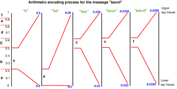
Figure 4: Graphical representation for Arithmetic encoding steps for a message $b,a,c,c,f$

IV-B5 Arithmetic Coding

An entropy coding mechanism called Arithmetic Coding (AC) is ultimately employed in our model to achieve the highest possible compression ratio. AC is a widely-known variable length statistical coding by which repeatedly occurred values are represented with fewer bits whereas less frequently appearing tokens are symbolized with higher bits number [25]. AC proved its superiority in most respects to other well-known entropy algorithms such as Huffman coding. This is due to its succinct representation of the entire message in a single value as a fraction $n$ where $\left(0.0\leq n<1.0\right)$, whereas other algorithms working on separating the input into isolated component tokens and substituting each with a unique code.

The general idea is that after choosing a specific interval, the symbols list will be scanned and based on its tokens probabilities, the ultimate interval will be narrowed.

To demonstrate AC mechanism, let us assume that an entire message $M$ that has a probability distribution as given in Table III. For brevity, a fraction of that message $\tilde{m}=(b,a,c,c,f)$ is encoded (see Fig. 4). The probability boundary is between $(0,1)$. To begin with, due to the occurrence of symbol $b^{\prime}$, the tag value should be in the range $(0.2,0.5)$. After that, the token ${}^{\prime}a^{\prime}$ is appeared, so the present interval between $(0,0.2)$ which will be used to calculate the lower boundary: $w_{n}=l_{n-1}+(w_{n-1}-\rho_{n-1})\times F_{x}(x_{n-1})$ and upper boundary: $\rho_{n}=w_{n-1}+(\rho_{n-1}-\rho_{n-1})\times F_{x}(x)$. $F_{x}$ is the frequency accumulation.

The resultant tag values of symbols sequence ’ba’ are $(0.2,0.26)$. This will continue for the full message in an accumulative manner. The ultimate tag values output has been summed up in Fig. 4. The average of both the final upper and lower tags $\frac{w_{n}+\rho_{n}}{2}=\frac{0.23354+0.2336}{2}=0.23357$ represents the compressed value and will be transformed into binary.

The decoder side requires both the average value and the message probabilities. Subsequently, it proceeds through similar steps but in an inverse manner where the probability accumulation is used to find the symbols.

V Decompression and Recovery

The recovery process is almost similar to the steps stated above but in the opposite manner. It begins by Arithmetic decoding followed by RLE if needed (i.e. based on the conditions mentioned in Section IV-B4). Then, MTV and BWT are applied respectively. The output represents the derivative values and so their inverse process is employed to reconstruct the actual symbols. These symbols are the compressed streams in an interlocking way. From that, they are disunited to their single compressed streams and so their original format is recovered in a lossless format.

VI Evaluation

Various matrices are used to examine the effectiveness of our lossless size reduction model.

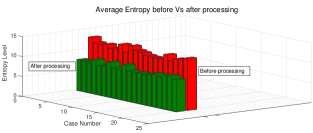
Figure 5: Comparison between the average entropy calculated from the compressed streams before and after aggregation and processing.

VI-A Silhouette Measurement

To validate the coherence of the used similarity measurement clustering techniques, a mathematical model called Silhouette is used. It is a graphical representation technique proposed by Peter J. Rousseeuw [26] that proves the consistency within the data cluster and clearly reflects the correlation of the objects within that group. The Silhouette model produces a value in the range of $-1$ to $1$, in which the higher the value, the more the object is well matched to that group and vice versa. Let us assume $n$ vectors are clustered into $K$ groups using a similarity measurement model (e.g. $K$-means). For each group $G$, $x(i)$ represents the average dissimilarity (i.e. distance ) of $i$ within the group (i.e. the least the value, the better the matching). Also, let $y(i)$ be the lowest dissimilarity of $i$ within the group. With this, silhouette $s$ can be defined as follows.

$$s(i)=\frac{y(i)-x(i)}{\max\{x(i),y(i)\}}$$ (11)

$$s(i)=\begin{cases}1-\frac{x(i)}{y(i)},&\text{ if }x(i)<y(i)\\ 0,&\text{ if }x(i)=y(i)\\ \frac{x(i)}{y(i)}-1&\text{ if }x(i)>y(i)\end{cases}$$ (12)

From 11 and 12, it can be derived that $-1\leq s(i)\leq 1$.

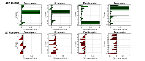
Figure 6: Comparison between the consistency among the clusters by changing two parameters. These are the number of clusters and the similarity measurement technique (i.e. K-means vs Rand).

VI-B Theoretical Entropy

The entropy of a signal in the information theory field represents the lowest bit-rate (i.e. the optimum compression assumed) needed for transmitting this signal [27]. Consequently, to monitor the influence of preprocessing the compressed streams in our model, the theoretical entropy is measured for every smart meter compressed stream before and after employing our model. After that, the quantitative calculation comparison is performed between the theoretical entropy and the accomplished size reduction ratio. Let us assume a compressed incoming stream consisting of the symbol points $d[1],d[2],...,d[N]$. The optimum likelihood entropy (i.e. in bits) is calculated as

$$H(d)\triangleq-\sum_{i\in\mathbb{R}(d)}\widehat{p}(i)\log_{2}(\widehat{p}(i))$$ (13)

$$\widehat{p}(i)\triangleq\frac{1}{N}\sum_{n=1}^{N}\delta_{i}(d[n])$$ (14)

$$\delta_{i}(d[n])\triangleq\begin{cases}1,&\text{ if }d[n]=i\\ 0,&else\end{cases}$$ (15)

where $\widehat{p}(i)$ is the experimental probability of $i\in\mathbb{R}$ and $\mathbb{R}(d)$ represents the range of $d$. The smallest entropy (i.e. optimum case) happens when all $d$ symbols are equal, which results in $H_{min}=-1\log_{2}(1)=0$.

On the other hand, the worst-case (i.e. maximum entropy) happens when each symbol in $\mathbb{R}$ occurs at the somehow similar frequency $1/\mathbb{R}$, in which $|\mathbb{R}|$ reflects the original elements in $\mathbb{R}$ (See Eq. 16).

$$H_{\max}=-\sum_{i\in\mathbb{R}}\frac{1}{|\mathbb{R}|}\log_{2}(\frac{1}{|\mathbb{R}|})=\log_{2}|\mathbb{R}|.$$ (16)

VII Experimental Ratio

The compression ratio (CR) is the essential benchmark to measure any proposed compression model empirically. Let us symbolize the original compressed streams block $O$ (i.e. it’s unit in bit or byte) and the resultant re-compressed symbols $R$. Consequently, the experimental CR in the results section is measured as $CR=\frac{O}{R}$. The widely-known leading power quality storage standard for electric waveforms power system utilized in most of smart meters called PQDIF (Power Quality Data Interchange Format) has been employed in producing the multi compressed streams dataset. Every Reading represented as 16 bit and the typical suggested block size is used which is about 1500 readings. The entropy-based compression model published in [13] is employed which proven to give the optimum lossless compression ratio $3.8:1$.

TABLE IV: Compression ratio

Record	Cluster No	Static RLE (Rand)	Static RLE(Kmeans)	Dynamic RLE (Rand)	Dynamic RLE (Kmeans)
1	2	1.03	0.40	1.30	1.75
2	2	1.08	0.31	1.36	1.73
3	2	1.12	1.46	1.31	1.77
4	2	1.01	1.52	1.30	1.73
5	4	1.07	1.53	.35	1.81
6	4	1.10	1.38	1.30	1.76
7	4	1.18	1.53	1.33	1.81
8	4	1.12	1.63	1.31	1.83
9	6	1.08	1.59	1.39	1.90
10	6	1.12	1.43	1.33	1.90
11	6	1.20	1.55	1.35	1.98
12	6	1.17	1.67	1.33	1.98
13	8	1.05	1.69	1.40	2.11
14	8	1.16	1.55	1.44	2.13
15	8	1.23	1.67	1.35	2.10
16	8	1.29	1.77	1.42	2.19
17	10	1.10	1.63	1.36	1.94
18	10	1.15	1.43	1.40	1.95
19	10	1.21	1.60	1.38	2.04
20	10	1.19	1.70	1.40	2.03
21	12	1.04	1.51	1.31	1.85
22	12	1.11	1.41	1.33	1.89
23	12	1.20	1.58	1.36	1.97
24	12	1.10	1.66	1.42	2.04
Average		1.13	1.55	1.36	1.92

VIII Implementations

VIII-A Datasets

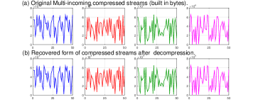
Figure 7: 4 examples of compressed watts consumptions’ readings collected from different homes: (a) Direct plot of single compressed streams form, and (b) Plot of these streams after dis-aggregation and recovery.

The Laboratory for Advanced System Software collected and published a detailed smart meters datasets as a part of a project called ”Smart” [28, 29]. These datasets have been thoroughly used in our experiments. The datasets entries represent a periodical (i.e. per minutes) readings from three houses for more than three months. Also, a detailed electricity consumption (i.e. per minutes) from about 400 anonymous premises for $(24\times 30\times 3)hrs$ is provided. Our recent Gaussian based compression [13] is applied on every single stream, to generate the multi-incoming compressed streams as explained in the evaluation Section VI. The compressed streams are laid out as the bed-test in all of our experiments.

VIII-B Experiments and Results

Our prime executed experiments will be done at the operation centers or cloud level after receiving an overwhelming amount of compressed streams from a huge number of premises. The experiments can be categorized into (a) similarity measurements, interleaving and size reduction processes, and (b) an original format recovery. Both categories are designed in such a way that can be done in parallel to take advantage of cloud power. To obtain unbiased outcomes, all compressed streams mentioned above have been employed in our model.

For brevity in this paper, the results have been summarized as follows. Fig. 6 reflects the superiority (more group cohesiveness $>$0) as a graphical comparison (i.e. using Silhouette benchmark) between our similarity measurement using $K-means$ against a random agnostic grouping. Secondly, Fig. 5 shows a comparison between the average entropy calculated from the compressed streams of few random streams together vs a processed cluster after using our model. The entropy has been noticeably reduced from around 13 bits into 7 bits. Thirdly, Table IV presents the exact CR achieved from the 4 configurations starting from Random Cluster and Static RLE to Kmeans cluster with Dynamic RLE. This proves the feasibility of improving CR using clustering and dynamic RLE. Fourthly, Fig 8 shows the average of CR ratio obtained from the above four groups (i.e. 8 Kmeans clusters + dynamic RLE is the optimum). Finally, Fig 7 shows an example of a plot of various original compressed streams before and after the aggregation and size reduction process.

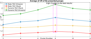
Figure 8: The average of re-compression ratio of the four groups examined in Table IV which shows the best combination of our technique parameters.

VIII-C Discussion

Recall, the main question drives this work: Can the multi-incoming smart meter compressed streams be re-compressed? By exploring the potential similarities in various compressed streams using a similarity measurement techniques, our model demonstrated that it is possible to re-compress multi-incoming compressed streams. We achieved up to 2:1 size reduction level in the optimum setting and 1.9:1 in average. This means every 1Gigabyte byte can be reduced to $\sim$500 Megabyte. This has been emphasized theoretically by comparing the entropy before and after our technique (See Fig. 5) and experimentally as presented in Table IV. The scalability impact in the number of compressed streams that goes into similarity measurement along with the number of samples per stream before the initial compression remain to be addressed in our future work.

IX Conclusion

In this paper, a novel lossless re-compression algorithm was introduced to prove the possibility of reducing the size of the already compressed waveform smart meter readings. The main target was preprocessing the data to enhance the entropy. This is successfully achieved by employing K-Means clustering as similarity measurement to classify the compressed streams into subsets to reduce the effect of uncorrelated compressed streams. The tokens of every subset have been interlocked followed by the first derivative to reduce the values’ space and boost the redundancy. After that, two rotation steps have been applied to rearrange the symbols in a more consecutive format before employing dynamic RLE. Finally, entropy coding is performed. Both mathematical and empirical experiments proved the possibility of enhancing the entropy (i.e. almost reduced by half) and the resultant size reduction (i.e. up to 50%).

References

- [1] Vehbi C Gungor, Bin Lu, and Gerhard P Hancke. Opportunities and challenges of wireless sensor networks in smart grid. Industrial Electronics, IEEE Transactions on, 57(10):3557–3564, 2010.
- [2] CIGRE. D2-21 cigre working group d2.21, wg. broadband plc applications, http://www.cigre.org/what-is-cigre, accessed: 15.01.2020.
- [3] Vehbi C Güngör, Dilan Sahin, Taskin Kocak, Salih Ergüt, Concettina Buccella, Carlo Cecati, and Gerhard P Hancke. Smart grid technologies: communication technologies and standards. Industrial informatics, IEEE transactions on, 7(4):529–539, 2011.
- [4] Michel P Tcheou, Lisandro Lovisolo, Moisés Vidal Ribeiro, Eduardo AB da Silva, Marco AM Rodrigues, Joao Marcos Travassos Romano, and Paulo SR Diniz. The compression of electric signal waveforms for smart grids: state of the art and future trends. Smart Grid, IEEE Transactions on, 5(1):291–302, 2014.
- [5] Jiaxin Ning, Jianhui Wang, Wenzhong Gao, and Cong Liu. A wavelet-based data compression technique for smart grid. Smart Grid, IEEE Transactions on, 2(1):212–218, 2011.
- [6] Norman CF Tse, JohnY C Chan, Wing-Hong Lau, Jone TY Poon, and LL Lai. Real-time power-quality monitoring with hybrid sinusoidal and lifting wavelet compression algorithm. Power Delivery, IEEE Transactions on, 27(4):1718–1726, 2012.
- [7] Michel P Tcheou, Lisandro Lovisolo, Eduardo AB da Silva, Marco AM Rodrigues, and Paulo SR Diniz. Optimum rate-distortion dictionary selection for compression of atomic decompositions of electric disturbance signals. Signal Processing Letters, IEEE, 14(2):81–84, 2007.
- [8] Moisés V Ribeiro, Seop Hyeong Park, João Marcos T Romano, and Sanjit K Mitra. A novel mdl-based compression method for power quality applications. Power Delivery, IEEE Transactions on, 22(1):27–36, 2007.
- [9] Alsharif Abuadbba and Ibrahim Khalil. Wavelet based steganographic technique to protect household confidential information and seal the transmitted smart grid readings. Information Systems (2014)., 2014.
- [10] J. C. S. de Souza, T. M. L. Assis, and B. C. Pal. Data compression in smart distribution systems via singular value decomposition. IEEE Transactions on Smart Grid, (99):1–1, 2015.
- [11] J. E. Tate. Preprocessing and golomb -rice encoding for lossless compression of phasor angle data. IEEE Transactions on Smart Grid, 7(2):718–729, March 2016.
- [12] Sharda Tripathi and Swades De. An efficient data characterization and reduction scheme for smart metering infrastructure. IEEE Transactions on Industrial Informatics, 14(10):4300–4308, 2018.
- [13] Alsharif Abuadbba, Ibrahim Khalil, and Xinghuo Yu. Gaussian approximation based lossless compression of smart meter readings. IEEE Transactions on Smart Grid, 2017.
- [14] Surya Santoso, Edward J Powers, and WM Grady. Power quality disturbance data compression using wavelet transform methods. Power Delivery, IEEE Transactions on, 12(3):1250–1257, 1997.
- [15] Saroj K Meher, AK Pradhan, and G Panda. An integrated data compression scheme for power quality events using spline wavelet and neural network. Electric power systems research, 69(2):213–220, 2004.
- [16] Ganapati Panda, PK Dash, Ashok Kumar Pradhan, and Saroj K Meher. Data compression of power quality events using the slantlet transform. Power Delivery, IEEE Transactions on, 17(2):662–667, 2002.
- [17] Ömer Nezih Gerek and Dogan Gökhan Ece. Compression of power quality event data using 2d representation. Electric Power Systems Research, 78(6):1047–1052, 2008.
- [18] Jan Kraus, Tomas Tobiska, and Viktor Bubla. Loooseless encodings and compression algorithms applied on power quality datasets. In Electricity Distribution-Part 1, 2009. CIRED 2009. 20th International Conference and Exhibition on, pages 1–4. IET, 2009.
- [19] Dahai Zhang, Yanqiu Bi, and Jianguo Zhao. A new data compression algorithm for power quality online monitoring. In Sustainable Power Generation and Supply, 2009. SUPERGEN’09. International Conference on, pages 1–4. IEEE, 2009.
- [20] Jan Kraus, Pavel Štépán, and Leoš Kukačka. Optimal data compression techniques for smart grid and power quality trend data. In Harmonics and Quality of Power (ICHQP), 2012 IEEE 15th International Conference on, pages 707–712. IEEE, 2012.
- [21] Stuart Lloyd. Least squares quantization in pcm. IEEE transactions on information theory, 28(2):129–137, 1982.
- [22] David Arthur and Sergei Vassilvitskii. k-means++: The advantages of careful seeding. In Proceedings of the eighteenth annual ACM-SIAM symposium on Discrete algorithms, pages 1027–1035. Society for Industrial and Applied Mathematics, 2007.
- [23] M. Burrows and D. J. Wheeler. A block-sorting lossless data compression algorithm. Digital SRC Research Report, (124), 1994.
- [24] B Ryabko. Data compression by means of a ”book stack”. Problems of Information Transmission, 16(4):265–269, 1980.
- [25] David Salomon. Data Compression: The Complete Reference. Springer-Verlag New York, 2004.
- [26] Peter J Rousseeuw. Silhouettes: a graphical aid to the interpretation and validation of cluster analysis. Journal of computational and applied mathematics, 20:53–65, 1987.
- [27] C. E. Shannon. A mathematical theory of communication. The Bell System Technical Journal, 27(4):623–656, Oct 1948.
- [28] Sean Barker, Aditya Mishra, David Irwin, Emmanuel Cecchet, Prashant Shenoy, and Jeannie Albrecht. Smart project. http://traces.cs.umass.edu/index.php/Smart/Smart, 2012.
- [29] Sean Barker, Aditya Mishra, David Irwin, Emmanuel Cecchet, Prashant Shenoy, and Jeannie Albrecht. Smart*: An open data set and tools for enabling research in sustainable homes. SustKDD, August, 2012.