Unsupervised clustering of Roman pottery profiles from their SSAE representation

Abstract

In this paper we introduce the ROman COmmonware POTtery (ROCOPOT) database, which comprises of more than 2000 black and white imaging profiles of pottery shapes extracted from 11 Roman catalogues and related to different excavation sites. The partiality and the handcrafted variance of the shape fragments within this new database make their unsupervised clustering a very challenging problem: profile similarities are thus explored via the hierarchical clustering of non-linear features learned in the latent representation space of a stacked sparse autoencoder (SSAE) network, unveiling new profile matches. Results are commented both from a mathematical and archaeological perspective so as to unlock new research directions in the respective communities.

1 Introduction

Our ability to interpret an archaeological site as belonging to a specific period rests on our capacity to assign a chronology to the material culture found in it, ranging from fixed structures to movable objects. Thanks to their relative resilience against decay combined with their specific underlying patterns of production, distribution and consumption, ceramic vessels (pottery) – whether fragmented (i.e. potsherds) or intact – represent some of the most common finds recovered during archaeological fieldwork. Individual pots and potsherds are usually recorded as 2D profiles and, in consideration of their morphological features (e.g. shape of the rim or the base), are then gathered in systematic catalogues (corpora), where patterns of similarity are used to establish relationships, in terms of function, chronology or both [41].

Within Roman archaeology specifically (albeit not exclusively), fundamental significance has been ascribed to those ceramic classes more closely associated with long-distance trade and contact, namely trade containers (amphorae) and high-quality tableware pots (fineware). However, these were middle-range commodities that did not reach all levels of society in the same way, and, furthermore, their supply varied enormously over time and space. Indeed, some sites might have had limited or no access to this range of objects, and such notable absence in the archaeological record might be taken to indicate their abandonment at a time when – in fact - they were in full occupation (i.e. reduced archaeological visibility). In contrast, ordinary table- and kitchen-ware (commonware) were considerably cheaper and mainly supplied within a local/regional network of distribution. As a result, they almost invariably constitute the bulk of pottery finds at almost every Roman site. Even though one would expect them to provide a most effective baseline for the dating (and more general interpretation) of Roman sites anywhere, their huge range of forms, poorly defined chronologies and scattered provenance have made their study so challenging (and so little promising) that many have favoured the analysis of the far more standardised and easily recognisable fineware and amphorae.

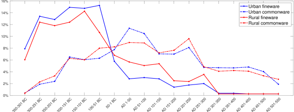
Nevertheless, when a special effort is made to include a comprehensive study of commonware sherds, resulting interpretations can dramatically change. This was neatly shown by a recent analysis of the chronological distribution of potsherds recovered from the Roman town of Interamna Lirenas and from across its surrounding countryside [33]. Whereas traditional reliance on fineware and amphorae had outlined a trajectory of precocious demographic decline (already in progress by the late 1st century BC), the widespread presence of commonware shows a considerably more gradual process of growth, in fact peaking in the course of the 1st century AD, with little or no sign of decline until about two centuries later, see Figure 1. There can be no doubt that the study of commonware should be a priority within (Roman) material culture studies. However, this does not make the obstacles which archaeologists have to face any less real. What is indeed needed is to organise and classify this vast and varied body of evidence in a way which is considerably more effective and less time-consuming than it currently is.

Figure 1: Percentage distribution of fineware/amphorae (continuous line) and commonware (dashed line) potsherds in urban (blue) and rural (red) environment.

Contributions.

The contribution of this paper is two-fold. Firstly, we detail about the creation of a database of Roman commonware pottery profiles from Central Tyrrhenian Italy, called ROman COmmonware POTtery (ROCOPOT) and containing 2D imaging profiles (in black and white) with metadata extrapolated from different catalogues and excavation sites. Secondly, we propose an unsupervised machine learning workflow for hierarchically clustering the pottery profiles by learning their features in the latent space of stacked sparse autoencoders. Our approach can thus unveil different layers of granularity and permits to discover unexpected subclasses since no comprehensive classification or ground truth is existing on these shapes. Our stated aim is to improve the classification performed by archaeologists on available corpora separately by effectively combining them into one all-encompassing database, with the resulting clustering patterns illuminating possible new morphological and chronological relationships and serving as an additional tool for archaeologists to improve their understanding of the chronology, function and development of both pots and sites over time. Whereas other similar projects have attempted to develop automated procedures for the correct identification of potsherds (i.e. establishing a relationship between what is newly found and the published 2D profiles), our aim is to bring an order into the database itself that facilitates the archaeological classification workflow. The complete pipeline, from archaeological fieldwork to our contributions, is reported in Figure 2.

Figure 2: Summary of our contributions from the production of archaeological corpora.

Related works.

Shape recognition, classification and matching, both with complete and partial data, are well-established problems in the computer vision and mathematical communities but for settled databases of thousands of images or shapes, e.g. [7, 34, 48]. In the recent years, “Cultural Heritage Imaging Science” became a research field of increasing popularity bringing together experts from museum institutions, history of art, physics, chemists, computer vision and mathematics departments for tackling cross-discipline challenging applications; however, few dedicated databases emerged in the literature, mainly related to collection of paintings and associated tasks, e.g. for object or people detection [15, 24, 25], style recognition [4] and many more, see the survey in [22].

Relevant works for matching 2D shapes are based on similarities of boundaries [16, 54] or skeletons [47], homeomorphic transformations based on size functions [17], geodesic calculus for image morphing [45], axiomatic criteria for deformable shapes [6] or comparison of invariant image moments [32, 36, 38, 63]. In particular, invariant shape descriptors are detailed in [8] for clustering similar shapes together while still it remains open the question about the meaningfulness of the obtained clusters. For 3D surfaces (with triangular meshes) or volumes (with voxels), remarkable results are also obtained via scale invariant descriptors based on the eigen-decomposition of the Laplace–Beltrami operator, e.g. the Heat Kernel Signature and its variants [35, 43, 53].

For the targeted application of this paper, even fewer databases are public available [26, 56, 57], with focus on their automatic digitisation, shape extraction and visual presentation [2] or the clustering of a-priori selected geometric shape features into similar classes, e.g. by comparing curve skeletons [42], shape boundaries [49], shape descriptors [46] or employing Generalised Hough Transform distance measures (in the case of petroglyphs, similar to our images) [62] and other a-priori topological features (e.g. pixels height and width, area, circularity, rectangularity, diameters or steepness indexes) [13, 27] or comparison with template primitives [30]. In [3] fragments and nodal points are also extracted from complete 3D models in view of a supervised deep learning approach starting from complete profiles. In contrast, our approach for the feature extraction is totally unsupervised and based on the latent representation space of stacked sparse autoencoders [39]: this approach is motivated by the high availability of just fragments and the necessity to not be biased on features manually selected.

In pattern recognition, hierarchical clustering is a non-parametric yet versatile unsupervised approach for unveiling inherent structures in data or observed features, ordered in a tree called dendrogram [18]. The method is based on the recursive partitioning of the data into clusters of (increasing or decreasing) cardinality, based on the minimisation of a certain cost function that promotes the separability of the data features [14]. Despite hierarchical clustering methods are easy to implement, they are often tuned to the application at hand, with an external evaluation of the results by the experts in the applied field [58]. Specifically to Roman pottery profiles, our approach for an unsupervised hierarchical clustering is in line with the promising works in [27, 31, 49, 62], where, on top of that, we automate the cluster merging rule based on the best cophenetic coefficient score [51]. Finally, we leave the coherency check of our clusters to specialist archaeologists.

Organisation of the paper.

The paper is organised as follows: in Section 2 we describe the creation of the ROman COmmonware POTtery (ROCOPOT) database; in Section 3 we detail about the tools used for clustering our shapes by means of hierarchical clustering of the learned shape features with a stacked sparse autoencoder (SSAE) network; in Section 4 we present and discuss our results.

2 The ROCOPOT Database

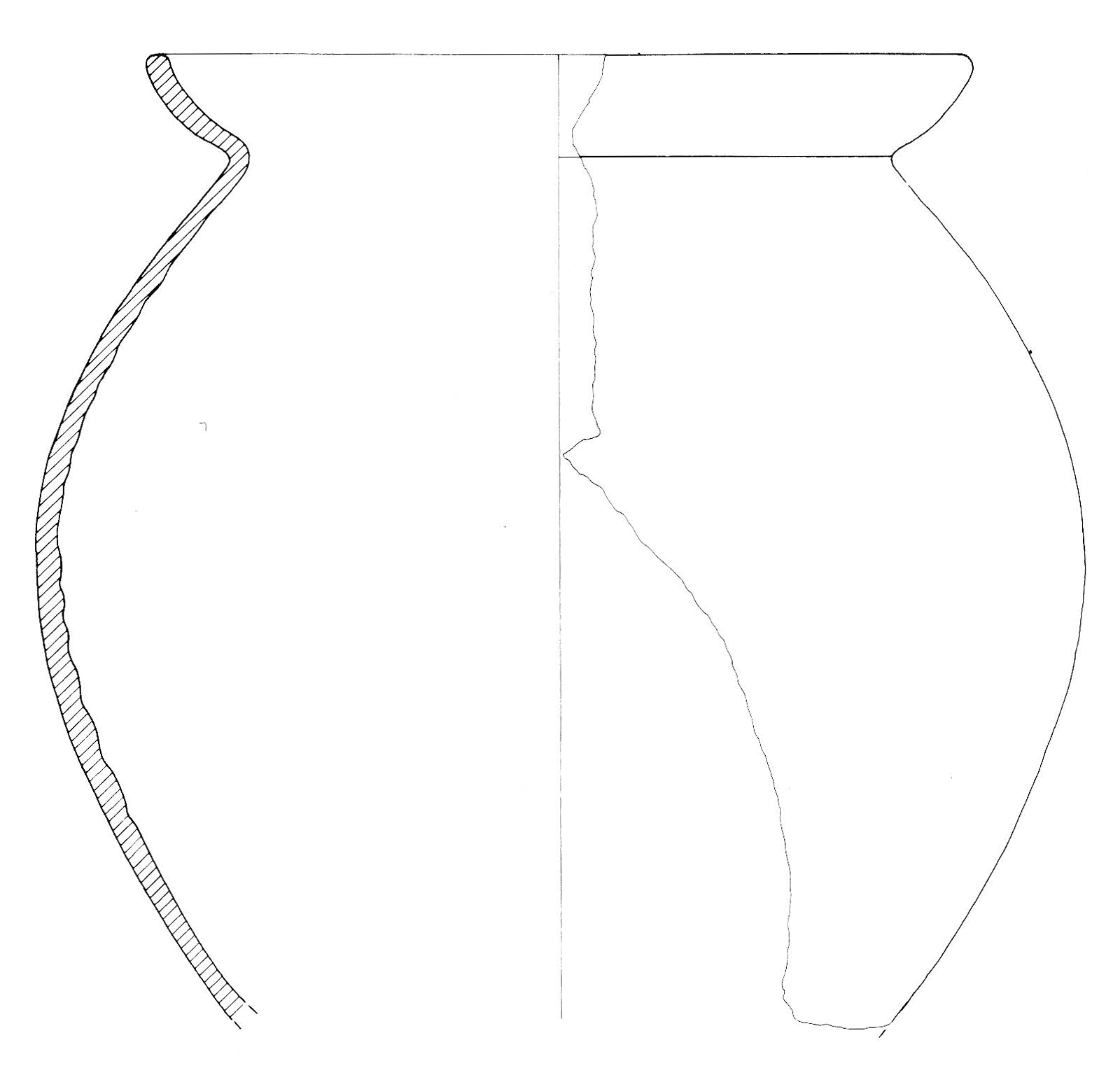
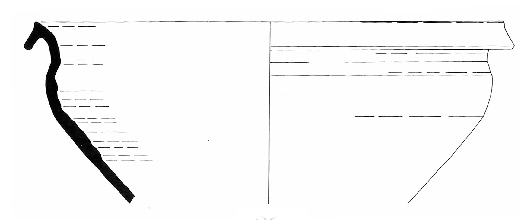
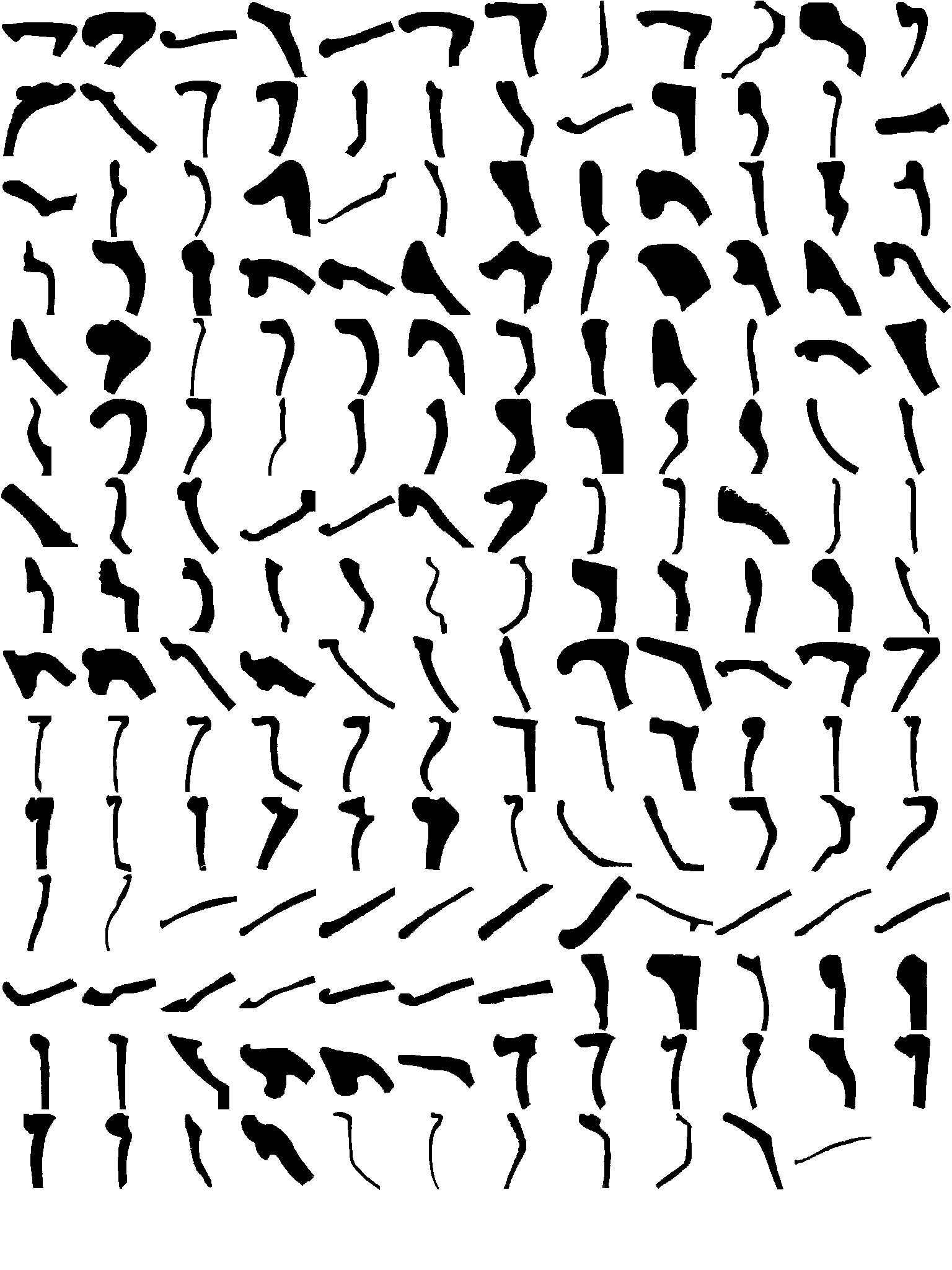
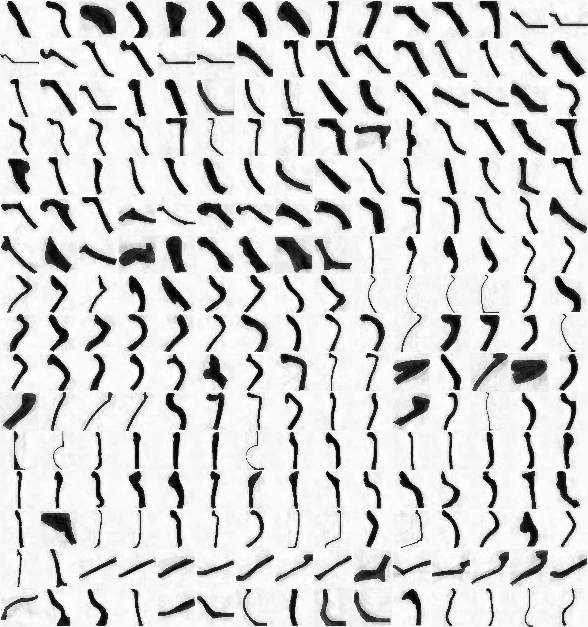
The ROman COmmoware POTtery (ROCOPOT) database described in this paper comprises of 2475 black and white images related to shape profiles extracted from fragments of commonware Roman pottery, as catalogued in a series of corpora [19, 20, 61, 21, 12, 11, 44, 9, 5, 10, 1]. In this work we present the version 1.0 of our database as future extensions are planned. Since the original profiles can be composed of multiple intact parts, the specialists in our project refined the database identifying a total of 231 Bases, 278 Handles, 2103 Rims and 248 Rims with Handles. All of these profiles are black and white images, scanned at 300dpi from the original catalogue and saved in the lossless .png format with an image identification string name of the form IDCAT-PAGNUM.FIGID.png, where IDCAT, PAGENUM pectively, the abbreviation of the catalogue, the page number and the name of the figure where the profile appears. This labelling choice permits a fast inspection of the clustering results by just looking at the filenames as similar profiles from each site tend to be grouped together within the individual catalogues. The details of our database are summarised in Table 1, highlighting the IDCAT, the bibliographic reference, the publication year, the chronology and the archaological site, as well as the number of available profiles: (O)riginals, (B)ases, (H)andles, (R)ims and Rims with Handles (RW).

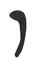
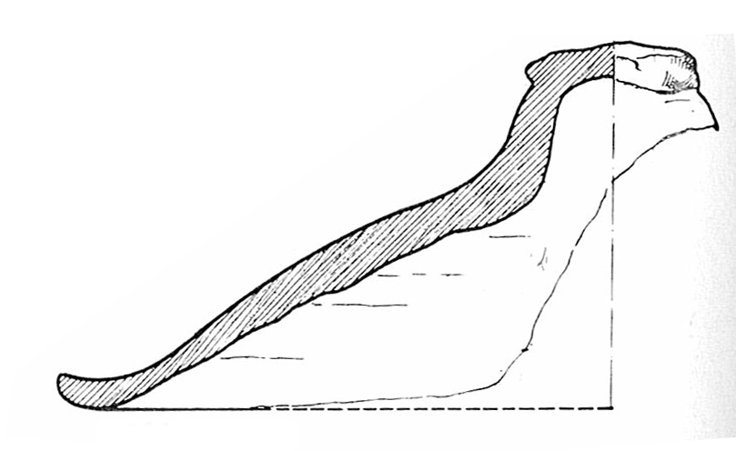
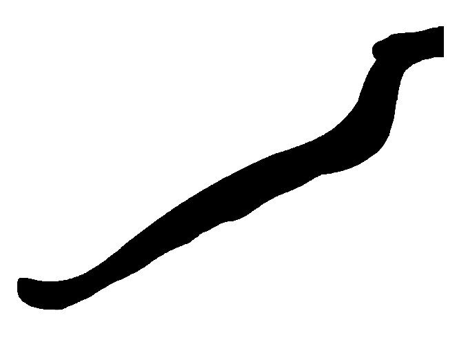
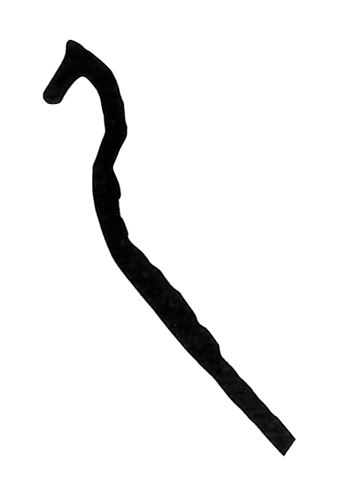
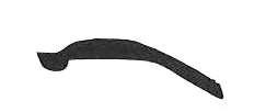
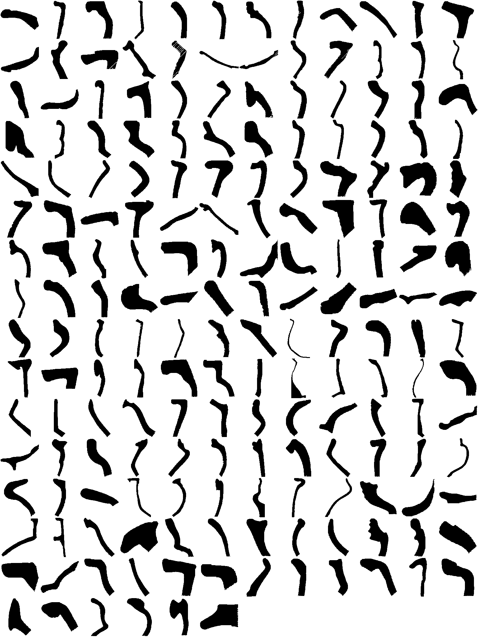
However, all the extracted profiles require a further polishing step so as to make them uniformly represented in the image space before the feature extraction. As a matter of example, in Figure 4 we report common situations when extracting the “Rims”, e.g. the separation of the rim from the template (Figure 3(a)), the fill in of relevant portions with black colour intensity (Figure 3(b) and 3(c)), the cleaning of scanned contours from ageing phenomena and the removal of undesired handles (Figure 3(d) and 3(e)). The expertise of specialist archaeologists is of vital importance at this stage so as to prevent incorrect digitisation of profiles. As an example, the case in Figure 3(f) provides a clear situation where the horizontal features plays a role: if such shape had been rotated clockwise by $90^{\circ}$ degrees, than it would have matched with a different cluster.

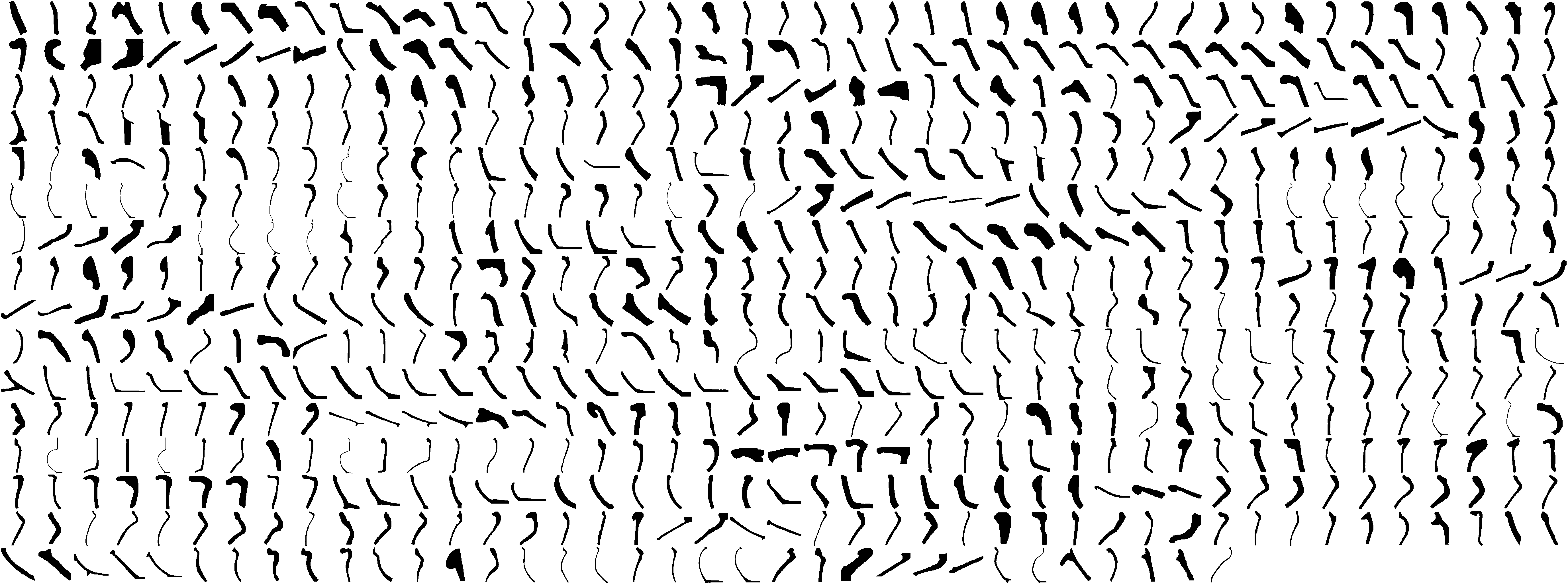
Finally, we make the different profiles comparable by resizing them to a size of 128$\times$128 pixels, without distorting the aspect ratio, see Figure 4: this normalisation is essential in view of the feature extraction with sparse autoencoders.

(a) DYS76-3.CF39

(b) POHL70-55.38

(c) CT84-99.1 CE 2083 3a

(d) DUN64-7.3

(e) ROB97-220.32

(f) DYS76-17.16IV69

Figure 3: Shape preprocessing. Subfigures: original (left) and extracted (right) shape.

(g) DUN64

(h) DUN65

(i) POHL70

(j) DYS76

(k) CT84

(l) CM91

(m) ROB97

(n) OSTIA1

(o) OSTIA2

(p) OSTIA3

(q) OSTIA4

Figure 4: Roman Pottery database v1.0: catalogues with (R)ims shape profiles.

Table 1: Details of the Roman Pottery database v1.0, with number of (O)riginal shapes and their (B)ases, (H)andles, (R)ims and Rims with Handles (RH).

IDCAT	Ref.	Year	Shapes					Chronological range	Site
(catalogue abbreviation)			O	B	H	R	RH
DUN64	[19]	1964	245	13	35	217	37	50 BC - 26 BC	Sutri
DUN65	[20]	1965	127	13	11	107	9	150 BC - 1 BC	Sutri
POHL70	[61]	1970	182	3	9	179	22	200 BC - AD 140	Ostia
DYS76	[21]	1976	814	109	62	679	46	350 BC - AD 335	Cosa
CT84	[12]	1984	269	28	26	240	14	700 BC - AD 100	Pompei
CM91	[11]	1991	43	4	10	39	4	100 BC - AD 200	La Celsa
ROB97	[44]	1997	132	10	21	120	13	AD 101 - AD 635	Monte Gelato
OSTIA1	[9]	1968	168	26	45	120	42	AD 101 - AD 500	Ostia
OSTIA2	[5]	1970	175	20	19	142	24	AD 51 - AD 150	Ostia
OSTIA3	[10]	1973	230	32	31	186	23	AD 51 - AD 500	Ostia
OSTIA4	[1]	1977	90	13	9	74	14	AD 251 - AD 425	Ostia
ALL			2475	231	278	2103	248

3 Proposed approach

After the preprocessing step is carried out, we proceed with the main idea to learn the low-dimensional representation of the shape profiles in our database with sparse autoencoders (SAE) in order to hierarchically cluster the images based on a reduced number of features. Note that the combination of these two approaches makes our workflow totally unsupervised, a key assumption for questioning the established classification in archaeological corpora and unveiling new clustering patterns. For the sake of completeness, we are going to detail in the next subsections the main concepts of these two tools.

Sparse Autoencoders.

The first step is to produce a low dimensional set of features that is able to represent the shapes in the database at their best. Instead of fixing a-priori the quality of the shape features (e.g. the diameter, the ballness, the elongation, the area, the perimeter and many more), we decided to learn the shape representation in a reduced dimensional space of fixed dimension. In this sense, sparse autoencoders are powerful tools as they can be interpreted as a non-linear version of the principle component analysis.

In machine learning, a sparse autoencoder (SAE) is an artificial neural network trained for replicating its input $\bm{u}\in\mathbb{R}^{d}$ at its output $\widehat{\bm{u}}\in\mathbb{R}^{d}$, with $d>0$, by means of back-propagating the reconstructed result so as to learn the input representation onto a smaller dimensional space of neurons via the optimisation of an error measure function called loss function. Here, the sparsity assumption forces the neurons to specialise on few data. In other words, an autoencoder is designed to learn the identity function of the input, see [39]. An autoencoder is composed by two main functions, called encoder and decoder. The encoder is dedicated to the dimensional reduction of the input to the latent subspace, from which the decoder reconstructs the output. More advanced stacked sparse autoencoders (SSAE) [59] are neural networks composed of multiple SAE, where the output of the hidden layer of one autoencoder is inputted to the next autoencoder: this strategy is promising when learning high-level features [60]. In what follows, we detail the main concepts behind SSAE.

Let $\ell=0,\dots,L$ be a variable indexing the layer level up to level $L>0$ and let $(k_{\ell})_{\ell=0}^{L}$ be a monotonic decreasing numeric sequence, with $k_{0}=d$ and $k_{\ell}$ indicating the number of neurons that can be activated at any fixed layer $\ell>0$. For $L=1$, the single-layer encoder network is composed by an encoder map $f^{(1)}:\mathbb{R}^{k_{0}}\to\mathbb{R}^{k_{1}}$ defined as $\bm{v}^{(1)}=f^{(1)}(\mathbf{W}^{(1)}\bm{u}+\bm{b}_{\text{e}}^{(1)})$ with weights $\mathbf{W}^{(1)}\in\mathbb{R}^{k_{1}\times k_{0}}$ and a bias vector $\bm{b}_{\text{e}}^{(1)}\in\mathbb{R}^{k_{1}}$, and a decoder map $g^{(1)}:\mathbb{R}^{k_{1}}\to\mathbb{R}^{k_{0}}$ defined as $\widehat{\bm{u}}=g^{(1)}(\mathbf{W}^{(1),\mathrm{T}}\bm{v}^{(1)}+\bm{b}_{\text{d}}^{(1)})$ with weights $\mathbf{W}^{(1),\mathrm{T}}\in\mathbb{R}^{k_{0}\times k_{1}}$, $(\,\cdot\,)^{\mathrm{T}}$ indicates the transpose operation and bias vector $\bm{b}_{\text{d}}^{(1)}\in\mathbb{R}^{k_{0}}$. For $L>1$, the multi-layer autoencoder network is based on the encoder-decoder strategy iterated for $L$ layers: for example, in a two layers strategy the output $\bm{v}^{(1)}$ of $f^{(1)}$ is concatenated with the encoder $f^{(2)}:\mathbb{R}^{k_{1}}\to\mathbb{R}^{k_{2}}$ via $\bm{v}^{(2)}=f^{(2)}(\mathbf{W}^{(2)}\bm{v}^{(1)}+\bm{b}_{\text{e}}^{(2)})$, with weights $\mathbf{W}^{(2)}\in\mathbb{R}^{k_{2}\times k_{1}}$ and bias vector $\bm{b}_{\text{e}}^{(2)}\in\mathbb{R}^{k_{2}}$, and a decoder map $g^{(2)}:\mathbb{R}^{k_{2}}\to\mathbb{R}^{k_{1}}$ via $\widehat{\bm{v}}^{(1)}=g^{(2)}(\mathbf{W}^{(2),\mathrm{T}}\bm{v}^{(2)}+\bm{b}_{\text{d}}^{(2)})$, with weights $\mathbf{W}^{(2),\mathrm{T}}\in\mathbb{R}^{k_{2}\times k_{1}}$ and bias vector $\bm{b}_{\text{d}}^{(2)}\in\mathbb{R}^{k_{1}}$. For a generic vector $\bm{z}\in\mathbb{R}^{k_{\ell}}$, popular choices for the encoder $f^{(\ell)}$ and decoder $g^{(\ell)}$ maps are any between the following transfer functions $h:\mathbb{R}^{k_{\ell}}\to\mathbb{R}^{k_{\ell}}$: the logsig $h(\bm{z})=\left(1+\exp(-\bm{z})\right)$; the satlin function defined by cases as $h(\bm{z})=0$ if $\bm{z}\leq 0$, $h(\bm{z})=1$ if $\bm{z}\geq 1$ and $h(\bm{z})=\bm{z}$ otherwise; the purelin function $h(\bm{z})=\bm{z}$.

When the number of neurons increase, then it is desiderable to keep their activation as small as possible, boosting their specialisation. In order to achieve this purpose, a key concept is the average output activation measure $\widehat{\rho}_{i}$ associated to the neuron $i$. Indeed, suppose that we have $N$ training samples $(\bm{u}_{n})_{n=1}^{N}$ in the database, with each $\bm{u}_{n}\in\mathbb{R}^{d}$. For the generic transfer map $h$ (and for simplicity in the single-layer case $L=1$), then such measure is defined as:

$$\widehat{\rho}_{i}=\frac{1}{N}\sum_{n=1}^{N}h\left(\prod_{j=1}^{k_{0}}\left(\mathbf{W}^{(1)}_{i,j}(\bm{u}_{n})_{j}\right)+(\bm{b}_{\text{e}}^{(1)})_{i}\right).$$ (1)

Thus, a neuron is considered to be activated if the value of (1) is high; conversely, the neuron results sensitive to a small number of training examples and encouraged to learn a sparse representation of the observed samples. The sparsity goal is achievable with a sparse regulariser, that is the Kullback-Leibler (KL) divergence and measuring the difference between distributions. In particular, we aim to find an average activation measure $\rho$ whose distribution is close to $\widehat{\rho}_{i}$

$$\mathcal{L}_{\text{sparsity}}=\sum_{i=1}^{k_{0}}\mathrm{KL}\left(\rho\parallel\widehat{\rho}_{i}\right)=\sum_{i=1}^{k_{0}}\rho\log\left(\frac{\rho}{\widehat{\rho}_{i}}\right)+(1-\rho)\log\left(\frac{1-\rho}{1-\widehat{\rho}_{i}}\right).$$ (2)

However, the (KL)-divergence is not sufficient by itself to achieve the goal as an increasing number of neurons would obtain a similar results [40]. Therefore, it is necessary to control the magnitude of the weights and the overfitting by considering a further $\mathrm{L}_{2}$-regularisation term on the weights $\mathbf{W}^{(\ell)}$:

$$\mathcal{L}_{\text{weights}}=\left\lVert\mathbf{W}^{(\ell)}\right\rVert_{2}^{2}=\sum_{\ell=1}^{L}\sum_{i=1}^{k_{\ell}}\sum_{j=1}^{k_{\ell-1}}\mathbf{W}^{(\ell)}_{ij}.$$ (3)

Finally, a mean squared error function between the input and its reconstruction is also minimised for each example in the database

$$\mathcal{L}_{\text{mse}}=\sum_{n=1}^{N}\left\lVert\bm{u}_{n}-\widehat{\bm{u}}_{n}\right\rVert_{2}^{2}=\sum_{n=1}^{N}\sum_{j=1}^{k_{0}}\left((\bm{u}_{n})_{j}-(\widehat{\bm{u}}_{n})_{j}\right)^{2}.$$ (4)

For training each layer in the stacked autoencoder, the following global loss function is a modified mean squared error function that considers all the three terms in (2), (3) and (4):

$$\mathcal{L}_{\text{total}}=\beta\mathcal{L}_{\text{sparsity}}+\lambda\mathcal{L}_{\text{weights}}+\mathcal{L}_{\text{mse}}.$$ (5)

Even if sparse autoencoders are observed to reconstruct blurry data, they still offer a favourable tool for our application as we can take this weakness into an advantage to overcome the pixelisation of our black and white imaging data, which are digitised from catalogues of poor printing quality or in bad conservation state. Moreover, despite the unsupervised approach may result into a weak performance for the general labelling problem (since we do not back-propagate any label as in a semi-supervised learning approach), it still fits our purposes to postpone any feedback to the coherency of the results and possibly unveiling new clustering patterns in catalogues.

Details about the particular network chosen for our applications are given in Section 4. For the next subsection it is sufficient to focus on the latent subspace of the deepest layer of features in the stacked autoencoder network, i.e. $\bm{v}^{(L)}\in\mathbb{R}^{k_{L}}$.

Hierarchical clustering.

Once the $\{k_{1},\dots,k_{L}\}$ neurons for encoding-decoding all the shape profiles are trained, we are now in the position to obtain for each profile a final vector of $k_{L}$ features, representing its specific signature in the latent representation space of SSAE. These features can be used for clustering the shape profiles and unveiling their similarities. Since popular clustering methods, like k-means, have the bottleneck to require as input the number of expected clusters, which is unknown for our database, we opted for an agglomerative hierarchical clustering approach, which creates a tree of clusters by starting with a class for each shape, subsequently merged together in a bottom-up hierarchical strategy according to a selected method for computing the distance between clusters and a selected metric between the observed features. The unsupervised selection of the best pair of method and metric, within the range of possibilities described in Table 2, is performed by computing for each possible pair the cophenet correletion coefficient, which measures how faithfully the selected tree represents the dissimilarities among observations. In view of this task, we need the cophenetic similarity measure for any pair of observations, from which the cophenet is computed [51]. Thus, the pair with the highest cophenet value corresponds to the selected method and metric. Finally, a dendrogram tree linking all the clusters is produced, with the top-level class (the root) containing all the shapes while the bottom-level classes (the leaves) containing the most similar shapes. Here, we call seeds all the leaves containing a pair of shapes, whose matching will be evaluated by specialist archaeologists in Section 4.

Table 2: Range of method and metric for our hierarchical clustering approach.

Method (distance between clusters)
single	Shortest distance [23]
complete	Farthest distance [52]
average	Unweighted pair group method using arithmetic averages (UPGMA) [50]
weighted	Weighted pair group method using arithmetic averages (WPGMA) [50]
centroid	Unweighted pair group method using centroids (UPGMC) [37]
median	Weighted pair group method using centroids (WPGMC) [28]
ward	Minimum variance [29]
Metric (distance between observed features)
euclidean	Euclidean distance
squaredeuclidean	Squared Euclidean distance
seuclidean	Standardized Euclidean distance (scaled based on the standard deviation)
cityblock	City-block distance
minkowski	Minkowski distance (default exponent is 2)
chebychev	Maximum coordinate difference
cosine	One minus the cosine of the included angle between points (treated as vectors)

4 Results

In this section we detail about the parameters of the stacked sparse autoencoders network and the workflow of our hierarchical clustering approach applied to the rims profiles in our database. Then we discuss our results from a mathematical and archaeological point of view. In what follows, we consider each row of Table 1 as a separate experiment with the associate number of profiles: each test is called with its IDCAT label (note that IDCAT=ALL means that all the profiles available are considered together). All the tests are performed on a MacBook Pro 13”, 2.4 GHz Intel Core i5 quad-core with 16 GB of RAM 2133 MHz LPDDR3. The software is implemented in MATLAB 2019b.

Parameters and analysis of the SSAE network.

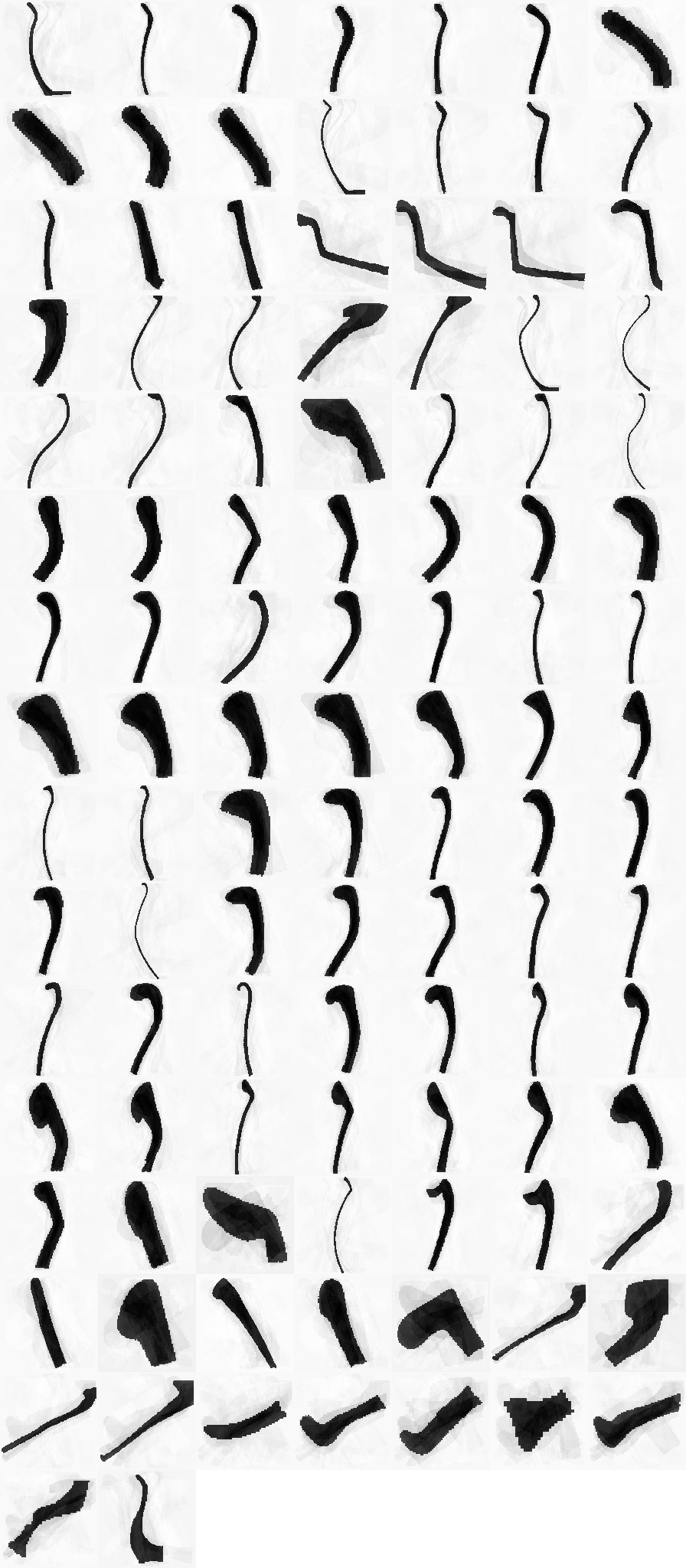
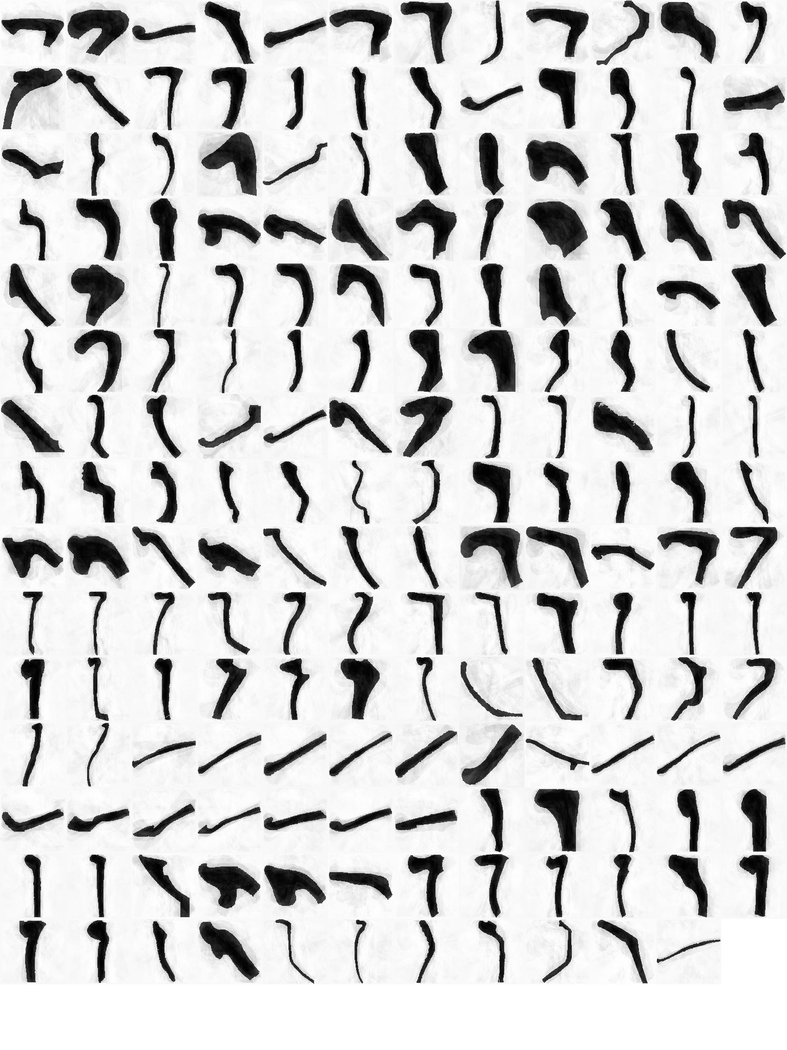
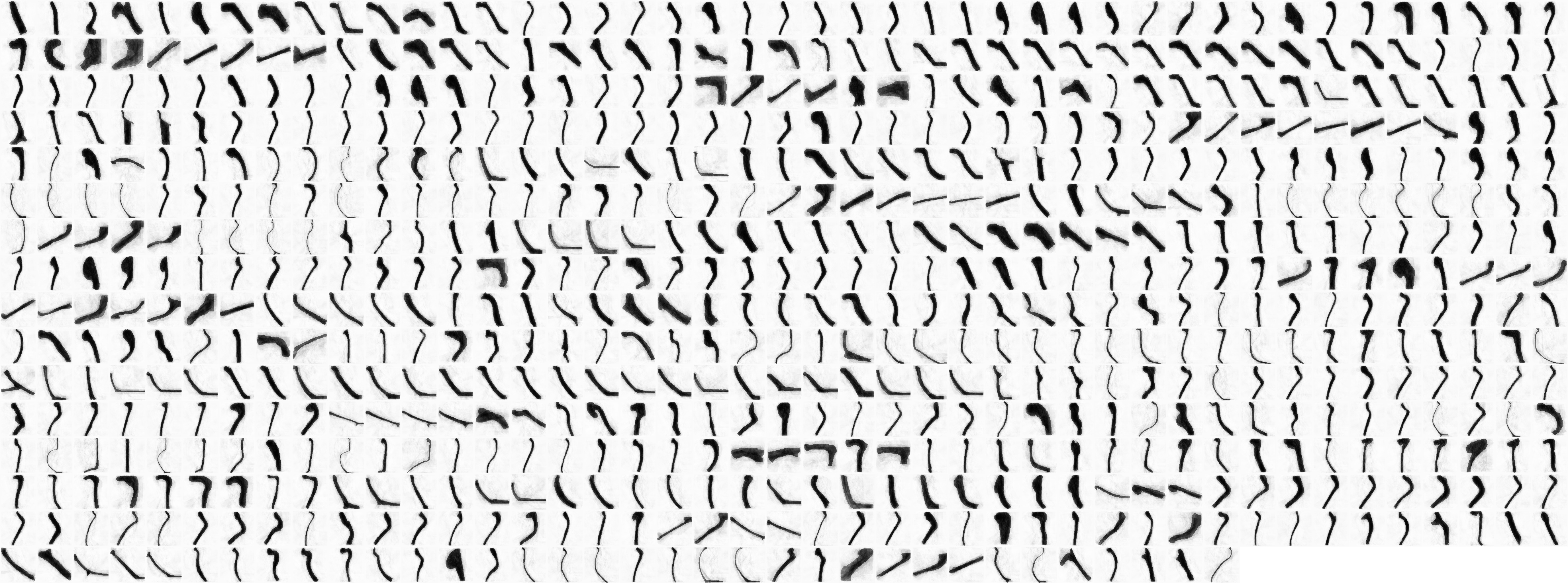
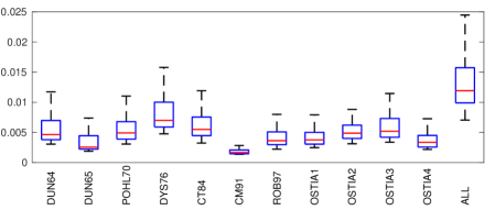
Our SSAE network in Figure 7 is composed by 3 stacked layers (each IDCAT experiment is trained with its number of profiles, see Table 1) for a maximum number of 500 epochs: the first layer has 625 neurons, the second 400 and the third 256. Each layer learns how to minimise the cost function in (5), with the logsig transfer function both in the encoder and decoder step and with $\lambda=0.004$ and $\beta=4$ and with 15% of training examples a neuron reacts to. At the end of the training, we are able to reconstruct in Figure 7 the original profiles of Figure 4 by means of 256 features, which can now be used in the hierarchical clustering step. We report in Figure 7 the confidence intervals of the mean squared reconstruction error: the positive skewness of the boxplots indicates that the frequencies of low errors in the reconstruction occour more often than than large errors. Both visual and quantitative results confirms that the shapes are reconstructed almost correctly, meaning that the neurons in the latent space are now specialised in the reconstruction of the shapes seen in the database.

(a) SAE (Layer 1)

(b) SAE (Layer 2)

(c) SAE (Layer 3)

(d) Network of the Stacked Sparse Auto-Encoder (SSAE) used in our strategy.

Figure 5: Representation of the single layers (first row) for the stacked network (second row) of sparse autoencoders for learning the shape features on profiles in Figure 4.

(e) DUN64

(f) DUN65

(g) POHL70

(h) DYS76

(i) CT84

(j) CM91

(k) ROB97

(l) OSTIA1

(m) OSTIA2

(n) OSTIA3

(o) OSTIA4

Figure 6: Reconstruction of Figure 4 with the SSAE network in Figure 7.

Figure 7: Confidence of the Mean Squared Reconstruction Error for each experiment.

4.0.1 Hierarchical clustering.

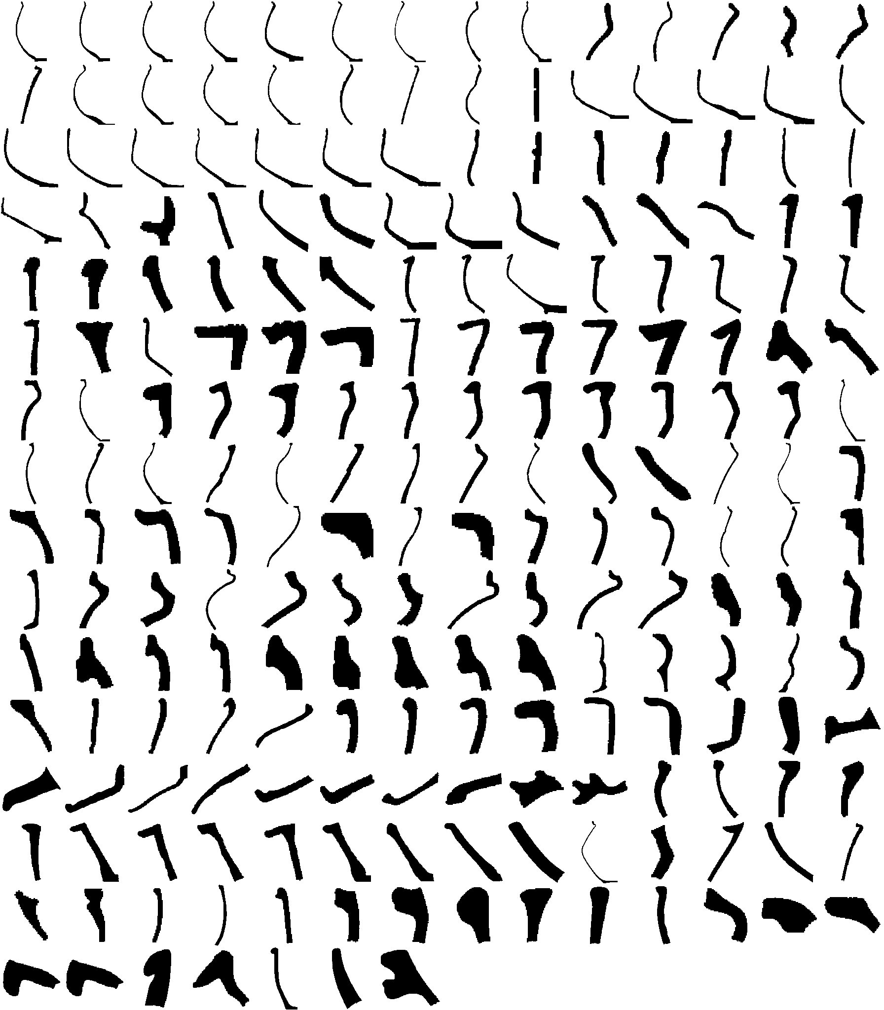
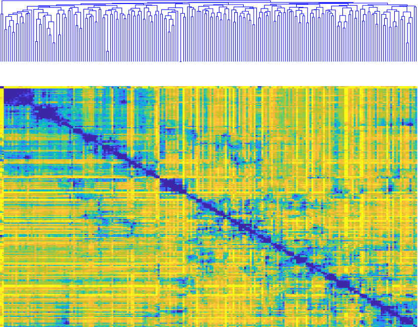
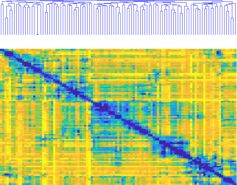
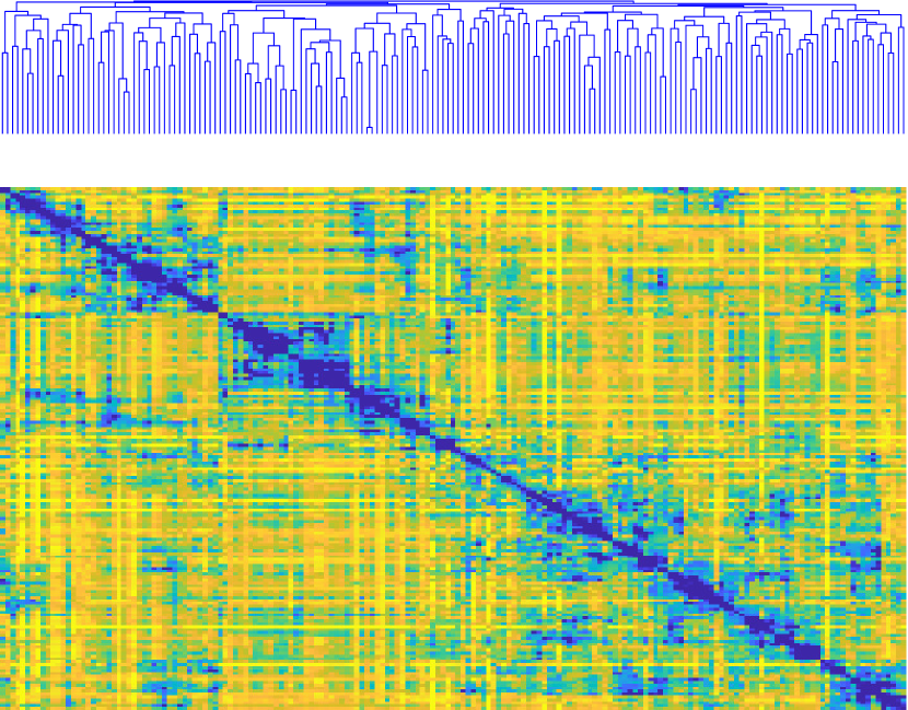
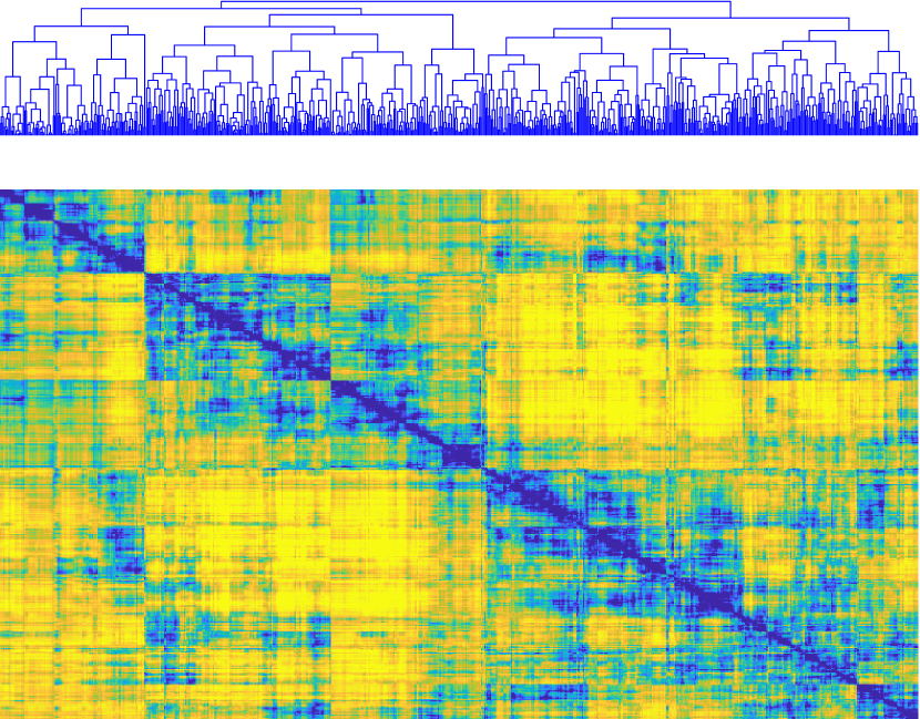
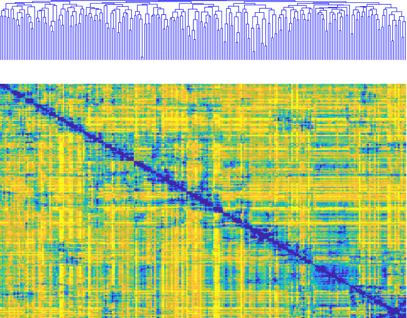
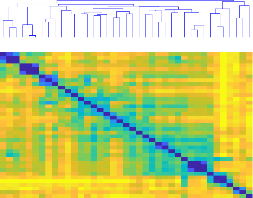
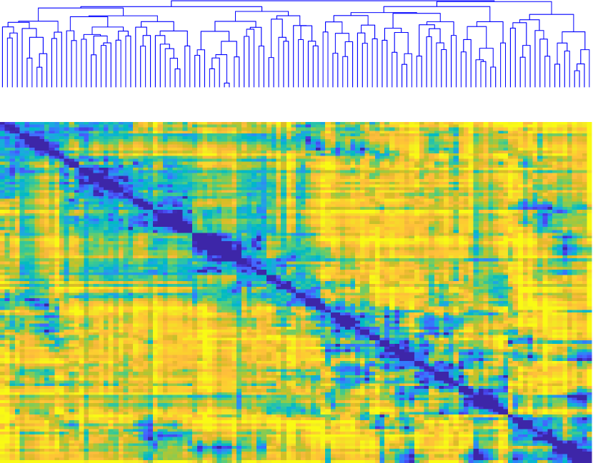
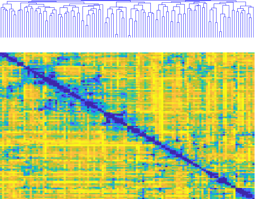
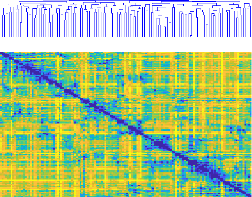
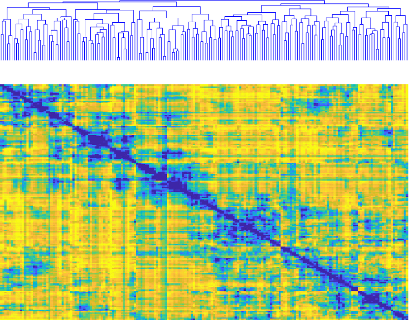
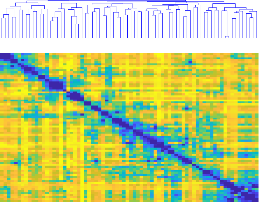
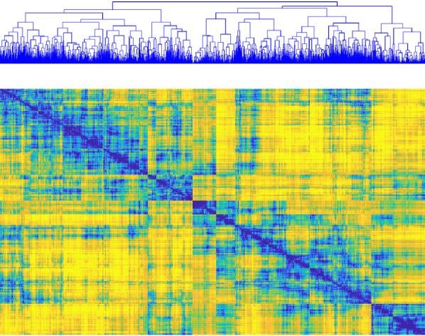
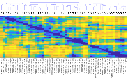
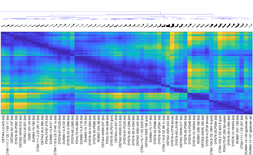
As said, our key idea is to take advantage of the learned features with SSAE for the hierarchical clustering task. For each experiment, we selected the hierarchical clustering with method and metric among the ones in Table 2, associated to the highest cophenet coefficient: selected choices and values are reported in Table 3, as well as the total number of rims under consideration, the total number of classes obtained and the coherency analysis performed by specialist archaeologists on the so-called seeds, i.e. the classes with exactly two shapes at the bottom level of the dendrogram. In most of the cases we observed that best cophenet coefficient is associated to the method average with metric chebychev: such result is not totally unexpected as the average method indicates that all distances between objects from each pair of clusters contribute equally to the mean distance between the clusters while the chebychev metric is based on the maximum coordinate difference between features, effectively useful for a small database of very different rims. When the number of data increases, as in the experiments DYS79 and ALL, then the cosine metric is preferred, which is again not surprising since it is a widely used metric in data mining for measuring cohesion within clusters of data [55]. Final dendrograms for each experiment in Figure 8.

Unveiling the invisible profile relations.

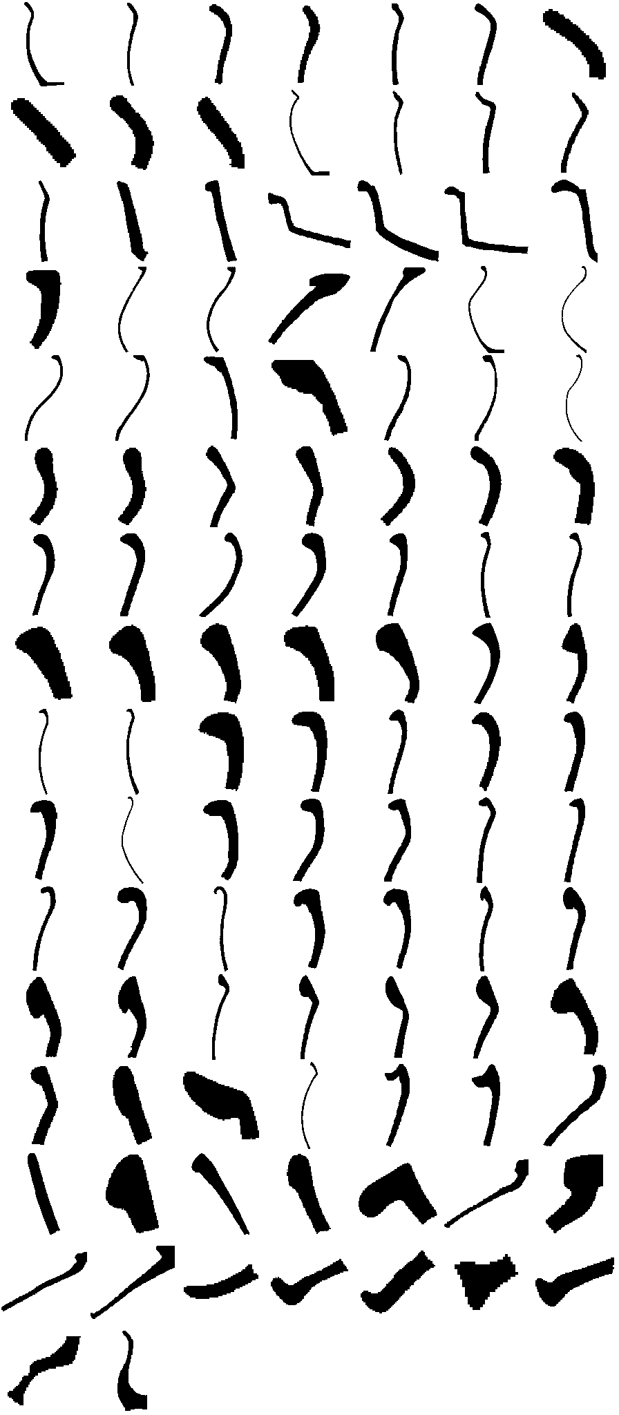
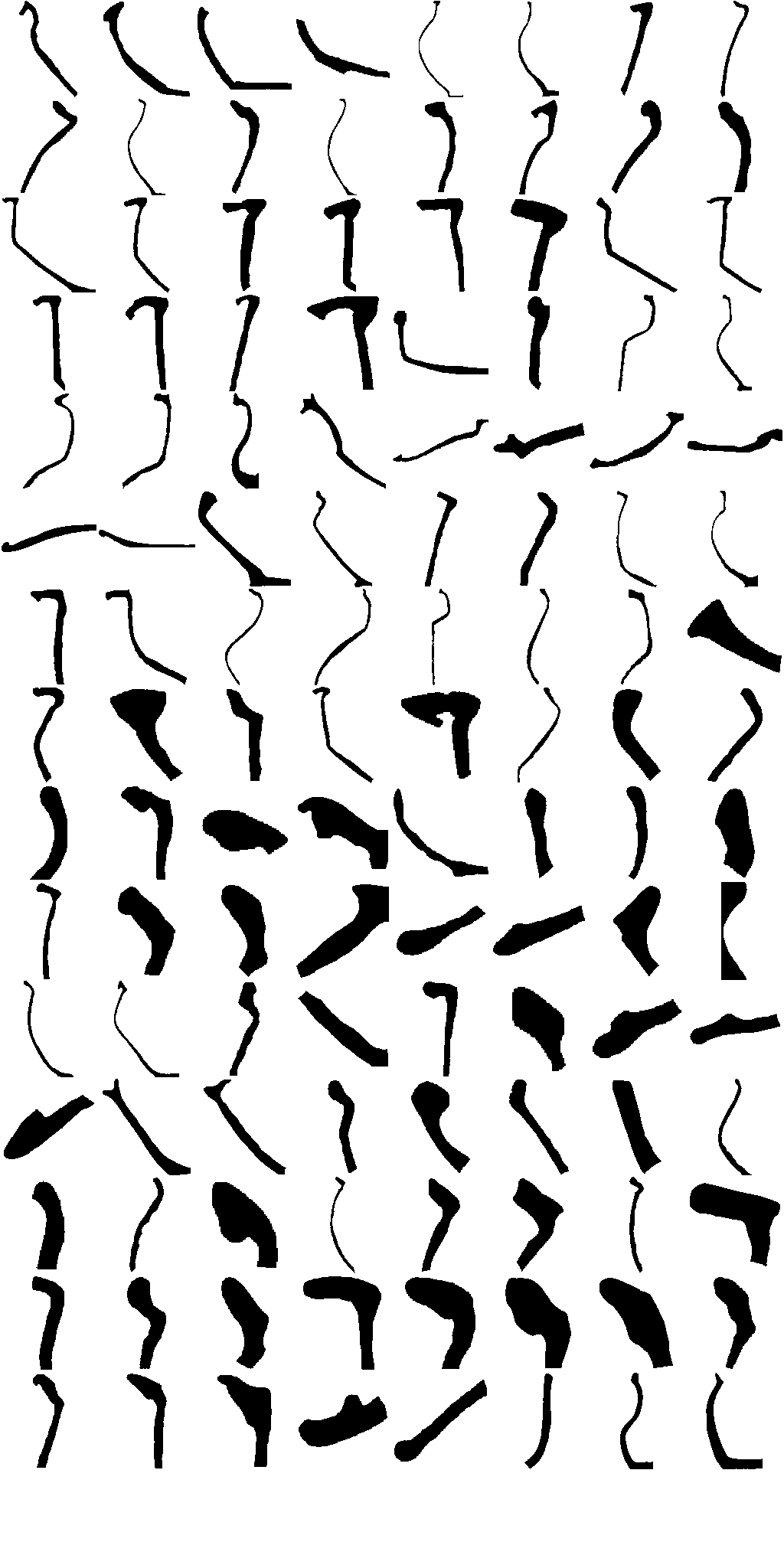
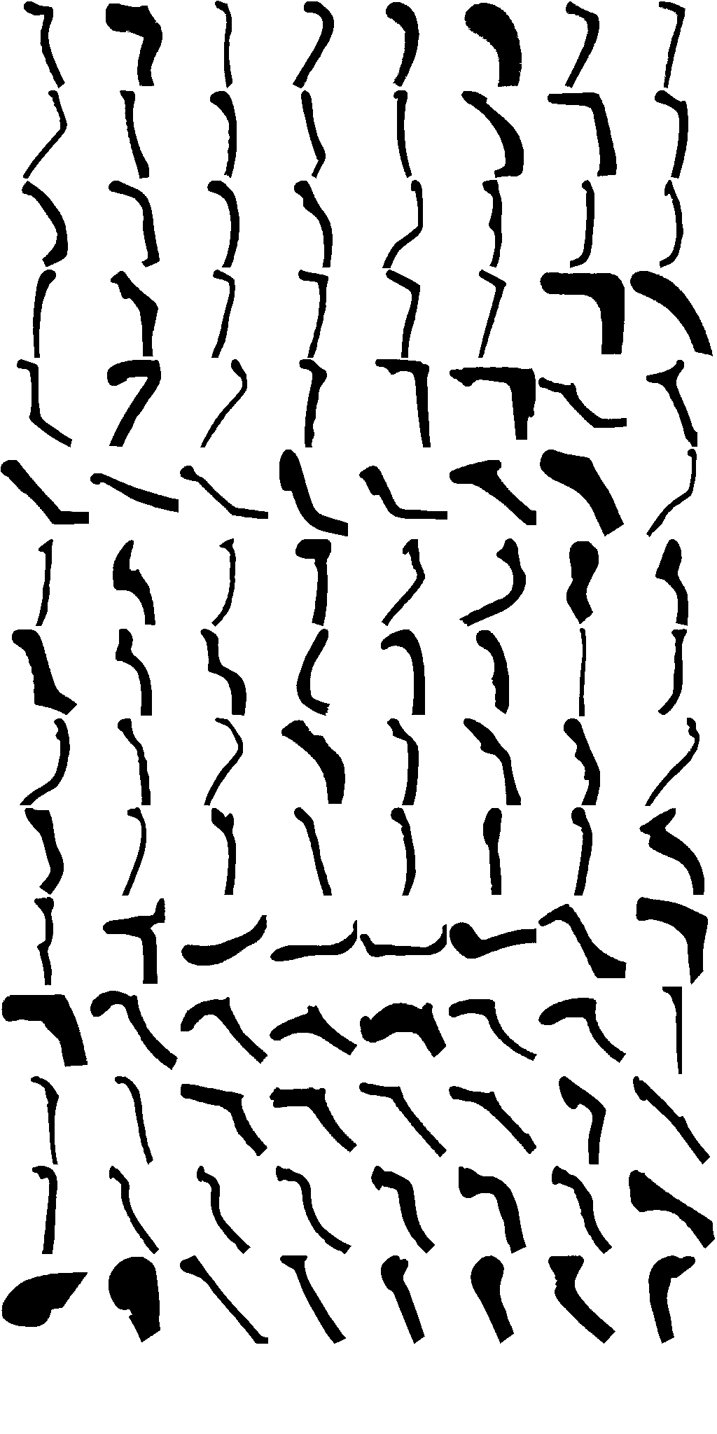
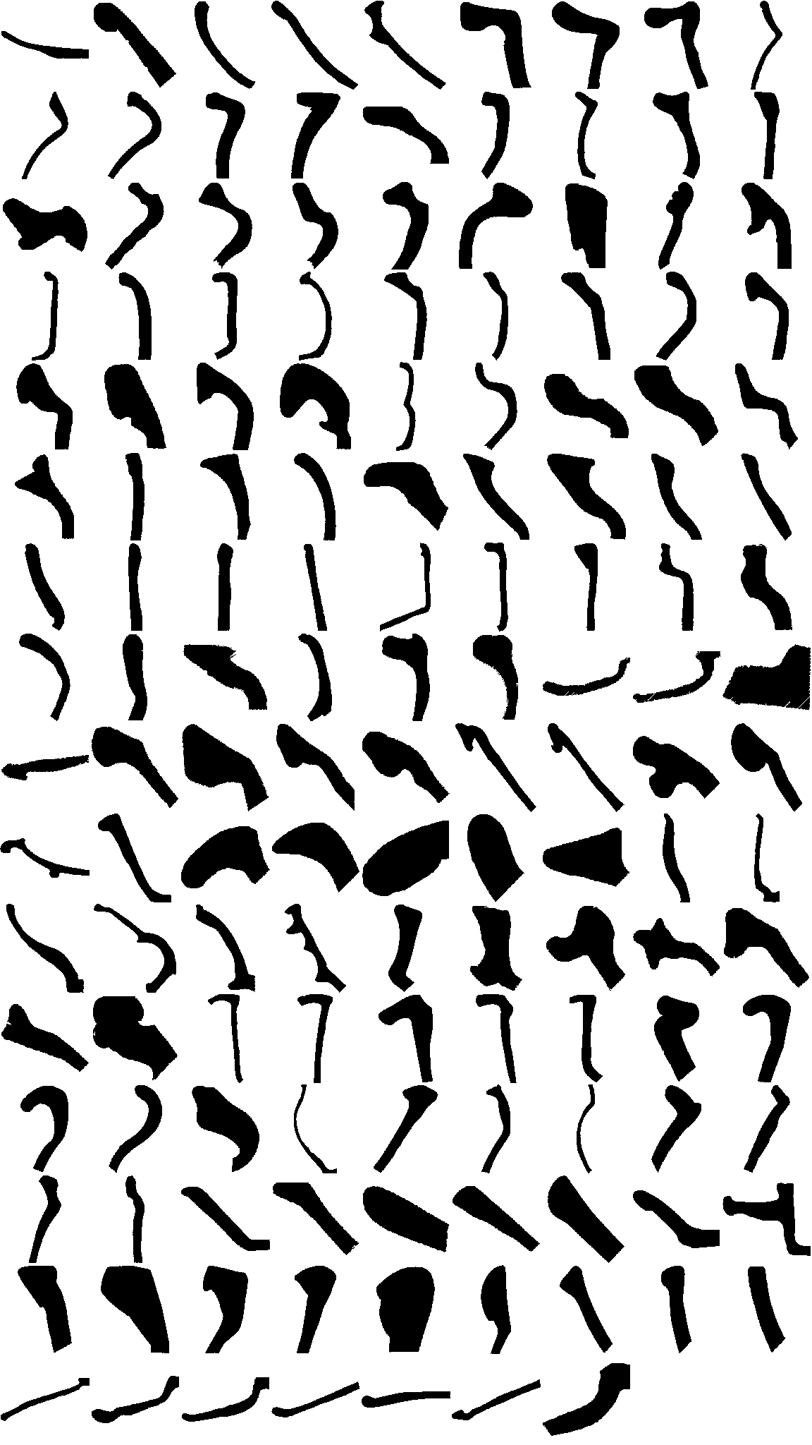
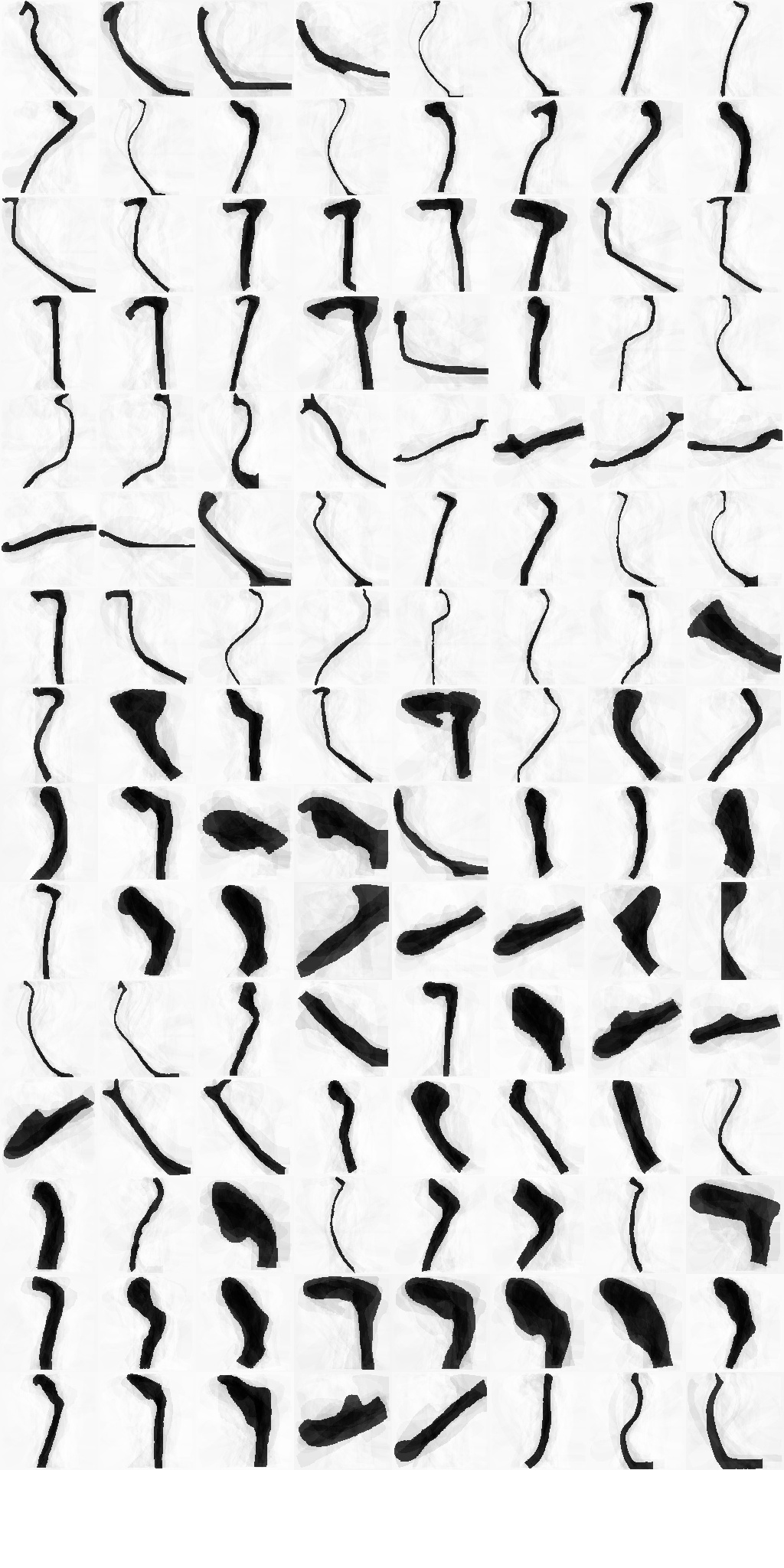
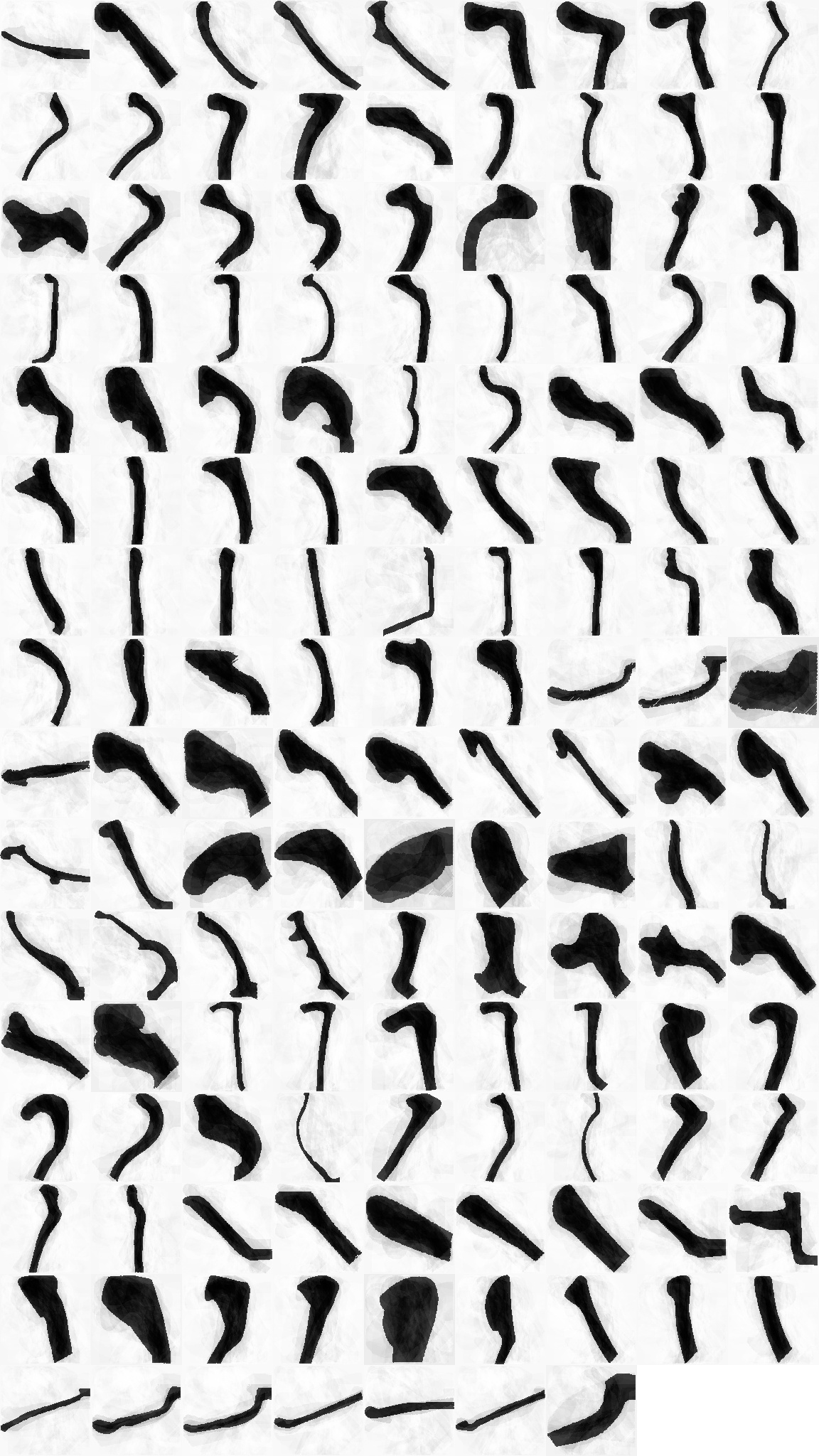
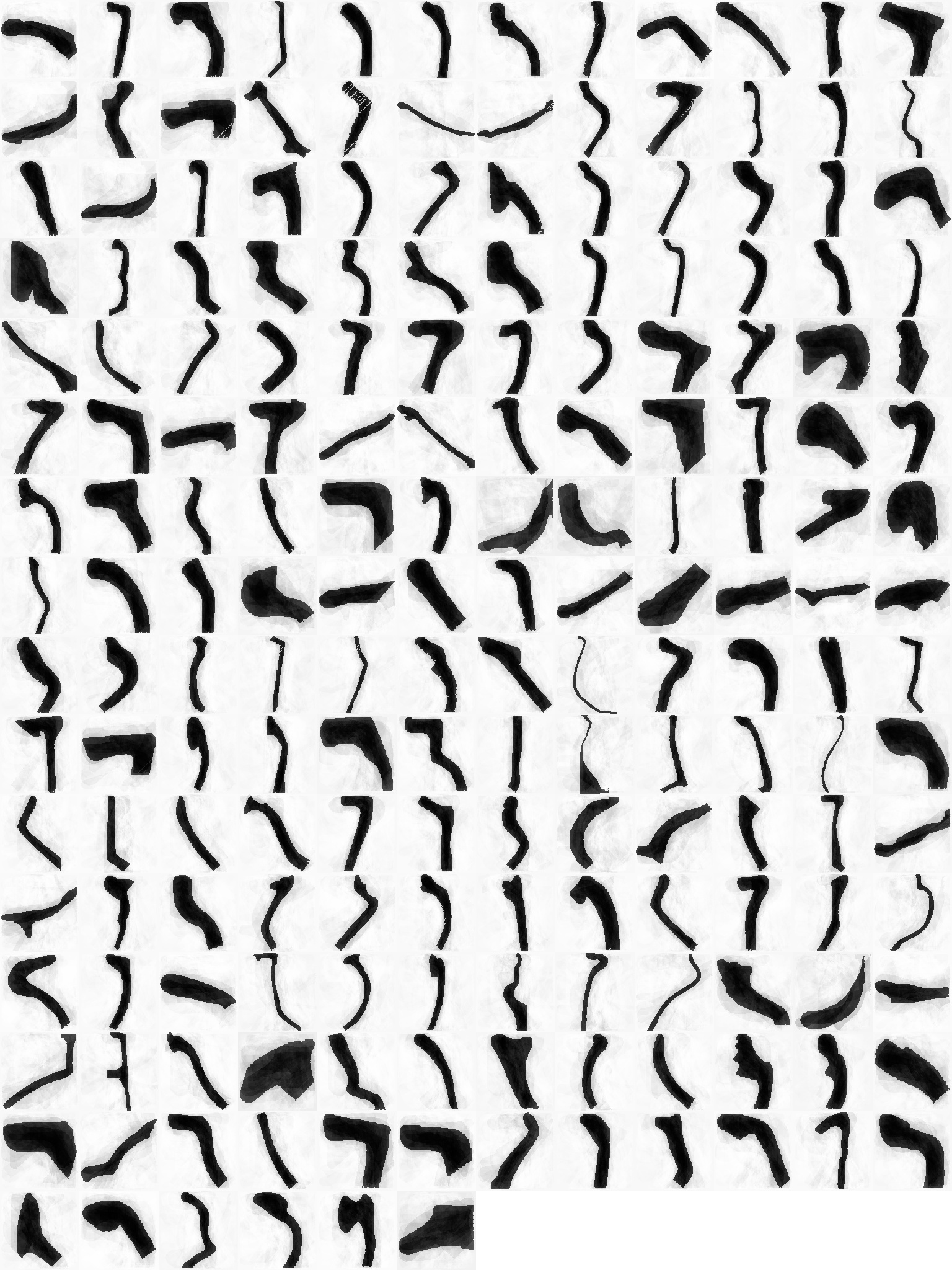
Given the cross-discipline nature of the collaboration described in this paper, we aim to explore possible shared research directions for data scientists and archaeologists. On top of the already established classification provided by the authors of each catalogue, we may be prompted to unveil new similarities between profiles, so as to hand in to experts an additional tool for the inspection of pottery catalogues. However, the lack of a commonly accepted “ground truth” in this type of data and their partiality has an impact on the final evaluation of the performances. Nevertheless, from a data scientist point of view, we can see in Figure 8 that the similarity matrix of each experiment very well reflects the dendrogram structure, where tiny blocks on the matrix diagonal appears due to comparable features. This is particularly clear on catalogues with less data, e.g. CM91 or ROB97, while some macro-blocks, i.e. subclusters of many shapes, are particularly evident in DYS76. These plots also reflects the fact of the high variance in a small amount of data and therefore only the so-called “seeds” (with few expansion steps towards the top of the dendrogram) can provide a reliable cluster of similar shapes as checked in the results summarised in Table 3. The pairing of seeds appears very promising in so far as the workflow was able to bring together similar profiles among coherent sub-datasets (e.g. dish-lids), see e.g. the zoom of dendrograms with pottery profiles in Figures 10 and 10. However, the inclusion of profiles derived from both intact and partial vessels introduces an element of confusion which the system could not effectively deal with yet (e.g. it compares a rim-fragment with an entire pot). For the effectiveness of our approach in supporting the classification of the database, it will be necessary to identify vessel parts (rim, wall, base) in each profile and introduce this level of information in the proposed dataset ROCOPOT: this is left for future work.

Table 3: Details of results on Rims.

IDCAT	Rims	method	metric	cophenet	Classes	Coherency: #/Seeds (%)
						Positive		Negative
DUN64	217	average	chebychev	0.7217	216	61/79	(77%)	18/79	(13%)
DUN65	107	average	chebychev	0.7699	106	30/37	(81%)	07/37	(19%)
POHL70	179	average	chebychev	0.7081	178	35/65	(54%)	30/65	(46%)
DYS76	679	average	cosine	0.6854	678	184/234	(79%)	50/234	(21%)
CT84	240	average	chebychev	0.6633	239	59/82	(72%)	23/82	(28%)
CM91	39	weighted	chebychev	0.8129	38	12/14	(86%)	02/14	(14%)
ROB97	120	average	euclidean	0.7100	119	39/45	(87%)	06/45	(13%)
OSTIA1	120	average	chebychev	0.7173	119	36/44	(82%)	08/44	(18%)
OSTIA2	142	average	chebychev	0.6727	141	30/49	(61%)	19/49	(39%)
OSTIA3	186	average	euclidean	0.6517	185	31/67	(46%)	36/67	(54%)
OSTIA4	74	average	chebychev	0.7470	73	14/26	(53%)	12/26	(46%)
ALL	2103	average	cosine	0.6581	2102	463/742	(62%)	279/742	(38%)
Overall:	-	-	-	-	4194	985/1484	(66%)	499/1484	(34%)

(a) DUN64

(b) DUN65

(c) POHL70

(d) DYS76

(e) CT84

(f) CM91

(g) ROB97

(h) OSTIA1

(i) OSTIA2

(j) OSTIA3

(k) OSTIA4

(l) ALL

Figure 8: Dendrograms (top) reflecting the similarity matrix of features (bottom). Colors for similarity matrix are clipped to 3 and 97 percentile of data.

Figure 9: Zoom on the right-bottom of the similarity matrix in Fig. 8(g) (ROB97), associated dendrogram and shapes: similarity is unveiled also by metadata, e.g. proximity of types (like pots, jars and bowls) and string-name of profiles.

Figure 10: Zoom on the right-bottom of the similarity matrix in Fig. 8(l) (ALL), associated dendrogram and shapes: almost all profiles are recognised as lids from different corpora.

5 Conclusions and Future Works

In this paper, we provide evidence that the hierarchical clustering of shape features extracted from the latent subspace of stacked sparse autoencoders (SSAE) is an effective tool for exploring shape similarities for advanced applications in Cultural Heritage science. In particular, we applied this workflow on a newly-introduced database of ROman COmmonware POTtery profiles (ROCOPOT), supplying experts with additional comparison tools. The most obvious advantage provided by these tools rests in their ability to ease and speed up the processing of a very large number of profiles from different pottery catalogues within a coherent and unified analytical environment. In principle, this could be achieved by pre-sorting the dataset in the way described, presenting the pottery specialist with a selection of most likely matches, thus providing invaluable pointers in the development of a comprehensive typology of Roman commonware. However, this is yet to be achieved, as the complex and partial nature of the profiles makes the clustering problem very significant, especially for big shape variance and the lack of a commonly perceived ground truth. In the near future we envisage two research directions: firstly, we plan to increase the number of profiles available in our database to nearly 5000 objects; secondly, with the help of continuous feedback from specialists, we will focus on meaningful subregions of interest so as to explore if the relevancy of the rim can improve the results of the proposed approach. We expect to not only distinguish between lids and pans, but to unveil more patterns within each single category.

Acknowledgements.

The authors acknowledge the support from the Leverhulme Trust Research Project Grant (RPG-2018-121) “Unveiling the Invisible - Mathematics for Conservation in Arts and Humanities”. CBS further acknowledges support from the RISE projects CHiPS and NoMADS, the Cantab Capital Institute for the Mathematics of Information and the Alan Turing Institute.

References

- [1] Anselmino, L.: Ostia IV : le terme del nuotatore, scavo dell’ambiente XVI e dell’area XXV. Studi miscellanei ; 23, De Luca, Roma (1977)
- [2] ArchAIDE Consortium: ARCHAIDE portal for publications and outputs (2019). https://doi.org/10.5284/1050896
- [3] Banterle, F., Dellepiane, M., Evans, T., Gattiglia, G., Itkin, B., Zallocco, M.: The ArchAIDE project: Results and perspectives after the first year. In: Proceedings of the Eurographics Workshop on Graphics and Cultural Heritage. p. 161–164. GCH ’17, Eurographics Association, Goslar, DEU (2017). https://doi.org/10.2312/gch.20171308, https://doi.org/10.2312/gch.20171308
- [4] Bar, Y., Levy, N., Wolf, L.: Classification of artistic styles using binarized features derived from a deep neural network. In: Agapito, L., Bronstein, M.M., Rother, C. (eds.) Computer Vision - ECCV 2014 Workshops. pp. 71–84. Springer International Publishing, Cham (2015)
- [5] Berti, F.: Ostia II : le terme del nuotatore, scavo dell’ambiente I. Studi miscellanei (Seminario di archeologia e storia dell’arte greca e romana dell’Università di Roma); 16, De Luca, Roma (1970)
- [6] Bronstein, A.M., Bronstein, M.M., Bruckstein, A.M., Kimmel, R.: Analysis of two-dimensional non-rigid shapes. International Journal of Computer Vision 78(1), 67–88 (Sep 2007). https://doi.org/10.1007/s11263-007-0078-4
- [7] Bronstein, A.M., Bronstein, M.M., Kimmel, R.: Numerical Geometry of Non-Rigid Shapes. Springer New York (2009). https://doi.org/10.1007/978-0-387-73301-2
- [8] Cao, F., Lisani, J.L., Morel, J.M., Musé, P., Sur, F.: A Theory of Shape Identification. Springer Berlin Heidelberg (2008). https://doi.org/10.1007/978-3-540-68481-7
- [9] Carandini, A.: Ostia I: le terme del nuotatore, scavo dell’ambiente IV. Studi miscellanei; 13, De Luca, Roma (1968)
- [10] Carandini, A., Panella, C.: Ostia III: le terme del nuotatore. Scavo degli ambienti III, VI, VII. Scavo dell’ambiente V e di un saggio nell’area Sud-Ovest. Studi miscellanea ; 21, De Luca, Roma (1973)
- [11] Carbonara, A., Messineo, G.: Ceramica dalle fornaci della celsa. In: La Via Flaminia: da Porta del Popolo a Malborghetto, pp. 185–199. Studi e materiali dei musei e monumenti comunali di Roma, Quasar, Roma (1991)
- [12] Chiaramonte Treré, C.: Ceramica grezza e depurata (M). In: Bonghi Jovino, M. (ed.) Ricerche a Pompei: l’Insula 5 della Regio VI dalle origini al 79 d.C. : I (Campagne di scavo 1976-1979). Bibliotheca archaeologica; 5, “L’Erma” di Bretschneider, Roma (1984)
- [13] Christmas, J., Pitts, M.: Classifying and visualising roman pottery using computer-scanned typologies. Internet Archaeology 50(50) (May 2018). https://doi.org/10.11141/ia.50.14
- [14] Cohen-Addad, V., Kanade, V., Mallmann-trenn, F., Mathieu, C.: Hierarchical clustering: Objective functions and algorithms. J. ACM 66(4) (Jun 2019). https://doi.org/10.1145/3321386
- [15] Crowley, E.J., Zisserman, A.: In search of art. In: Agapito, L., Bronstein, M.M., Rother, C. (eds.) Computer Vision - ECCV 2014 Workshops. pp. 54–70. Springer International Publishing, Cham (2015)
- [16] Cui, M., Femiani, J., Hu, J., Wonka, P., Razdan, A.: Curve matching for open 2d curves. Pattern Recognition Letters 30(1), 1 – 10 (2009). https://doi.org/doi.org/10.1016/j.patrec.2008.08.013
- [17] d’Amico, M., Frosini, P., Landi, C.: Using matching distance in size theory: A survey. International Journal of Imaging Systems and Technology 16(5), 154–161 (2006). https://doi.org/10.1002/ima.20076
- [18] Duda, R.O., Hart, P.E., Stork, D.G.: Pattern Classification (2nd Edition). Wiley-Interscience, USA (2000)
- [19] Duncan, G.C.: A Roman pottery near Sutri. Papers of the British School at Roma 32(1), 38–88 (1964). https://doi.org/10.1017/S0068246200007248
- [20] Duncan, G.C.: Roman republican pottery from the vicinity of sutri (sutrium). Papers of the British School at Rome 33, 134–176 (1965)
- [21] Dyson, S.L.: Cosa: The utilitarian pottery. Memoirs of the American Academy in Rome 33, 3–175 (1976), http://www.jstor.org/stable/4238670
- [22] Fiorucci, M., Khoroshiltseva, M., Pontil, M., Traviglia, A., Del Bue, A., James, S.: Machine learning for cultural heritage: A survey. Pattern Recognition Letters 133, 102 – 108 (2020). https://doi.org/10.1016/j.patrec.2020.02.017
- [23] Florek, K., Łukaszewicz, J., Perkal, J., Steinhaus, H., Zubrzycki, S.: Sur la liaison et la division des points d’un ensemble fini. Colloquium Mathematicum 2(3-4), 282–285 (1951)
- [24] Ginosar, S., Haas, D., Brown, T., Malik, J.: Detecting people in cubist art. In: Agapito, L., Bronstein, M.M., Rother, C. (eds.) Computer Vision - ECCV 2014 Workshops. pp. 101–116. Springer International Publishing, Cham (2015)
- [25] Gonthier, N., Gousseau, Y., Ladjal, S., Bonfait, O.: Weakly supervised object detection in artworks. In: Computer Vision – ECCV 2018 Workshops. pp. 692–709. Springer International Publishing (2018)
- [26] Gunia, P., Baher, A., Möller, H.: Ceramalex – ein datenbankprojekt zur erschließung hellenistischer und römischer fundkeramik aus ägypten. Kölner und Bonner Archaeologica 2, 253–261 (2012)
- [27] Hörr, C., Lindinger, E., Brunnett, G.: Machine learning based typology development in archaeology. J. Comput. Cult. Herit. 7(1) (Apr 2014). https://doi.org/10.1145/2533988
- [28] Jain, A.K., Dubes, R.C.: Algorithms for Clustering Data. Prentice-Hall, Inc., USA (1988)
- [29] Jr., J.H.W.: Hierarchical grouping to optimize an objective function. Journal of the American Statistical Association 58(301), 236–244 (1963). https://doi.org/10.1080/01621459.1963.10500845
- [30] Kampel, M., Sablatnig, R., Costa, E.: Classification of archaeological fragments using profile primitives. In: In Computer Vision, Computer Graphics and Photogrammetry — a Common Viewpoint, Proceedings of the 25th Workshop of the Austrian Association for Pattern Recognition ( ÖAGM. pp. 151–158 (2001)
- [31] Karasik, A., Smilansky, U.: Computerized morphological classification of ceramics. Journal of Archaeological Science 38(10), 2644 – 2657 (2011). https://doi.org/10.1016/j.jas.2011.05.023
- [32] Kim, W.Y., Kim, Y.S.: A region-based shape descriptor using zernike moments. Signal Processing: Image Communication 16(1), 95 – 102 (2000). https://doi.org/10.1016/S0923-5965(00)00019-9
- [33] Launaro, A., Leone, N.: A view from the margin? roman commonwares and patterns of distribution and consumption at interamna lirenas (lazio). Journal of Roman Archaeology 31, 323–338 (2018). https://doi.org/10.1017/S1047759418001356
- [34] LeCun, Y., Cortes, C., Burges, C.: MNIST handwritten digit database. ATT Labs [Online]. Available: http://yann.lecun.com/exdb/mnist 2 (2010)
- [35] Litany, O., Rodolá, E., Bronstein, A.M., Bronstein, M.M.: Fully spectral partial shape matching. Comput. Graph. Forum 36(2), 247–258 (May 2017). https://doi.org/10.1111/cgf.13123
- [36] Manay, S., Cremers, D., Byung-Woo Hong, Yezzi, A.J., Soatto, S.: Integral invariants for shape matching. IEEE Transactions on Pattern Analysis and Machine Intelligence 28(10), 1602–1618 (2006)
- [37] Milligan, G.W.: An examination of the effect of six types of error perturbation on fifteen clustering algorithms. Psychometrika 45(3), 325–342 (Sep 1980). https://doi.org/10.1007/bf02293907, https://doi.org/10.1007/bf02293907
- [38] Ming-Kuei Hu: Visual pattern recognition by moment invariants. IRE Transactions on Information Theory 8(2), 179–187 (1962)
- [39] Ng, A., et al.: Sparse autoencoder. CS294A Lecture notes 72, 1–19 (2011)
- [40] Olshausen, B.A., Field, D.J.: Sparse coding with an overcomplete basis set: A strategy employed by V1? Vision Research 37(23), 3311 – 3325 (1997). https://doi.org/10.1016/S0042-6989(97)00169-7
- [41] Orton, C., Hughes, M.: Pottery in Archaeology. Cambridge Manuals in Archaeology, Cambridge University Press, 2 edn. (2013). https://doi.org/10.1017/CBO9780511920066
- [42] Piccoli, C., Aparajeya, P., Papadopoulos, G.T., Bintliff, J., Leymarie, F.F., Bes, P., van der Enden, M., Poblome, J., Daras, P.: Towards the automatic classification of pottery sherds: two complementary approaches. Across Space and Time. Papers from the 41st Conference on Computer Applications and Quantitative Methods in Archaeology pp. 463–474 (2015)
- [43] Raviv, D., Bronstein, M.M., Bronstein, A.M., Kimmel, R.: Volumetric heat kernel signatures. In: Proceedings of the ACM Workshop on 3D Object Retrieval. p. 39–44. 3DOR ’10, Association for Computing Machinery, New York, NY, USA (2010). https://doi.org/10.1145/1877808.1877817
- [44] Roberts, P.: The roman pottery. In: Potter, T.W. (ed.) Excavations at the Mola di Monte Gelato: a Roman and Medieval settlement in south Etruria. Archaeological monographs of the British School at Rome; no.11, British School at Rome London in association with the British Museum, London (1997)
- [45] Rumpf, M., Wirth, B.: Discrete geodesic calculus in shape space and applications in the space of viscous fluidic objects. SIAM Journal on Imaging Sciences 6(4), 2581–2602 (2013). https://doi.org/10.1137/120870864
- [46] Seidl, M., Wieser, E., Zeppelzauer, M., Pinz, A., Breiteneder, C.: Graph-based shape similarity of petroglyphs. In: Agapito, L., Bronstein, M.M., Rother, C. (eds.) Computer Vision - ECCV 2014 Workshops. pp. 133–148. Springer International Publishing, Cham (2015)
- [47] Shen, W., Wang, Y., Bai, X., Wang, H., Latecki], L.J.: Shape clustering: Common structure discovery. Pattern Recognition 46(2), 539 – 550 (2013). https://doi.org/10.1016/j.patcog.2012.07.023
- [48] Shilane, P., Min, P., Kazhdan, M., Funkhouser, T.: The Princeton shape benchmark. In: Shape Modeling International (Jun 2004)
- [49] Smith, N.G., Karasik, A., Narayanan, T., Olson, E.S., Smilansky, U., Levy, T.E.: The pottery informatics query database: A new method for mathematic and quantitative analyses of large regional ceramic datasets. Journal of Archaeological Method and Theory 21(1), 212–250 (Sep 2012). https://doi.org/10.1007/s10816-012-9148-1
- [50] Sokal, R.R., Michener, C.D.: A statistical method for evaluating systematic relationships. University of Kansas Science Bulletin 38, 1409–1438 (1958)
- [51] Sokal, R.R., Rohlf, F.J.: The comparison of dendrograms by objective methods. TAXON 11(2), 33–40 (1962). https://doi.org/10.2307/1217208
- [52] Sørensen, T.: A Method of Establishing Groups of Equal Amplitude in Plant Sociology Based on Similarity of Species Content and Its Application to Analyses of the Vegetation on Danish Commons. Biologiske skrifter, I kommission hos E. Munksgaard (1948)
- [53] Sun, J., Ovsjanikov, M., Guibas, L.: A concise and provably informative multi-scale signature based on heat diffusion. In: Proceedings of the Symposium on Geometry Processing. p. 1383–1392. SGP ’09, Eurographics Association, Goslar, DEU (2009)
- [54] Sun, K.B., Super, B.J.: Classification of contour shapes using class segment sets. In: 2005 IEEE Computer Society Conference on Computer Vision and Pattern Recognition (CVPR’05). vol. 2, pp. 727–733 vol. 2 (2005)
- [55] Tan, P.N., Steinbach, M., Kumar, V.: Introduction to data mining. Pearson Education India (2016)
- [56] Tyers, P.A.: Roman Pottery in Britain. B. T. Batsford, London (1996), reprinted by Routledge in 1999 and 2003 with ISBN 0-415-21441-6
- [57] University Of Southampton: Roman Amphorae: a digital resource (2014). https://doi.org/10.5284/1028192
- [58] Veksler, O.: Cs 434a/541a pattern recognition (Fall 2004), https://www.csd.uwo.ca/~oveksler/Courses/CS434a_541a/outline.html
- [59] Vincent, P., Larochelle, H., Lajoie, I., Bengio, Y., Manzagol, P.A.: Stacked denoising autoencoders: Learning useful representations in a deep network with a local denoising criterion. J. Mach. Learn. Res. 11, 3371–3408 (Dec 2010)
- [60] Xu, J., Xiang, L., Liu, Q., Gilmore, H., Wu, J., Tang, J., Madabhushi, A.: Stacked sparse autoencoder (SSAE) for nuclei detection on breast cancer histopathology images. IEEE Transactions on Medical Imaging 35(1), 119–130 (Jan 2016). https://doi.org/10.1109/tmi.2015.2458702
- [61] Zevi, F., Pohl, I.: Ostia: saggi di scavo. Atti della Accademia Nazionale dei Lincei. Notizie degli scavi di antichità. Supplemento, Accademia nazionale dei Lincei, Roma (1970)
- [62] Zhu, Q., Wang, X., Keogh, E., Lee, S.H.: An efficient and effective similarity measure to enable data mining of petroglyphs. Data Mining and Knowledge Discovery 23(1), 91–127 (Sep 2010). https://doi.org/10.1007/s10618-010-0200-z, https://doi.org/10.1007/s10618-010-0200-z
- [63] Žunić, D., Žunić, J.: Shape ellipticity from hu moment invariants. Applied Mathematics and Computation 226, 406–414 (2014). https://doi.org/10.1016/j.amc.2013.10.062