Decomposable sparse polynomial systems

Abstract.

The Macaulay2 package DecomposableSparseSystems implements methods for studying and numerically solving decomposable sparse polynomial systems. We describe the structure of decomposable sparse systems and explain how the methods in this package may be used to exploit this structure, with examples.

1. Introduction

Améndola and Rodriguez [1] gave numerical methods to efficiently solve systems of sparse polynomial equations in a family, when that family is decomposable (Definition 1). A consequence of Esterov’s study of Galois groups of systems of sparse polynomial equations [6] is that for sparse systems, recognizing and computing a decomposition is algorithmic. Solving a decomposable sparse system reduces to solving two smaller sparse polynomial systems. In [4], we presented algorithms to detect and compute such decompositions, and a recursive algorithm exploiting decomposability for solving a decomposable sparse polynomial system using numerical homotopy continuation.

The Macaulay2 package DecomposableSparseSystems implements methods for decomposable sparse polynomial systems. These include methods to detect decomposability, to compute a decomposition, and a recursive procedure to compute numerical solutions to a given decomposable sparse system. Detection and computation of decompositions uses integer linear algebra, including computing a Smith normal form and the corresponding monomial changes of variables. Numerical homotopy continuation is used to compute solutions. When no further decompositions are possible, the algorithm solves multivariate systems using numerical software chosen by the user (default: PHCPACK [9]), and solves univariate polynomials using companion matrices.

Using the methods in DecomposableSparseSystems to solve a decomposable system allows for quicker solving and more accurate solution counts than calling other solvers. One reason is that after each decomposition, the child systems always involve either fewer variables, or polynomials of smaller degree. The cost of the methods in DecomposableSparseSystems is low as they rely only on linear algebra and numerical homotopy algorithms.

2. Decomposable Sparse Polynomial Systems

A branched cover is a dominant map $\pi\colon X\to Y$ of irreducible varieties $X$ and $Y$ of the same dimension. There is a number $d$ (the degree of $\pi$) and an open dense subset $V$ of $Y$ such that $\pi^{-1}(v)$ consists of $d$ points for $v\in V$. When $d>1$, the branched cover is nontrivial.

Definition 1.

A branched cover $\pi\colon X\to Y$ is decomposable if it is a composition of nontrivial branched covers. That is, if there is a dense open subset $U\subset Y$ and a variety $Z$ such that $\pi^{-1}(U)\to U$ factors as

$$\pi^{-1}(U)\ \longrightarrow\ Z\ \longrightarrow\ U\,,$$

with each map a nontrivial branched cover. $\diamond$

In general it is not easy to determine if a branched cover is decomposable, or even to compute a decomposition for a decomposable branched cover. (See [1, Section 5.4] and [4, Section 1.2] for examples and a discussion.)

An integer vector $\alpha\in\mathbb{Z}^{n}$ is the exponent of a (Laurent) monomial ${\color[rgb]{0,0.5,1}x^{\alpha}}:=x_{1}^{\alpha_{1}}\dotsb x_{n}^{\alpha_{n}}$. A (complex) linear combination of monomials $\sum c_{\alpha}x^{\alpha}$ is a (Laurent) polynomial. Monomials are multiplicative maps $(\mathbb{C}^{\times})^{n}\to\mathbb{C}^{\times}$ and polynomials are maps $(\mathbb{C}^{\times})^{n}\to\mathbb{C}$. For a finite set $\mathcal{A}\subset\mathbb{Z}^{n}$ of exponents, the set of all polynomials whose monomials have exponents contained in $\mathcal{A}$ (have support $\mathcal{A}$) forms the vector space $\mathbb{C}^{\mathcal{A}}$. Given a list ${\mathcal{A}_{\bullet}}=(\mathcal{A}_{1},\dotsc,\mathcal{A}_{n})$ of finite subsets of $\mathbb{Z}^{n}$, write $\mathbb{C}^{\mathcal{A}_{\bullet}}$ for the vector space $\mathbb{C}^{\mathcal{A}_{1}}\oplus\dotsb\oplus\mathbb{C}^{\mathcal{A}_{n}}$ of lists $F=(f_{1},\dotsc,f_{n})$ of polynomials with $f_{i}$ having support $\mathcal{A}_{i}$. Such a list $F\in\mathbb{C}^{\mathcal{A}_{\bullet}}$ is a function $F\colon(\mathbb{C}^{\times})^{n}\to\mathbb{C}^{n}$, and $F=0$ is a system of sparse polynomials with support ${\mathcal{A}_{\bullet}}$ whose solutions are $F^{-1}(0)$.

Example 2.

Let ${\mathcal{A}_{\bullet}}=(\mathcal{A}_{1},\mathcal{A}_{2})$ be the pair of supports in $\mathbb{Z}^{2}$ illustrated in Figure 1.

Figure 1. A pair of supports.

The corresponding vector spaces of polynomials are

$$\mathbb{C}^{\mathcal{A}_{1}} = \left\{a_{1}+a_{2}xy^{2}+a_{3}x^{2}y+a_{4}x^{3}y^{3}\mid a_{i}\in\mathbb{C}\right\}\,,$$

$$\mathbb{C}^{A_{2}} = \left\{b_{1}+b_{2}y^{3}+b_{3}xy^{2}+b_{4}x^{4}y^{2}\mid b_{j}\in\mathbb{C}\right\}\,,$$

and $\mathbb{C}^{\mathcal{A}_{\bullet}}$ is the space of systems of the form

$$F\ =\ \begin{pmatrix}a_{1}+a_{2}xy^{2}+a_{3}x^{2}y+a_{4}x^{3}y^{3}\\ b_{1}+b_{2}y^{3}+b_{3}xy^{2}+b_{4}x^{4}y^{2}\end{pmatrix}\,,\quad a_{i},b_{j}\ \in\ \mathbb{C}\,.$$

In DecomposableSparseSystems, the family $\mathbb{C}^{\mathcal{A}_{\bullet}}$ is encoded by a list of matrices whose column vectors are the exponent vectors of each polynomial. Given a system $F\in\mathbb{C}^{\mathcal{A}_{\bullet}}$, these data can be extracted from a given system via the Macaulay2 function exponents. $\diamond$

The Bernstein-Kushnirenko Theorem [2] provides a sharp upper bound on the number of solutions to a system of sparse polynomials. Denote the convex hull of a set $\mathcal{A}\subseteq\mathbb{R}^{n}$ by $\text{conv}(\mathcal{A})$. Given a list of supports ${\mathcal{A}_{\bullet}}=(\mathcal{A}_{1},\dotsc,\mathcal{A}_{n})$, let $\operatorname{{\rm MV}}({\mathcal{A}_{\bullet}})$ be the mixed volume of the list $(\text{conv}(\mathcal{A}_{1}),\dotsc,\text{conv}(\mathcal{A}_{n}))$.

Theorem 3 (Bernstein-Kushnirenko).

Let ${\mathcal{A}_{\bullet}}$ be a list of $n$ finite subsets of $\mathbb{Z}^{n}$. For $F\in\mathbb{C}^{\mathcal{A}_{\bullet}}$, the number of isolated solutions in $(\mathbb{C}^{\times})^{n}$ to the system $F=0$ is bounded above by $\operatorname{{\rm MV}}({\mathcal{A}_{\bullet}})$ and this bound is achieved for $F$ lying in a dense, open subset of $\mathbb{C}^{\mathcal{A}_{\bullet}}$.

Define ${\color[rgb]{0,0.5,1}X_{\mathcal{A}_{\bullet}}}\subset(\mathbb{C}^{\times})^{n}\times\mathbb{C}^{\mathcal{A}_{\bullet}}$ to be the set of pairs $(x,F)$ such that $F(x)=0$. For $F\in\mathbb{C}^{\mathcal{A}_{\bullet}}$, the fiber $\pi^{-1}(F)$ of the map $\pi\colon X_{\mathcal{A}_{\bullet}}\to\mathbb{C}^{\mathcal{A}_{\bullet}}$ consists of solutions to $F=0$. By the Bernstein-Kushnirenko Theorem the map $\pi$ has degree $\operatorname{{\rm MV}}({\mathcal{A}_{\bullet}})$. When $\operatorname{{\rm MV}}({\mathcal{A}_{\bullet}})\geq 1$, it is a branched cover. When the branched cover $\pi:X_{\mathcal{A}_{\bullet}}\to\mathbb{C}^{\mathcal{A}_{\bullet}}$ is decomposable, we say the sparse system $F\in\mathbb{C}^{\mathcal{A}_{\bullet}}$ is decomposable. Decomposability depends only on the support ${\mathcal{A}_{\bullet}}$ of a system.

There are two transparent ways for a sparse system to decompose.

Lacunary

A system $F\in\mathbb{C}^{\mathcal{A}_{\bullet}}$ is lacunary if there is a surjective monomial map $\Phi\colon(\mathbb{C}^{\times})^{n}\to(\mathbb{C}^{\times})^{n}$ such that $F=G\circ\Phi$ for some sparse polynomial system $G$. We require that $\Phi$ be nontrivial in that its kernel is not the identity subgroup. A lacunary system $F=G\circ\Phi=0$ can be solved by computing solutions, $z_{1},\dotsc,z_{d}$, to the system $G=0$ and then computing the fibres $\Phi^{-1}(z_{1}),\dotsc,\Phi^{-1}(z_{d})$. In appropriate coordinates, $\Phi$ is diagonal, and $\Phi^{-1}(z)$ is obtained by extracting roots of the components of $z$.

Example 4.

Consider the following system with support from Example 2.

$$F(x,y)\ =\ \begin{pmatrix}1-2xy^{2}+3x^{2}y-4x^{3}y^{3}\\ 2+3y^{3}+5xy^{2}+7x^{4}y^{2}\end{pmatrix}\ =\ \begin{pmatrix}0\\ 0\end{pmatrix}$$

It is lacunary as it is the composition of the following maps.

$$G(s,t)\ =\ \begin{pmatrix}1-2st^{2}+3st-4s^{2}t^{3}\\ 2+3st^{3}+5st^{2}+7s^{2}t^{2}\end{pmatrix}\,,\quad\Phi(x,y)\ =\ (x^{3},x^{-1}y)\,.$$

This can be detected via the methods in DecomposableSparseSystems.

i1 : R = CC[x,y];

i2 : F = {1-2*x*y^2+3*x^2*y-4*x^3*y^3,2+3*y^3+5*x*y^2+7*x^4*y^2};

i3 : isLacunary F
o3 = true

The method isLacunary extracts the set of supports of the system and computes the Smith normal form of a matrix associated to these supports to determine whether the system is lacunary. $\diamond$

Triangular

A system $F\in\mathbb{C}^{\mathcal{A}_{\bullet}}$ is triangular if there exists $k<n$ so that after a monomial change of variables, the system $F$ has the form

$$F\ =\ (F_{1}(x_{1},\dotsc,x_{k}),\dotsc,F_{k}(x_{1},\dotsc,x_{k}),F_{k+1}(x_{1},\dotsc,x_{n}),\dotsc,F_{n}(x_{1},\dotsc,x_{n}))\,.$$

Solutions to triangular systems are computed by first computing the solutions $z_{1},\dotsc,z_{d}$ of the square subsystem $(F_{1},\dotsc,F_{k})=0$. A residual system is obtained by substituting $z_{1}$ into the original system for the first $k$ variables, $F_{2}(z_{1},x_{k+1},\dotsc,x_{n})$. Solutions to the original system are obtained by solving the residual system and then applying a homotopy algorithm as described in [4].

Example 5.

Consider the system

$$F(x,y,z)\ =\ \begin{pmatrix}y^{2}-2x+3x^{2}y\\ 2+3x^{2}y+5x^{4}y^{2}\end{pmatrix}\ =\ \begin{pmatrix}0\\ 0\end{pmatrix}\,.$$

Figure 2 shows the supports.

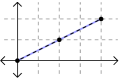
Figure 2. Triangular support.

This system is triangular as the second polynomial is quadratic in the monomial $x^{2}y$. The method isTriangular detects this subsystem.

i4 : F = {y^2-2*x+3*x^2*y,2+3*x^2*y+5*x^4*y^2};

i5 : isTriangular F
o5 = true

$\diamond$

A consequence of Esterov’s study of Galois groups of sparse polynomial systems [6] and Pirola and Schlesinger’s result that a branched cover is decomposable if and only if its Galois group is imprimitive [8] is that a sparse polynomial system is decomposable if and only if it is either lacunary or triangular. In each case, the solutions to original system are computed via solutions to simpler systems. The methods in DecomposableSparseSystems iteratively decompose these sparse polynomial systems to efficiently solve them.

3. Main method: solveDecomposableSystem

The main method implemented in the package DecomposableSparseSystems is named solveDecomposableSystem and this implements Algorithm 9 in [4]. It takes as input a sparse polynomial system $F\in\mathbb{C}^{{\mathcal{A}_{\bullet}}}$ and outputs all solutions to $F=0$ in the algebraic torus. It recursively checks whether or not the input sparse polynomial system is decomposable, computes the decomposition, and then calls itself on each portion of the decomposition. When the input is not decomposable it solves multivariate polynomial systems with the numerical solver given by the option Software (default: PHCPACK) and it solves univariate polynomial systems using companion matrices. For complete details see [4, Section 3.1].

3.1. Using the main method

Consider the system

$$F\ =\ \begin{pmatrix}2+xyz-x^{2}y\\ 4-y^{2}z+2xz^{2}-3x^{2}z\\ 1-yz^{2}-3xyz\end{pmatrix}\ =\ \begin{pmatrix}0\\ 0\\ 0\end{pmatrix}.$$

This system is supported on the triple ${\mathcal{A}_{\bullet}}=(\mathcal{A}_{1},\mathcal{A}_{2},\mathcal{A}_{3})$ shown in Figure 3.

Figure 3. Support of $F$.

The method isDecomposable determines that this system is decomposable. In particular, it is triangular with a subsystem indexed by the first and third polynomials. This can be observed in the figure as the span of the supports $\mathcal{A}_{1}$ and $\mathcal{A}_{3}$ are coplanar. It is also lacunary, as the exponent vectors lie in the sublattice of $\mathbb{Z}^{3}$ of index 3 generated by the columns of $\left(\begin{smallmatrix}1&1&2\\ 1&0&0\\ 1&2&1\end{smallmatrix}\right)$. The solutions to $F=0$ are found via the main method, solveDecomposableSystem.

i6 : R = CC[x,y,z];

i7 : F = {2+x*y*z-x^2*y,4-y^2*z+2*x*z^2-3*x^2*z,1-y*z^2-3*x*y*z};

  -- True if and only if the sparse system F is decomposable.
i8 : isDecomposable F
o8 : true

  -- A list of numerical solutions to F=0.
i9 : S = solveDecomposableSystem F;

  -- Evaluates F at the first numerical solution.
i10 : F/(f-> sub(f, matrix {S_0}))
o10 = {1.77636e-15, 4.44089e-16+1.4623e-16*ii, 4.66294e-15}

Our main method also accepts a two-argument input (A,C) where A is a list of matrices whose columns support a system of (Laurent) polynomial equations, and C is a list, whose $i$-th entry is the list of coefficients for the $i$-th polynomial equation. We demonstrate some of the other types of inputs here, and leave details to the documentation.

i11 : (A,C) = (F/exponents/matrix/transpose,
                F/coefficients/last/entries/flatten);

i12 : S = solveDecomposableSystem (A,C);

  -- Expected timing for solving a specific system.
i13 : benchmark "solveDecomposableSystem(A,C)";
o13 = .0605920270512821

  -- Expected timing for solving a random system with support A.
i14 : benchmark "solveDecomposableSystem(A, )";
o14 = .0558867168108108

3.2. Options for the main method

Numerical in nature, solveDecomposableSystem features a variety of options for the user. The option Software (default: PHCPACK) dictates which numerical solver is used to solve multivariate sparse systems which are not decomposable. The method solveDecomposableSystem removes solutions having any coordinate which is numerically zero up to Tolerance (default: $10^{-5}$) throughout the computation. Having this tolerance is necessary, as our methods are for Laurent polynomials with solutions in the complex torus $(\mathbb{C}^{\times})^{n}$, while the solvers we call may return solutions in $\mathbb{C}^{n}$ that are not in the torus.

When set to 1, the option Verify (default: 0) significantly increases the probability that solveDecomposableSystem computes the correct number of solutions.

It does this by checking that Software computes $\operatorname{{\rm MV}}({\mathcal{A}_{\bullet}})$ solutions to any system $F$ with support ${\mathcal{A}_{\bullet}}$, where $\operatorname{{\rm MV}}({\mathcal{A}_{\bullet}})$ is probabilistically determined using mixedVolume in the package Polyhedra [3]. If the mixed volume according to Polyhedra and the number of solutions do not agree, then the missing solutions are searched for using techniques related to those in MonodromySolver [5]. Lastly, we allow the user to compute the solutions to $F$ by first solving an internally generated random instance and then using that in a parameter homotopy [7] to solve $F$ by setting Strategy to FromGeneric. We conclude by using the options Verify and Strategy on an example with 6000 solutions.

i15 : A = <<< omitted, see example from Section 4 in [4] with
              i_1=(2,0,0,2,0)
              i_2=(4,4,2,2,2)
              j_1=(0,2,0,1,3)
              j_2=(0,0,1,0,2)
              >>;

  -- A has five supports, print the first one
i16 : print(length A,  A_0)
(5, | 0 2 4 4 6 |)
    | 0 0 0 4 4 |
    | 0 0 0 2 2 |
    | 0 2 4 2 4 |
    | 0 0 0 2 2 |

i17 : elapsedTime (F,S) = solveDecomposableSystem(A,,Verify=>1);
     -- 8.93938 seconds elapsed

i18 : elapsedTime S’ = solveDecomposableSystem(F,Strategy=>FromGeneric);
     -- 29.0802 seconds elapsed

i19 : print(#S,#S’)
o19 = (6000, 6000)

References

- [1] C. Améndola and J. I. Rodriguez. Solving parameterized polynomial systems with decomposable projections, 2016. arXiv:1612.08807.
- [2] D. N. Bernstein. The number of roots of a system of equations. Funkcional. Anal. i Priložen., 9(3):1–4, 1975.
- [3] R. Birkner. Polyhedra: a package for computations with convex polyhedral objects. J. Softw. Algebra Geom., 1:11–15, 2009.
- [4] T. Brysiewicz, J. I. Rodriguez, F. Sottile, and T. Yahl. Solving decomposable sparse systems, 2020. arXiv:2001.04228.
- [5] T. Duff, C. Hill, A. Jensen, K. Lee, A. Leykin, and J. Sommars. Solving polynomial systems via homotopy continuation and monodromy. IMA J. Numer. Anal., 39(3):1421–1446, 2019.
- [6] A. Esterov. Galois theory for general systems of polynomial equations. Compos. Math., 155(2):229–245, 2019.
- [7] T. Y. Li, T. Sauer, and J. A. Yorke. The cheater’s homotopy: an efficient procedure for solving systems of polynomial equations. SIAM J. Numer. Anal., 26(5):1241–1251, 1989.
- [8] G. P. Pirola and E. Schlesinger. Monodromy of projective curves. J. Algebraic Geom., 14(4):623–642, 2005.
- [9] J. Verschelde. Algorithm 795: PHCpack: A general-purpose solver for polynomial systems by homotopy continuation. ACM Trans. Math. Softw., 25(2):251–276, 1999. Available at http://www.math.uic.edu/~jan.