Path Sample-Analytic Gradient Estimators
for Stochastic Binary Networks

Abstract

In neural networks with binary activations and or binary weights the training by gradient descent is complicated as the model has piecewise constant response. We consider stochastic binary networks, obtained by adding noises in front of activations. The expected model response becomes a smooth function of parameters, its gradient is well defined but it is challenging to estimate it accurately. We propose a new method for this estimation problem combining sampling and analytic approximation steps. The method has a significantly reduced variance at the price of a small bias which gives a very practical tradeoff in comparison with existing unbiased and biased estimators. We further show that one extra linearization step leads to a deep straight-through estimator previously known only as an ad-hoc heuristic. We experimentally show higher accuracy in gradient estimation and demonstrate a more stable and better performing training in deep convolutional models with both proposed methods.

1 Introduction

Neural Networks with binary weights and binary activations are very computationally efficient. Rastegari et al. [24] report up to $58{\times}$ speed-up compared to floating point computations. There is a further increase of hardware support for binary operations: matrix multiplication instructions in recent NVIDIA cards, specialized projects on spike-like (neuromorphic) computation [3, 7], etc.

Binarized (or more generally quantized) networks have been shown to close up in performance to real-valued baselines [2, 22, 25, 29, 12, 6]. We believe that good training methods can improve their performance further. The main difficulty with binary networks is that unit outputs are computed using $\operatorname{sign}$ activations, which renders common gradient descent methods inapplicable. Nevertheless, experimentally oriented works ever so often define the lacking gradients in these models in a heuristic way. We consider the more sound approach of stochastic Binary Networks (SBNs) [19, 23]. This approach introduces injected noises in front of all $\operatorname{sign}$ activations. The network output becomes smooth in the expectation and its derivative is well-defined. Furthermore, injecting noises in all layers makes the network a deep latent variable model with a very flexible predictive distribution.

Estimating gradients in SBNs is the main problem that we address. We focus on handling deep dependencies through binary activations, which we believe to be the crux of the problem. That is why we consider all weights to be real-valued in the present work. An extension to binary weights would be relatively simple, e.g. by adding an extra stochastic binarization layer for them.

SBN Model

Let $x^{0}$ denote the input to the network (e.g. an image to recognize). We define a stochastic binary network (SBN) with $L$ layers with neuron outputs $X^{1\dots L}$ and injected noises $Z^{1\dots L}$ as follows (Fig. 1 left):

$$\textstyle X^{0}=x^{0};\ \ \ \ \ \textstyle X^{k}=\operatorname{sgn}(a^{k}(X^{k-1};\theta^{k})-Z^{k});\ \ \ \ \ \ F=f(X^{L};\theta^{L+1}).$$ (1)

The output $X^{k}$ of layer $k$ is a vector in $\mathbb{B}^{n}$, where we denote binary states $\mathbb{B}=\{-1,1\}$. The network input $x^{0}$ is assumed real-valued. The noise vectors $Z^{k}$ consist of $n$ independent variables with a known distribution (e.g., logistic). The network pre-activation functions $a^{k}(X^{k-1};\theta^{k})$ are assumed differentiable in parameters $\theta^{k}$ and will be typically modeled as affine maps (e.g., fully connected, convolution, concatenation, averaging, etc.). Partitioning the parameters $\theta$ by layers as above, incurs no loss of generality since they can in turn be defined as any differentiable mapping $\theta=\theta(\eta)$ and handled by standard backpropagation.

The network head function $f(x^{L};\theta^{L+1})$ denotes the remainder of the model not containing further binary dependencies. For classification problems we consider the softmax predictive probability model $p(y|x^{L};\theta^{L+1})=\operatorname{softmax}(a^{L+1}(x^{L};\theta^{L+1}))$, where the affine transform $a^{L+1}$ computes class scores from the last binary layer. The function $f(X^{L};\theta^{L+1})$ is defined as the cross-entropy of the predictive distribution $p(y|x^{L};\theta^{L+1})$ relative to the training label distribution $p^{*}(y|x^{0})$.

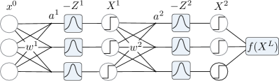
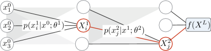
Figure 1: Stochastic binary network with 2 hidden layers. Left: latent variable model view (injected noises). Right: directed graphical model view (Bayesian network). The psa method performs explicit summation along paths (highlighted).

Due to the injected noises, all states $X$ become random variables and their joint distribution given the input $x^{0}$ takes the form of a Bayesian network with the following structure (Fig. 1 right):

$$\textstyle p(x^{1\dots L}\,|\,x^{0};\theta)=\prod_{k=1}^{L}p(x^{k}|x^{k-1};\theta^{k}),\ \ \ \ \ \ \textstyle p(x^{k}|x^{k-1};\theta^{k})=\prod_{i=1}^{n}p(x^{k}_{i}|x^{k-1};\theta^{k}).$$ (2a)

The equivalence to the injected noise model is established with

$$\textstyle p(x^{k}_{j}=1|x^{k-1};\theta^{k})=\mathbb{P}\big{(}a^{k}_{j}{-}Z^{k}_{j}>0\big{)}=F_{Z}(a^{k}_{j}),$$ (3)

where $F_{Z}$ is the noise cdf. If we consider noises with logistic distribution, $F_{Z}$ becomes the common sigmoid logistic function and the network with linear pre-activations $a^{k}(x^{k-1})_{j}=\sum_{j}w^{k}_{ij}x^{k-1}_{i}$ becomes the well-known sigmoid belief network [19].

Problem

The central problem for this work is to estimate the gradient of the expected loss:

$$\textstyle\frac{\partial}{\partial\theta}\mathbb{E}_{Z}[F(\theta)]=\frac{\partial}{\partial\theta}\sum_{x^{1\dots L}}p(x^{1\dots L}|x^{0};\theta)f(x^{L};\theta).$$ (4)

Observe that when the noise cdf $F_{Z}$ is smooth, the expected network output $\mathbb{E}_{Z}[F(\theta)]$ is differentiable in parameters despite having binary activations and a head function possibly non-differentiable in $x^{L}$. This can be easily seen from the Bayesian network form on the right of (4), where all functions are differentiable in $\theta$. The gradient estimation problem of this kind arises in several learning formulations, please see Appendix A for discussion.

Bias-Variance Tradeoff

A number of estimators for the gradient (4) exist, both biased and unbiased. Estimators using certain approximations and heuristics have been applied to deep SBNs with remarkable success. The use of approximations however introduces a systematic error, i.e. these estimators are biased. Many theoretical works therefore have focused on development of lower-variance unbiased stochastic estimators, but encounter serious limitations when applied to deep models. At the same time, allowing a small bias may lead to a considerable reduction in variance, and more reliable estimates overall. We advocate this approach and compare the methods using metrics that take into account both the bias and the variance, in particular the mean squared error of the estimator. When the learning has converged to 100% training accuracy (as we will test experimentally for the proposed method) the fact that we used a biased gradient estimator no longer matters.

Contribution

The proposed Path Sample-Analytic (psa) method is a biased stochastic estimator. It takes one sample from the model and then applies a series of derandomization and approximation steps. It efficiently approximates the expectation of the stochastic gradient by explicitly computing summations along multiple paths in the network Fig. 1 (right). Such explicit summation over many configurations gives a huge variance reduction, in particular for deep dependencies. The approximation steps needed for keeping the computation simple and tractable, are clearly understood linearizations. They are designed with the goal to obtain a method with the same complexity and structure as the usual backpropagation, including convolutional architectures. This allows to apply the method to deep models and to compute the gradients in parameters of all layers in a single backwards pass.

A second simplification of the method is obtained by further linearizations in psa and leads to the Straight-Through (ST) method. We thus provide the first theoretical justification of straight-through methods for deep models as derived in the SBN framework using a clearly understood linearization and partial summation along paths. This allows to eliminates guesswork and obscurity in the practical application of such estimators as well as opens possibilities for improving them. Both methods perform similar in learning of deep convolutional models, delivering a significantly more stable and better controlled training than preceding techniques.

1.1 Related Work

Unbiased estimators

A large class of unbiased estimators is based on the reinforce [34]. Methods developed to reduce its variance include learnable input-dependent [18] and linearization-based [10] control variates. Advanced variance reduction techniques have been proposed: rebar [33], relax [9], arm [35]. However the latter methods face difficulties when applied to deep belief models and indeed have never been applied to SBNs with more than two layers. One key difficulty is that they require $L$ passes through the network, leading to a quadratic complexity in the number of layers. We compare to arm, which makes a strong baseline according to comparisons in [35, 9, 33], in a small-problem setting. Previous direct comparison of estimator accuracy at the same point was limited to a single neuron setting [35], where psa would be simply exact. We also compare to MuProp [10] and variance-reduced reinforce, which run in linear time, in the deep setting in Section C.3. We observe that the variance of these estimators stays prohibitive for a practical application.

In the case of one hidden layer, our method coincides with several existing unbiased techniques [5, 31, 32]. The ram estimator [32] can be applied to deep models and stays unbiased but scales quadratically in the number of variables. Our estimator becomes biased for deep models but scales linearly.

Biased Estimators

Several works demonstrate successful training of deep networks using biased estimators. One such estimator, based on smoothing the $\operatorname{sign}$ function in the SBN model is the concrete relaxation [16, 13]. It has been successfully applied for training large-scale SBN in [22]. Methods that propagate moments analytically, known as assumed density filtering (ADF), e.g., [27, 8] perform the full analytic approximation of the expectation. ADF has been successfully used in [25].

Many experimentally oriented works successfully apply straight-through estimators (ste). Originally considered by Hinton [11] for deep auto-encoders with Bernoulli latent variables and by Bengio et al. [1] for conditional computation, these simple, but not theoretically justified methods were later adopted for training deterministic networks with binary weights and activations [6, 37, 12]. The method simply pretends that the $\operatorname{sign}$ function has the derivative of the identity, or of some other function. There have been recent attempts to justify why this works. Yin et al. [36] considers the expected loss over the training data distribution, which is assumed to be Gaussian, and show that in networks with 1 hidden layer the true expected gradient positively correlates with the deterministic ste gradient. Cheng et al. [4] show for networks with 1 hidden layer that ste is approximately related to the projected Wasserstein gradient flow method proposed there. In the case of one hidden layer Tokui & Sato [32, sec. 6.4] derived ste as a linearization of their ram estimator for SBN. We derive deep ste in the SBN model by making extra linearizations in our psa estimator.

2 Method

To get a proper view of the problem, we first explain the exact chain rule for the gradient, relating it to the reinforce and the proposed method. Throughout this section we will consider the input $x^{0}$ fixed and omit it from the conditioning such as in $p(x|x^{0})$.

2.1 Exact Chain Rule

The expected loss in the Bayesian network representation (2) can be written as

$$\textstyle\mathbb{E}_{Z}[F]=\textstyle\sum_{x^{1}\in\mathbb{B}^{n}}p(x^{1};\theta^{1})\sum_{x^{2}\in\mathbb{B}^{n}}p(x^{2}|x^{1};\theta^{2})\dots\sum_{x^{L}\in\mathbb{B}^{n}}p(x^{L}|x^{L-1};\theta^{L})f(x^{L};\theta^{L+1})$$ (5)

and can be related to the forward-backward marginalization algorithm for Markov chains. Indeed, let $P^{k}=p(x^{k}|x^{k-1};\theta^{k})$ be transition probability matrices of size $2^{n}{\times}2^{n}$ for $k>1$ and $P^{1}$ be a row vector of size $2^{n}$. Then (5) is simply the product of these matrices and the vector $f$ of size $2^{n}$. The computation of the gradient is as “easy”, e.g. for the gradient in $\theta^{1}$ we have:

$$g^{1}:=\textstyle\frac{\partial}{\partial\theta^{1}}\mathbb{E}_{Z}[F]= D^{1}P^{2}P^{3}\dots P^{L}f,$$ (6)

where $D^{1}$ is the size $\dim(\theta^{1}){\times}2^{n}$ transposed Jacobian $\frac{\partial p(x^{1};\theta^{1})}{\partial\theta^{1}}$. Expression (6) is a product of transposed Jacobians of a deep model. Multiplying them in the right-to-left order requires only matrix-vector products and it is the exact back-propagation algorithm. As impractical as it may be, it is still much more efficient than the brute force enumeration of all $2^{nL}$ joint configurations.

The well-known reinforce [34] method replaces the intractable summation over $x$ with sampling $x$ from $p(x^{1\dots L};\theta)$ and uses the stochastic estimate

$$\textstyle\frac{\partial}{\partial\theta^{1}}\mathbb{E}_{Z}[F]\approx\frac{\partial p(x^{1};\theta^{1})}{\partial\theta^{1}}\frac{f(x^{L})}{p^{1}(x^{1};\theta^{1})}.$$ (7)

While this is cheap to compute (and unbiased), it utilizes neither the shape of the function $f$ beyond its value at the sample nor the dependence structure of the model.

2.2 PSA Algorithm

We present our method for a deep model. The single layer case, is a special case which is well covered in the literature [32, 31, 5] and is discussed in Lemma B.1. Let us consider the gradient in parameters $\theta^{l}$ of layer $l$. Starting from the RHS of (4), we can move derivative under the sum and directly differentiate the product distribution (2):

$$g^{l}:=\textstyle\frac{\partial}{\partial\theta^{l}}\sum_{x}p(x;\theta)f(x^{L};\theta^{L+1})=\textstyle\sum_{x}f(x^{L})\frac{\partial}{\partial\theta^{l}}p(x;\theta)=\sum_{x}\frac{p(x)f(x^{L})}{p(x^{l}|x^{l-1})}\frac{\partial}{\partial\theta^{l}}p(x^{l}|x^{l-1};\theta^{l}),$$ (8)

where the dependence on $\theta$ in $p$ and $f$ is omitted once it is outside of the derivative. The fraction $\frac{p(x)}{p(x^{l}|x^{l-1})}$ is a convenient way to write the product $\prod_{k=1|k\neq l}^{L}p(k^{k}|x^{k-1})$, i.e. with factor $l$ excluded.

At this point expression (8) is the exact chain rule completely analogous to (6). A tractable back propagation approximation is obtained as follows. Since $p(x^{l}|x^{l-1};\theta^{l})=\prod_{i=1}^{n}p(x^{l}_{i}|x^{l-1};\theta^{l})$, its derivative in (8) results in a sum over units $i$:

$$g^{l}=\textstyle\sum_{x}\sum_{i}\frac{p(x)}{p(x^{l}_{i}|x^{l-1})}D^{l}_{i}(x)f(x^{L}),\ \ \ \ \ \ \ \text{where}\ \textstyle D^{l}_{i}(x)=\frac{\partial}{\partial\theta^{l}}p(x^{l}_{i}|x^{l-1};\theta^{l}).$$ (9)

We will apply a technique called derandomization or Rao-Blackwellization [20, ch. 8.7] to $x^{l}_{i}$ in each summand $i$. Put simply, we sum over the two states of $x^{l}_{i}$ explicitly. The summation computes a portion of the total expectation in a closed form and as such, naturally and guaranteed, reduces the variance. The estimator with this derandomization step is an instance of the general local expectation gradient [31]. The derandomization results in the occurrence of the differences of products:

$$\textstyle\prod_{j}p(x^{l+1}_{j}|x^{l}_{\downarrow i})-\textstyle\prod_{j}p(x^{l+1}_{j}|x^{l}),$$ (10)

where $x^{l}_{\downarrow i}$ denotes the state vector in layer $l$ with the sign of unit $i$ flipped. We approximate this difference of products by linearizing it (making a 1st order Taylor approximation) in the differences of its factor probabilities, i.e., replacing the difference (10) with

$$\textstyle\sum_{j}\prod_{j^{\prime}\neq j}p(x^{k+1}_{j^{\prime}}|x^{k})\Delta^{k+1}_{i,j}(x),\ \ \ \ \text{where }\Delta^{k+1}_{i,j}(x)=p(x^{k+1}_{j}{|}x^{k})-p(x^{k+1}_{j}{|}x^{k}_{\downarrow i}).$$ (11)

The approximation is sensible when $\Delta^{k+1}_{i,j}$ are small. This holds e.g., in the case when the model has many units in layer $k$ that all contribute to preactivation so that the effect of flipping a single $x^{k}_{i}$ is small.

Notice that the approximation results in a sum over units $j$ in the next layer $l{+}1$, which allows us to isolate a summand $j$ and derandomize $x^{l+1}_{j}$ in turn. Chaining these two steps, derandomization and linearization, from layer $l$ onward to the head function, we obtain summations over units in all layers $l\dots L$, equivalent to considering all paths in the network, and derandomize over all binary states along each such path (see Fig. 1 right). The resulting approximation of the gradient $g^{l}$ gives

$$\textstyle\tilde{g}^{l}=\sum_{x}p(x)D^{l}(x)\Delta^{l+1}(x)\cdots\Delta^{L}(x)df(x)=:\sum_{x}p(x)\hat{g}^{l}(x),$$ (12)

where $D^{l}$, defined in (9), is the Jacobian^T of layer probabilities in parameters (a matrix of size $\dim(\theta^{l}){\times}n$); $\Delta^{k}_{i,j}$ defined in (11) are $n{\times}n$ matrices, which we call discrete Jacobians^T; and $df$ is a column vector with coordinates $f(x^{L})-f(x^{L}_{\downarrow i})$, i.e. a discrete gradient of $f$. Thus a stochastic estimate $\hat{g}^{l}(x)$ is a product of Jacobians^T in the ordinary activation space and can therefore be conveniently computed by back-propagation, i.e. multiplying the factors in (12) from right to left.

This construction allows us to approximate a part of the chain rule for the Markov chain with $2^{n}$ states as a chain rule in a tractable space and to do the rest via sampling. This way we achieve a significant reduction in variance with a tractable computational effort. This computation effort is indeed optimal is the sense that it matches the complexity of the standard back-propagation, which matches the complexity of forward propagation alone, i.e., the cost of obtaining a sample $x\sim p(x)$.

Derivation

The formal construction is inductive on the layers. Consider the general case $l{<}L$. We start from the expression (9) and apply to it Proposition 1 below recurrently, starting with $J^{l}=D^{l}$. The matrices $J^{k}$ will have an interpretation of composite Jacobians^T from layer $l$ to layer $k$.

Proposition 1.

Let $J^{k}_{i}(x)$ be functions that depend only on $x^{1\dots k}$ and are odd in $x^{k}_{i}$: $J^{k}_{i}(x^{k})=-J^{k}_{i}(x^{k}_{\downarrow i})$ for all $i$. Then

$$\textstyle\sum_{x}p(x)\sum_{i}\frac{J^{k}_{i}(x)f(x^{L})}{p(x^{k}_{i}|x^{k-1})}\approx\textstyle\sum_{x}p(x)\sum_{j}\frac{J^{k+1}_{j}(x)f(x^{L})}{p(x^{k+1}_{j}|x^{k})},\ \ \ \ \text{where $J^{k+1}_{j}=\sum_{i}J^{k}_{i}(x)\Delta^{k+1}_{i,j}(x)$}$$ (13)

and the approximation made is the linearization (11). Functions $J^{k+1}_{j}$ are odd in $x^{k+1}_{j}$ for all $j$.

The structure of (13) shows that we will obtain an expression of the same form but with the dividing probability factor from the next layer, which allows to apply it inductively. To verify the assumptions at the induction basis, observe that according to (3), $\textstyle D^{l}_{i}(x)=\frac{\partial}{\partial\theta^{l}}p(x^{l}_{i}|x^{l-1};\theta^{l})=p_{Z}(a^{l}_{i})x^{l}_{i}\frac{\partial}{\partial\theta^{l}}a^{l}_{i}(x^{l-1};\theta^{l}),$ hence it depends only on $x^{l-1}$, $x^{l}$ and is odd in $x^{l}_{i}$.

In the last layer, the difference of head functions occurs instead of the difference of products. Thus instead of (13), we obtain for $k=L$ the expression

$$\textstyle\sum_{x}p(x)\sum_{i}\frac{J^{L}_{i}(x)f(x^{L})}{p(x^{L}_{i}|x^{L-1})}=\sum_{x}\sum_{i}p(x)J^{L}_{i}(x)df_{i}(x).$$ (14)

Applying Proposition 1 inductively, we see that the initial $J^{l}$ is multiplied with a discrete Jacobian^T $\Delta^{k+1}$ on each step $k$ and finally with $df$. Note that neither the matrices $\Delta^{k}$ nor $df$ depend on the layer we started from. The final result of inductive application of Proposition 1 is exactly the expected matrix product (12). The key for computing a one-sample estimate $\hat{g}(x)^{l}=D^{l}\Delta^{l+1}\cdots\Delta^{L}df$ is to perform the multiplication from right to left, which only requires matrix-vector products. Observe also that the part $\Delta^{k}\cdots\Delta^{L}df$ is common for our approximate derivatives in all layers $l<k$ and therefore needs to be evaluated only once.

Algorithm

Since backpropagation is now commonly automated, we opt to define forward propagation rules such that their automatic differentiation computes what we need. The algorithm in this form is presented in Algorithm 1. First, we have substituted the noise model (3) to compute $\Delta^{k}_{i,j}$ as in Algorithm 1. The detach method available in PyTorch [21] obtains the value of the tensor but excludes it from back-propagation. It is applied to $\Delta^{k}$ since it is already the Jacobian^T and we do not want to differentiate it. The recurrent computation of $q^{k}$ in Algorithm 1 serves to generate the computation of $\hat{g}^{l}(x)$ on the backward pass. Indeed, variables $q^{k}$ always store just zero values as ensured by Algorithm 1 but have non-zero Jacobians as needed. A similar construct is applied for the final layer. It is easy to see that differentiating the output $E$ w.r.t. $\theta^{l}$ recovers exactly $\hat{g}(x)^{l}=D^{l}\Delta^{l+1}\cdots\Delta^{L}df$.

This form is simpler to present and can serve as a reference. The large-scale implementation detailed in Section B.5 defines custom backward operations, avoiding the overhead of computing variables $q^{k}$ in the forward pass. The overhead however is a constant factor and the following claim applies.

Input: Network parameters $\theta$, input $x^{0}$

Output: The expression $E$ generating the derivative

1 Initialize: $q^{0}=0$;

2 for layer $k$ with Bernoulli output do

3       $a^{k}_{j}=a^{k}_{j}(x^{k-1};\theta^{k})$;

4       Sample layer output state $x^{k}_{j}\in\{-1,1\}$ with probability of $1$ given by $F_{Z}(a^{k}_{j})$;

5       Compute discrete Jacobians^T:

6       $\Delta^{k}_{i,j}{=}\operatorname{detach}(x^{k}_{j}(F_{Z}(a^{k}_{j}){-}F_{Z}(a^{k}_{j}(x^{k-1}_{\downarrow i};\theta^{k}))))$;

7       Generate chain dependence:

8       $q^{k}_{j}=x^{k}_{j}F_{Z}(a^{k}_{j})+\sum_{i}\Delta^{k}_{i,j}q^{k-1}_{i}$;

9       $q^{k}:=q^{k}-\operatorname{detach}(q^{k})$;

10      

11Last layer:

12 $E=f(x^{L};\theta^{L+1})+\sum_{i}\operatorname{detach}(f(x^{L})-f(x^{L}_{\downarrow i}))q^{L}_{i}$;

return E

Algorithm 1 Path Sample-Analytic (PSA)

Input: Network parameters $\theta$, input $x^{0}$

Output: The expression $E$ generating the derivative

1 for layer $k$ with Bernoulli output do

2       $a^{k}_{j}=a^{k}_{j}(x^{k-1};\theta^{k})$;

3       Sample layer output states $x^{k}_{j}\in\{-1,1\}$ with probability of $1$ given by $F_{Z}(a^{k}_{j})$;

4       Compute $\tilde{x}^{k}_{j}=2F_{Z}(a^{k}_{j})$;

5       Binary state with a derivative generator: $x^{k}:=x^{k}+\tilde{x}^{k}-\operatorname{detach}(\tilde{x}^{k})$;

6      

7Last layer’s output is the derivative generator:

return $E=f(x^{L})$

Algorithm 2 Straight-Through (ST)

Proposition 2.

The computation complexity of psa gradient in all parameters of a network with convolutional and fully connected layers is the same as that of the standard back-propagation.

The proof is constructive in that we specify algorithms how the required computation for all flips as presented in psa can be implemented with the same complexity as standard forward propagation. Moreover, in Section B.5 we show how to implement transposed convolutions for the case of logistic noise to achieve the FLOPs complexity as low as 2x standard backprop.

We can also verify that in the cases when the exact summation is tractable, such as when there is only one hidden unit in each layer, the algorithm is exploiting it properly:

Proposition 3.

psa is an unbiased gradient estimator for networks with only one unit in layers $1\dots L-1$ and any number of units in layer $L$.

2.3 The Straight-Through Estimator

Proposition 4.

Assume that pre-activations $a^{k}(x^{k-1};\theta)$ are multilinear functions in the binary inputs $x^{k-1}$, and the objective $f$ is differentiable. Then, approximating $F_{Z}$ and $f$ linearly around their arguments for the sampled base state $x$ in Algorithm 1, we obtain the straight-through estimator in Algorithm 2.

By applying the stated linear approximations, the proof of this proposition shows that the necessary derivatives and Jacobians in Algorithm 1 can be formally obtained as derivatives of the noise cdf $F_{Z}$ w.r.t. parameters $\theta$ and the binary states $x^{k-1}$. Despite not improving the theoretical computational complexity compared to psa, the implementation is much more straightforward. We indeed see that Algorithm 2 belongs to the family of straight-through estimators, using hard threshold activation in the forward pass and a smooth substitute for the derivative in the backward pass. The key difference to many empirical variants being that it is clearly paired with the SBN model and the choice of the smooth function for the derivative matches the model and the sampling scheme. As we have discovered later on, it matches exactly to the original description of such straight-through by Hinton [11] (with the difference that we use $\pm 1$ encoding and thus scaling factors $2$ occur).

In the case of logistic noise, we get $2F_{Z}(a)=2\sigma(a)=1+\tanh(a/2)$, where the added $1$ does not affect derivatives. This recovers the popular use of $\tanh$ as a smooth replacement, however, the slope of the function in our case must match the sampling distribution. In the experiments we compare it to a popular straight-through variant (e.g., [12]) where the gradient of hard tanh function, $\min(\max(x,-1),1)$ is taken. The mismatch between the SBN model and the gradient function in this case leads to a severe loss of gradient estimation accuracy. The proposed derivation thus eliminates lots of guesswork related to the use of such estimators in practice, allows to assess the approximation quality and understand its limitations.

3 Experiments

We evaluate the quality of gradient estimation on a small-scale dataset and the performance in learning on a real dataset. In both cases we use SBN models with logistic noises, which is a popular choice. Despite the algorithm and the theory is applicable for any continuous noise distribution, we have optimized the implementation of convolutions specifically for logistic noises.

Layer 1	Layer 2	Layer 3

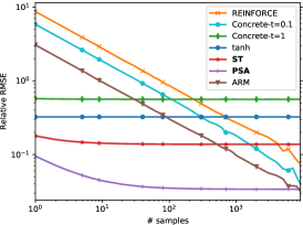
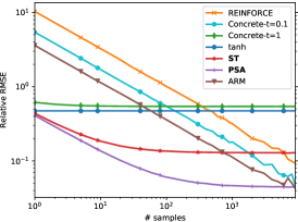
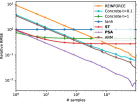
Figure 2: Root mean squared error of the gradient in layers 1 to 3 relative to the true gradient length after epoch 1 of training with reinforce. Layer 1 parameters correspond to $\theta^{1}$ in (1) – weights and biases defining preactivations of layer $1$ Bernoulli states. Unbiased estimators always improve with more samples. Biased estimators only improve up to a point. However, biased methods may be more accurate when using fewer samples and the discrepancy significantly increases with layer depth.

After 1 epoch	After 100 epochs	After 2000 epochs

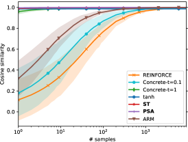
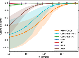
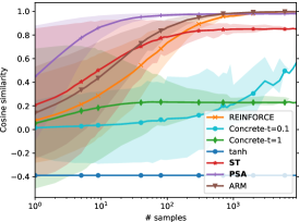
Figure 3: Cosine similarity of the estimated gradient to the true gradient in layer 1 at different points during training. The lines show the mean of the cosine similarity of the $N$-sample estimator. The shaded areas shows the interval containing 70% of the trials, illustrating the scatter of values that can be obtained in a random trial. It is seen that for some estimators there are good chances of failing to produce a positive cosine, i.e. a valid descent direction.

	No Augmentation	Affine Augmentation	Flip & Crop Augmentation
Training Loss
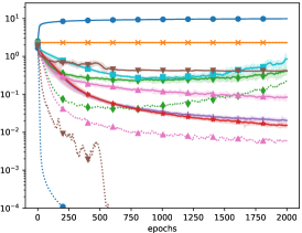
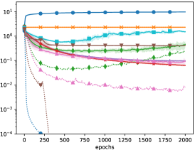
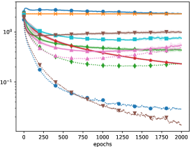
Validation Accuracy, %

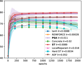
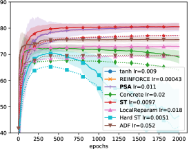
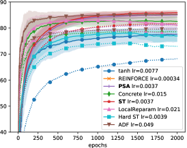
reinforce	Unbiased estimator [34].
Tanh	Replace $\operatorname{sign}(a-Z)$ by $E_{Z}[\operatorname{sign}(a-Z)]=\tanh(a/2)$.
Concrete-$t$	Concrete Relaxation [16] with the relaxation parameter $t$.
HardST	STE with the gradient of clamped identity, $\max(\min(a,1),-1)$.
ADF	Assumed density filtering, e.g., [27], the equivalent of PBNet method in [22] for real weights.
LocalReparam	Approximating pre-activations with normal distribution and sampling them.

Figure 4: Learning comparison on CIFAR-10. Solid loss curves measure the SBN expected loss. Doted loss curves indicate the relaxed objectives used by respective methods (where applicable). Solid accuracy curves are using 10-sample expected predictive probabilities of SBN and dotted curves only 1-sample predictive probabilities. All curves are smoothed over iterations and shaded areas denote $3{\times}$std w.r.t. smoothing. The automatically found learning rates are displayed in the legend.

Gradient Estimation Accuracy

To evaluate the accuracy of gradient estimators, we implemented the exact method, feasible for small models. We use the simple problem instance shown in Fig. B.1(a) with 2 classes and 100 training points per class in 2D and a classification network with 5-5-5 Bernoulli units. To study the bias-variance tradeoff we vary the number of samples used for an estimate and measure the Mean Squared Error (MSE). For unbiased estimators using $N$ samples leads to a straightforward variance reduction by $1/N$, visible in the log-log plot in Fig. 2 as straight lines. To investigate how the gradient quality changes with the layer depth we measure Root MSE in each of the 3 layers separately. It is seen in Fig. 2 that the proposed psa method has a bias, which is the asymptotic value of RMSE when increasing the number of samples. However, its RMSE accuracy with 1 sample is indeed not worse than that of the advanced unbiased arm method with $10^{3}$ samples. We should note that in more deterministic points, where the network converges to during the training, the conditions for approximation hold less well and the bias of psa may become more significant while unbiased methods become more accurate (but the gradient signal diminishes). Fig. 2 also confirms experimentally that psa is always more accurate than ST and has no bias in the last hidden layer, as expected. Additional experiments studying the dependence of accuracy on network width, depth and comparison with more unbiased baselines are given in Appendix C (Figs. C.5, C.6 and C.3). Both psa and ST methods are found to be in advantage when increasing depth and width.

The cosine similarity metric measured in Fig. 3 is more directly relevant for optimization. If it is close to one, we have an accurate gradient direction estimate. If it is positive, we still have a descent direction. Negative cosine similarity will seriously harm the optimization. For this evaluation we take the model parameters at epochs 1, 100 and 2000 of a reference training and measure the cosine similarity of gradients in layer 1. We see that methods with high bias may systematically fail to produce a descent direction while methods with high variance may produce wrong directions too often. Both effects can slow down the optimization or steer it wrongly.

The proposed psa method achieves the best accuracy in the practically important low-sample regime. The ST method is often found inferior and we know why: the extra linearization does not hold well when there are only few units in each layer. We expect it to be more accurate in larger models.

Deep Learning

To test the proposed methods in a realistic learning setting we use CIFAR-10 dataset and network with 8 convolutional and 1 fully connected layers (Appendix C). The first and foremost purpose of the experiment is to assess how the methods can optimize the training loss. We thus avoid using batch normalization, max-pooling and huge fully connected layers. When comparing to a number of existing techniques, we find it infeasible to optimize all hyper-parameters such as learning rate, schedule, momentum etc. per method by cross-validation. However, compared methods significantly differ in variance and may require significantly different parameters. We opt to use SGD with momentum with a constant learning rate found by an automated search per method (Appendix C). While this may be suboptimal, it nevertheless allows to compare the behavior of algorithms and analyze the failure cases. We further rely on SGD to average out noisy gradients with a suitable learning rate and therefore use 1-sample gradient estimates. To modulate the problem difficulty, we evaluate 3 data augmentation scenarios: no augmentation, affine augmentation, Flip&Crop augmentation.

Fig. 4 and Fig. C.1 show the training performance of evaluated methods. Both psa and st achieve very similar and stable training performance. This verifies that the extra linearization in st has no negative impact on the approximation quality in large models. For methods Tanh, Concrete, ADF, LocalReparam we can measure their relaxed objectives, whose gradients are used for the training (e.g. the loss of a standard neural network with $\tanh$ activations for Tanh). The training loss plots reveal a significant gap between these relaxed objectives and the expected loss of the SBN. While the relaxed objectives are optimized with an excellent performance, the real objective stalls or starts growing. This agrees with our findings in Fig. 3 that biased methods may fail to provide descent directions. HardST method, seemingly similar to our ST, performs rather poorly. Despite its learning rate is smaller than that of ST, it diverges in the first two augmentation cases, presumably due to wrongly estimated gradient directions. As we know from preceding work, good results with these existing methods are possible, in particular we also see that ADF with Flip&Crop augmentation achieves very good validation accuracy despite poor losses. We argue that in methods where bias may become high there is no sufficient control of what the optimization is doing and one needs to balance with empirical guessing. Finally, the reinforce method requires a very small learning rate in order not to diverge and the learning rate is indeed so small that we do not see the progress. We investigate if further by attempting input-dependent baselines in Section C.3. While it can optimize the objective in principle, the learning rate stays very small.

Please see further details on implementation and the training setup in Sections B.5 and C. The implementation is available at https://github.com/shekhovt/PSA-Neurips2020.

4 Conclusion

We proposed a new method for estimating gradients in SBNs, which combines an approximation by linearization and a variance reduction by summation along paths, both clearly interpretable. We experimentally verified that our psa method has a practical bias-variance tradeoff in the quality of the estimate, runs with a reasonable constant factor overhead, as compared to standard back propagation, and can improve the learning performance and stability. The st estimator obtained from psa gives the first theoretical justification of straight-through methods for deep models, opening the way for their more reliable and understandable use and improvements. Its main advantage is implementation simplicity. While the estimation accuracy may suffer in small models, we have observed that it performs on par with psa in learning large models, which is very encouraging. However, the influence of the systematic bias on the training is not fully clear to us, we hope to study it further in the future work.

Broader Impact

The work promotes stochastic binary networks and improves the understanding and efficiency of training methods. We therefore believe ethical concerns are not applicable. At the same time, developing more efficient training methods for binary networks, we believe may further increase the researchers and engineers interest in low-energy binary computations and aid progress in embedded applications such as speech recognition and vision. In the field of stochastic computing, which is rather detached at the moment, the stochasticity is treated as a source of errors and accumulators are used in every layer just to mimic smooth activation function [14, 15]. It appears to us that when stochastic binary computations are made useful instead, the related hardware designs can be made more efficient and stable w.r.t. to errors.

Path Sample-Analytic Gradient Estimators
for Stochastic Binary Networks (Appendix)

Appendix A Learning Formulations

Here we give a clarification on the learning formulation used in this work. During the training we consider the expected loss of a randomized predictor:

$$\mathbb{E}_{(x^{0},y)}\mathbb{E}_{Z}\big{[}F(\theta)\big{]}=-\mathbb{E}_{(x^{0},y)}{\color[rgb]{1,0,0}\mathbb{E}_{Z}}\big{[}\log p(y|X^{L};\theta)\big{]},$$ (15)

where $(x^{0},y)\sim\texttt{data}$. However at the test time we evaluate the expected predictor $\mathbb{E}_{Z}[p(y|X^{L};\theta)]$, considering $Z$ as latent variables, which can be interpreted as an ensemble of binary networks (see  Fig. B.1 c-f). The loss of this marginal predictor would be rather given by:

$$-\mathbb{E}_{(x^{0},y)}\big{[}\log{\color[rgb]{1,0,0}\mathbb{E}_{Z}}\big{[}p(y|X^{L};\theta)\big{]}\big{]}.$$ (16)

This setup is similar to dropout [28] with latent multiplicative Bernoulli noises. The expected loss (15) upper bounds the marginal loss (16) (by Jensen’s inequality), so that minimizing it also minimizes (16). However, unlike with dropout, the following observation holds for SBN models.

Proposition A.1.

In the family of models (1) with free scale and bias in all coordinates of $a^{k}$ there is always an effectively deterministic model (with no injected noises) that achieves the same or better expected loss (15).

This means that the model will tend to be deterministic and fit the classification boundary but not the data ambiguity (see Fig. B.1 b,c). Being aware of this, we note that it is nevertheless a common way to train classification models (e.g., dropout). Furthermore, the upper bound may be tightened by considering a multi-sample bound [30, 23] or variational bounds (applied for shallow models in [35, 9]). These extensions are left for future work as they require the ability to estimate gradients of the expected loss (15) in the first place. We can nevertheless see from the example in Fig. B.1 that the SBN family can be expressive when trained appropriately.

Appendix B Proofs

This section contains proofs, technical details and extended discussion that did not fit in the main paper.

B.1 Training with Expected Loss tends to Deterministic Models

See A.1 Raiko et al. [23] give a related theorem, but do not show the preferred deterministic strategy to be realizable in the model family.

Proof.

Let $\theta$ be parameters of the model optimizing (15). Let then $z^{*}$ be a maximizer of $\mathbb{E}_{(x^{0},y^{*})\sim\text{data}}\Big{[}f(x^{L}(z),y;\theta)\Big{]}$. Consider the case of a linear layer $a(x)=W^{T}x+b$ with the output $\operatorname{sgn}(W^{T}x+b-Z)$. Chose as new parameters $W^{\prime}=sW$, $b^{\prime}=s(b-z^{*})$ for $s\rightarrow\infty$. Since $Z$ has a finite variance, this ensures that $\operatorname{sgn}(W^{\prime T}X+b^{\prime}-Z)=\operatorname{sgn}(W^{T}X+b-z^{*}-Z/s)\rightarrow\operatorname{sgn}(W^{T}X+b-z^{*})$. The network with new weights is deterministic as it efficiently scales all noises to zero and it achieves same or better expected loss. The same argument applies whenever $a$ has a free scale and bias degrees of freedom. ∎

(a)

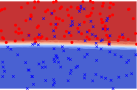
(b)

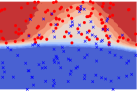
(c)

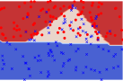
(d)

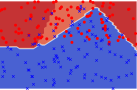
(e)

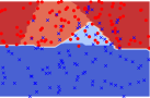
(f)

Figure B.1: Example problem to classify points in 2D with overlapping distributions. (a) Data points. (b) Classification model trained with the expected loss (15): the optimal solution tends to deterministic prediction. (c) Same model trained with a 10-sample bound [23], closer to the marginal likelihood (16). The model fits the uncertainty of the data. (d-f) Examples of the ensemble members obtained by fixing a particular realization of the noise variables $Z$ in all layer for the model in (c).

Let us remark that the conditions are not met in the following cases:

• The pre-activation does not have some degree of freedom, e.g., there is no bias term. This case is obvious.

• Pre-activations of different outputs do not have independent degrees of freedom per output. e.g., in a convolutional network we can suppress all the noises by scaling them down, however since the noises of all pre-activations are independent (not spatially identical), we cannot represent the bias from $z^{*}$ with the convolution bias which is spatially homogenous.

• The network uses parameter sharing in some other way, e.g., a Siamese network for matching.

These exceptions actually imply that training with expected loss a convolutional network in Section 3 tends to be deterministic but will not collapse to a fully deterministic state as it is suboptimal.

B.2 PSA Derivation and Properties

See 1

Proof.

Starting from LHS of (13) we take the sum in $x^{k}_{i}$ explicitly. The factors involving $x^{k}_{i}$ (after cancellation of the denominator with the respective term in $p(x)$) are

$$p(x^{k+1}|x^{k})J^{k}_{i}(x^{k}),$$ (17)

where we omit the dependance of $J^{k}_{i}$ on $x^{1\dots k-1}$, not relevant for the sum in $x^{k}_{i}$. Using the oddness of $J^{k}_{i}$, the sum of (17) in $x^{k}_{i}$ can be written as

$$\textstyle p(x^{k+1}|x^{k})J^{k}_{i}(x^{k})+p(x^{k+1}|x^{k}_{\downarrow i})J^{k}_{i}(x^{k}_{\downarrow i})=\big{(}p(x^{k+1}|x^{k})-p(x^{k+1}|x^{k}_{\downarrow i})\big{)}J^{k}_{i}(x^{k}).$$ (18)

Though this expression formally depends on $x^{k}_{i}$, it is by design invariant to $x^{k}_{i}$. Thus $x^{k}_{i}$ has been derandomized. We multiply (18) with $1=\sum_{x^{k}_{i}}p(x^{k}_{i}|x^{k-1})$ to obtain

$$\textstyle\sum_{x^{k}_{i}}p(x^{k}_{i}|x^{k-1})\big{(}p(x^{k+1}|x^{k})-p(x^{k+1}|x^{k}_{\downarrow i})\big{)}J^{k}_{i}(x^{k}),$$ (19)

which allows to put this expression back as a part of the joint sum in $x$ in (13). We thus obtain in (13):

$$\textstyle\sum_{i,x}p(x^{1\dots k})p(x^{k+2\dots L}|x^{k+1})\big{(}p(x^{k+1}|x^{k})-p(x^{k+1}|x^{k}_{\downarrow i})\big{)}J^{k}_{i}(x)f(x^{L}).$$ (20)

Recalling that $p(x^{k+1}|x^{k})=\prod_{j}p(x^{k+1}_{j}|x^{k})$, the product linearization (11) gives

$$\hskip-3.0pt\textstyle p(x^{k+1}|x^{k}){-}p(x^{k+1}|x^{k}_{\downarrow i})\approx\sum_{j}\frac{p(x^{k+1}|x^{k})}{p(x^{k+1}_{j}|x^{k})}\Delta^{k+1}_{i,j}(x),$$ (21)

where the division is used to represent the factor that needs to be excluded. Substituting this into (20) we get the resulting expression in (13). Finally, $\Delta^{k+1}_{i,j}(x)$ is odd in $x^{k+1}_{j}$ and $J^{k}(x)$ does not depend on $x^{k+1}_{j}$, and therefore $J^{k+1}_{j}$ is odd in $x^{k+1}_{j}$. ∎

Case $\bm{l{=}L}$

We now prove the expression (14) claimed as the derandomization result for the last layer when propagating $J^{L}$. Let us consider gradient in parameters of the last layer, $g^{L}$. In this case, the gradient expression (9) becomes

$$\textstyle\sum\limits_{x^{1\dots L-1}}p(x)\sum_{i}\sum\limits_{x^{L}}\frac{d^{L}_{i}(x)}{p(x^{L}|x^{L-1})}f(x^{L}).$$ (22)

Then derandomization over $x^{L}$ takes a particular simple form, which can be described by the following standalone lemma.

Lemma B.1.

Let $X_{i}$ be independent $\mathbb{B}$-valued Bernoulli with probability $p(x_{i};\theta)$ for $i=1\dots n$ and $f\colon\mathbb{B}^{n}\to\mathbb{R}$. Let $x$ be a joint sample and $x_{\downarrow i}$ denote the joint state with $x_{i}$ flipped. Then

$$\textstyle\sum_{i}\frac{\partial}{\partial\theta}p(x_{i};\theta)\big{(}f(x)-f(x_{\downarrow i})\big{)}$$ (23)

is an unbiased estimate of $\frac{\partial}{\partial\theta}\sum_{x}p(x;\theta)f(x)$.

Analogous results exist in the literature, e.g. [5] considers general discrete and continuous distributions.

Proof.

We differentiate the product of probabilities in the expectation:

$$\textstyle\frac{\partial}{\partial\theta}\sum\limits_{x}\prod\limits_{i}p(x_{i};\theta)f(x)=\sum\limits_{x}\sum\limits_{i}\frac{p(x)}{p(x_{i})}\frac{\partial}{\partial\theta}p(x_{i};\theta)f(x).$$ (24)

We then compute the sum over $x_{i}$ for each summand $i$ explicitly, obtaining

$$\textstyle\sum\limits_{i}\sum\limits_{x_{\lnot i}}p(x_{\lnot i})\frac{\partial}{\partial\theta}\Big{(}p(x_{i};\theta)f(x)+(1-p(x_{i};\theta))f(x_{\downarrow i})\Big{)},$$

where $x_{\lnot i}$ denotes excluding the component $i$. Since the expression in the brackets is invariant of $x_{i}$, we multiply by the factor $1=\sum_{x_{i}}p(x_{i})$ and get

$$\textstyle\sum_{x}p(x)\sum_{i}\big{(}f(x)-f(x_{\downarrow i})\big{)}\frac{\partial}{\partial\theta}p(x_{i}).$$ (25)

Thus (23) is a single sample unbiased estimate of (25). ∎

See 3

Proof.

The product linearization is not used anywhere in the method when we have a single binary unit in each hidden layer with $l<L$, nor it is used in the last layer. We therefore make no approximations and the 1-sample estimate is unbiased. ∎

B.3 Last Layer Enhancement

In Algorithm 1 Algorithm 1 we defined $E$ so that the gradient in $\theta^{L+1}$ is the common stochastic estimate $\frac{\partial f(x^{L};\theta^{L+1})}{\partial\theta^{L+1}}$. We now propose an improvement to this estimate. Intuitively, we want to utilize the values $f(x^{L}_{\downarrow i};\theta^{L+1})$ for all $i$ that we compute anyway.

Estimating $\sum_{x}p(x)\frac{\partial}{\partial\theta}f(x^{L};\theta)$ means to estimate the expected value of the function $g(x^{L})=\frac{\partial}{\partial\theta}f(x^{L};\theta)$, without further derivatives involved. We have the following lemma that applies derandomization over units in the last layer.

Lemma B.2.

Let $X_{i}$ be independent $\mathbb{B}$-valued Bernoulli with probability $p(x_{i})$ for $i=1\dots n$ and $g\colon\mathbb{B}^{n}\to\mathbb{R}$. Let $x$ be a joint sample. Then

$$\textstyle g(x)+\gamma\sum_{i}\big{(}g(x_{\downarrow i})-g(x)\big{)}(1-p(x_{i}))$$ (26)

is an unbiased estimate of $\mathbb{E}_{X}[g(X)]$.

Proof.

We expand for some fixed $i$:

$$\textstyle\mathbb{E}_{X}[g]=\sum_{x}p(x)g(x) \textstyle=\sum_{x_{\lnot i}}p(x_{\lnot i})\sum_{x_{i}}p(x_{i})g(x)$$ (27)

$$\textstyle=\sum_{x_{\lnot i}}p(x_{\lnot i})\Big{(}p(x_{i})g(x)+p(-x_{i})g(x_{\downarrow i})\Big{)}.$$ (28)

Observe that the bracket does not depend on $x_{i}$. We can therefore rewrite the expression as

$$\textstyle\sum_{x}p(x)\Big{(}p(x_{i})g(x)+p(-x_{i})g(x_{\downarrow i})\Big{)}$$ (29)

$$\textstyle= \textstyle\sum_{x}p(x)\Big{(}(1-p(-x_{i}))g(x)+p(-x_{i})g(x_{\downarrow i})\Big{)}$$ (30)

$$\textstyle= \textstyle\sum_{x}p(x)\Big{[}g(x)+\big{(}g(x_{\downarrow i})-g(x))p(-x_{i})\Big{]}.$$ (31)

This shows that

$$\sum_{x}p(x)\big{(}g(x_{\downarrow i})-g(x))p(-x_{i})=0.$$ (32)

So it serves as a variance reduction baseline. Moreover, if we have access to the two values $g(x_{\downarrow i})$ and $g(x)$, it is the perfect baseline, as adding it results in the complete sum in $x_{i}$. Taking the average over $i$, i.e. choosing $\gamma=\frac{1}{n}$ gives an estimate with a decreased variance, however it is not straightforward which value of $\gamma$ gives the best variance reduction as estimates (32) for all $i$ are not independent. ∎

Setting $\gamma=\frac{1}{n}$ is a natural choice that guarantees a reduction in variance. This improvement can be implemented as a simple replacement of the last line of the algorithm to:

$$\textstyle\pi^{L}_{i}=1-\operatorname{detach}((x^{L}_{i}+1)/2+x^{L}_{i}F_{Z}(a^{L}_{i}))$$ (33a)

$$\textstyle E=f(x^{L};\theta)+\sum\limits_{i}(f(x^{L};\theta){-}f(x^{L}_{\downarrow i};\theta))(q^{L}_{i}{-}\frac{\pi^{L}_{i}}{n}).$$ (33b)

B.4 Straight-Through

See 4

Proof.

Consider the last layer. The linear approximation to $f$ at $x^{L}$ allows to express

$$\textstyle f(x^{L}_{\downarrow i})\approx f(x^{L})+\frac{\partial f(x^{L})}{\partial x^{L}_{i}}(-2x^{L}_{i});$$ (34)

$$\textstyle df_{i}=f(x^{L})-f(x^{L}_{\downarrow i})\approx 2x^{L}_{i}\frac{\partial f(x^{L})}{\partial x^{L}_{i}}.$$ (35)

We use the expression for the derivative of layer probabilities in parameters (9)

$$D^{l}_{i}(x) \textstyle=p_{Z}(a^{l}_{i})x^{l}_{i}\frac{\partial}{\partial\theta^{l}}a^{l}_{i}(x^{l-1};\theta^{l})$$ (36)

and its oddness in $x^{l}_{i}$. The gradient in parameters of the last layer becomes

$$\textstyle\sum_{i}D^{L}_{i}df_{i}=\sum_{j}p_{Z}(a^{L}_{i})\frac{\partial}{\partial\theta^{L}}a^{L}_{i}(x^{L-1};\theta^{L})2\frac{\partial f(x^{L})}{\partial x^{L}_{i}},$$ (37)

where we have canceled $x^{L}_{i}x^{L}_{i}=1$.

With the linearization of $F_{Z}$ at $a^{k}$, the Jacobians $\Delta$ express linearly as follows:

$$\textstyle\Delta^{k}_{i,j}=x^{k}_{j}(F_{Z}(a^{k}_{j}){-}F_{Z}(a^{k}_{j\downarrow i}))\textstyle\approx x^{k}_{j}p_{Z}(a^{k}_{j})\big{(}a^{k}_{j}-a^{k}_{j\downarrow i}\big{)},$$ (38)

where $p_{Z}$ is the noise density, i.e. derivative of $F_{Z}$, and we have denoted $a^{k}_{j\downarrow i}=a^{k}_{j}(x^{k-1}_{\downarrow i};\theta^{k})$. Because $a^{k}$ is linear in $x^{k-1}_{i}$, we have similarly to (34) that

$$\textstyle a^{k}_{j}-a^{k}_{j\downarrow i}=2x^{k-1}_{i}\frac{\partial}{\partial x^{k-1}_{i}}a^{k}_{j}(x^{k-1}).$$ (39)

This allows to express

$$\textstyle\Delta^{k}_{i,j}=2x^{k}_{j}x^{k-1}_{i}p_{Z}(a^{k}_{j})\frac{\partial}{\partial x^{k-1}_{i}}a^{k}_{j}(x^{k-1})=2x^{k}_{j}x^{k-1}_{i}\frac{\partial}{\partial x^{k-1}_{i}}F_{Z}(a^{k}(x^{k-1})).$$ (40)

Note the occurrence of the formal derivative of $F_{Z}(a^{k}(x^{k-1}))$ in $x^{k-1}_{i}$, that will be the only derivative that is used in the ST algorithm.

Finally observe that for the derivative in parameters of layer $l$, estimated with the product $D^{l}\Delta^{l+1}\cdot\dots\cdot\Delta^{L}df$ in PSA, for each $k\geq l$ the factors $x^{k}_{i_{k}}$ appear exactly twice and thus cancel. We recover the product of Jacobians without extra multipliers by $x^{k}_{i_{k}}$, which can be implemented with automatic differentiation as proposed in Algorithm 2. ∎

The connection to STE pointed out by [32] can be seen as a special case of our construction for a single hidden layer, where local expectation gradients [31] apply and it suffices to linearize $f$.

B.5 Complexity and Efficient Implementation of PSA

We have made the following complexity claim. See 2 For fully connected networks this complexity is indeed linear in the total number of inputs and weights. For convolutional networks it is a bit more tricky because convolutions can generate big output tensors. In this case the complexity can be stated as linear in the total number of inputs, weights and hidden units.

We prove the claim by giving the algorithms how to implement all necessary computations with the same complexity as standard back-propagation.

First, we observe that the numbers $q$ in Algorithm 1 are only used to determine the derivative and set to zero value by line (1). The pre-activations $a$ in Algorithm 1 are of the same form as in the standard network, evaluating $F_{Z}$ component-wise does not increase complexity. Therefore backpropagation for these parts takes the same time. We only need to additionally compute the matrices $\Delta$ on the backward pass and explicitly implement the transposed multiplication (resp. transposed convolution) with them to define a custom backprop operation for the update (1).

Fully Connected Layers

Consider the case of a fully connected layer with pre-activation $a(x)=Wx+b$. Then $\Delta_{ij}$ has the same size as the matrix $W$. Recall it expresses as

$$\textstyle\Delta_{i,j}=x^{k}_{j}\Big{(}F_{Z}(a_{j})-F_{Z}(a_{j}(x^{k-1}_{\downarrow i}))\Big{)}.$$ (41)

The first summand can be computed in linear time once $x^{k}$ and $a$ are known. The second summand is slightly more complex as it involves pre-activations for inputs with a flipped component $i$. For linear layers we have:

$$a_{j}(x^{k-1}_{\downarrow i})=Wx^{k-1}_{\downarrow i}+b=a_{j}-2W_{j,i}x_{i},$$ (42)

i.e. all the numbers $a_{j}(x^{k-1}_{\downarrow i})$ can be computed in time $O(n_{k}n_{k-1})$ for a matrix $W\in\mathbb{R}^{n_{k}\times n_{k-1}}$. It follows that computing matrix $\Delta$ takes $O(n_{k}n_{k-1})$ time, the same as the matrix-vector multiplication $Wx^{k-1}$ for forward pass or the transposed multiplication for the backward pass.

Convolutional Layer

With a convolutional layer, the implementation is more tricky, because computing $\Delta$ in a matrix form is no longer efficient. Consider the convolution pre-activation

$$a_{o,j}=\sum_{c,@i}w_{o,c,i-j}x_{c,i},$$ (43)

where $c$ and $o$ are input and output channels, $i$ and $j$ are 2d indices of spatial locations and $@i$ denotes that the range of $i$ is given by the output location $j$ and the weight kernel size: $j-h/2\leq i\leq j+h/2$. This notation makes it more easier to match with the equations in the matrix form.

For the gradient in the standard network, a transposed convolution occurs:

$$\frac{\partial}{\partial x^{k-1}_{c,i}}=\sum_{o,@j}w_{o,c,j-i}\frac{\partial}{\partial x^{k}_{o,j}}.$$ (44)

For the gradient in PSA, we need to implement the following sum with $\Delta$:

$$\frac{\partial}{\partial q^{k-1}_{c,i}}=\sum_{o,j}\Delta_{o,c,j,i}\frac{\partial}{\partial q^{k}_{o,j}},$$ (45)

where in the case of convolution and symmetric noise, $\Delta$ is given by

$$\Delta_{o,c,j,i}=x^{k}_{o,j}\Big{(}F_{Z}(a_{o,j})-F_{Z}(a_{o,j}(x^{k-1}_{c,\downarrow i}))\Big{)}.$$ (46)

Using that $a_{o,j}(x^{k-1}_{c,\downarrow i})$ itself is given by the convolution, we have

$$a_{o,j}(x^{k-1}_{c,\downarrow i})=\begin{cases}a_{o,j}-2w_{o,c,i-j}x^{k-1}_{c,i},&\mbox{ \rm if }-h/2\leq i\leq h/2;\\ a_{o,j},&\mbox{ \rm otherwise}.\end{cases}$$ (47)

Therefore $\Delta_{o,c,j,i}$ has the same support in indices $i,j$ as the convolution, but it is different in that it cannot be represented as just a function of $i-j$. It can be interpreted as a convolution with a kernel, which is spatially varied, i.e. at all locations a different kernel is applied.

Due to the structure of $\Delta$, the sum (45) takes the same range of indices as the convolution, we may write:

$$\frac{\partial}{\partial q^{k-1}_{c,i}}=\sum_{o,@j}\Delta_{o,c,j,i}\frac{\partial}{\partial q^{k}_{o,j}}.$$ (48)

The elements of the kernel $\Delta_{o,c,j,i}$ are computed in $O(1)$ time, therefore the full backprop operation (45) has the same complexity as backprop with standard network (assuming small kernel size, where convolution uses straightforward implementation and not FFT).

We take one step further, to show that convolution with $\Delta$ for logistic noise needs literally the same amount of operations. Computing the convolution (45) with the first summand of $\Delta$ is easy. As it does not involve the index $i$, it reduces to multiplication in the output space (indices $o,j$), summation over $o$ and a convolution with just the support indicator in $j$.

It remains to compute the convolution (50) with the second summand of $\Delta$, i.e.:

$$\sum_{o,@j}x^{k}_{o,j}F_{Z}(a_{o,j}-2w_{o,c,i-j}x^{k-1}_{c,i})g_{o,j},$$ (49)

where we denoted the gradient w.r.t. the output as $g$. The factor $x^{k}_{o,j}$ is easily accounted for, by introducing $\tilde{g}_{o,j}=g_{o,j}x^{k}_{o,j}$. We can further expand for logistic noise:

$$\sum_{o,@j}\frac{1}{1+e^{a_{o,j}}e^{-2w_{o,c,i-j}x^{k-1}_{c,i}}}\tilde{g}_{o,j}.$$ (50)

Since $x^{k-1}_{c,i}$ takes only two possible values, for each input gradient coordinate $c,i$ we need the convolution with $e^{\pm 2w_{o,c,i-j}}$. We can precompute $A_{o,j}=\exp(a_{o,j})$, $W^{\pm}_{o,c,l}=\exp(\pm 2w_{o,c,i-j})$, i.e. the expensive $\exp$ operations need to be performed only for the output and the kernel alone, and not inside the convolution. For the dominant complexity part involving $c,o,i,@j$ indices, we only need to compute and aggregate

$$\sum_{o,@j}\frac{\tilde{g}_{o,j}}{1+A_{o,j}W^{\pm}_{o,c,i-j}}.$$ (51)

Compared to standard convolution, this costs only one extra addition and division operation. We call the operation (51) a ratio convolution and implemented it in CUDA. Since our implementation is not fully optimized and we need to load twice as much data ($g$ and $A$) for the input and $W^{\pm}$ for the “kernel”, the actual run-time is 3-4 times slower than that of cuDNN standard convolution.

Head Function

For the head function $f(x^{L})$ that is a composition of a linear layer $Wx^{L}+b$ and some fixed function $h$, in order to compute $f(x^{L})-f(x^{L}_{\downarrow i})$ we need again to form all pre-activations $a_{j}(x^{L}_{\downarrow i})$ that takes $O(n_{L}K)$ time, where $K$ is the number of classes (more generally, the dimensionality of the network output). This is of the same size as the matrix $W$. Assuming that the final loss function $h\colon\mathbb{R}^{K}\to\mathbb{R}$ (e.g., cross-entropy) takes time $O(K)$, the computation in the last layer has complexity $O(n_{L}K)$ as we need to call this function for all input flips. This is however still of the same complexity as size of the matrix $W$.

Appendix C Details of Experiments and Additional Comparisons

In this section we describe details of the experimental setup and measuring techniques and offer some auxiliary experiments.

C.1 Gradient Estimation Accuracy

We use the simple problem instance shown in Fig. B.1(a) with 2 classes and 100 training points per class in 2D and a classification network with 5-5-5 Bernoulli units. The data was generated as follows. Points of class 1 (resp. 2) are uniformly distributed above $y=0$ (resp. below $y=\cos(x)$) for $x\in[-\pi/2,\pi/2]$. The implementation is available in gradeval/expclass.py. We have experimented with several configurations varying the number of units and layers. Generally, with a smaller number of units arm gets more accurate and st gets less accurate, but the overall picture stays. We therefore demonstrate the comparison on the 5-5-5 configuration.

The training progress is shown in Fig. C.2. In this problem unbiased estimators perform well and an extra variance reduction of PSA is not essential. To measure RMSE and cosine similarity errors in Fig. 2, we collect $T=10^{4}$ total samples for each estimator. For each value of the number of samples $M$ shown on the x-axis, we calculate the mean and variance of an $M$-sample estimator by using the $T/M$ sample groups to estimate these statistics. The same $T$ samples are used to estimate the values for varying $M$. Towards $M\rightarrow T$ the estimates become more noisy, so the rightmost parts of the plots shouldn’t be considered reliable.

Comparisons with additional unbiased methods is proposed in Fig. C.3 and Fig. C.4. We compare to the following techniques: 1. reinforce with the constant input-dependent baseline set to the true expected function value of the loss objective per data sample. This choice represents the best of what one can expect to get with input-dependent baselines constant or trained with a neural network as NVIL [18]. 2. MuProp [10], which uses a linear baseline around deterministically propagated points. The constant part of the baseline may also optionally set to the input-dependent true value. It is seen from the results that the linear baseline of MuProp does not improve accuracy in deep layers, possibly connected to the fact that the loss depends only on the state of the last layer and thus its linear approximation using states of the first layers is not helpful. It is also seen in Fig. C.4 that the linear baseline of MuProp degrades at 2000 epochs. For this experiment we used only $T=2000$ samples.

C.2 Deep Learning

	No Augmentation	Affine Augmentation	Flip & Crop Augmentation
Validation Loss
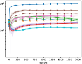
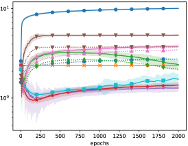
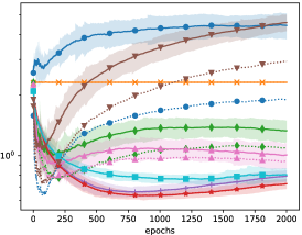
Training Accuracy

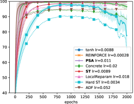
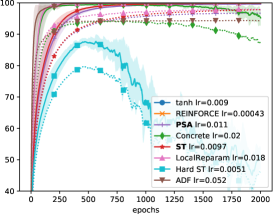
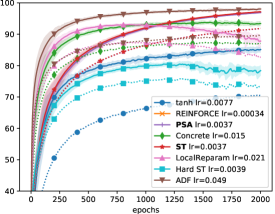
Figure C.1: Additional plots to Fig. 4: validation losses and training accuracies.

Dataset

The learning experiments are performed on CIFAR10 dataset. The dataset contains a training set and a test set. Following the common approach, we withhold 5000 samples (10 percent) of the training set as a validation set. Since we do not perform any hyper-parameter tuning or model selection based on the validation set, it provides an independent and unbiased estimates.

Augmentation

For Affine augmentation experiment we used random affine transforms that included shifts by $\pm 5\%$ and rotation by $\pm 10\deg$, linearly interpolated. Flip&Crop is the commonly applied augmentation for this dataset. It consists of random horizontal flips and random shifts with zero padding by $\pm 4$ pixels (transforms.RandomCrop(32, 4)). Fro the training plots and loss values achieved we can hypothesize that this augmentation is more "diverse" and harder to fit that the Affine augmentation above.

Network

For simplicity, we used a variant of All convolutional network (Springenberg et al. 2014), with strides instead of max pooling. The network structure is as follows:

⬇

ksize = [3, 3, 3, 3, 3, 3, 3, 1 ]

stride= [1, 1, 2, 1, 1, 2, 1, 1 ]

depth = [96, 96, 96, 192, 192, 192, 192, 192]

There is no padding and the output is a $192\times 2\times 2$ binary tensor, which is then flattened and passed to the head function consisting of an affine transform to the $10$-dimensional class logits. This network is smaller than VGG-type networks commonly used [12], however significantly smaller is size esp. considering the last fully connected layer. Our FC has size $768{\times}10$, the ones in [12] (there are three) are: $8192{\times}1024$, $1024{\times}1024$, $1024{\times}10$. No batch normalization is used for the purity of comparison experiments. If we were chasing the highest accuracy, we can confirm that BN improves the results.

Optimizer

For the optimization we used batch size 64 and SGD optimizer with Nesterov Momentum 0.9 (pytorch default) and a constant learning rate. Because different methods have different variance and biases, for a fair comparison we tried to find the optimal learning rate for each method individually. We selected the learning rate by a numerical optimization based on the performance of the model in 5 epochs as measured by the objective optimized by the method (i.e. the sample-based estimate of the expected loss or the approximated expected loss) on the training set. We used exponentially weighted average on the objective value to reduce its variance. We used

⬇

scipy.optimize.minimize_scalar(f, method=’bounded’, bounds=(-6, 0),maxiter=10)

for the numerical search of the optimal $\log$ of the learning rate. Arguably, this learning rate selection optimizing the short-horizon performance may be sub-optimal in a longer run, but is the first best approximation to deal with this issue.

Parameters of linear and convolutional layers were initialized as uniformly distributed. We then perform one iteration, computing mean and variance statistics over a batch and spatial dimensions and whitening pre-activations using these statistics, similar to batch normalization. This is performed only as a data-dependent initialization to make sure that activations are in a reasonable range on average and the gradients are initially non-vanishing.

Test Metrics

In our experiments all hyperparameters including the learning rates are tuned exclusively on the training set as detailed above. Hence the validation set provides an unbiased estimate of the test error and we report only it.

Methods

Here we specify additional details on the baseline methods used in the learning experiment. The ADF method, called AP2 in [26], propagates means and variances through the hidden layers fully analytically. This method is the equivalent of the PBNet method in [22] when the weights are deterministic. We only sample the states of the last binary layer are sampled, as a general solution suitable with different head functions. The ADF family of methods includes expectation propagation [17] designed for approximate variational inference in graphical models. It computes an approximation to summation (5) by fitting and propagating a fully factorized approximation to marginal distributions $p(x^{k}|x^{0})$ with forward KL divergence. The gradient of this approximation is then evaluated. The PSA method differs in that it approximates the gradient directly and does not make a strong factorization assumption. From the experiments we observe that ADF performs very well in the beginning, when all weights are initially random and then it over-fits to the relaxed objective.

In the LocalReparam method we sample pre-activations from their approximated Normal distribution and computed probabilities of the outputs analytically. This is related but different from the PBNet-S method [22], which samples activations from the concrete relaxation distribution and is not directly applicable to real-valued deterministic weights. The implementation of our methods and these baselines is available.

Infrastructure

The experiments were run on linux servers with NVIDIA GTX1080 cards and Tesla P100 cards.

Running Time

We measure running time for a single batch of size 64 and the running time for one epoch of training / validation. The training loop includes measuring statistics using 10 samples of the model per data point, which increases amount of forward computations performed. Please consider that these numbers are indicative only, as we did not optimize for performance beyond providing the CUDA kernel for psa. We also have lots of overhead from implementing padding and strides in pytorch, externally to the kernel. Times are given in seconds.

Method	Forward batch	Backward batch	Train Epoch with measurements	Val Epoch with measurements
PSA	0.013	0.056	105	14
Gumbel	0.009	0.012	77	13
Tanh	0.005	0.011	77	12.5
REINFORCE	0.014	0.009	77	14
ADF	0.012	0.031	91.5	14
LocalReparam	0.015	0.029	98	14
ST	0.009	0.011	77	13
HardST	0.009	0.011	77	13

C.3 MuProp and REINFORCE with Baselines

For fairness of comparison we have additionally tried to use reinforce with a centering variance reduction and MuProp. As a baselines for these methods we use the exponentially weighted average (EWA) of the loss function per data point with momentum=0.9. Since the learning rate needed for these methods is rather small, the EWA is close to the true expected loss value per data point. Since the EWA is kept per data point, this is an accurate input-dependent constant baseline. We made several learning trials with automatically selected learning rates (denoted with stars in Fig. C.7) as well as manually set learning rates. Since automatic learning rates appear to be too high as they lead do divergence, it only makes sense to decrease these learning rates. We tried setting the learning rates smaller. The results in Fig. C.7 show that with some careful choice of parameters, reinforce and MuProp can make progress. However, the learning rates required are 1-2 orders smaller than with biased methods, which leads to much slower performance. Indeed, comparing Fig. C.7 and Fig. 4 (note the scale difference of $y$-axis), we observe that variance-reduced reinforce and MuProp in 1000 epochs have barely made the progress of biased estimators in 10 epochs.

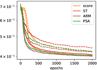
Figure C.2: Training losses when training a small network 5-5-5 on the data in Fig. B.1(a) with several methods. Here the dashed curves show the SBN objective, the expected loss of randomized predictor (15), which upper bounds the the loss of the ensemble (15) shown with solid curves. We see that reinforce (score) does not do very well in the beginning, but eventually gets into a mode that allows it to optimize the objective. The methods arm and psa perform similar and st is somewhat slower due to its bias for this small model.

Layer 1	Layer 2	Layer 3

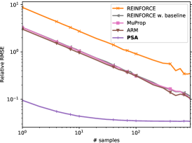
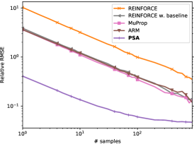
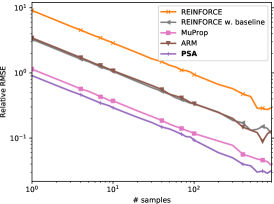
Figure C.3: Root mean squared error of the gradient in layers 1 to 3 relative to the true gradient length after epoch 1. Comparisons with more unbiased methods in the same setting as Fig. 2.

After 1 epoch	After 100 epochs	After 2000 epochs

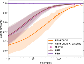
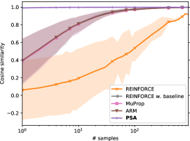
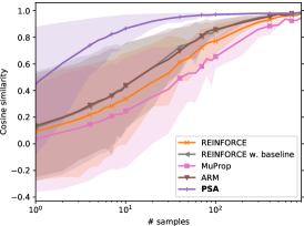
Figure C.4: Cosine similarity of the estimated gradient to the true gradient in layer 1 at different points during training. Comparisons with more unbiased methods in the same setting as Fig. 3.

3-3-3	5-5-5	10-10-10

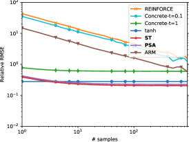
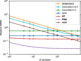
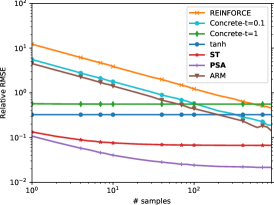
Figure C.5: Dependence on the network width. Shown gradient RMES in Layer 1 after epoch 1 (close to randomly initialized network). Bias of PSA and ST is more prominent in small models.

2 layers	5 layers	7 layers

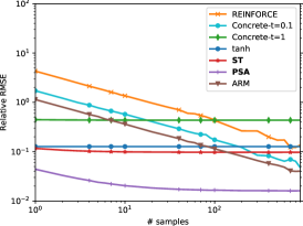
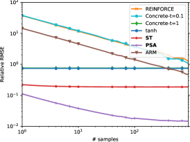
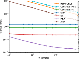
Figure C.6: Dependence on the network depth. Shown gradient RMES in Layer 1 after epoch 1 (close to randomly initialized network). The variance of unbiased estimators grows much faster when increasing the network depth. The network width is fixed to 5 units per layer.

	Flip & Crop Augmentation
Training Loss

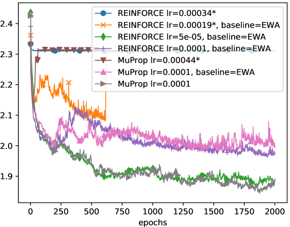
Figure C.7: Performance of reinforce and MuProp with different learning rates and input-dependnet constant baselines estimated using a running averages. No smoothing is applied across epochs in this plot. Note the limits of $y$-axis in comparison to Fig. 3.

References

- Bengio et al. [2013] Bengio, Y., Léonard, N., and Courville, A. Estimating or propagating gradients through stochastic neurons for conditional computation. arXiv preprint arXiv:1308.3432, 2013.
- Bethge et al. [2018] Bethge, J., Bornstein, M., Loy, A., Yang, H., and Meinel, C. Training competitive binary neural networks from scratch. CoRR, abs/1812.01965, 2018.
- Cassidy et al. [2016] Cassidy, A. S., Sawada, J., Merolla, P., Arthur, J. V., Alvarez-Icaza, R., Akopyan, F., Jackson, B. L., and Modha, D. S. Truenorth: A high-performance, low-power neurosynaptic processor for multi-sensory perception, action, and cognition. 2016.
- Cheng et al. [2019] Cheng, P., Liu, C., Li, C., Shen, D., Henao, R., and Carin, L. Straight-through estimator as projected wasserstein gradient flow. arXiv preprint arXiv:1910.02176, 2019.
- Cong et al. [2019] Cong, Y., Zhao, M., Bai, K., and Carin, L. GO gradient for expectation-based objectives. In International Conference on Learning Representations, 2019.
- Courbariaux et al. [2016] Courbariaux, M., Hubara, I., Soudry, D., El-Yaniv, R., and Bengio, Y. Binarized neural networks: Training deep neural networks with weights and activations constrained to+ 1 or-1. arXiv preprint arXiv:1602.02830, 2016.
- Davies et al. [2018] Davies, M., Srinivasa, N., Lin, T., Chinya, G., Cao, Y., Choday, S. H., Dimou, G., Joshi, P., Imam, N., Jain, S., Liao, Y., Lin, C., Lines, A., Liu, R., Mathaikutty, D., McCoy, S., Paul, A., Tse, J., Venkataramanan, G., Weng, Y., Wild, A., Yang, Y., and Wang, H. Loihi: A neuromorphic manycore processor with on-chip learning. IEEE Micro, 38(1):82–99, January 2018.
- Gast & Roth [2018] Gast, J. and Roth, S. Lightweight probabilistic deep networks. In CVPR, June 2018.
- Grathwohl et al. [2018] Grathwohl, W., Choi, D., Wu, Y., Roeder, G., and Duvenaud, D. Backpropagation through the void: Optimizing control variates for black-box gradient estimation. In ICLR, 2018.
- Gu et al. [2016] Gu, S., Levine, S., Sutskever, I., and Mnih, A. Muprop: Unbiased backpropagation for stochastic neural networks. In 4th International Conference on Learning Representations (ICLR), May 2016.
- Hinton [2012] Hinton, G. Lecture 15d - semantic hashing : 3:05 - 3:35, 2012. URL https://www.cs.toronto.edu/~hinton/coursera/lecture15/lec15d.mp4.
- Hubara et al. [2016] Hubara, I., Courbariaux, M., Soudry, D., El-Yaniv, R., and Bengio, Y. Binarized neural networks. In Lee, D. D., Sugiyama, M., Luxburg, U. V., Guyon, I., and Garnett, R. (eds.), Advances in Neural Information Processing Systems 29, pp. 4107–4115. 2016.
- Jang et al. [2016] Jang, E., Gu, S., and Poole, B. Categorical reparameterization with gumbel-softmax. arXiv preprint arXiv:1611.01144, 2016.
- Kim et al. [2016] Kim, K., Kim, J., Yu, J., Seo, J., Lee, J., and Choi, K. Dynamic energy-accuracy trade-off using stochastic computing in deep neural networks. In ACM/EDAC/IEEE Design Automation Conference (DAC), pp. 1–6, 2016.
- Lee et al. [2017] Lee, V. T., Alaghi, A., Hayes, J. P., Sathe, V., and Ceze, L. Energy-efficient hybrid stochastic-binary neural networks for near-sensor computing. In Proceedings of the Conference on Design, Automation & Test in Europe, DATE ’17, pp. 13–18, 3001 Leuven, Belgium, Belgium, 2017. European Design and Automation Association. URL http://dl.acm.org/citation.cfm?id=3130379.3130383.
- Maddison et al. [2016] Maddison, C. J., Mnih, A., and Teh, Y. W. The concrete distribution: A continuous relaxation of discrete random variables. 2016. arxiv:1611.00712.
- Minka [2001] Minka, T. P. Expectation propagation for approximate Bayesian inference. In Uncertainty in Artificial Intelligence, pp. 362–369, 2001.
- Mnih & Gregor [2014] Mnih, A. and Gregor, K. Neural variational inference and learning in belief networks. In Proceedings of the 31st International Conference on Machine Learning, volume 32, pp. 1791–1799, 22–24 Jun 2014.
- Neal [1992] Neal, R. M. Connectionist learning of belief networks. Artif. Intell., 56(1):71–113, July 1992.
- Owen [2013] Owen, A. B. Monte Carlo theory, methods and examples. 2013.
- Paszke et al. [2019] Paszke, A., Gross, S., Massa, F., Lerer, A., Bradbury, J., Chanan, G., Killeen, T., Lin, Z., Gimelshein, N., Antiga, L., Desmaison, A., Kopf, A., Yang, E., DeVito, Z., Raison, M., Tejani, A., Chilamkurthy, S., Steiner, B., Fang, L., Bai, J., and Chintala, S. Pytorch: An imperative style, high-performance deep learning library. In Advances in Neural Information Processing Systems 32, pp. 8024–8035. 2019.
- Peters et al. [2019] Peters, J. W., Genewein, T., and Welling, M. Probabilistic binary neural networks, 2019. URL https://openreview.net/forum?id=B1fysiAqK7.
- Raiko et al. [2015] Raiko, T., Berglund, M., Alain, G., and Dinh, L. Techniques for learning binary stochastic feedforward neural networks. In ICLR, 2015. URL http://arxiv.org/abs/1406.2989.
- Rastegari et al. [2016] Rastegari, M., Ordonez, V., Redmon, J., and Farhadi, A. XNOR-Net: Imagenet classification using binary convolutional neural networks. In ECCV, volume 9908, pp. 525–542. Springer, 2016.
- Roth et al. [2019] Roth, W., Schindler, G., Fröning, H., and Pernkopf, F. Training discrete-valued neural networks with sign activations using weight distributions. In European Conference on Machine Learning (ECML), 2019.
- Shekhovtsov & Flach [2018] Shekhovtsov, A. and Flach, B. Normalization of neural networks using analytic variance propagation. In Computer Vision Winter Workshop, pp. 45–53, 2018.
- Shekhovtsov & Flach [2019] Shekhovtsov, A. and Flach, B. Feed-forward propagation in probabilistic neural networks with categorical and max layers. In International Conference on Learning Representations, 2019. URL https://openreview.net/forum?id=SkMuPjRcKQ.
- Srivastava et al. [2014] Srivastava, N., Hinton, G., Krizhevsky, A., Sutskever, I., and Salakhutdinov, R. Dropout: A simple way to prevent neural networks from overfitting. JMLR, 15:1929–1958, 2014.
- Tang et al. [2017] Tang, W., Hua, G., and Wang, L. How to train a compact binary neural network with high accuracy? In AAAI, 2017.
- Tang & Salakhutdinov [2013] Tang, Y. and Salakhutdinov, R. R. Learning stochastic feedforward neural networks. In Burges, C. J. C., Bottou, L., Welling, M., Ghahramani, Z., and Weinberger, K. Q. (eds.), NeurIPS, pp. 530–538. 2013.
- Titsias & Lázaro-Gredilla [2015] Titsias, M. K. and Lázaro-Gredilla, M. Local expectation gradients for black box variational inference. In NeurIPS, pp. 2638–2646, 2015.
- Tokui & Sato [2017] Tokui, S. and Sato, I. Evaluating the variance of likelihood-ratio gradient estimators. In Proceedings of the 34th International Conference on Machine Learning - Volume 70, pp. 3414–3423, 2017.
- Tucker et al. [2017] Tucker, G., Mnih, A., Maddison, C. J., Lawson, J., and Sohl-Dickstein, J. Rebar: Low-variance, unbiased gradient estimates for discrete latent variable models. In Guyon, I., Luxburg, U. V., Bengio, S., Wallach, H., Fergus, R., Vishwanathan, S., and Garnett, R. (eds.), NeurIPS, pp. 2627–2636. 2017.
- Williams [1992] Williams, R. J. Simple statistical gradient-following algorithms for connectionist reinforcement learning. Machine Learning, 8(3):229–256, May 1992.
- Yin & Zhou [2019] Yin, M. and Zhou, M. ARM: Augment-REINFORCE-merge gradient for stochastic binary networks. In ICLR, 2019.
- Yin et al. [2019] Yin, P., Lyu, J., Zhang, S., Osher, S., Qi, Y., and Xin, J. Understanding straight-through estimator in training activation quantized neural nets. arXiv preprint arXiv:1903.05662, 2019.
- Zhou et al. [2016] Zhou, S., Wu, Y., Ni, Z., Zhou, X., Wen, H., and Zou, Y. Dorefa-net: Training low bitwidth convolutional neural networks with low bitwidth gradients. arXiv preprint arXiv:1606.06160, 2016.