$N$-jettiness beam functions at N³LO

Abstract

We present the first complete calculation for the quark and gluon $N$-jettiness ($\mathcal{T}_{N}$) beam functions at next-to-next-to-next-to-leading order (N³LO) in perturbative QCD. Our calculation is based on an expansion of the differential Higgs boson and Drell-Yan production cross sections about their collinear limit. This method allows us to employ cutting edge techniques for the computation of cross sections to extract the universal building blocks in question. The class of functions appearing in the matching coefficents for all channels includes iterated integrals with non-rational kernels, thus going beyond the one of harmonic polylogarithms. Our results are a key step in extending the $\mathcal{T}_{N}$ subtraction methods to N³LO, and to resum $\mathcal{T}_{N}$ distributions at N³LL^′ accuracy both for quark as well as for gluon initiated processes.

1 Introduction

Experimental measurements at the LHC have provided remarkably precise measurements for a multitude of observables, most notably weak gauge boson production, an important benchmark for the Standard Model which has been measured at percent level accuracy Aaboud:2017svj ; Aaboud:2017ffb ; Khachatryan:2016nbe ; Sirunyan:2019bzr . Strong constraints on physics beyond the Standard Model are also provided by precision measurements of Higgs boson production and diboson processes Sirunyan:2018koj ; Aad:2020mkp ; Aaboud:2019nkz ; Aaboud:2019lgy ; Sirunyan:2019gkh . To make full use of these results, it is crucial to confront them with equally-precise theory predictions, which in particular requires to include higher-order corrections in QCD.

So far, only inclusive Drell-Yan and Higgs production have been calculated at next-to-next-to-next-to-leading order (N³LO) in QCD Anastasiou:2014vaa ; Anastasiou:2015ema ; Dreyer:2016oyx ; Dreyer:2018qbw ; Mistlberger:2018etf ; Duhr:2019kwi ; Duhr:2020kzd ; Duhr:2020seh , while significant progress is being made to reach the same precision for differential distributions Cieri:2018oms ; Dulat:2018bfe . A key challenge for such calculations is the cancellation of infrared divergences between real and virtual corrections, and hence a necessary prerequisite is a profound understanding of the infrared singular structure at three loops.

$N$-jettiness ($\mathcal{T}_{N}$) is an infrared-sensitive $N$-jet resolution observable and thus provides a way to study the singular structure of QCD Stewart:2009yx ; Stewart:2010tn . Its simplest manifestation $\mathcal{T}_{0}$, also referred to as beam thrust, is defined as

$$\mathcal{T}_{0}=\sum_{i}\min\biggl{\{}\frac{2q_{a}\cdot k_{i}}{Q_{a}}\,,\frac{2q_{b}\cdot k_{i}}{Q_{b}}\biggr{\}}\,,$$ (1)

where the sum rums over all momenta $k_{i}$ in the hadronic final state, $q_{a,b}$ are the momenta of the incoming partons projected onto the Born kinematics, and the measures $Q_{a,b}$ distinguish different definitions of $\mathcal{T}_{0}$ Stewart:2010pd ; Jouttenus:2011wh . A key feature of $\mathcal{T}_{N}$ is that its singular structure as $\mathcal{T}_{N}\to 0$ is fully captured by a factorization theorem, as shown in refs. Stewart:2009yx ; Stewart:2010tn using soft-collinear effective theory (SCET) Bauer:2000ew ; Bauer:2000yr ; Bauer:2001ct ; Bauer:2001yt ; Bauer:2002nz . In the simplest case, namely the production of a color-singlet final state $h$, the appropriate factorization theorem reads

$$\frac{\mathrm{d}\sigma}{\mathrm{d}Q^{2}\mathrm{d}Y\mathrm{d}\mathcal{T}_{0}} =\sigma_{0}\sum_{a,b}H_{ab}(Q^{2},\mu)\int\!\mathrm{d}t_{a}\,\mathrm{d}t_{b}\,B_{a}(t_{a},x_{a},\mu)\,B_{b}(t_{b},x_{b},\mu)\,S_{c}\Bigl{(}\mathcal{T}_{0}-\frac{t_{a}}{Q_{a}}-\frac{t_{b}}{Q_{b}},\mu\Bigr{)}$$

$$\quad\times\Bigl{[}1+\mathcal{O}\Bigl{(}\frac{\mathcal{T}_{0}}{Q}\Bigr{)}\Bigr{]}\,.$$ (2)

Here, $Q^{2}$ and $Y$ are the invariant mass and rapidity of $h$, respectively, and we normalize by the Born partonic cross section $\sigma_{0}$. In eq. (1), the full process dependence is given in terms of the hard function $H_{ab}$, which encodes virtual corrections to the underlying hard process $ab\to h$. The beam functions $B_{a,b}$ encode radiation collinear to the incoming partons. The soft function $S_{c}$ encodes soft radiation and only depends on the color channel $c\in\{gg,q\bar{q}\}$, but is independent of quark flavors. Both beam and soft functions are universal and process independent. Since they are defined as gauge-invariant matrix elements in SCET, calculating them at higher orders also provides a well-defined means of separately studying the collinear and soft limits of QCD themselves. The beam functions $B_{a,b}$ not only appear in the factorization theorem for all $\mathcal{T}_{N}$, but also arise in the factorization theorem for the generalized threshold inclusive color-singlet production in hadronic collisions Lustermans:2019cau , and are thus of particular interest on their own.

Since eq. (1) fully captures the singular limit of QCD, it can be employed as a subtraction scheme for higher-order calculations Boughezal:2015dva ; Gaunt:2015pea , in analogy to the $q_{T}$ subtraction method based on a similar factorization for the transverse-momentum distribution Catani:2007vq . For both methods, extensions to N³LO have been recently proposed Cieri:2018oms ; Billis:2019vxg . The $\mathcal{O}(\mathcal{T}_{0}/Q)$ corrections to eq. (1) have also been studied in the context of $\mathcal{T}_{N}$ subtractions Moult:2016fqy ; Moult:2017jsg ; Ebert:2018lzn ; Boughezal:2016zws ; Boughezal:2018mvf ; Boughezal:2019ggi . These calculations are also interesting on their own as they provide insights into the infrared structure of QCD beyond leading power. $\mathcal{T}_{0}$ subtractions are also the basis of combining NNLO calculations with a parton shower in GENEVA Alioli:2012fc ; Alioli:2015toa .

Currently, the quark and gluon $\mathcal{T}_{N}$ beam functions are known at NNLO Stewart:2010qs ; Berger:2010xi ; Gaunt:2014xga ; Gaunt:2014cfa , and significant progress has been made towards the calculation at N³LO for the quark case Melnikov:2018jxb ; Melnikov:2019pdm ; Behring:2019quf . The soft functions required for $\mathcal{T}_{0,1,2}$ are known at NNLO Schwartz:2007ib ; Fleming:2007xt ; Kelley:2011ng ; Monni:2011gb ; Hornig:2011iu ; Boughezal:2015eha ; Campbell:2017hsw ; Jin:2019dho . The factorization for $\mathcal{T}_{N\geq 1}$ also requires the so-called jet function, which is also known at N³LO Bauer:2003pi ; Becher:2006qw ; Fleming:2003gt ; Becher:2009th ; Becher:2010pd ; Bruser:2018rad ; Banerjee:2018ozf . In this paper, we calculate the $\mathcal{T}_{N}$ beam functions for all partonic channels at N³LO, thereby providing a critical ingredient to extending $\mathcal{T}_{N}$ subtraction to three loops both for quark as well as for gluon initiated processes.

Our computation is based on a method of expanding cross sections around the kinematic limit in which all final state radiation becomes collinear to one of the scattering hadrons Ebert:CollExp . This method allows one to efficiently connect technology for the computation of scattering cross sections to universal building blocks of perturbative QFT. In particular, we perform a collinear expansion of the Drell-Yan and gluon fusion Higgs boson production cross section at N³LO. Subsequently, we employ the framework of reverse unitarity Anastasiou2003 ; Anastasiou:2002qz ; Anastasiou:2003yy ; Anastasiou2005 ; Anastasiou2004a , integration-by-part (IBP) identities Chetyrkin:1981qh ; Tkachov:1981wb and the method of differential equations Kotikov:1990kg ; Kotikov:1991hm ; Kotikov:1991pm ; Henn:2013pwa ; Gehrmann:1999as to obtain the collinear limit of the cross sections differential in the rapidity and transverse momentum of the colorless final states. Using the connection of this limit to the desired beam functions we extract the desired perturbative matching kernels as discussed in ref. Ebert:CollExp .

This paper is structured as follows. In section 2, we discuss our setup for calculating the beam functions based on the collinear expansion of ref. Ebert:CollExp . In section 3, we briefly present our results, before concluding in section 4. Our results are also provided in the form of ancillary files with this submission.

2 Beam functions from the collinear limit of cross sections

Since the $\mathcal{T}_{N}$ beam function is independent of $N$, we calculate it from the simplest case $\mathcal{T}_{0}$ by considering the production of a colorless hard probe $h$ and an additional hadronic state $X$ in a proton-proton collision,

$$P(P_{1})+P(P_{2})\quad\to\quad h(-p_{h})+X(-k)\,,$$ (3)

where the incoming protons are aligned along the directions

$$n^{\mu}=(1,0,0,1)\,,\qquad{\bar{n}}^{\mu}=(1,0,0,-1)$$ (4)

and carry the momenta $P_{1}$ and $P_{2}$ with the center of mass energy $S=(P_{1}+P_{2})^{2}$. The hard probe $h$ carries the momentum $p_{h}$, and the total momentum of the hadronic final state is denoted as $k$. We parameterize these momenta in terms of

$$Q^{2}=p_{h}^{2}\,,\quad Y=\frac{1}{2}\ln\frac{{\bar{n}}\cdot p_{h}}{n\cdot p_{h}}\,,\quad{w_{1}}=-\frac{\bar{n}\cdot k}{\bar{n}\cdot p_{1}}\,,\quad{w_{2}}=-\frac{n\cdot k}{n\cdot p_{2}}\,,\quad x=\frac{k^{2}}{(\bar{n}\cdot k)(n\cdot k)}\,,$$ (5)

where $Q^{2}$ and $Y$ are the invariant mass and rapidity of the hard probe $h$, respectively.

Eq. (3) receives contributions from the partonic process

$$i(p_{1})+j(p_{2})\quad\to\quad h(-p_{h})+X_{n}(-p_{3},\dots,-p_{n+2})\,,$$ (6)

where $i$ and $j$ are the flavors of the incoming partons which carry the momenta $p_{1}$ and $p_{2}$, and $X_{n}$ is a hadronic final state consisting of $n$ partons with the momenta $\{-p_{3},\dots,-p_{n+2}\}$, and $n=0$ at tree level. The cross section for the partonic process in eq. (6), differential in the variables defined in eq. (5), is then defined as

$$\frac{\mathrm{d}\eta_{ij}}{\mathrm{d}Q^{2}\mathrm{d}{w_{1}}\mathrm{d}{w_{2}}\mathrm{d}x} =\frac{1}{\sigma_{0}}\frac{\mathcal{N}_{ij}}{2S}\sum_{X_{n}}\int\frac{\mathrm{d}\Phi_{h+n}}{\mathrm{d}{w_{1}}\mathrm{d}{w_{2}}\mathrm{d}x}\,|\mathcal{M}_{ij\to h+X_{n}}|^{2}\,.$$ (7)

Here, we normalize by the partonic Born cross section $\sigma_{0}$, $\mathrm{d}\Phi_{h+n}$ is the phase space measure of the $h+X_{n}$ state, and $|\mathcal{M}_{ij\to h+X_{n}}|^{2}$ is the squared matrix element for the process in eq. (6), summed over the colors and helicities of all particles, with $\mathcal{N}_{ij}$ accounting for the color and helicity average of the incoming particles. Explicit expressions for $\mathcal{N}_{ij}$ and $\mathrm{d}\Phi_{h+n}$ can be found in ref. Ebert:CollExp .

The partonic cross section in eq. (7) is closely related to the beam function we are interested in. For perturbative values of $\mathcal{T}_{N}$, one can match the beam functions onto the PDFs as Stewart:2009yx ; Stewart:2010qs

$$B_{i}(t,z,\mu)=\sum_{j}\int_{z}^{1}\frac{\mathrm{d}z^{\prime}}{z^{\prime}}\,\mathcal{I}_{ij}(t,z^{\prime},\mu)\,f_{j}\Bigl{(}\frac{z^{\prime}}{z},\mu\Bigr{)}\times\biggl{[}1+\mathcal{O}\biggl{(}\frac{\Lambda_{\mathrm{QCD}}^{2}}{t}\biggr{)}\biggr{]}\,.$$ (8)

Here, $\mathcal{I}_{ij}$ is a perturbative matching kernel, and $t=\mathcal{T}_{0}Q_{a}$, see eq. (1). As shown by us in ref. Ebert:CollExp , $\mathcal{I}_{ij}$ is precisely given by the strict $n$-collinear limit of eq. (7), where all loop and real momenta are treated as being collinear to $n$-direction, and we refer to ref. Ebert:CollExp for details on how to calculate this limit:

$$\mathcal{I}_{ij}(t,z,\epsilon)=\int_{0}^{1}\mathrm{d}x\int_{0}^{\infty}\mathrm{d}{w_{1}}\mathrm{d}{w_{2}}\, \delta[z-(1-{w_{1}})]\delta(t-Q^{2}{w_{2}})$$

$$\times\,\lim\limits_{\mathrm{strict}~{}n-\mathrm{coll.}}\frac{\mathrm{d}\eta_{ij}}{\mathrm{d}Q^{2}\mathrm{d}{w_{1}}\mathrm{d}{w_{2}}\mathrm{d}x}\,.$$ (9)

Here, we have regulated both UV and IR divergences by working in $d=4-2\epsilon$ dimensions. The renormalized matching kernel is then given by Stewart:2010qs ; Berger:2010xi ; Ebert:CollExp

$$\mathcal{I}_{ij}(t,z,\mu)=\sum_{k}\int\mathrm{d}t^{\prime}\,Z_{B}^{i}(t-t^{\prime},\epsilon,\mu)\,\int_{z}^{1}\!\frac{\mathrm{d}z^{\prime}}{z^{\prime}}\,\Gamma_{jk}\Bigl{(}\frac{z}{z^{\prime}},\epsilon\Bigr{)}\,\hat{Z}_{\alpha_{s}}(\mu,\epsilon)\,\mathcal{I}_{ik}(t^{\prime},z^{\prime},\epsilon)\,.$$ (10)

Here, $\hat{Z}_{\alpha_{s}}$ implements the standard UV renormalization by renormalizing the bare coupling constant $\alpha_{s}^{b}$ in the $\overline{\mathrm{MS}}$ scheme, and the convolution with the PDF counterterm $\Gamma_{jk}$ cancels infrared divergences. Explicit expressions for these ingredients are collected in appendix A.3. The remaining poles in $\epsilon$ are canceled by the convolution with the beam function counter term $Z_{B}$, which in the formulation of the beam function within SCET arises as an additional UV counter term in effective theory.

3 Results

In this section we report on our results for the matching kernels through N³LO. Our computation is based on the collinear expansion of the cross sections for the production of a Higgs boson via gluon fusion and for the production of off-shell photon (Drell-Yan) in hadron collisions. We compute the Higgs boson production cross section in the heavy top quark effective theory where the degrees of freedom of the top quark were integrated out and the Higgs boson couples directly to gluons Inami1983 ; Shifman1978 ; Spiridonov:1988md ; Wilczek1977 ; Chetyrkin:1997un ; Schroder:2005hy ; Chetyrkin:2005ia ; Kramer:1996iq .

We begin by computing all required matrix elements with at least one final state parton to obtain N³LO cross sections. All partonic cross sections corresponding to matrix elements with exactly one parton in the final state were obtained in full kinematics for the purpose of refs. Duhr:2020seh ; Dulat:2014mda ; Dulat:2017brz ; Dulat:2017prg and are in part based on refs. Anastasiou:2013mca ; Duhr:2014nda ; Duhr:2013msa . In order to obtain the strict collinear limit we simply expand the existing results and select the required components.

To compute partonic cross sections with more than one final state parton we generate the necessary Feynman diagrams using QGRAF Nogueira_1993 and perform spinor and color algebra in a private code. Subsequently, we perform the strict collinear expansion of this matrix elements as outlined in ref. Ebert:CollExp . We make use of the framework of reverse unitarity  Anastasiou2003 ; Anastasiou:2002qz ; Anastasiou:2003yy ; Anastasiou2005 ; Anastasiou2004a in order to integrate over loop and phase space momenta. We apply integration-by-part (IBP) identities Chetyrkin:1981qh ; Tkachov:1981wb in order to re-express our expanded cross section in terms of collinear master integrals depending on the variables introduced in eq. (5). We then compute the required master integrals using the method of differential equations Kotikov:1990kg ; Kotikov:1991hm ; Kotikov:1991pm ; Henn:2013pwa ; Gehrmann:1999as . In order to fix all boundary conditions for the differential equations we expand the collinear master integrals further around the soft limit and integrate over phase space. The result of this procedure is then easily matched to the soft integrals that were obtained for the purpose of refs. Anastasiou:2013srw ; Anastasiou:2014lda ; Anastasiou:2014vaa ; Anastasiou:2015yha ; Duhr:2019kwi .

This yields all required ingredients for the bare partonic cross section expanded in the strict collinear limit of eq. (7). This part of the computation is the same as for the results of ref. Ebert:PTBF . Next, we perform the Fourier transform over $t$ and make use of eq. (2) to obtain the matching kernel through N³LO in QCD perturbation theory. We will elaborate on the details of the computation of the matching kernels in ref. Ebert:ThingsToCome . Finally, we subtract poles in $\epsilon$ as given in eq. (10) to obtain the renormalized matching kernel $\mathcal{I}_{ij}(t,z,\mu)$ through N³LO in QCD perturbation theory. This is carried out in Fourier ($y$) space, where the convolution in $t$ becomes a simple product, and the Fourier-transformed counter term $\tilde{Z}_{B}$ can be easily predicted from the known renormalization group equation (RGE) of the beam function. We collect the required formulas in appendix A.2. It straightforward to Fourier transform back to $t$ space after the UV renormalization, and we will provide results in both spaces.

We express the perturbative matching kernels in terms of harmonic polylogarithms Remiddi:1999ew and Goncharov polylogarithms Goncharov:2001iea as well as a set of iterated integrals. We define the iterated integrals recursively via

$$J\bigl{(}a_{1}(z),a_{2}(z),\dots,a_{n}(z)\bigr{)}=\int_{0}^{z}\mathrm{d}x\,a_{1}(x)\,J\bigl{(}a_{2}(x),\dots,a_{n}(x)\bigr{)}\,,$$ (11)

with the prescription to regularize logarithmic singularities as

$$J\left(\frac{1}{z}\right)=\int_{1}^{z}\frac{dx}{x}=\log(z).$$ (12)

We refer to the arguments of the iterated integrals as letters. The explicit end point of the iterated integration used for our iterated integrals is always the variable $\bar{z}=1-z$. In order to express our matching kernels we require the following set of letters (or alphabet):

$$\mathcal{A}=\left\{\frac{1}{z},\frac{1}{1-z},\frac{1}{2-z},\frac{1}{1+z},\frac{1}{z},\frac{1}{\sqrt{4-z}\sqrt{z}}\right\}\,.$$ (13)

It is possible to rationalise the square root in $\mathcal{A}$ by introducing the variable transformation $z\to(y+1)^{2}/y$ as noted in ref. Behring:2019quf and to rewrite the iterated integrals in terms of Goncharov polylogarithms using well known techniques, see for example refs. Duhr:2011zq ; Duhr:2012fh ; Duhr:2019tlz ; Panzer:2014caa .

Studying the letters of our alphabet and the singularities appearing in our matching kernels we see that they contain logarithmic singularities at the boundaries of the physical interval $z\in[0,1]$. In order to provide a representation of our perturbative matching kernels that is suitable for numeric evaluation we perform a generalised power series expansion around two different points $z=0$ and $z=1$ up to 50 terms in the expansion. Both power series are formally convergent within the entire unit interval but converge of course faster if the respective expansion parameter is smaller. We provide both power series for all matching kernels as well as the analytic solution in ancillary files together with the arXiv submission of this article.

We have calculated the matching kernel in Fourier ($y$) space, where its renormalization becomes simpler. As it is more commonly used in momentum ($t$) space, we provide results in both spaces. The corresponding kernels are expanded in powers of $\alpha_{s}/\pi$,

$$\tilde{\mathcal{I}}_{ij}(y,z,\mu) =\sum_{n=0}^{\infty}\Bigl{(}\frac{\alpha_{s}}{\pi}\Bigr{)}^{n}\tilde{\mathcal{I}}_{ij}^{(n)}(y,z,\mu)\,,\qquad\mathcal{I}_{ij}(t,z,\mu)=\sum_{n=0}^{\infty}\Bigl{(}\frac{\alpha_{s}}{\pi}\Bigr{)}^{n}\mathcal{I}_{ij}^{(n)}(t,z,\mu)\,.$$ (14)

The coefficients $\tilde{\mathcal{I}}_{ij}^{(n)}$ and $\mathcal{I}_{ij}^{(n)}$ can be further expanded as

$$\tilde{\mathcal{I}}_{ij}^{(n)}(y,z,\mu) =\tilde{I}_{ij}^{(n)}(z)+\sum_{m=1}^{2n}\tilde{\mathcal{I}}_{ij}^{(n,m)}(z)L_{y}^{m}\,,$$

$$\mathcal{I}_{ij}^{(n)}(t,z,\mu) =\delta(t)I_{ij}^{(n)}(z)+\sum_{m=0}^{2n-1}\mathcal{I}_{ij}^{(n,m)}(z)\mathcal{L}_{m}(t,\mu^{2})\,,$$ (15)

where the logarithm $L_{y}$ and the distribution $\mathcal{L}_{m}$ are defined as

$$L_{y}=\ln\bigl{(}\mathrm{i}y\mu^{2}e^{\gamma_{E}}\bigr{)}\,,\qquad\mathcal{L}_{m}(t,\mu^{2})=\biggl{[}\frac{1}{t}\ln^{m}\frac{t}{\mu^{2}}\biggr{]}_{+}\,,$$ (16)

where the $[\cdots]_{+}$ denotes the standard plus distribution. Note that there is no one-to-one correspondence between the $\tilde{\mathcal{I}}_{ij}^{(\ell,m)}(z)$ and $\mathcal{I}_{ij}^{(\ell,m)}(z)$, as the Fourier transform induces a nontrivial mixing. For explicit relations for the Fourier transform, see e.g. ref. Ebert:2016gcn .

The logarithmic terms in eq. (3) encode the scale dependence of the beam function, and thus their structure is fully determined by its renormalization group equation (see appendix A.1) in terms of its anomalous dimensions and lower-order ingredients. The genuinely new three-loop results calculated by us are the nonlogarithmic boundary terms $\tilde{I}_{ij}^{(3)}(z)$ and $I_{ij}^{(3)}(z)$.

We performed several checks on our results. Firstly, we verified that all poles in $\epsilon$ cancel after applying UV renormalization and IR subtraction as given in eq. (10), where the beam function counterterm was predicted from its RGE as shown in appendix A.2. To check that our results obey the beam function RGE, we verified all logarithmic terms in eq. (3) against those predicted in ref. Billis:2019vxg by solving the beam function RGE. We also checked that our results for $I_{ij}(z)$ agree with the eikonal limit $\lim_{z\to 1}I_{ij}^{(3)}(z)$ that was predicted in ref. Billis:2019vxg using a consistency relation with the threshold soft function Lustermans:2019cau , and that our results agree with the generalized large-$n_{c}$ approximation $n_{c}\sim n_{f}\gg 1$ obtained in ref. Behring:2019quf . Furthermore, we checked that the first four terms in the soft expansion of the Higgs boson production cross section reproduce correctly the collinear limit of the threshold expansion of the partonic cross section obtained for the purpose of refs. Dulat:2017prg ; Dulat:2018bfe . The inclusive cross section at N³LO for Drell-Yan and Higgs boson production was obtained in refs. Anastasiou:2015ema ; Duhr:2020seh ; Mistlberger:2018etf ; Anastasiou:2014lda ; Anastasiou:2014vaa . We confirm that we can reproduce the first term of the threshold expansion of all partonic initial states contributing to the collinear limit of the partonic cross sections using the collinear partonic coefficient functions obtained here after integration over phase space.

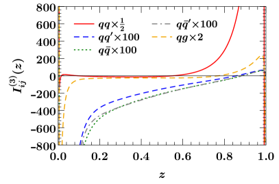
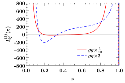
Figure 1: The N³LO boundary term $I^{(3)}_{ij}$ as a function of $z$ in all channels contributing to the quark beam function (left) and the gluon beam function (right). The different channels are rescaled as indicated in the figures.

To illustrate our results, figure 1 shows the beam function boundary terms $I_{ij}(z)$ relevant for the quark beam function (left) and gluon beam function (right) as a function of $z$. For the purpose of this plot, we replace the occurring distributions as $\delta(1-z)\to 0$ and $\mathcal{L}_{n}(1-z)\to\ln^{n}(1-z)/(1-z)$. Since the different channels give rise to very different shapes and magnitudes, they are rescaled as indicated for illustration purposes only.

To study the impact of our calculation on the beam function itself, we consider the cumulative beam function

$$B_{i}(t_{\rm cut},z,\mu)=\int_{0}^{t_{\rm cut}}\mathrm{d}t\,B_{i}(t,z,\mu)=\sum_{j}\int_{z}^{1}\frac{\mathrm{d}z^{\prime}}{z^{\prime}}\int_{0}^{t_{\rm cut}}\mathrm{d}t\,\mathcal{I}_{ij}(t,z^{\prime},\mu)f_{j}\Bigl{(}\frac{z}{z^{\prime}},\mu\Bigr{)}\,,$$ (17)

where we distinguish both quantities only by their arguments. As indicated, this always involves the sum over all flavors $j$ contribution the desired beam function of flavor $i$. We use the MMHT2014nnlo68cl PDF set from ref. Harland-Lang:2014zoa with $\alpha_{s}(m_{Z})=0.118$, and evaluate eq. (17) through an implementation of our results in SCETlib scetlib .

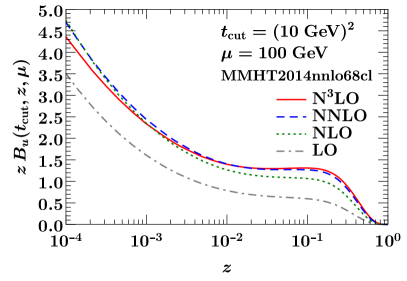
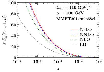
Figure 2: The cumulative $u$-quark (left) and the gluon (right) beam functions as a function of $z$ for fixed $t_{\rm cut}=(10~{}\,\mathrm{GeV})^{2}$ and $\mu=100~{}\,\mathrm{GeV}$. We show the result at LO (which corresponds to the PDF), NLO, NNLO and N³LO.

In figure 2, we compare the $u$-quark beam function (left) and gluon beam function (right) at LO (gray, dot-dashed), NLO (green, dotted), NNLO (blue, dashed) and N³LO (red, solid) as a function of $z$. We fix $t_{\rm cut}=(10~{}\,\mathrm{GeV})^{2}$ and $\mu=100~{}\,\mathrm{GeV}$ and rescale the beam functions by $z$. Note that the LO result corresponds to the PDF itself, and thus illustrates the different shape of the beam function compared to the PDF. While we observe a notable effect of the N³LO corrections, the beam functions show good convergence overall.

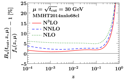
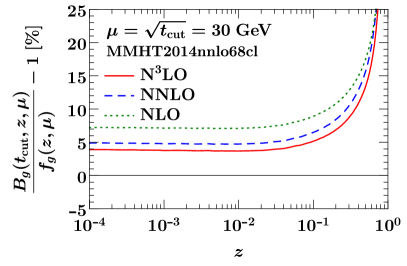
Figure 3: The relative difference of cumulative $u$-quark beam function (left) and the cumulative gluon beam function (right) to the corresponding PDF, as a function. We fix $\mu=\sqrt{t_{\rm cut}}=30~{}\,\mathrm{GeV}$, such that the shown beam function corresponds to the boundary term in a resummed prediction. The different colors show the results at NLO, NNLO and N³LO, respectively.

To judge the impact of the new three-loop boundary term $I_{ij}^{(3)}$ on resummed predictions, it is more useful to show the beam function $B_{i}(t_{\rm cut},z,\mu)$ at its canonical scale $\mu=\sqrt{t_{\rm cut}}$, where all distributions $\mathcal{L}_{m}$ in eq. (3) vanish and only the boundary term $I_{ij}^{(3)}$ contributes. In figure 3, we show the cumulative beam functions at the canonical scale with $\mu=\sqrt{t_{\rm cut}}=30~{}\,\mathrm{GeV}$, showing the relative difference of the $u$-quark beam function (left) and the gluon beam function (right) at NLO (green, dotted), NNLO (blue, dashed) and N³LO (red, solid) to the corresponding PDF itself. We observe that the shape of the beam functions differ significantly from the shape of the PDF for large $z$, but tend to converge towards the PDF for small $z\lesssim 10^{-1}$. As before, we see good convergence at N³LO, but still a notable effect of the N³LO corrections itself.

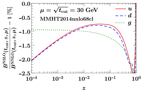
Figure 4: The $K$-factor of the N³LO beam function, i.e. the ratio of the N³LO contribution to the NNLO beam function.We fix $\mu=\sqrt{t_{\rm cut}}=30~{}\,\mathrm{GeV}$, such that the shown beam function corresponds to the boundary term in a resummed prediction. The different colors show the results for an $u$-quark, $d$-quark and gluon, respectively.

Finally, in figure 4 we show the $K$-factor of the N³LO beam function, which we define as the ratio of the N³LO beam to the NNLO beam function. As before, we choose the canonical scales $\mu=\sqrt{t_{\rm cut}}=30~{}\,\mathrm{GeV}$ as relevant for a resummed calculation, We show the $K$ factor for $u$ quarks (red, solid), $d$ quarks (blue, dashed) and gluons (green, dotted). In all cases, we see corrections of $\sim 1-2\%$ with a sizable dependence on $z$.

For completeness, we also show the high-energy limit $z\to 0$ of the kernels $I_{ij}^{(3)}(z)$ in appendix B. This limit is for example interesting because the small-$\mathcal{T}_{1}$ region is known to grow at small $z$ in deep inelastic scattering Kang:2013nha ; Kang:2014qba .

4 Conclusions

We have calculated the perturbative matching kernel relating $N$-jettiness beam functions with lightcone PDFs in all partonic channels for the first time at N³LO in QCD. Our calculation is based on a method recently developed by us to expand hadronic collinear cross sections Ebert:CollExp , demonstrating its usefulness for the calculation of universal ingredients arising in the collinear limit of QCD.

We provide our results in the form of ancillary file with this submission, where we include the renormalized $N$-jettiness beam function in both momentum ($t$) and Fourier ($y$) space. For the $t$ space result, we also provide its expansions around $z=0$ and $z=1$ through 50 orders in the expansion.

In contrast to the TMD beam functions, which are based on the same collinear limit and at N³LO can be entirely expressed in terms of harmonic polylogarithms up to weight 5 Luo:2019szz ; Ebert:PTBF , the $\mathcal{T}_{N}$ beam functions have a much richer structure of the appearing functions and are expressed in terms of Goncharov polylogarithm, as well as iterated integrals with letters that involve square roots. It will be interesting to better understand the source of this difference.

Our results have various phenomenological applications. Firstly, we provide a key ingredient to extend the $N$-jettiness subtraction method Boughezal:2015dva ; Gaunt:2015pea to N³LO, which can be used to obtain exact fully-differential cross sections at this order. They are also crucial to extend the resummation of $\mathcal{T}_{N}$ to N³LL^′ and N⁴LL accuracy, and for matching N³LO calculations to parton showers based on $\mathcal{T}_{0}$ resummation Alioli:2012fc ; Alioli:2015toa .

It will also be interesting to further study the collinear limit of QCD using the underlying method of collinear expansions. In particular, we expect this to shed light on the universal structure of $\mathcal{T}_{N}$ factorization at subleading power Kolodrubetz:2016uim ; Feige:2017zci ; Moult:2017rpl ; Chang:2017atu ; Beneke:2017ztn ; Beneke:2018rbh ; Moult:2018jjd ; Moult:2019mog ; Moult:2019uhz , which has recently attracted much attention in the literature due to its importance for $\mathcal{T}_{N}$-subtractions Moult:2016fqy ; Boughezal:2016zws ; Moult:2017jsg ; Boughezal:2018mvf ; Ebert:2018lzn ; Bhattacharya:2018vph ; Boughezal:2019ggi ; Ebert:2019zkb .

Appendix A Ingredients for the calculation of the beam function

In this appendix, we provide more details on the regularization and renormalization of the beam function kernels. Details of the calculation of all required integrals will be presented in ref. Ebert:ThingsToCome .

A.1 Renormalization group equations

In $t$ space, the beam function $B_{i}(t,z,\mu)$ obeys the RGE Stewart:2009yx ; Stewart:2010qs

$$\mu\frac{\mathrm{d}}{\mathrm{d}\mu}B_{i}(t,z,\mu) =\int\!\mathrm{d}t^{\prime}\,\gamma_{B}^{i}(t-t^{\prime},\mu)\,B_{i}(t^{\prime},z,\mu)\,,$$ (18)

where the anomalous dimension $\gamma_{B}^{i}$ has the all-order form

$$\gamma_{B}^{i}(t,\mu)=-2\Gamma_{\rm cusp}^{i}[\alpha_{s}(\mu)]\,\mathcal{L}_{0}(t,\mu^{2})+\gamma_{B}^{i}[\alpha_{s}(\mu)]\,\delta(t)\,.$$ (19)

Here, $\Gamma_{\rm cusp}^{i}(\alpha_{s})$ and $\gamma^{i}_{B}(\alpha_{s})$ are the cusp and beam noncusp anomalous dimensions, which both depend on the color representation $i=q$ or $i=g$ only, but are independent of the quark flavor. The RGE for the matching kernel follows from eqs. (8) and (18) and the DGLAP equation

$$\mu\frac{\mathrm{d}}{\mathrm{d}\mu}f_{i}(z,\mu)=2\sum_{j}\int_{z}^{1}\!\frac{\mathrm{d}z^{\prime}}{z^{\prime}}\,P_{ij}(z^{\prime},\mu)\,f_{j}\Bigl{(}\frac{z}{z^{\prime}},\mu\Bigr{)}\,.$$ (20)

It is given by Stewart:2010qs

$$\mu\frac{\mathrm{d}}{\mathrm{d}\mu}\mathcal{I}_{ij}(t,z,\mu)=\sum_{k}\int\!\mathrm{d}t^{\prime}\,\int_{z}^{1}\!\frac{\mathrm{d}z^{\prime}}{z^{\prime}}\,\mathcal{I}_{ik}\Bigl{(}t-t^{\prime},\frac{z}{z^{\prime}},\mu\Bigr{)}\Bigl{[}\gamma_{B}^{i}(t^{\prime},\mu)\,\delta_{kj}\delta(1-z^{\prime})-\delta(t^{\prime})\,2P_{kj}(z^{\prime},\mu)\Bigr{]}\,.$$ (21)

A.2 Structure of the beam function counterterm

We define the Fourier transformation of a function $f$ as

$$\tilde{f}(y,\cdots)=\int\mathrm{d}t\,e^{-\mathrm{i}ty}\,f(t,\cdots)\,,\qquad f(t,\cdots)=\int\frac{\mathrm{d}y}{2\pi}\,e^{\mathrm{i}ty}\,\tilde{f}(y,\cdots)\,.$$ (22)

The Fourier transform of the bare kernel $\mathcal{I}_{ij}(t,z,\epsilon)$ can be conveniently evaluated using

$$\mu^{2a\epsilon}\int_{-\infty}^{\infty}\mathrm{d}t\,e^{-\mathrm{i}ty}\frac{\theta(t)}{t^{1+a\epsilon}}=e^{a\epsilon(L_{y}-\gamma_{E})}\Gamma(-a\epsilon)\,,\qquad L_{y}=\ln\bigl{(}\mathrm{i}y\mu^{2}e^{\gamma_{E}}\bigr{)}\,.$$ (23)

Here, $L_{y}$ is the canonical logarithm in Fourier space, and $\gamma_{E}$ is the Euler-Mascheroni constant. In Fourier space, the renormalization of the bare matching kernel in eq. (10) becomes multiplicative in $y$,

$$\tilde{\mathcal{I}}_{ij}(y,z,\mu)=\sum_{k}\int_{z}^{1}\!\frac{\mathrm{d}z^{\prime}}{z^{\prime}}\,\Gamma_{jk}\Bigl{(}\frac{z}{z^{\prime}},\epsilon\Bigr{)}\,\tilde{Z}_{B}^{i}(y,\epsilon,\mu)\hat{Z}_{\alpha_{s}}(\mu,\epsilon)\,\tilde{\mathcal{I}}_{ik}(y,z^{\prime},\epsilon)\,,$$ (24)

and the counterterm $\tilde{Z}_{B}^{i}$ follows from the RG eq. (19) in $y$ space,

$$\frac{\mathrm{d}}{\mathrm{d}\ln\mu}\ln{\tilde{B}_{i}(y,z,\mu)} =\tilde{\gamma}_{B}^{i}(y,\mu)=-\frac{\mathrm{d}}{\mathrm{d}\ln\mu}\ln\tilde{Z}_{B}^{i}(y,\mu,\epsilon)$$

$$=2\Gamma_{\rm cusp}^{i}[\alpha_{s}(\mu)]L_{y}+\gamma_{B}^{i}[\alpha_{s}(\mu)]\,.$$ (25)

Solving eq. (A.2), we can predict the all-order pole structure of $\tilde{Z}_{B}^{i}$ as (see also ref. Becher:2009cu )

$$\ln\tilde{Z}^{B}_{i}(y,\mu,\epsilon)=-\int\limits_{0}^{\alpha_{s}(\mu)}\!\!\frac{\mathrm{d}\alpha}{\beta(\alpha,\epsilon)}\biggl{[}4\Gamma_{\rm cusp}^{i}(\alpha)\int_{\alpha_{s}(\mu)}^{\alpha}\frac{\mathrm{d}\alpha^{\prime}}{\beta(\alpha^{\prime},\epsilon)}+2\Gamma_{\rm cusp}^{i}(\alpha)L_{y}+\gamma_{B}^{i}(\alpha)\biggr{]}\,,$$ (26)

where $\beta(\alpha_{s},\epsilon)=-2\epsilon\alpha_{s}+\beta(\alpha_{s})$ is the QCD beta function in $d=4-2\epsilon$ dimensions. Expanding eq. (26) systematically in $\alpha$, we obtain the result through three loops as

$$\ln\tilde{Z}^{B}_{i}(y,\mu,\epsilon) =\frac{\alpha_{s}}{4\pi}\biggl{\{}\frac{\Gamma_{0}^{i}}{\epsilon^{2}}+\frac{1}{2\epsilon}\bigl{(}2\Gamma_{0}^{i}L_{y}+\gamma_{B\,0}^{i}\bigr{)}\biggr{\}}$$

$$+\Bigl{(}\frac{\alpha_{s}}{4\pi}\Bigr{)}^{2}\biggl{\{}-\frac{3}{4}\frac{\beta_{0}\Gamma_{0}^{i}}{\epsilon^{3}}-\frac{1}{4\epsilon^{2}}\bigl{[}\beta_{0}\bigl{(}2\Gamma_{0}^{i}L_{y}+\gamma_{B\,0}^{i}\bigr{)}-\Gamma_{1}^{i}\bigr{]}+\frac{1}{4\epsilon}\bigl{(}2\Gamma_{1}^{i}L_{y}+\gamma_{B\,1}^{i}\bigr{)}\biggr{\}}$$

$$+\Bigl{(}\frac{\alpha_{s}}{4\pi}\Bigr{)}^{3}\biggl{\{}\frac{11}{18}\frac{\beta_{0}^{2}\Gamma_{0}^{i}}{\epsilon^{4}}+\frac{1}{6\epsilon^{3}}\biggl{[}\beta_{0}^{2}\bigl{(}2\Gamma_{0}^{i}L_{y}+\gamma_{B\,0}^{i}\bigr{)}-\frac{5}{3}\beta_{0}\Gamma_{1}^{i}-\frac{8}{3}\beta_{1}\Gamma_{0}^{i}\biggr{]}$$

$$\hskip 51.21504pt-\frac{1}{6\epsilon^{2}}\biggl{[}\beta_{1}\bigl{(}2\Gamma_{0}^{i}L_{y}+\gamma_{B\,0}^{i}\bigr{)}+\beta_{0}\bigl{(}2\Gamma_{1}^{i}L_{y}+\gamma_{B\,1}^{i}\bigr{)}-\frac{2}{3}\Gamma_{2}^{i}\biggr{]}$$

$$\hskip 51.21504pt+\frac{1}{6\epsilon}\bigl{(}2\Gamma_{2}^{i}L_{y}+\gamma_{B\,2}^{i}\bigr{)}\biggr{\}}+\mathcal{O}(\alpha_{s}^{4})\,.$$ (27)

Here, the $\gamma_{n}$ are the coefficients of the corresponding anomalous dimensions at $\mathcal{O}[(\alpha_{s}/4\pi)^{n}]$. Explicit expressions for all anomalous dimensions in the convention of eq. (A.2) are collected in ref. Billis:2019vxg . The required three-loop results for $\Gamma_{\rm cusp}$ and $\beta$ were calculated in refs. Korchemsky:1987wg ; Moch:2004pa ; Vogt:2004mw and refs. Tarasov:1980au ; Larin:1993tp , respectively. The beam noncusp anomalous dimension were originally determined in refs. Stewart:2010qs ; Berger:2010xi , see also refs. Bruser:2018rad ; Banerjee:2018ozf .

A.3 $\alpha_{s}$ renormalization and IR counterterms

The bare strong coupling constant is renormalised as

$$\alpha_{s}^{b} = \alpha_{s}\left(\frac{\mu^{2}}{4\pi}e^{\gamma_{E}}\right)^{\epsilon}\left[1+\frac{\alpha_{s}}{4\pi}\left(-\frac{\beta_{0}}{\epsilon}\right)+\left(\frac{\alpha_{s}}{4\pi}\right)^{2}\left(\frac{\beta_{0}^{2}}{\epsilon^{2}}-\frac{\beta_{1}}{2\epsilon}\right)\right.$$ (28)

$$\hskip 71.13188pt+\left.\left(\frac{\alpha_{s}}{4\pi}\right)^{3}\left(-\frac{\beta_{0}^{3}}{\epsilon^{3}}+\frac{7\beta_{1}\beta_{0}}{6\epsilon^{2}}-\frac{\beta_{2}}{3\epsilon}\right)+\mathcal{O}(\alpha_{s}^{4})\right]\,.$$

The mass factorisation counter term can be expressed in terms of the splitting functions $P_{ij}$ Moch:2004pa ; Vogt:2004mw as

$$\Gamma_{ij}(z)= \delta_{ij}\delta(1-z)$$ (29)

$$+\left(\frac{\alpha_{s}}{4\pi}\right)\frac{P^{(0)}_{ij}}{\epsilon}$$

$$+\left(\frac{\alpha_{s}}{4\pi}\right)^{2}\left[\frac{1}{2\epsilon^{2}}\left(P^{(0)}_{ik}\otimes P^{(0)}_{kj}-\beta_{0}P^{(0)}_{ij}\right)+\frac{1}{2\epsilon}P^{(1)}_{kj}\right]$$

$$+\left(\frac{\alpha_{s}}{4\pi}\right)^{3}\left[\frac{1}{6\epsilon^{3}}\left(P^{(0)}_{ik}\otimes P^{(0)}_{kl}\otimes P^{(0)}_{lj}-3\beta_{0}P^{(0)}_{ik}\otimes P^{(0)}_{kj}+2\beta_{0}^{2}P^{(0)}_{ij}\right)\right.$$

$$\hskip 45.52458pt\left.+\frac{1}{6\epsilon^{2}}\left(P^{(1)}_{ik}\otimes P^{(0)}_{kj}+2P^{(0)}_{ik}\otimes P^{(1)}_{kj}-2\beta_{0}P^{(1)}_{ij}-2\beta_{1}P^{(0)}_{ij}\right)+\frac{1}{3\epsilon}P^{(2)}_{ij}\right].$$

$$+~{}\mathcal{O}(\alpha_{s}^{4})\,.$$

Here, we suppress the argument $z$ of the splitting functions on the right hand side and keep the summation over repeated flavor indices implicit. The convolution in eq. (29) is defined as

$$f\otimes g=\int_{z}^{1}\frac{\mathrm{d}z^{\prime}}{z^{\prime}}f(z)g\left(\frac{z}{z^{\prime}}\right).$$ (30)

Appendix B High-energy limit of the beam function kernels

Here, we present the high-energy limit $z\to 0$ of the beam function $I_{ij}^{(3)}(z)$:

$$\lim\limits_{z\rightarrow 0}z\,I_{gg}^{(3)}(z) = -\frac{1}{120}C_{A}^{3}\ln^{5}(z)+\ln^{4}(z)\left(\frac{11C_{A}^{3}}{72}-\frac{C_{A}^{2}n_{f}}{72}-\frac{C_{A}C_{F}n_{f}}{72}\right)$$ (31)

$$+ \ln^{3}(z)\left[C_{A}^{3}\left(-\frac{\zeta_{2}}{4}-\frac{229}{216}\right)+\frac{17C_{A}^{2}n_{f}}{54}+C_{A}\left(\frac{C_{F}n_{f}}{6}-\frac{n_{f}^{2}}{108}\right)-\frac{C_{F}n_{f}^{2}}{27}\right]$$

$$+ \ln^{2}(z)\left[C_{A}^{3}\left(\frac{143\zeta_{2}}{16}-\frac{25\zeta_{3}}{24}-\frac{1013}{96}\right)+C_{A}^{2}n_{f}\left(\frac{1207}{432}-\frac{17\zeta_{2}}{24}\right)\right.$$

$$\left.\hskip 28.45274pt+C_{A}\left(C_{F}n_{f}\left(\frac{745}{864}-\frac{3\zeta_{2}}{4}\right)-\frac{23n_{f}^{2}}{216}\right)+C_{F}^{2}n_{f}\left(\frac{11}{48}-\frac{\zeta_{2}}{6}\right)-\frac{5C_{F}n_{f}^{2}}{27}\right]$$

$$+ \ln(z)\left[C_{A}^{3}\left(\frac{15143\zeta_{2}}{432}+\frac{407\zeta_{3}}{36}-\frac{1433\zeta_{4}}{48}-\frac{43393}{2592}\right)+C_{F}n_{f}^{2}\left(\frac{\zeta_{2}}{9}-\frac{25}{81}\right)\right.$$

$$\left.\hskip 28.45274pt+C_{A}C_{F}n_{f}\left(-\frac{377}{216}\zeta_{2}-\frac{22\zeta_{3}}{9}+\frac{5033}{3888}\right)+C_{A}n_{f}^{2}\left(\frac{\zeta_{2}}{18}-\frac{251}{648}\right)\right.$$

$$\left.\hskip 28.45274pt+C_{F}^{2}n_{f}\left(\frac{311}{288}-\frac{25\zeta_{2}}{36}\right)+C_{A}^{2}n_{f}\left(-\frac{1031}{216}\zeta_{2}-\frac{\zeta_{3}}{18}+\frac{11027}{1296}\right)\right]$$

$$+ \mathcal{O}(\ln^{0}z)\,,$$

$$\lim\limits_{z\rightarrow 0}z\,I_{gq}^{(3)}(z) = -\frac{1}{120}C_{A}^{2}C_{F}\ln^{5}(z)+\ln^{4}(z)\left(\frac{5C_{A}^{2}C_{F}}{36}-\frac{C_{A}C_{F}n_{f}}{36}+\frac{C_{F}^{2}n_{f}}{72}\right)$$ (32)

$$+ \ln^{3}(z)\left[C_{A}^{2}C_{F}\left(\frac{\zeta_{2}}{12}-\frac{89}{72}\right)+C_{A}C_{F}^{2}\left(\frac{5}{24}-\frac{\zeta_{2}}{3}\right)\right.$$

$$\left.\hskip 28.45274pt+C_{A}C_{F}n_{f}\frac{97}{216}-\frac{C_{F}^{2}n_{f}}{54}-\frac{C_{F}n_{f}^{2}}{36}\right]$$

$$+ \ln^{2}(z)\left[C_{A}^{2}C_{F}\left(\frac{103\zeta_{2}}{16}-\frac{7\zeta_{3}}{24}-\frac{83}{9}\right)+C_{A}C_{F}^{2}\left(\frac{73\zeta_{2}}{24}-\frac{5\zeta_{3}}{4}-\frac{151}{96}\right)\right.$$

$$\left.\hskip 28.45274pt-\frac{5C_{F}n_{f}^{2}}{36}+C_{A}C_{F}n_{f}\left(\frac{2275}{864}-\frac{2\zeta_{2}}{3}\right)+C_{F}^{3}\left(-\frac{3\zeta_{2}}{4}+\frac{\zeta_{3}}{2}+\frac{13}{16}\right)\right.$$

$$\left.\hskip 28.45274pt+C_{F}^{2}n_{f}\left(\frac{157}{432}-\frac{3\zeta_{2}}{4}\right)\right]$$

$$+ \ln(z)\left[C_{F}^{3}\left(-\frac{19}{8}\zeta_{2}+\frac{3\zeta_{3}}{2}-5\zeta_{4}+\frac{93}{16}\right)+C_{A}C_{F}n_{f}\left(-\frac{265}{108}\zeta_{2}-\frac{\zeta_{3}}{6}+\frac{1619}{324}\right)\right.$$

$$\left.\hskip 28.45274pt+C_{F}^{2}n_{f}\left(-\frac{193}{108}\zeta_{2}-\frac{37\zeta_{3}}{18}+\frac{24757}{7776}\right)\right.$$

$$\left.\hskip 28.45274pt+C_{A}C_{F}^{2}\left(\frac{757\zeta_{2}}{48}-\frac{9\zeta_{3}}{4}-\frac{45\zeta_{4}}{8}-\frac{3055}{192}\right)\right.$$

$$\left.\hskip 28.45274pt+C_{A}^{2}C_{F}\left(\frac{2099\zeta_{2}}{108}+\frac{106\zeta_{3}}{9}-\frac{923\zeta_{4}}{48}-\frac{3377}{576}\right)-\frac{25C_{F}n_{f}^{2}}{108}\right]$$

$$+ \mathcal{O}(\ln^{0}z)\,,$$

$$\lim\limits_{z\rightarrow 0}z\,I_{qg}^{(3)}(z) = C_{A}^{2}\left(\frac{2\zeta_{3}}{9}-\frac{322}{243}\right)\ln(z)$$ (33)

$$+ C_{A}^{2}\left(-\frac{1}{324}337\zeta_{2}+\frac{787\zeta_{3}}{432}+\frac{263\zeta_{4}}{144}-\frac{266675}{23328}\right)+C_{A}n_{f}\left(-\frac{\zeta_{3}}{27}-\frac{1169}{23328}\right)$$

$$+ C_{A}C_{F}\left(-\frac{\zeta_{2}}{108}-\frac{7\zeta_{4}}{6}-\frac{\zeta_{3}}{12}-\frac{1103}{1728}\right)+C_{F}n_{f}\left(\frac{6049}{11664}-\frac{2\zeta_{3}}{27}\right)\,,$$

$$\lim\limits_{z\rightarrow 0}z\,I_{qq}^{(3)}(z) = \lim\limits_{z\rightarrow 0}z\,I_{q\bar{q}}^{(3)}(z)=\lim\limits_{z\rightarrow 0}z\,I_{qq^{\prime}}^{(3)}(z)=\lim\limits_{z\rightarrow 0}z\,I_{q\bar{q}^{\prime}}^{(3)}(z)$$ (34)

$$= C_{A}C_{F}\left(\frac{2\zeta_{3}}{9}-\frac{322}{243}\right)\ln(z)+C_{F}^{2}\left(-\frac{\zeta_{2}}{108}-\frac{7\zeta_{4}}{6}-\frac{\zeta_{3}}{12}-\frac{1103}{1728}\right)$$

$$+ C_{F}n_{f}\left(\frac{305}{1458}-\frac{2\zeta_{3}}{27}\right)+C_{A}C_{F}\left(-\frac{337}{324}\zeta_{2}+\frac{257\zeta_{3}}{144}+\frac{263\zeta_{4}}{144}-\frac{258211}{23328}\right)\!.$$

Here, the color factors $C_{A}$ and $C_{F}$ are only used for compactness of the result and should be replaced with their expressions in terms of $n_{c}$. Note that the expressions for the high energy limit ${z\rightarrow 0}$ up to $\mathcal{O}(z^{50})$, as well as that for the threshold limit $z\to 1$ up to $\mathcal{O}((1-z)^{50})$, can be found in electronic form in the ancillary files.

References

- (1) ATLAS collaboration, M. Aaboud et al., Measurement of the -boson mass in pp collisions at TeV with the ATLAS detector, Eur. Phys. J. C78 (2018) 110 [1701.07240].
- (2) ATLAS collaboration, M. Aaboud et al., Measurement of the Drell-Yan triple-differential cross section in collisions at TeV, JHEP 12 (2017) 059 [1710.05167].
- (3) CMS collaboration, V. Khachatryan et al., Measurement of the transverse momentum spectra of weak vector bosons produced in proton-proton collisions at TeV, JHEP 02 (2017) 096 [1606.05864].
- (4) CMS collaboration, A. M. Sirunyan et al., Measurements of differential Z boson production cross sections in proton-proton collisions at = 13 TeV, JHEP 12 (2019) 061 [1909.04133].
- (5) CMS collaboration, A. M. Sirunyan et al., Combined measurements of Higgs boson couplings in proton–proton collisions at , Eur. Phys. J. C79 (2019) 421 [1809.10733].
- (6) ATLAS collaboration, G. Aad et al., Higgs boson production cross-section measurements and their EFT interpretation in the decay channel at = 13 TeV with the ATLAS detector, 2004.03447.
- (7) ATLAS collaboration, M. Aaboud et al., Measurement of fiducial and differential production cross-sections at TeV with the ATLAS detector, Eur. Phys. J. C79 (2019) 884 [1905.04242].
- (8) ATLAS collaboration, M. Aaboud et al., Measurement of production in the final state with the ATLAS detector in collisions at TeV, JHEP 10 (2019) 127 [1905.07163].
- (9) CMS collaboration, A. M. Sirunyan et al., Search for anomalous triple gauge couplings in WW and WZ production in lepton + jet events in proton-proton collisions at 13 TeV, JHEP 12 (2019) 062 [1907.08354].
- (10) C. Anastasiou, C. Duhr, F. Dulat, E. Furlan, T. Gehrmann, F. Herzog et al., Higgs boson gluon–fusion production at threshold in N3LO QCD, Phys. Lett. B737 (2014) 325 [1403.4616].
- (11) C. Anastasiou, C. Duhr, F. Dulat, F. Herzog and B. Mistlberger, Higgs Boson Gluon-Fusion Production in QCD at Three Loops, Phys. Rev. Lett. 114 (2015) 212001 [1503.06056].
- (12) F. A. Dreyer and A. Karlberg, Vector-Boson Fusion Higgs Production at Three Loops in QCD, Phys. Rev. Lett. 117 (2016) 072001 [1606.00840].
- (13) F. A. Dreyer and A. Karlberg, Vector-Boson Fusion Higgs Pair Production at N3LO, Phys. Rev. D98 (2018) 114016 [1811.07906].
- (14) B. Mistlberger, Higgs boson production at hadron colliders at N3LO in QCD, JHEP 05 (2018) 028 [1802.00833].
- (15) C. Duhr, F. Dulat and B. Mistlberger, Higgs production in bottom-quark fusion to third order in the strong coupling, 1904.09990.
- (16) C. Duhr, F. Dulat, V. Hirschi and B. Mistlberger, Higgs production in bottom quark fusion: Matching the 4- and 5-flavour schemes to third order in the strong coupling, 2004.04752.
- (17) C. Duhr, F. Dulat and B. Mistlberger, The Drell-Yan cross section to third order in the strong coupling constant, 2001.07717.
- (18) L. Cieri, X. Chen, T. Gehrmann, E. W. N. Glover and A. Huss, Higgs boson production at the LHC using the subtraction formalism at N3LO QCD, JHEP 02 (2019) 096 [1807.11501].
- (19) F. Dulat, B. Mistlberger and A. Pelloni, Precision predictions at N3LO for the Higgs boson rapidity distribution at the LHC, Phys. Rev. D99 (2019) 034004 [1810.09462].
- (20) I. W. Stewart, F. J. Tackmann and W. J. Waalewijn, Factorization at the LHC: From PDFs to Initial State Jets, Phys. Rev. D81 (2010) 094035 [0910.0467].
- (21) I. W. Stewart, F. J. Tackmann and W. J. Waalewijn, N-Jettiness: An Inclusive Event Shape to Veto Jets, Phys. Rev. Lett. 105 (2010) 092002 [1004.2489].
- (22) I. W. Stewart, F. J. Tackmann and W. J. Waalewijn, The Beam Thrust Cross Section for Drell-Yan at NNLL Order, Phys. Rev. Lett. 106 (2011) 032001 [1005.4060].
- (23) T. T. Jouttenus, I. W. Stewart, F. J. Tackmann and W. J. Waalewijn, The Soft Function for Exclusive N-Jet Production at Hadron Colliders, Phys. Rev. D83 (2011) 114030 [1102.4344].
- (24) C. W. Bauer, S. Fleming and M. E. Luke, Summing Sudakov logarithms in in effective field theory, Phys. Rev. D63 (2000) 014006 [hep-ph/0005275].
- (25) C. W. Bauer, S. Fleming, D. Pirjol and I. W. Stewart, An Effective field theory for collinear and soft gluons: Heavy to light decays, Phys. Rev. D63 (2001) 114020 [hep-ph/0011336].
- (26) C. W. Bauer and I. W. Stewart, Invariant operators in collinear effective theory, Phys. Lett. B516 (2001) 134 [hep-ph/0107001].
- (27) C. W. Bauer, D. Pirjol and I. W. Stewart, Soft collinear factorization in effective field theory, Phys. Rev. D65 (2002) 054022 [hep-ph/0109045].
- (28) C. W. Bauer, S. Fleming, D. Pirjol, I. Z. Rothstein and I. W. Stewart, Hard scattering factorization from effective field theory, Phys. Rev. D66 (2002) 014017 [hep-ph/0202088].
- (29) G. Lustermans, J. K. L. Michel and F. J. Tackmann, Generalized Threshold Factorization with Full Collinear Dynamics, 1908.00985.
- (30) R. Boughezal, C. Focke, X. Liu and F. Petriello, -boson production in association with a jet at next-to-next-to-leading order in perturbative QCD, Phys. Rev. Lett. 115 (2015) 062002 [1504.02131].
- (31) J. Gaunt, M. Stahlhofen, F. J. Tackmann and J. R. Walsh, N-jettiness Subtractions for NNLO QCD Calculations, JHEP 09 (2015) 058 [1505.04794].
- (32) S. Catani and M. Grazzini, An NNLO subtraction formalism in hadron collisions and its application to Higgs boson production at the LHC, Phys. Rev. Lett. 98 (2007) 222002 [hep-ph/0703012].
- (33) G. Billis, M. A. Ebert, J. K. L. Michel and F. J. Tackmann, A Toolbox for and -Jettiness Subtractions at N3LO, 1909.00811.
- (34) I. Moult, L. Rothen, I. W. Stewart, F. J. Tackmann and H. X. Zhu, Subleading Power Corrections for N-Jettiness Subtractions, Phys. Rev. D95 (2017) 074023 [1612.00450].
- (35) I. Moult, L. Rothen, I. W. Stewart, F. J. Tackmann and H. X. Zhu, N -jettiness subtractions for at subleading power, Phys. Rev. D97 (2018) 014013 [1710.03227].
- (36) M. A. Ebert, I. Moult, I. W. Stewart, F. J. Tackmann, G. Vita and H. X. Zhu, Power Corrections for N-Jettiness Subtractions at , JHEP 12 (2018) 084 [1807.10764].
- (37) R. Boughezal, X. Liu and F. Petriello, Power Corrections in the N-jettiness Subtraction Scheme, JHEP 03 (2017) 160 [1612.02911].
- (38) R. Boughezal, A. Isgrò and F. Petriello, Next-to-leading-logarithmic power corrections for -jettiness subtraction in color-singlet production, Phys. Rev. D97 (2018) 076006 [1802.00456].
- (39) R. Boughezal, A. Isgrò and F. Petriello, Next-to-leading power corrections to jet production in -jettiness subtraction, Phys. Rev. D101 (2020) 016005 [1907.12213].
- (40) M. A. Ebert and F. J. Tackmann, Impact of isolation and fiducial cuts on qT and N-jettiness subtractions, JHEP 03 (2020) 158 [1911.08486].
- (41) S. Alioli, C. W. Bauer, C. J. Berggren, A. Hornig, F. J. Tackmann, C. K. Vermilion et al., Combining Higher-Order Resummation with Multiple NLO Calculations and Parton Showers in GENEVA, JHEP 09 (2013) 120 [1211.7049].
- (42) S. Alioli, C. W. Bauer, C. Berggren, F. J. Tackmann and J. R. Walsh, Drell-Yan production at NNLL’+NNLO matched to parton showers, Phys. Rev. D92 (2015) 094020 [1508.01475].
- (43) I. W. Stewart, F. J. Tackmann and W. J. Waalewijn, The Quark Beam Function at NNLL, JHEP 09 (2010) 005 [1002.2213].
- (44) C. F. Berger, C. Marcantonini, I. W. Stewart, F. J. Tackmann and W. J. Waalewijn, Higgs Production with a Central Jet Veto at NNLL+NNLO, JHEP 04 (2011) 092 [1012.4480].
- (45) J. R. Gaunt, M. Stahlhofen and F. J. Tackmann, The Quark Beam Function at Two Loops, JHEP 04 (2014) 113 [1401.5478].
- (46) J. Gaunt, M. Stahlhofen and F. J. Tackmann, The Gluon Beam Function at Two Loops, JHEP 08 (2014) 020 [1405.1044].
- (47) K. Melnikov, R. Rietkerk, L. Tancredi and C. Wever, Double-real contribution to the quark beam function at N3LO QCD, JHEP 02 (2019) 159 [1809.06300].
- (48) K. Melnikov, R. Rietkerk, L. Tancredi and C. Wever, Triple-real contribution to the quark beam function in QCD at next-to-next-to-next-to-leading order, JHEP 06 (2019) 033 [1904.02433].
- (49) A. Behring, K. Melnikov, R. Rietkerk, L. Tancredi and C. Wever, Quark beam function at next-to-next-to-next-to-leading order in perturbative QCD in the generalized large- approximation, Phys. Rev. D100 (2019) 114034 [1910.10059].
- (50) M. D. Schwartz, Resummation and NLO matching of event shapes with effective field theory, Phys. Rev. D77 (2008) 014026 [0709.2709].
- (51) S. Fleming, A. H. Hoang, S. Mantry and I. W. Stewart, Top Jets in the Peak Region: Factorization Analysis with NLL Resummation, Phys. Rev. D77 (2008) 114003 [0711.2079].
- (52) R. Kelley, M. D. Schwartz, R. M. Schabinger and H. X. Zhu, The two-loop hemisphere soft function, Phys. Rev. D84 (2011) 045022 [1105.3676].
- (53) P. F. Monni, T. Gehrmann and G. Luisoni, Two-Loop Soft Corrections and Resummation of the Thrust Distribution in the Dijet Region, JHEP 08 (2011) 010 [1105.4560].
- (54) A. Hornig, C. Lee, I. W. Stewart, J. R. Walsh and S. Zuberi, Non-global Structure of the Dijet Soft Function, JHEP 08 (2011) 054 [1105.4628].
- (55) R. Boughezal, X. Liu and F. Petriello, -jettiness soft function at next-to-next-to-leading order, Phys. Rev. D 91 (2015) 094035 [1504.02540].
- (56) J. M. Campbell, R. K. Ellis, R. Mondini and C. Williams, The NNLO QCD soft function for 1-jettiness, Eur. Phys. J. C 78 (2018) 234 [1711.09984].
- (57) S. Jin and X. Liu, Two-loop -jettiness soft function for production, Phys. Rev. D 99 (2019) 114017 [1901.10935].
- (58) C. W. Bauer and A. V. Manohar, Shape function effects in B —¿ X(s) gamma and B —¿ X(u) l anti-nu decays, Phys. Rev. D 70 (2004) 034024 [hep-ph/0312109].
- (59) T. Becher and M. Neubert, Toward a NNLO calculation of the anti-B —¿ X(s) gamma decay rate with a cut on photon energy. II. Two-loop result for the jet function, Phys. Lett. B 637 (2006) 251 [hep-ph/0603140].
- (60) S. Fleming, A. K. Leibovich and T. Mehen, Resumming the color octet contribution to + , Phys. Rev. D 68 (2003) 094011 [hep-ph/0306139].
- (61) T. Becher and M. D. Schwartz, Direct photon production with effective field theory, JHEP 02 (2010) 040 [0911.0681].
- (62) T. Becher and G. Bell, The gluon jet function at two-loop order, Phys. Lett. B 695 (2011) 252 [1008.1936].
- (63) R. Brüser, Z. L. Liu and M. Stahlhofen, Three-Loop Quark Jet Function, Phys. Rev. Lett. 121 (2018) 072003 [1804.09722].
- (64) P. Banerjee, P. K. Dhani and V. Ravindran, Gluon jet function at three loops in QCD, Phys. Rev. D98 (2018) 094016 [1805.02637].
- (65) M. A. Ebert, B. Mistlberger and G. Vita, Collinear expansion for color singlet cross sections, MIT-CTP 5207 (companion paper) .
- (66) C. Anastasiou and K. Melnikov, Pseudoscalar Higgs boson production at hadron colliders in next-to-next-to-leading order QCD, Physical Review D 67 (2003) 037501.
- (67) C. Anastasiou, L. Dixon and K. Melnikov, NLO Higgs boson rapidity distributions at hadron colliders, Nuclear Physics B - Proceedings Supplements 116 (2003) 193.
- (68) C. Anastasiou, L. Dixon, K. Melnikov and F. Petriello, Dilepton Rapidity Distribution in the Drell-Yan Process at Next-to-Next-to-Leading Order in QCD, Physical Review Letters 91 (2003) 182002.
- (69) C. Anastasiou, K. Melnikov and F. Petriello, Fully differential Higgs boson production and the di-photon signal through next-to-next-to-leading order, Nuclear Physics B 724 (2005) 197.
- (70) C. Anastasiou, L. Dixon, K. Melnikov and F. Petriello, High-precision QCD at hadron colliders: Electroweak gauge boson rapidity distributions at next-to-next-to leading order, Physical Review D 69 (2004) 094008.
- (71) K. Chetyrkin and F. Tkachov, Integration by Parts: The Algorithm to Calculate beta Functions in 4 Loops, Nucl.Phys. B192 (1981) 159.
- (72) F. V. Tkachov, A Theorem on Analytical Calculability of Four Loop Renormalization Group Functions, Phys. Lett. B100 (1981) 65.
- (73) A. Kotikov, Differential equations method: New technique for massive Feynman diagrams calculation, Phys. Lett. B 254 (1991) 158.
- (74) A. Kotikov, Differential equations method: The Calculation of vertex type Feynman diagrams, Phys. Lett. B 259 (1991) 314.
- (75) A. Kotikov, Differential equation method: The Calculation of N point Feynman diagrams, Phys. Lett. B 267 (1991) 123.
- (76) J. M. Henn, Multiloop integrals in dimensional regularization made simple, Phys. Rev. Lett. 110 (2013) 251601 [1304.1806].
- (77) T. Gehrmann and E. Remiddi, Differential equations for two loop four point functions, Nucl. Phys. B580 (2000) 485 [hep-ph/9912329].
- (78) T. Inami, T. Kubota and Y. Okada, Effective Gauge Theory and the Effect of Heavy Quarks, Zeitschrift für Physik C 18 (1983) 69.
- (79) M. Shifman, A. Vainshtein and V. Zakharov, Remarks on Higgs-boson interactions with nucleons, Physics Letters B 78 (1978) 443.
- (80) V. P. Spiridonov and K. G. Chetyrkin, Nonleading mass corrections and renormalization of the operators m psi-bar psi and g**2(mu nu), Sov. J. Nucl. Phys. 47 (1988) 522.
- (81) F. Wilczek, Decays of Heavy Vector Mesons into Higgs Particles, Physical Review Letters 39 (1977) 1304.
- (82) K. G. Chetyrkin, B. A. Kniehl and M. Steinhauser, Decoupling relations to and their connection to low-energy theorems, Nucl. Phys. B510 (1998) 61 [hep-ph/9708255].
- (83) Y. Schroder and M. Steinhauser, Four-loop decoupling relations for the strong coupling, JHEP 01 (2006) 051 [hep-ph/0512058].
- (84) K. Chetyrkin, J. Kühn and C. Sturm, QCD decoupling at four loops, Nuclear Physics B 744 (2006) 121.
- (85) M. Kramer, E. Laenen and M. Spira, Soft gluon radiation in Higgs boson production at the LHC, Nucl. Phys. B511 (1998) 523 [hep-ph/9611272].
- (86) F. Dulat and B. Mistlberger, Real-Virtual-Virtual contributions to the inclusive Higgs cross section at N3LO, 1411.3586.
- (87) F. Dulat, S. Lionetti, B. Mistlberger, A. Pelloni and C. Specchia, Higgs-differential cross section at NNLO in dimensional regularisation, JHEP 07 (2017) 017 [1704.08220].
- (88) F. Dulat, B. Mistlberger and A. Pelloni, Differential Higgs production at N3LO beyond threshold, JHEP 01 (2018) 145 [1710.03016].
- (89) C. Anastasiou, C. Duhr, F. Dulat, F. Herzog and B. Mistlberger, Real-virtual contributions to the inclusive Higgs cross-section at , JHEP 12 (2013) 088 [1311.1425].
- (90) C. Duhr, T. Gehrmann and M. Jaquier, Two-loop splitting amplitudes and the single-real contribution to inclusive Higgs production at N3LO, JHEP 02 (2015) 077 [1411.3587].
- (91) C. Duhr and T. Gehrmann, The two-loop soft current in dimensional regularization, Phys. Lett. B727 (2013) 452 [1309.4393].
- (92) P. Nogueira, Automatic feynman graph generation, Journal of Computational Physics 105 (1993) 279.
- (93) C. Anastasiou, C. Duhr, F. Dulat and B. Mistlberger, Soft triple-real radiation for Higgs production at N3LO, JHEP 07 (2013) 003 [1302.4379].
- (94) C. Anastasiou, C. Duhr, F. Dulat, E. Furlan, T. Gehrmann, F. Herzog et al., Higgs Boson GluonFfusion Production Beyond Threshold in N QCD, JHEP 03 (2015) 091 [1411.3584].
- (95) C. Anastasiou, C. Duhr, F. Dulat, E. Furlan, F. Herzog and B. Mistlberger, Soft expansion of double-real-virtual corrections to Higgs production at N3LO, JHEP 08 (2015) 051 [1505.04110].
- (96) M. A. Ebert, B. Mistlberger and G. Vita, Transverse momentum dependent PDFs at N3LO, MIT-CTP 5209 (companion paper) .
- (97) M. A. Ebert, B. Mistlberger and G. Vita, Calculation of Differential Collinear Expansions at N3LO, (in preparation) .
- (98) E. Remiddi and J. A. M. Vermaseren, Harmonic polylogarithms, Int. J. Mod. Phys. A15 (2000) 725 [hep-ph/9905237].
- (99) A. Goncharov, Multiple polylogarithms and mixed Tate motives, math/0103059.
- (100) C. Duhr, H. Gangl and J. R. Rhodes, From polygons and symbols to polylogarithmic functions, JHEP 10 (2012) 075 [1110.0458].
- (101) C. Duhr, Hopf algebras, coproducts and symbols: an application to Higgs boson amplitudes, JHEP 08 (2012) 043 [1203.0454].
- (102) C. Duhr and F. Dulat, PolyLogTools — polylogs for the masses, JHEP 08 (2019) 135 [1904.07279].
- (103) E. Panzer, Algorithms for the symbolic integration of hyperlogarithms with applications to Feynman integrals, Comput. Phys. Commun. 188 (2015) 148 [1403.3385].
- (104) M. A. Ebert and F. J. Tackmann, Resummation of Transverse Momentum Distributions in Distribution Space, JHEP 02 (2017) 110 [1611.08610].
- (105) L. A. Harland-Lang, A. D. Martin, P. Motylinski and R. S. Thorne, Parton distributions in the LHC era: MMHT 2014 PDFs, Eur. Phys. J. C75 (2015) 204 [1412.3989].
- (106) M. A. Ebert, J. K. L. Michel, F. J. Tackmann et al., SCETlib: A C++ Package for Numerical Calculations in QCD and Soft-Collinear Effective Theory, DESY-17-099 (2018) .
- (107) D. Kang, C. Lee and I. W. Stewart, Using 1-Jettiness to Measure 2 Jets in DIS 3 Ways, Phys. Rev. D88 (2013) 054004 [1303.6952].
- (108) D. Kang, C. Lee and I. W. Stewart, Analytic calculation of 1-jettiness in DIS at , JHEP 11 (2014) 132 [1407.6706].
- (109) M.-x. Luo, T.-Z. Yang, H. X. Zhu and Y. J. Zhu, Quark Transverse Parton Distribution at the Next-to-Next-to-Next-to-Leading Order, Phys. Rev. Lett. 124 (2020) 092001 [1912.05778].
- (110) D. W. Kolodrubetz, I. Moult and I. W. Stewart, Building Blocks for Subleading Helicity Operators, JHEP 05 (2016) 139 [1601.02607].
- (111) I. Feige, D. W. Kolodrubetz, I. Moult and I. W. Stewart, A Complete Basis of Helicity Operators for Subleading Factorization, JHEP 11 (2017) 142 [1703.03411].
- (112) I. Moult, I. W. Stewart and G. Vita, A subleading operator basis and matching for gg -¿ H, JHEP 07 (2017) 067 [1703.03408].
- (113) C.-H. Chang, I. W. Stewart and G. Vita, A Subleading Power Operator Basis for the Scalar Quark Current, JHEP 04 (2018) 041 [1712.04343].
- (114) M. Beneke, M. Garny, R. Szafron and J. Wang, Anomalous dimension of subleading-power N-jet operators, JHEP 03 (2018) 001 [1712.04416].
- (115) M. Beneke, M. Garny, R. Szafron and J. Wang, Anomalous dimension of subleading-power -jet operators. Part II, JHEP 11 (2018) 112 [1808.04742].
- (116) I. Moult, I. W. Stewart, G. Vita and H. X. Zhu, First Subleading Power Resummation for Event Shapes, JHEP 08 (2018) 013 [1804.04665].
- (117) I. Moult, I. W. Stewart and G. Vita, Subleading Power Factorization with Radiative Functions, JHEP 11 (2019) 153 [1905.07411].
- (118) I. Moult, I. W. Stewart, G. Vita and H. X. Zhu, The Soft Quark Sudakov, JHEP 05 (2020) 089 [1910.14038].
- (119) A. Bhattacharya, I. Moult, I. W. Stewart and G. Vita, Helicity Methods for High Multiplicity Subleading Soft and Collinear Limits, JHEP 05 (2019) 192 [1812.06950].
- (120) T. Becher and M. Neubert, Infrared singularities of scattering amplitudes in perturbative QCD, Phys. Rev. Lett. 102 (2009) 162001 [0901.0722].
- (121) G. P. Korchemsky and A. V. Radyushkin, Renormalization of the Wilson Loops Beyond the Leading Order, Nucl. Phys. B283 (1987) 342.
- (122) S. Moch, J. A. M. Vermaseren and A. Vogt, The Three loop splitting functions in QCD: The Nonsinglet case, Nucl. Phys. B688 (2004) 101 [hep-ph/0403192].
- (123) A. Vogt, S. Moch and J. A. M. Vermaseren, The Three-loop splitting functions in QCD: The Singlet case, Nucl. Phys. B691 (2004) 129 [hep-ph/0404111].
- (124) O. V. Tarasov, A. A. Vladimirov and A. Yu. Zharkov, The Gell-Mann-Low Function of QCD in the Three Loop Approximation, Phys. Lett. 93B (1980) 429.
- (125) S. A. Larin and J. A. M. Vermaseren, The Three loop QCD Beta function and anomalous dimensions, Phys. Lett. B303 (1993) 334 [hep-ph/9302208].