Polarized electron-deuteron deep-inelastic scattering with spectator nucleon tagging

Abstract

Background

DIS on the polarized deuteron with detection of a proton in the nuclear breakup region (spectator tagging) represents a unique method for extracting the neutron spin structure functions and studying nuclear modifications. The tagged proton momentum controls the nuclear configuration during the DIS process and enables a differential analysis of nuclear effects. Such measurements could be performed with the future electron-ion collider (EIC) and forward proton detectors if deuteron beam polarization could be achieved.

Purpose

Develop theoretical framework for polarized deuteron DIS with spectator tagging. Formulate procedures for neutron spin structure extraction.

Methods

A covariant spin density matrix formalism is used to describe general deuteron polarization in collider experiments (vector/tensor, pure/mixed). Light-front (LF) quantum mechanics is employed to factorize nuclear and nucleonic structure in the DIS process. A 4-dimensional representation of LF spin structure is used to construct the polarized deuteron LF wave function and efficiently evaluate the spin sums. Free neutron structure is extracted using the impulse approximation and analyticity in the tagged proton momentum (pole extrapolation).

Results

General expressions of the polarized tagged DIS observables in collider experiments. Analytic and numerical study of the polarized deuteron LF spectral function and nucleon momentum distributions. Practical procedures for neutron spin structure extraction from the tagged deuteron spin asymmetries.

Conclusions

Spectator tagging provides new tools for precise neutron spin structure measurements. D-wave depolarization and nuclear binding effects can be eliminated through the tagged proton momentum dependence. The methods can be extended to tensor-polarized observables, spin-orbit effects, and diffractive processes.

I Introduction

Exploring the spin-dependent partonic structure of the nucleon and the numerous polarization-induced phenomena in QCD processes is a principal objective of modern nuclear physics; see Refs. Anselmino et al. (1995); Burkardt et al. (2010); Kuhn et al. (2009); Aidala et al. (2013) for a review. This program requires measurements of deep-inelastic lepton scattering (DIS) on both the proton and the neutron. Proton and neutron data are needed to separate the isovector and isoscalar combinations of the nucleon spin structure functions, which are subject to different short–distance dynamics (QCD evolution, higher–twist effects, small–$x$ asymptotics) and give access to different combinations of the parton densities (non-singlet quarks vs. gluons and singlet quarks) de Florian et al. (2009); Leader et al. (2010); Blumlein and Bottcher (2010); Nocera et al. (2014); Sato et al. (2016).

The isovector structure function $g_{1p}-g_{1n}$ exhibits pure non-singlet QCD evolution and provides direct access to the flavor-nonsinglet polarized quark densities. Its moment (integral over $x$) can be used for precision studies of perturbative QCD and extraction of the strong coupling constant, see Refs. Altarelli et al. (1997); Pasechnik et al. (2010); Baikov et al. (2010); Deur et al. (2014); Cvetič and Kataev (2016); Kotlorz and Mikhailov (2019); Ayala et al. (2018); Deur et al. (2016) and references therein, and is asymptotically constrained by the Bjorken sum rule, a fundamental prediction of current algebra that can be tested experimentally Bjorken (1970). The isoscalar structure function $g_{1p}+g_{1n}$ exhibits singlet evolution and can be used to extract the polarized gluon density and the flavor-singlet polarized quark densities. Both isospin combinations are needed to determine the flavor decomposition of the polarized quark densities and their contributions to the nucleon spin; see Refs. de Florian et al. (2009); Leader et al. (2010); Blumlein and Bottcher (2010); Nocera et al. (2014); Sato et al. (2016) and references therein. The subasymptotic power corrections to the spin structure functions give access to higher-twist matrix elements describing non-perturbative quark-gluon correlations in the nucleon, for which theoretical calculations predict a significant isospin dependence Braun and Kolesnichenko (1987); Balitsky et al. (1990); Stein et al. (1995); Balla et al. (1998), consistent with empirical extractions Meziani et al. (2005); Sidorov and Weiss (2006). Neutron and proton data together are also needed to explore the dynamical mechanisms causing single-spin asymmetries in semi-inclusive DIS, where there are signs of large isovector structures, see Refs. Anselmino et al. (2010, 2014) and references therein.

Neutron spin structure functions are measured in DIS on polarized light nuclei, principally the deuteron $d\equiv{}^{2}$H and ³He. Experiments have been performed at SLAC Anthony et al. (1996); Abe et al. (1998, 1997a, 1997b); Anthony et al. (1999a, b, 2000, 2003) , DESY HERMES Ackerstaff et al. (1997); Airapetian et al. (2007), CERN SMC Adeva et al. (1998), CERN COMPASS Alexakhin et al. (2007); Alekseev et al. (2009); Adolph et al. (2017) and JLab 6 GeV Deur et al. (2014); Zheng et al. (2004); Posik et al. (2014); Prok et al. (2014); Chen et al. (2011), and will be extended further with the JLab 12 GeV Upgrade Malace et al. (2014). The extraction of the neutron structure functions from the nuclear DIS data faces considerable theoretical challenges; see Frankfurt and Strikman (1988); Arneodo (1994); Ciofi degli Atti et al. (1993); Melnitchouk et al. (1995); Kulagin et al. (1995); Piller et al. (1996); Frankfurt et al. (1996); Bissey et al. (2002); Ethier and Melnitchouk (2013) and references therein. The DIS process can happen on the protons or neutrons in the nucleus, causing dilution of the neutron signal. Spin depolarization occurs due to higher partial waves in the nuclear wave function. Nuclear binding modifies the apparent neutron structure functions through the Fermi motion and dynamical effects (EMC effect at $x>0.3$; antishadowing at $x\sim 0.1$; nuclear shadowing at $x<0.01$). These modifications reveal different aspects of nucleon interactions in QCD and are themselves objects of study. In spin structure measurements with polarized ³He, the presence of $\Delta$ isobars in the nuclear wave function (non-nucleonic degrees of freedom) Frankfurt et al. (1996); Bissey et al. (2002) modifies the effective neutron polarization compared to non-relativistic nuclear structure calculations Friar et al. (1990); Ciofi degli Atti et al. (1993).

The main difficulty in the theoretical treatment of the nuclear modifications lies in the fact that they strongly depend on the nuclear configurations present during the DIS process. Both the state of motion and the strength of interaction of the active nucleon depend on the configuration and exhibit considerable variation, as determined by the quantum-mechanical motion of the interacting system. In inclusive measurements one attempts to account for these effects by modeling their dependence on the nuclear configuration and summing over all configurations. The resulting theoretical uncertainty represents a significant source of the systematic error in neutron spin structure function extraction. Efforts should be made to reduce this theoretical uncertainty as the experimental data are becoming more precise. Another strategy is to consider alternative measurements that permit control of the nuclear configuration during the DIS process.

DIS on the deuteron with detection of a proton in the nuclear fragmentation region, $e+d\rightarrow e^{\prime}+X+p$, represents a unique method for performing neutron structure measurements in controlled nuclear configurations Frankfurt and Strikman (1981). The proton is detected with momenta $p_{p}\lesssim$ 300 MeV in the deuteron rest frame. At such momenta the deuteron can be described with good accuracy in terms of nucleonic degrees of freedom ($pn$), and its wave function in nucleonic degrees of freedom is known well both in non-relativistic and in LF quantum mechanics (see below). Configurations with $\Delta$ isobars are suppressed in the isospin-0 system Frankfurt and Strikman (1981). The detection of the proton identifies DIS events with active neutron and eliminates dilution. The measurement of the proton momentum controls the nuclear configuration during the DIS process and enables a differential treatment of nuclear effects. By extrapolating the proton momentum dependence to the unphysical region one can reach $pn$ configurations where the neutron is effectively free, and nuclear binding effects and final-state interactions disappear, which makes possible the extraction of free neutron structure (pole extrapolation, or on-shell extrapolation) Sargsian and Strikman (2006). The technique is theoretically appealing and practically feasible. If it could be applied to polarized electron-deuteron scattering with proton tagging, one could use it to extract the free neutron spin structure function.

Measurements of DIS on the deuteron with proton tagging have been performed in fixed-target experiments at JLab with 6 GeV beam energy with the CLAS spectrometer and the BoNuS proton detector Baillie et al. (2012); Tkachenko et al. (2014). The data provide constraints on the $F_{2n}/F_{2d}$ structure function ratio and the $d/u$ quark density ratio at large $x$. The measurements will be extended to 11 GeV energy with the BoNuS and ALERT detectors Bueltmann et al. ; Armstrong et al. (2017). The BoNuS setup detects only protons with momenta $p_{p}\gtrsim$ 70 MeV, as slower protons cannot escape the target; the measurements therefore use only a small part of the deuteron momentum distribution and preclude accurate on-shell extrapolation. The setup is also limited to unpolarized targets. Other DIS experiments with proton and neutron tagging at larger momenta $p_{p,n}\sim$ few 100 MeV explore the EMC effect and its connection with nucleon short-range correlations Klimenko et al. (2006); Hen et al. (2015, 2014).

The future Electron-Ion Collider (EIC) at BNL will greatly expand the capabilities for DIS measurements on the proton and on light and heavy ions Boer et al. (2011); Accardi et al. (2016). The proposed design will enable electron-proton collisions at center-of-mass (CM) energies $\sqrt{s_{ep}}\sim$ 20–140 GeV and luminosities $\sim 10^{33}$–$10^{34}$ cm^-2 s^-1, and electron-deuteron collisions at electron-nucleon CM energies $\sqrt{s_{eN}}\sim$ 20–100 GeV and similar luminosities per nucleon Aschenauer et al. (2014); Beebe-Wang et al. . In DIS on the deuteron at the collider, the spectator nucleon moves forward with approximately half the deuteron beam momentum and can be detected with forward detectors integrated into the interaction region. The development and integration of such forward detectors have been a priority of the machine design effort and have made major progress. The current conceptual design includes a magnetic dipole spectrometer with multiple active elements for forward proton detection, and a zero-degree calorimeter for forward neutron detection. The apparatus can detect protons with transverse momenta from zero to $\sim$ few 100 MeV with a resolution $\lesssim 30$ MeV, and longitudinal momenta from $\sim 0.5$–$1.5$ times the nominal spectator momentum; for details and neutron detection see Ref. Jentsch . The EIC thus provides excellent capabilities for deuteron DIS with proton tagging. The collider offers many advantages over the fixed-target setup: protons can be detected down to zero momentum in the deuteron rest frame; the magnetic spectrometer provides good momentum resolution; and tagged measurements can be performed with polarized deuteron beams.

Polarization of the deuteron beams in the EIC is regarded as technically possible and considered as a future option Beebe-Wang et al. . Maintaining deuteron polarization in a storage ring is more challenging than proton polarization, as the small magnetic moment of the deuteron renders spin manipulation more difficult. Possibilities for realizing deuteron polarization in the EIC circular storage ring are under investigation; see e.g. Ref. Higinbotham . (A unique solution to the problem of deuteron polarization is a figure-8 layout of the ion ring that compensates the spin precession within one turn, as was proposed in an earlier alternative EIC design Abeyratne et al. (2012).) Together with the forward detection capabilities, deuteron polarization raises the prospect of using polarized deuteron DIS with proton tagging for precision measurements of neutron spin structure at EIC. The setup could also be used for measurements of bound proton spin structure with neutron tagging, of spin-dependent diffractive processes on the deuteron with proton and neutron tagging, and of tensor-polarized deuteron structure. The physics potential such measurements at EIC has been explored in an R&D project Weiss et al. ; Guzey et al. (2014); Cosyn et al. (2014).

In this article we develop the theoretical framework for DIS on the polarized deuteron with spectator tagging. The development proceeds in three steps. In the first step, we derive the general expressions of the differential cross section of polarized electron-deuteron DIS with spectator tagging for the case of arbitrary deuteron polarization (vector and tensor), including the spin asymmetry observables corresponding to specific polarization states in colliding-beam experiments (depolarization factors). In the second step we separate the high-energy DIS process from the low-energy nuclear structure using methods of light-front quantization, calculate the deuteron structure elements entering in the description of tagged DIS in the impulse approximation (IA), and study their properties (limiting cases, sum rules). In the third step we evaluate the longitudinal spin asymmetries in polarized tagged DIS, study their dependence on the tagged proton momentum analytically and numerically, and formulate the procedures for neutron spin structure extraction, including pole extrapolation. We find that the neutron spin structure function $g_{1n}$ can be extracted efficiently from the tagged longitudinal spin asymmetry formed with the deuteron’s $\pm 1$ spin states only (without the $0$ state, involving effective tensor polarization). We comment on possible extensions of the methods to the study of tensor-polarized observables, spin-orbit effects in deuteron breakup, and exclusive scattering processes. Many of the applications considered here were originally discussed in the work of Ref. Frankfurt and Strikman (1983). Some preliminary results of our study were reported earlier in Ref. Cosyn and Weiss (2019).

Our theoretical treatment of deuteron structure in tagged DIS employs the methods of LF quantization of nuclear systems developed in Refs. Frankfurt and Strikman (1981, 1988) and summarized in Ref. Strikman and Weiss (2018) (for a general review of LF quantization, see Refs. Coester (1992); Brodsky et al. (1998); Heinzl (1998)). High-energy processes such as DIS probe the nucleus at fixed LF time $x^{+}=x^{0}+x^{3}$. A description of the nucleus in terms of nucleonic degrees of freedom at fixed $x^{+}$ permits a smooth matching of nuclear and nucleonic structure, preserves the partonic sum rules for the nucleus (baryon number, LF momentum, spin), and exhibits a close correspondence with nonrelativistic nuclear structure. The LF wave function of the deuteron in nucleon degrees of freedom can be obtained by solving the dynamical equation with realistic $NN$ interactions or constructed approximately from the nonrelativistic wave function. The deuteron and nucleon spin states are introduced as LF helicity states, or boost-invariant extensions of the rest-frame spin states, and the deuteron LF spin structure is obtained in direct analogy to the nonrelativistic system (S and D waves). In the traditional “3-dimensional” formulation of LF spin structure one describes the nucleons by LF 2-spinors that are related to the canonical 2-spinors by the Melosh rotation, and constructs the deuteron LF wave function from the 3-dimensional wave function in the center-of-mass frame. In the present work we employ a “4-dimensional” formulation Kondratyuk and Strikman (1984); Frankfurt and Strikman (1983), in which the nucleons are described by LF bispinors and the coupling to the deuteron is implemented through a 4-dimensional vertex function (the equivalence of the two formulations is demonstrated in Appendix B). It permits efficient evaluation of the sums over the nucleon LF helicities and leads to LF formulas in close analogy with those of relativistically covariant quantum field theory (Feynman diagrams). In particular, in the 4-dimensional formulation the effective polarization of the neutron in the deuteron (at a given LF momentum) can be described by a spin density matrix of the same form as that in covariant field theory, with the entire deuteron structure information condensed in an axial 4-vector (polarization vector).

The article is organized as follows. In Sec. II we review the formalism of relativistic spin density matrices of the spin-1/2 and spin-1 system, which will be used throughout this work. In Sec. III we present the general expressions of the cross section and structure functions of tagged DIS on the polarized deuteron with vector and tensor polarization, including the spin asymmetries measured in colliding-beam experiments. We express the kinematic factors (effective polarizations, depolarization factors) in manifestly relativistically invariant form as suitable for colliding-beam experiments. In Sec. IV we summarize the elements of LF quantization and describe the deuteron LF wave function in the 4-dimensional formulation of the spin structure, including its correspondence with the nonrelativistic wave function. In Sec. V we develop the formalism for the evaluation of nucleon one-body operators in the polarized deuteron at fixed LF momentum of the spectator. We derive the effective spin density matrix of the neutron, calculate the LF momentum distribution of the neutron in the polarized deuteron, and study its momentum and spin dependence. In Sec. VI we calculate the polarized tagged DIS cross section and the spin asymmetries in the IA, separating nuclear and nucleonic structure, and study the dependence on the tagged proton momentum. In Sec. VII we study the analytic properties in the tagged proton momentum and discuss the strategies for neutron spin structure extraction through pole extrapolation. In Sec. VIII we summarize the methodological and practical results and discuss possible extensions of the methods to other scattering processes and to nuclei with $A>2$. Appendix A summarizes the definition and properties of the LF helicity spinors used in the calculations. Appendix B describes the 3-dimensional formulation of the deuteron spin structure in LF quantization and demonstrates the equivalence to the 4-dimensional formulation used in the calculations.

Some explanations are in order regarding the limitations of the present study. In the polarized tagged DIS cross section we consider only the structures after integration over the azimuthal angle of the proton (in the frame where the deuteron and the virtual photon momenta are collinear); these structures correspond to those measured in “untagged” DIS and are used for neutron spin structure function extraction. When the azimuthal angle dependence is included, the number of independent structures in the polarized tagged DIS cross section for the spin-1 target becomes very considerable, especially in the case of tensor polarization; this case will be considered in a separate study Cosyn and Weiss (2020).

In the treatment of nuclear structure effects we limit ourselves to the IA, which is sufficient for studying the tagged spin asymmetries used for neutron structure extraction and their analytic properties at small proton momenta. FSI in unpolarized tagged DIS at intermediate $x$ ($\sim$ 0.1–0.5) were calculated in Ref. Strikman and Weiss (2018) and found to be moderate at proton momenta $\lesssim$100 MeV (in the deuteron rest frame); the calculations could be extended to the polarized case. In the practical applications we consider the leading-twist longitudinal spin asymmetries used for tagged measurements of the neutron spin structure function $g_{1n}$; our general expressions cover also the power-suppressed transverse spin asymmetry and the contributions of $g_{2n}$, and the IA calculations could easily be extended to these observables.

II Spin density matrices

II.1 Spin-1/2 particle

We begin by reviewing the formalism of spin density matrices for ensembles of spin states (mixed polarization states) of spin-1/2 and spin-1 particles. We focus on the relativistically covariant representation of the density matrices in terms of 4-vectors and tensors, which will be used throughout the subsequent calculations.

Consider a relativistic spin-1/2 particle with spin states labeled by the quantum number $\lambda=\pm\frac{1}{2}$; the exact definition of the spin states is not needed here and will be specified later. An ensemble of spin states is described by the density matrix in spin quantum numbers,

$$\rho(\lambda,\lambda^{\prime}),\hskip 20.00003pt\sum_{\lambda}\rho(\lambda,\lambda)=1.$$ (1)

Each spin state of the particle corresponds to a bispinor wave function $u(p,\lambda)$, normalized such that $\bar{u}u=2m$, where $p$ is the 4-momentum and $m$ the mass. The spin density matrix in bispinor representation is defined as

$$\rho\;\equiv\;\sum_{\lambda,\lambda^{\prime}}\rho(\lambda,\lambda^{\prime})\;u(p,\lambda)\bar{u}(p,\lambda^{\prime}),\hskip 20.00003pt\textrm{tr}[\rho]\;=\;2m.$$ (2)

A general spin observable is given by a matrix in spin quantum numbers $O(\lambda^{\prime},\lambda)$. In the bispinor representation it corresponds to a bilinear form

$$O(\lambda^{\prime},\lambda)\;\equiv\;\bar{u}(\lambda^{\prime},p)\Gamma u(\lambda,p),$$ (3)

where the specific form of the matrix $\Gamma$ depends on the observable. The expectation value of the observable in the spin ensemble is then obtained as

$$\langle O\rangle\;\equiv\;\sum_{\lambda,\lambda^{\prime}}\rho(\lambda,\lambda^{\prime})O(\lambda^{\prime},\lambda)\;=\;\textrm{tr}[\rho\Gamma].$$ (4)

The spin density matrix Eq. (2) transforms covariantly under Lorentz transformations. It can be decomposed into an unpolarized and a polarized part,

$$\rho\;=\;\rho[\textrm{unpol}]+\rho[\textrm{pol}].$$ (5)

The unpolarized part depends only on the particle 4-momentum and is given by

$$\rho[\textrm{unpol}]\;=\;{\textstyle\frac{1}{2}}(p\gamma+m)\hskip 20.00003pt[p\gamma\equiv p^{\mu}\gamma_{\mu}].$$ (6)

The polarized part is parameterized in terms of a real axial 4-vector $s$ (“polarization 4-vector”)

$$\rho[\textrm{pol}]\; =\;{\textstyle\frac{1}{2}}(p\gamma+m)(s\gamma)\gamma^{5},\hskip 20.00003ptsp\;=\;0,$$ (7a)

$$\hskip 20.00003pts^{\mu}\; =\;-\frac{1}{2m}\,\textrm{tr}[\rho\gamma^{\mu}\gamma^{5}],$$ (7b)

where we follow the conventions of Ref. Berestetskii et al. (1973),

$$\gamma^{5}\;\equiv\;-i\gamma^{0}\gamma^{1}\gamma^{2}\gamma^{3},$$ (8a)

$$\text{tr}\left[\gamma^{\alpha}\gamma^{\beta}\gamma^{\gamma}\gamma^{\delta}\gamma^{5}\right]\;\;=\;\;4i\epsilon^{\alpha\beta\gamma\delta},\hskip 20.00003pt\epsilon^{0123}=1.$$ (8b)

The polarization 4-vector is, up to a factor, equal to the axial current of the particle. Specifically, in the particle’s rest frame, $p[\textrm{RF}]=(m,\bm{0})$, the components of the polarization 4-vector are

$$s[\textrm{RF}]\; =\;(0,\bm{S}),\hskip 20.00003pt0\leq|\bm{S}|^{2}\leq 1,$$ (9a)

$$S^{i}\; =\;\sum_{\lambda,\lambda^{\prime}}\rho(\lambda,\lambda^{\prime})\sigma^{i}(\lambda^{\prime},\lambda).$$ (9b)

$\bm{S}$ is the polarization 3-vector in the rest frame, and $\sigma^{i}(\lambda^{\prime},\lambda)\equiv\langle\lambda^{\prime}|\sigma^{i}|\lambda\rangle(i=1,2,3)$ are the matrix elements of the spin operator between states with spin projections $\lambda$ and $\lambda^{\prime}$ [if the spin is quantized along the $z$-axis, these matrix elements are the Pauli matrices: $\sigma^{i}(\lambda^{\prime},\lambda)=(\sigma^{i})_{\lambda^{\prime}\lambda}$]. It follows that the 4-vector in any frame satisfies

$$s^{2}\;<\;0,\hskip 20.00003pt0\;\leq\;|s^{2}|\;\leq\;1.$$ (10)

II.2 Spin-1 particle

The spin-1 particle can be treated in analogy with the spin-1/2 case; see Ref. Hoodbhoy et al. (1989); Leader (2005) for a general discussion. The spin states of the spin-1 particle are labeled by the quantum number $\lambda=(-1,0,1)$. An ensemble of spin states is described by the density matrix

$$\rho(\lambda,\lambda^{\prime}),\hskip 20.00003pt\sum_{\lambda}\rho(\lambda,\lambda)=1.$$ (11)

Each spin state corresponds to a 4-vector wave function

$$\epsilon^{\alpha}(p,\lambda),\hskip 20.00003pt\epsilon^{2}\;=\;-1,\hskip 20.00003pt\epsilon p\;=\;0.$$ (12)

The spin density matrix in 4-tensor representation is defined as

$$\rho^{\alpha\beta}\; \equiv\;\sum_{\lambda,\lambda^{\prime}}\rho(\lambda,\lambda^{\prime})\;\epsilon^{\alpha}(p,\lambda)\epsilon^{\beta\ast}(p,\lambda^{\prime})$$ (13a)

$$p_{\alpha}\rho^{\alpha\beta}\; =\;\rho^{\alpha\beta}p_{\beta}\;=\;0,\hskip 20.00003pt\rho^{\alpha}_{\;\;\alpha}\;=\;-1.$$ (13b)

A general spin observable is given by a matrix in spin quantum numbers $O(\lambda^{\prime},\lambda)$. In the 4-tensor representation it corresponds to a bilinear form

$$O(\lambda^{\prime},\lambda)\;\equiv\;\epsilon^{\beta\ast}(\lambda^{\prime})R_{\beta\alpha}\epsilon^{\alpha}(\lambda),$$ (14)

and the expectation value in the ensemble is obtained as

$$\langle O\rangle\;\equiv\;\sum_{\lambda,\lambda^{\prime}}\rho(\lambda,\lambda^{\prime})O(\lambda^{\prime},\lambda)\;=\;\rho^{\alpha\beta}R_{\beta\alpha}.$$ (15)

The spin density matrix Eq. (13a) can be decomposed into an unpolarized, a vector-polarized, and a tensor-polarized part,

$$\rho^{\alpha\beta}\;=\;\rho^{\alpha\beta}[\textrm{unpol}]+\rho^{\alpha\beta}[\textrm{vector}]+\rho^{\alpha\beta}[\textrm{tensor}].$$ (16)

The unpolarized part is given by

$$\rho^{\alpha\beta}[\textrm{unpol}]\;=\;\frac{1}{3}\left(-g^{\alpha\beta}+\frac{p^{\alpha}p^{\beta}}{p^{2}}\right).$$ (17)

The vector-polarized part is parameterized in terms of a real axial 4-vector $s$ [cf. Eq. (7b) for the spin-1/2 particle]

$$\rho^{\alpha\beta}[\textrm{vector}]\;=\;\frac{i}{2M}\epsilon^{\alpha\beta\gamma\delta}p_{\gamma}s_{\delta},\hskip 20.00003ptsp\;=\;0,$$ (18a)

$$s^{\mu}\;=\;\rho^{\alpha\beta}(L^{\mu})_{\beta\alpha},$$ (18b)

$$(L^{\mu})^{\beta\alpha}\;\equiv\;\frac{i}{M}\epsilon^{\mu\nu\beta\alpha}p_{\nu},$$ (18c)

$$(L^{\mu})^{\alpha\beta}\;=\;-(L^{\mu})^{\beta\alpha},\hskip 20.00003pt(L^{\mu})^{\alpha\beta}p_{\mu}=0.$$ (18d)

Here $M$ is the particle mass, and the antisymmetric matrices $(L^{\mu})^{\alpha\beta}$ are the 4-dimensional representation of the generators of spatial rotations. In the particle’s rest frame $p=(M,\bm{0})$ the components of the axial vector are

$$s[\textrm{RF}]\; =\;(0,\bm{S}),\hskip 20.00003pt0<|\bm{S}|^{2}<1,$$ (19a)

$$S^{i}\; =\;\sum_{\lambda,\lambda^{\prime}}\rho(\lambda,\lambda^{\prime})L^{i}(\lambda^{\prime},\lambda).$$ (19b)

$\bm{S}$ is the polarization 3-vector in the rest frame, and $L^{i}(\lambda^{\prime},\lambda)=\langle\lambda^{\prime}|L^{i}|\lambda\rangle$ is the angular momentum operator, represented as a matrix in the spin quantum numbers $\lambda^{\prime}$ and $\lambda$. Again it follows that in any frame

$$s^{2}<0,\hskip 20.00003pt0<|s^{2}|<1.$$ (20)

The description of vector polarization of the spin-1 particle is thus completely analogous to that of the spin-1/2 particle.

The tensor-polarized part of the density matrix Eq. (13a) is specific to the spin-1 system. It can be parameterized in terms of a real, symmetric, traceless 4-tensor $t^{\mu\nu}$,

$$\rho^{\alpha\beta}[\textrm{tensor}]\;=\;-t^{\alpha\beta},$$ (21a)

$$t^{\alpha\beta}\;=\;t^{\beta\alpha},\hskip 20.00003ptt^{\alpha}_{\;\;\alpha}\;=\;0,\hskip 20.00003ptp_{\alpha}t^{\alpha\beta}\;=\;t^{\alpha\beta}p_{\beta}\;=\;0.$$ (21b)

In the rest frame the 4-tensor components are

$$t^{0\beta}[\textrm{RF}]\;=\;t^{\alpha 0}[\textrm{RF}]\;=\;0,\hskip 20.00003ptt^{ij}[\textrm{RF}]\;\equiv\;T^{ij},$$ (22a)

$$T^{ij}\;=\;T^{ji},\hskip 20.00003ptT^{ii}\;=\;0.$$ (22b)

$T^{ij}$ is the conventional 3-dimensional polarization tensor in the rest frame. Its general decomposition, positivity conditions, and other properties, are described in Ref. Leader (2005). In the present study we need only a special tensor structure, which can be constructed directly in 4-dimensional form (see below); we therefore do not need to consider the general properties of the 3-dimensional tensor.

In applications we need the spin density matrices of pure states polarized along some given direction. They can be constructed in 4-dimensional form, as a superposition of the unpolarized, vector-polarized and tensor-polarized parts with certain parameters. The vector-polarized part is expressed in terms of the special axial 4-vector

$$s^{\mu}(N,\Lambda)\;\equiv\;\Lambda N^{\mu},\hskip 10.00002ptpN\;=\;0,\hskip 10.00002ptN^{2}\;=\;-1,$$ (23)

where the 4-vector $N$ defines the direction of polarization and $\Lambda=(-1,0,+1)$ is the spin projection along that direction. Note that $s^{\mu}=0$ in the state with $\Lambda=0$. The tensor-polarized part is expressed in terms of the special tensor

$$t^{\alpha\beta}(N,\Lambda)\; \equiv\;\frac{1}{6}\left(g^{\alpha\beta}-\frac{p^{\alpha}p^{\beta}}{p^{2}}+3N^{\alpha}N^{\beta}\right)$$

$$\times\;\left\{\begin{array}[]{rl}1,&\Lambda=\pm 1\\ (-2),&\Lambda=0\end{array}\right\}.$$ (26)

The density matrices of the pure states polarized in the direction $N$ are then given by

$$\rho^{\alpha\beta}(N,\Lambda)\; =\;\rho^{\alpha\beta}[\textrm{unpol}]$$

$$+\;\rho^{\alpha\beta}[\textrm{vector},s(N,\Lambda)]$$

$$+\;\rho^{\alpha\beta}[\textrm{tensor},t(N,\Lambda)],$$ (27a)

$$\rho^{\alpha\beta}(N,\pm 1)\; =\;\frac{1}{2}\left(-g^{\alpha\beta}+\frac{p^{\alpha}p^{\beta}}{p^{2}}-N^{\alpha}N^{\beta}\right)$$

$$\pm\;\frac{i}{2M}\epsilon^{\alpha\beta\gamma\delta}p_{\gamma}N_{\delta},$$ (27b)

$$\rho^{\alpha\beta}(N,0)\; =\;N^{\alpha}N^{\beta}.$$ (27c)

Eqs. (27b) and (27c) can be verified in the rest frame, by considering the case of polarization along the $z$-axis, $N=(0,\bm{e}_{z})$, and comparing with the explicit expression of the density matrix in terms of the polarization vectors; the general relation then follows from relativistic covariance.

Notice that the pure states with projections $\pm 1$ involve the unpolarized, vector-polarized and tensor-polarized parts of the density matrix, while the state with projection $0$ involves only the unpolarized and tensor-polarized parts. Conversely, the unpolarized, vector-polarized and tensor-polarized parts are expressed as combinations of pure spin states as

$$\rho^{\alpha\beta}[\textrm{unpol}]$$

$$=\;\frac{1}{3}\left[\rho^{\alpha\beta}(N,+1)+\rho^{\alpha\beta}(N,-1)+\rho^{\alpha\beta}(N,0)\right],$$ (28a)

$$\rho^{\alpha\beta}[\textrm{vector},s(N,\pm 1)]$$

$$=\;\pm\frac{1}{2}\left[\rho^{\alpha\beta}(N,+1)-\rho^{\alpha\beta}(N,-1)\right],$$ (28b)

$$\rho^{\alpha\beta}[\textrm{vector},s(N,0)]\;=\;0,$$ (28c)

$$\rho^{\alpha\beta}[\textrm{tensor},t(N,\pm 1)]$$

$$=\frac{1}{6}\left[\rho^{\alpha\beta}(N,+1)+\rho^{\alpha\beta}(N,-1)-2\rho^{\alpha\beta}(N,0)\right],$$ (28d)

$$\rho^{\alpha\beta}[\textrm{tensor},t(N,0)]$$

$$=-\frac{1}{3}\left[\rho^{\alpha\beta}(N,+1)+\rho^{\alpha\beta}(N,-1)-2\rho^{\alpha\beta}(N,0)\right].$$ (28e)

The relations demonstrate how vector and tensor polarization can be prepared as a superposition of pure polarization states. The vector-polarized part can be prepared by taking the difference of the two pure states with $\pm 1$. To prepare vector and tensor polarization, one needs a superposition of all three polarization states with $\pm 1$ and $0$.

In spin asymmetry measurements we encounter the difference and sum of pure states with projection $\pm 1$,

$$\frac{1}{2}\left[\rho^{\alpha\beta}(N,+1)\;-\;\rho^{\alpha\beta}(N,-1)\right]$$

$$=\;\rho^{\alpha\beta}[\textrm{vector},s(N,+1)]$$

$$=\frac{i}{2M}\epsilon^{\alpha\beta\gamma\delta}p_{\gamma}N_{\delta},$$ (29a)

$$\frac{1}{2}\left[\rho^{\alpha\beta}(N,+1)\;+\;\rho^{\alpha\beta}(N,-1)\right]$$

$$=\;\rho^{\alpha\beta}[\textrm{unpol}]\;+\;\rho^{\alpha\beta}[\textrm{tensor},t(N,+1)]$$

$$=\frac{1}{2}\left(-g^{\alpha\beta}+\frac{p^{\alpha}p^{\beta}}{p^{2}}-N^{\alpha}N^{\beta}\right).$$ (29b)

The difference Eq. (29a) involves only the vector-polarized part of the density matrix; the sum Eq. (29b), involves both the unpolarized and the tensor-polarized parts. The sum appears in the denominator of spin asymmetry measurements (see below). Inclusion of the tensor-polarized part of the density matrix is therefore necessary in the calculation of spin asymmetries of the spin-1 system. Notice one important difference between spin-1/2 and spin-1 systems: In the spin-1/2 system both the polarized and the unpolarized density are formed from the “maximum-spin” $\pm 1/2$ states, while in the spin-1 system only the polarized density is formed from the “maximum-spin” $\pm 1$ states, and the unpolarized density requires the $0$ spin state in addition. This has consequences for the number of experimental spin asymmetries that can be formed in the spin-1 case (see Sec. III.7).

III Polarized tagged electron-deuteron scattering

III.1 Kinematic variables and cross section

We now discuss the general form of the cross section and structure functions of tagged DIS on the polarized deuteron. The structural decomposition and kinematic factors are presented in invariant form. The information on the polarization of the deuteron enters through invariants formed out of the 4-vector $s^{\mu}$ and the 4-tensor $t^{\mu\nu}$ (cf. Sec. II), which can be evaluated in any frame (“effective polarizations”). The cross section formulas presented here are general and make no assumption regarding composite nuclear structure; results of specific dynamical calculations will be described in Sec. VI. The expressions are given with exact kinematic factors including $1/Q^{2}$ suppressed terms; simplifications pertaining to the DIS limit will be made only in the dynamical calculations in Sec. VI. Our notation and conventions follow those of Ref. Strikman and Weiss (2018) unless stated otherwise.

Figure 1: Polarized tagged DIS on the deuteron, Eq. (30).

We consider polarized deep-inelastic electron scattering on the deuteron with detection of an identified proton in the deuteron fragmentation region (“tagged DIS,” see Fig. 1),

$$e(p_{e},\textrm{pol}_{e})+d(p_{d},\textrm{pol}_{d}) \rightarrow e^{\prime}(p_{e^{\prime}})+X+p(p_{p}).$$ (30)

$p_{e}$ and $p_{d}$ are the 4-momenta of the electron and deuteron in the initial state; $\textrm{pol}_{e}$ and $\textrm{pol}_{d}$ indicate the variables characterizing their experimental polarization, which will be specified below. $p_{e^{\prime}}$ and $p_{p}$ are the 4-momenta of the scattered electron and the detected proton in the final state. The 4-momentum transfer is defined as the difference of the initial and final electron 4-momenta,

$$q\;\equiv\;p_{e}-p_{e^{\prime}}.$$ (31)

The kinematics is described by the invariants

$$(p_{d}p_{e})\;>\;0,\hskip 15.00002pt(p_{d}q)\;>\;0,\hskip 15.00002ptQ^{2}\;\equiv\;-q^{2}\;>\;0.$$ (32)

The conventional scaling variables are defined as

$$x_{d}\; \equiv\;\displaystyle\frac{-q^{2}}{2(p_{d}q)},\hskip 20.00003pt0<x_{d}<1,$$ (33a)

$$y\; \equiv\;\displaystyle\frac{(p_{d}q)}{(p_{d}p_{e})},\hskip 20.00003pt0<y<1.$$ (33b)

The variable $x_{d}$ is the conventional Bjorken variable for scattering on the deuteron. The rescaled variable

$$x\;\equiv\;2x_{d},\hskip 20.00003pt0<x<2,$$ (34)

corresponds to the effective Bjorken variable for scattering from a nucleon in the deuteron in the absence of nuclear binding. We use $x_{d}$ in the general kinematic formulas in this section (for easier comparison with standard formulas), and $x$ in the dynamical calculations (for simpler matching with nucleon structure functions). The invariant variables involving the tagged proton momentum are described in detail in Ref. Strikman and Weiss (2018) and will be quoted below.

The differential cross section of polarized tagged DIS, Eq. (30), in leading order of the electromagnetic interaction is given by

$$d\sigma[ed\rightarrow e^{\prime}Xp]\; = \;\frac{2\pi\alpha_{\rm em}^{2}y^{2}}{Q^{6}}\;dx_{d}\,dQ^{2}\,\frac{d\phi_{e^{\prime}}}{2\pi}$$ (35)

$$\times \;\left[w_{e}^{\mu\nu}(W_{d})_{\mu\nu}\right]\;d\Gamma_{p},$$

where $\alpha_{\rm em}\equiv e^{2}/(4\pi)\approx 1/137$ is the fine structure constant, $d\phi_{e^{\prime}}$ is the differential of the azimuthal angle of the scattered electron around the incident electron direction, and $d\Gamma_{p}$ is the invariant phase space element in the tagged proton momentum Strikman and Weiss (2018). The expression in brackets is the contraction between the electron and deuteron scattering tensors. The initial electron is in a pure spin state described by its helicity $\Lambda_{e}=\pm\frac{1}{2}$; we neglect the electron mass ($m_{e}\rightarrow 0$) and assume helicity conservation ${\Lambda^{\prime}}_{\!\!e}=\Lambda_{e}$. The electron tensor is given by

$$w_{e}^{\mu\nu}\; \equiv\;w_{e}^{\mu\nu}(p_{e^{\prime}},p_{e},\Lambda_{e})$$

$$=\;\langle e^{\prime}(p_{e}^{\prime},\Lambda_{e})|J^{\mu}|e(p_{e},\Lambda_{e})\rangle^{\ast}$$

$$\times\;\langle e^{\prime}(p_{e}^{\prime},\Lambda_{e})|J^{\nu}|e(p_{e},\Lambda_{e})\rangle,$$ (36)

where $J^{\mu}$ is the electromagnetic current operator at space-time point $x=0$. The tensor consists of an unpolarized (helicity-independent) and a polarized (helicity-dependent) part,

$$w_{e}^{\mu\nu} =w_{e}^{\mu\nu}[\textrm{unpol}]+w_{e}^{\mu\nu}[\textrm{pol}],$$ (37a)

$$w_{e}^{\mu\nu}[\textrm{unpol}] =4p_{e}^{\mu}p_{e}^{\nu}-2(q^{\mu}p_{e}^{\nu}+p_{e}^{\mu}q^{\nu})+q^{2}g^{\mu\nu},$$ (37b)

$$w_{e}^{\mu\nu}[\textrm{pol}] =(2\Lambda_{e})2i\epsilon^{\mu\nu\alpha\beta}q_{\alpha}p_{e,\beta}.$$ (37c)

The deuteron is in an ensemble of spin states described by a general density matrix in spin quantum numbers, $\rho_{d}$, cf. Eq. (11). The deuteron tensor is given by the ensemble average

$$W_{d}^{\mu\nu}\;\equiv\;W_{d}^{\mu\nu}(p_{d},q,p_{p}|\rho_{d})$$

$$=\;\sum_{{\lambda^{\prime}}_{\!\!d},\lambda_{d}}\rho_{d}(\lambda_{d},{\lambda^{\prime}}_{\!\!d})\;W_{d}^{\mu\nu}(p_{d},q,p_{p}|{\lambda^{\prime}}_{\!\!d},\lambda_{d}),$$ (38a)

$$W_{d}^{\mu\nu}(p_{d},q,p_{p}|{\lambda^{\prime}}_{\!\!d},\lambda_{d})$$

$$\equiv\;(4\pi)^{-1}\sum_{X}\;(2\pi)^{4}\;\delta^{(4)}(q+p_{d}-p_{p}-p_{X})$$

$$\times\langle p(p_{p}),X|J^{\mu}|D(p_{d},{\lambda^{\prime}}_{\!\!d})\rangle^{\ast}\,\langle p(p_{p}),X|J^{\nu}|D(p_{d},\lambda_{d})\rangle.$$ (38b)

The last expression is a generalized scattering tensor defined as a matrix between pure spin states, ${\lambda^{\prime}}_{\!\!d}$ and $\lambda_{d}$, which generally involves non-diagonal elements ${\lambda^{\prime}}_{\!\!d}\neq\lambda_{d}$. The deuteron density matrix can be expressed in covariant form and parameterized by an axial 4-vector and a 4-tensor, cf. Eqs. (16) et seq.,

$$\rho_{d}\;\leftrightarrow\;s_{d}^{\mu},\,t_{d}^{\mu\nu}.$$ (39)

The averaged deuteron tensor Eq. (38a) can therefore be organized into an unpolarized part, a vector-polarized part linear in $s_{d}$, and a tensor-polarized part linear in $t_{d}$,

$$W_{d}^{\mu\nu}(p_{d},q,p_{p}|\rho_{d})$$

$$=W_{d}^{\mu\nu}[\textrm{unpol}]\;+\;W_{d}^{\mu\nu}[\textrm{vector}]\;+\;W_{d}^{\mu\nu}[\textrm{tensor}].$$ (40)

The further structural decomposition of these terms can be performed by using the polarization parameters $s_{d}$ and $t_{d}$ as building blocks in the construction of independent tensor structures. This technique permits a simple derivation of the spin structure of the polarized cross section and represents the main motivation for working with the covariant form of the spin density matrix (Sec. II). The deuteron tensor satisfies the transversality conditions

$$q_{\mu}W_{d}^{\mu\nu}\;=\;0,\hskip 20.00003ptW_{d}^{\mu\nu}q_{\nu}\;=\;0,$$ (41)

which express the conservation of the electromagnetic current. Because they hold for any polarization state, the conditions must be satisfied by the individual terms in the decomposition Eq. (40) and constrains their tensor structure.

For constructing the independent tensor structures, we introduce a set of orthonormal basis vectors in the subspace spanned by the 4-momenta $p_{d}$ and $q$ (“longitudinal subspace”). With

$$L^{\mu}\; \equiv\;p_{d}^{\mu}-\frac{(p_{d}q)q^{\mu}}{q^{2}},\hskip 10.00002pt(qL)\;=\;0,\hskip 10.00002ptL^{2}\;>\;0,$$ (42a)

$$L^{2}\; =\;\frac{(p_{d}q)^{2}}{Q^{2}}(1+\gamma^{2})\;\;=\;\;\frac{Q^{2}}{4x_{d}^{2}}(1+\gamma^{2}),$$ (42b)

$$\gamma^{2}\; \equiv\;\frac{M_{d}^{2}Q^{2}}{(p_{d}q)^{2}}\;=\;\frac{4x_{d}^{2}M_{d}^{2}}{Q^{2}},$$ (42c)

where $M_{d}$ is the deuteron mass, we define the unit vectors

$$e_{L}^{\mu}\;\equiv\;\frac{L^{\mu}}{\sqrt{L^{2}}},\hskip 20.00003pte_{q}^{\mu}\;\equiv\;\frac{q^{\mu}}{\sqrt{-q^{2}}},$$

$$e_{L}^{2}\;=\;1,\hskip 20.00003pte_{q}^{2}\;=\;-1,\hskip 20.00003pt(e_{L}e_{q})\;=\;0.$$ (43)

By constructing normalized tensors out of the unit vectors, we separate “geometry” from “structure” and obtain the invariant structure functions with a natural normalization.

III.2 Unpolarized part

The unpolarized part of the deuteron tensor Eq. (40) is symmetric in the indices $\mu\nu$. Its decomposition is of the form (this is different from Ref. Strikman and Weiss (2018); see below)

$$W_{d}^{\mu\nu}[\textrm{unpol}] =-\frac{1}{2}g_{T}^{\mu\nu}\,F_{[UU,T]d}\;+\;\frac{1}{2}g_{L}^{\mu\nu}\,F_{[UU,L]d}$$

$$+\textrm{($p_{pT}$-dependent structures)},$$ (44)

$$g_{T}^{\mu\nu}\; \equiv\;g^{\mu\nu}+e_{q}^{\mu}e_{q}^{\nu}-e_{L}^{\mu}e_{L}^{\nu},$$ (45)

$$g_{L}^{\mu\nu}\; \equiv\;e_{L}^{\mu}e_{L}^{\nu}.$$ (46)

$g_{T}^{\mu\nu}$ is the projector on the “transverse” subspace, orthogonal to the longitudinal subspace. In Eq. (44) we omit tensor structures that depend on the transverse part of the proton momentum; these structures correspond to terms in the cross sections that depend on the azimuthal angle of the tagged proton momentum in the collinear frame and vanish upon integration over the latter (cf. Sec. III.8). The invariant structure functions multiplying the tensors depend on $x_{d}$ and $Q^{2}$, as well as on variables specifying the momentum of the final-state proton (to be described in Sec. III.9),

$$F_{[UU,T]d}\;\;\equiv\;\;F_{[UU,T]d}(x,Q^{2},\{p_{p}\}),\hskip 20.00003pt\text{etc.}$$ (47)

Here and in the following, we use a notation analogous to that of Refs. Bacchetta et al. (2007); Cosyn and Weiss (2020) to identify the structure functions corresponding to different electron, deuteron, and virtual photon polarization:

$$F_{[\text{electron--deuteron},\;\text{photon}]d},$$

$$\left\{\begin{array}[]{lcl}\text{electron}&=&U,L\\ \text{deuteron}&=&U,S_{L},S_{T},T_{LL},T_{LT},T_{TT}\\ \text{photon}&=&L,T\end{array}\right.$$ (51)

(the precise meaning of the labels will become clear in the following). While more burdensome than the conventional notation in simple cases, the new notation is physically meaningful and greatly helps with managing more complex expressions involving vector and tensor polarization. The unpolarized deuteron structure functions in Eq. (44) are related to those of Ref. Strikman and Weiss (2018) as

$$F_{Ld}(\textrm{Ref.~{}\cite[cite]{\@@bibref{Authors Phrase1YearPhrase2}{Strikman:2017koc}{\@@citephrase{(}}{\@@citephrase{)}}}}) =F_{[UU,L]d},$$ (52a)

$$F_{Td}(\textrm{Ref.~{}\cite[cite]{\@@bibref{Authors Phrase1YearPhrase2}{Strikman:2017koc}{\@@citephrase{(}}{\@@citephrase{)}}}}) =F_{[UU,T]d}+F_{[UU,L]d}$$ (52b)

They are related to the conventional unpolarized structure functions $F_{1d}$ and $F_{2d}$ as

$$F_{[UU,T]d}\; =\;2F_{1d},$$ (53a)

$$F_{[UU,L]d}\; =\;(1+\gamma^{2})\frac{F_{2d}}{x_{d}}-2F_{1d},$$ (53b)

$$F_{1d}\; =\;\frac{1}{2}F_{[UU,T]d},$$ (53c)

$$F_{2d}\; =\;\frac{x_{d}\left(F_{[UU,T]d}+F_{[UU,L]d}\right)}{1+\gamma^{2}}.$$ (53d)

The longitudinal-transverse ($L/T$) ratio is defined as

$$R_{d}\;\equiv\;\frac{F_{[UU,L]d}}{F_{[UU,T]d}}\;=\;\frac{(1+\gamma^{2})F_{2d}}{2x_{d}F_{1d}}-1.$$ (54)

For computing the contraction of the unpolarized electron tensor Eq. (37b) with the unpolarized deuteron tensor Eq. (44), one introduces the virtual photon polarization parameter

$$\epsilon\; \equiv\;\frac{\displaystyle\phantom{-}g_{L}^{\mu\nu}\,(w_{e})_{\mu\nu}[\textrm{unpol}]}{\displaystyle-g_{T}^{\mu\nu}\,(w_{e})_{\mu\nu}[\textrm{unpol}]}$$

$$=\;\frac{\displaystyle 1-y-\gamma^{2}y^{2}/4}{\displaystyle 1-y+y^{2}/2+\gamma^{2}y^{2}/4},$$ (55)

which satisfies the relation

$$\frac{(2-y)^{2}}{y^{2}}\;\frac{1-\epsilon}{1+\epsilon}\;\;=\;\;1+\gamma^{2}.$$ (56)

The contractions of the electron momentum $p_{e}$ with the momenta $p_{d}$ and $q$ can then be expressed in terms of either of the variables $y$ or $\epsilon$. Specifically, the contractions of $p_{e}$ with the longitudinal basis vectors Eq. (43) are

$$(e_{L}p_{e})\; =\;\frac{Q}{2}\sqrt{\frac{1+\epsilon}{1-\epsilon}}\;=\;\frac{Q(1-y/2)}{y\sqrt{1+\gamma^{2}}},$$ (57a)

$$(e_{q}p_{e})\; =\;-\frac{Q}{2}.$$ (57b)

The contraction of the unpolarized electron tensor Eq. (37b) with the unpolarized deuteron tensor Eq. (44) is obtained as

$$(w_{e})_{\mu\nu}[\textrm{unpol}]\,W_{d}^{\mu\nu}[\textrm{unpol}]$$

$$=\;\frac{Q^{2}}{1-\epsilon}\left(F_{[UU,T]d}+\epsilon F_{[UU,L]d}\right)$$

$$+\textrm{($p_{pT}$-dependent structures)}$$ (58a)

$$=\;\frac{Q^{2}}{1-\epsilon}F_{[UU,T]d}(1+\epsilon R_{d})$$

$$+\textrm{($p_{pT}$-dependent structures)}.$$ (58b)

The expression does not include structures that explicitly depend on the proton transverse momentum. We note that, if such structures were included, the unpolarized deuteron tensor would no longer be symmetric and have a non-zero contraction with the polarized electron tensor, resulting in an electron single-spin dependent term in the cross section Cosyn and Weiss (2020).

III.3 Vector-polarized part

The vector-polarized part of the deuteron tensor Eq. (40) depends linearly on the axial 4-vector $s_{d}$ and contains terms antisymmetric and symmetric in $\mu\nu$ (the symmetric term corresponds to a single-spin dependence of the unpolarized electron scattering cross section that is forbidden in strictly inclusive DIS but allowed in tagged DIS; see below). In constructing the independent tensor structures we must take into account that the axial 4-vector is orthogonal to the deuteron momentum, $(p_{d}s_{d})=0$. It is convenient to introduce an alternative set of longitudinal basis vectors aligned with $p_{d}$ rather than $q$. With

$$L_{\ast}^{\mu}\; =\;q^{\mu}-\frac{(p_{d}q)}{p_{d}^{2}}p_{d}^{\mu},\hskip 20.00003pt(p_{d}L_{\ast})\;=\;0,$$ (59a)

$$L_{\ast}^{2}\; =\;-\frac{(p_{d}q)^{2}}{p_{d}^{2}}(1+\gamma^{2})\;=\;-\frac{Q^{2}}{M_{d}^{2}}L^{2}$$ (59b)

we define unit vectors

$$e_{d}^{\mu}\;\equiv\;\frac{p_{d}^{\mu}}{\sqrt{p_{d}^{2}}},\hskip 20.00003pte_{L\ast}^{\mu}\;\equiv\;\frac{L_{\ast}^{\mu}}{\sqrt{-L_{\ast}^{2}}},$$

$$e_{d}^{2}\;=\;1,\hskip 20.00003pte_{L\ast}^{2}\;=\;-1,\hskip 20.00003pt(e_{d}e_{L\ast})\;=\;0$$ (60)

The relation between the two sets of unit vectors, Eqs. (43) and (60), is

$$\left(\begin{array}[]{l}e_{d}\\[4.30554pt] e_{L\ast}\end{array}\right)\;=\;\frac{1}{\gamma}\left(\begin{array}[]{cc}\sqrt{1+\gamma^{2}}&-1\\[4.30554pt] -1&\sqrt{1+\gamma^{2}}\end{array}\right)\left(\begin{array}[]{l}e_{L}\\[4.30554pt] e_{q}\end{array}\right)$$ (61)

The antisymmetric term in the vector-polarized deuteron tensor is then decomposed as

$$W_{d}^{\mu\nu}[\textrm{vector}]\; =\;\frac{i}{2}\epsilon^{\mu\nu\rho\sigma}e_{q,\rho}\left\{e_{L\ast,\sigma}\,e_{L\ast,\tau}\,\gamma F_{[LS_{L}]d}\right.$$

$$+\;\left.\left(e_{L\ast,\sigma}\,e_{L\ast,\tau}+g_{\sigma\tau}\right)F_{[LS_{T}]d}\right\}s_{d}^{\tau}$$

$$+\textrm{($p_{pT}$-dependent structures).}$$ (62)

Again we omit terms corresponding to azimuthal-angle dependent structures. The factor $\gamma$ in first term ensures proper normalization of the tensor,

$$\gamma\;=\;\frac{1}{\sqrt{(e_{q}e_{L\ast})^{2}-1}}$$ (63)

The polarized deuteron structure functions in Eq. (62) are related to the conventional structure functions $g_{1d}$ and $g_{2d}$ as

$$F_{[LS_{L}]d}\; =\;2(g_{1d}-\gamma^{2}g_{2d}),$$ (64a)

$$F_{[LS_{T}]d}\; =\;-2\gamma(g_{1d}+g_{2d}),$$ (64b)

$$g_{1d}\; =\;\frac{F_{[LS_{L}]d}-\gamma F_{[LS_{T}]d}}{2(1+\gamma^{2})},$$ (64c)

$$g_{2d}\; =\;\frac{-\gamma F_{[LS_{L}]d}-F_{[LS_{T}]d}}{2\gamma(1+\gamma^{2})}.$$ (64d)

The symmetric term of the vector-polarized deuteron tensor is parameterized as

$$W_{d}^{\mu\nu}[\textrm{vector}]\; =\;-\frac{1}{2}(e_{L}^{\mu}X^{\nu}+X^{\mu}e_{L}^{\nu})\,F_{[US_{T}]}$$

$$+\;\textrm{($p_{pT}$-dependent structures)},$$ (65a)

$$X^{\mu}\; \equiv\;\epsilon^{\mu\alpha\beta\gamma}e_{L,\alpha}\,e_{q,\beta}\,s_{d,\gamma}$$ (65b)

$X$ is a true 4-vector constructed from the axial 4-vector $s_{d}$.

To compute the contraction with electron tensor, we expand the electron 4-momentum in the basis vectors Eq. (60),

$$p_{e}^{\mu} = (e_{d}p_{e})\,e_{d}^{\mu}\;-\;(e_{L\ast}p_{e})\,e_{L\ast}^{\mu}\;+\;p_{eT}^{\mu},$$ (66)

where

$$(e_{d}p_{e})\; =\;\frac{Q}{2\gamma}\left(\sqrt{1+\gamma^{2}}\sqrt{\frac{1+\epsilon}{1-\epsilon}}+1\right)\;=\;\frac{Q}{\gamma y},$$ (67a)

$$(e_{L\ast}p_{e})\; =\;-\frac{Q}{2\gamma}\left(\sqrt{\frac{1+\epsilon}{1-\epsilon}}+\sqrt{1+\gamma^{2}}\right)$$

$$=\;-\frac{Q(1+\gamma^{2}y/2)}{\gamma y\sqrt{1+\gamma^{2}}},$$ (67b)

$$p_{eT}^{2}\; =\;-\frac{Q^{2}\epsilon}{2(1-\epsilon)}$$

$$=\;-\frac{Q^{2}(1-y-\gamma^{2}y^{2}/4)}{(1+\gamma^{2})y^{2}}.$$ (67c)

The spacelike 4-vector $p_{eT}$ is the “transverse” part of the electron 4-momentum, i.e., the component orthogonal to the longitudinal subspace spanned by $p_{d}$ and $q$ or the related unit vectors. We define transverse unit vectors as

$$e_{T1}^{\mu}\; \equiv\;\frac{p_{eT}^{\mu}}{\sqrt{-p_{eT}^{2}}},$$

$$e_{T2}^{\mu}\; \equiv\;\epsilon^{\mu\alpha\beta\gamma}e_{d,\alpha}\,e_{L\ast,\beta}\,e_{T1,\gamma}\;=\;\epsilon^{\mu\alpha\beta\gamma}e_{L,\alpha}\,e_{q,\beta}\,e_{T1,\gamma},$$

$$e_{T1}^{2}\; =\;e_{T2}^{2}\;=\;-1.$$ (68)

$e_{T1}$ is along the direction of $p_{eT}$ in transverse space, while $e_{T2}$ is orthogonal to it. With these definitions, the set

$$\{e_{d},\,e_{L\ast},\,e_{T1},\,e_{T2}\}$$ (69)

provides a complete orthonormal basis of the 4-dimensional space and can be used to expand other kinematic vectors [the relation to the other basis set with $e_{q}$ and $e_{L}$ is given by Eq. (61)]. We expand the deuteron polarization 4-vector $s_{d}$ in the second basis set. The contraction of the electron tensor with the vector-polarized deuteron tensor is obtained as

$$(w_{e})_{\mu\nu}[\textrm{pol}]\;W_{d}^{\mu\nu}[\textrm{vector}]$$

$$=\;(2\Lambda_{e})\,\frac{Q^{2}}{1-\epsilon}\left\{\sqrt{1-\epsilon^{2}}\;S_{L}\;F_{[LS_{L}]d}\right.$$

$$+\;\sqrt{2\epsilon(1-\epsilon)}\;S_{T}\cos\phi_{S}\;F_{[LS_{T}]d}$$

$$+\left.\textrm{($p_{pT}$-dependent structures)}\phantom{\sqrt{0^{2}}}\right\},$$ (70a)

$$(w_{e})_{\mu\nu}[\textrm{unpol}]\;W_{d}^{\mu\nu}[\textrm{vector}]$$

$$=\;\frac{Q^{2}}{1-\epsilon}\sqrt{2\epsilon(1+\epsilon)}\;S_{T}\sin\phi_{S}\;F_{[US_{T}]d}$$

$$+\textrm{($p_{pT}$-dependent structures)},$$ (70b)

where the effective vector polarizations are defined as

$$S_{L}\; \equiv\;\phantom{-}(e_{L\ast}s_{d}),$$ (71a)

$$S_{T}\cos\phi_{S}\; \equiv\;-(e_{T1}s_{d}),$$ (71b)

$$S_{T}\sin\phi_{S}\; \equiv\;-(e_{T2}s_{d}).$$ (71c)

They are given in invariant form, as contractions of the deuteron polarization 4-vector $s_{d}$ with the kinematic vectors of the scattering process, and can be evaluated in any frame, depending on the experimental setup. In Sec. III.6 we derive their specific values in colliding-beam experiments with polarized beams. Note that the effective polarizations satisfy the relation (“sum rule”)

$$S_{L}^{2}+S_{T}^{2}\;=\;-s_{d}^{2}\;=\;|\bm{S}_{d}|^{2},$$ (72)

where $|\bm{S}_{d}|^{2}$ is the squared modulus of the deuteron polarization vector in the rest frame, cf. Eq. (19a).

Some comments are in order regarding the symmetric term of the vector-polarized deuteron tensor Eq. (65b) and the resulting deuteron spin dependence in unpolarized electron scattering Eq. (70b). This term describes a dependence of the unpolarized electron scattering cross section on the deuteron spin perpendicular to the electron scattering plane (normal single-spin asymmetry). In strictly inclusive electron scattering such a single-spin dependence is forbidden in leading order of the electromagnetic interaction (one-photon exchange) and can appear only in higher orders (two-photon exchange) Christ and Lee (1966); Afanasev et al. (2008). Because tagged DIS is semi-inclusive scattering, in which one places conditions on the hadronic final state, the standard argument prohibiting a single-spin dependence in leading order is not applicable. We therefore cannot rule out a single-spin dependence of the tagged DIS cross section, even after integration over the azimuthal angle of the tagged proton momentum in the collinear frame (see below). There certainly are non-zero single-spin dependent terms in the azimuthal-angle dependent tagged DIS cross section Cosyn and Weiss (2020).

III.4 Tensor-polarized part

The tensor-polarized part of the deuteron tensor Eq. (40) depends linearly on the 4-tensor $t_{d}$, Eq. (39). Its decomposition in independent structures can be derived using the same methods as for the vector-polarized part in Sec. III.3. We expand the tensor $t_{d}$ in the basis Eq. (69) and construct all independent structures satisfying the transversality condition Eq. (41). In this way we obtain the decomposition

$$W_{d}^{\mu\nu}[\textrm{tensor}]$$

$$=\frac{1}{2}\,e_{L\ast}^{\rho}e_{L\ast}^{\sigma}(t_{d})_{\rho\sigma}\left(-g_{T}^{\mu\nu}F_{[UT_{LL},T]d}+e_{L}^{\mu}e_{L}^{\nu}F_{[UT_{LL},L]d}\right)$$

$$-\frac{1}{2}\,e_{L\ast}^{\rho}\,(g_{T}^{\sigma\mu}\,e_{L}^{\nu}+g_{T}^{\sigma\nu}e_{L}^{\mu})\,(t_{d})_{\rho\sigma}\;F_{[UT_{LT}]d}$$

$$+\frac{1}{2}\,(g_{T}^{\mu\rho}\,g_{T}^{\sigma\nu}-\epsilon_{T}^{\mu\rho}\,\epsilon_{T}^{\sigma\nu})\,(t_{d})_{\rho\sigma}\,F_{[UT_{TT}]d}$$

$$-\frac{i}{2}\,\epsilon^{\mu\nu\rho\sigma}\,e_{q,\rho}\,(\epsilon_{T})_{\sigma\tau}\,e_{L\ast,\omega}\,(t_{d})^{\tau\omega}\,F_{[LT_{LT}]d}$$

$$+\textrm{($p_{pT}$-dependent structures),}$$ (73)

where

$$g_{T}^{\mu\nu}\; =\;g^{\mu\nu}+e_{q}^{\mu}e_{q}^{\nu}-e_{L}^{\mu}e_{L}^{\nu}\;=\;g^{\mu\nu}+e_{L*}^{\mu}e_{L*}^{\nu}-e_{d}^{\mu}e_{d}^{\nu}$$

$$=\;-e_{T1}^{\mu}e_{T1}^{\nu}-e_{T2}^{\mu}e_{T2}^{\nu}\,,$$ (74a)

$$\epsilon_{T}^{\mu\nu}\; =\;\epsilon^{\mu\nu\rho\sigma}e_{L,\rho}\,e_{q,\sigma}\;=\;\epsilon^{\mu\nu\rho\sigma}e_{d,\rho}\,e_{L*,\sigma}$$

$$=\;e_{T1}^{\mu}e_{T2}^{\nu}-e_{T2}^{\mu}e_{T1}^{\nu}\,.$$ (74b)

Again we omit terms corresponding to azimuthal-angle dependent structures. The first two terms in Eq. (73) are symmetric in $\mu\nu$ and have the same structure as the unpolarized deuteron tensor Eq. (44). The third and fourth term are likewise symmetric in $\mu\nu$. These terms contribute to the cross section of unpolarized electron scattering from the tensor-polarized deuteron. For reference we note that our symmetric tensor-polarized structure functions in Eq. (74b) are related to the $b_{1d},...b_{4d}$ structure functions of Ref. Hoodbhoy et al. (1989) by

$$F_{[UT_{LL},L]d}$$

$$=\;\frac{1}{x_{d}}\left[2(1+\gamma^{2})x_{d}b_{1d}-(1+\gamma^{2})^{2}\left(\frac{1}{3}b_{2d}+b_{3d}+b_{4d}\right)\right.$$

$$\left.-(1+\gamma^{2})\left(\frac{1}{3}b_{2d}-b_{4d}\right)-\left(\frac{1}{3}b_{2d}-b_{3d}\right)\right],$$ (75a)

$$F_{[UT_{LL},T]d}$$

$$=\;-\left[2(1+\gamma^{2})b_{1d}-\frac{\gamma^{2}}{x_{d}}\left(\frac{1}{6}b_{2d}-\frac{1}{2}b_{3d}\right)\right],$$ (75b)

$$F_{[UT_{LT}]d}$$

$$=\;-\frac{\gamma}{2x_{d}}\left[(1+\gamma^{2})\left(\frac{1}{3}b_{2d}-b_{4d}\right)+\left(\frac{2}{3}b_{2d}-2b_{3d}\right)\right],$$ (75c)

$$F_{[UT_{TT}]d}\;=\;-\frac{\gamma^{2}}{x_{d}}\left(\frac{1}{6}b_{2d}-\frac{1}{2}b_{3d}\right).$$ (75d)

The tensor-polarized part of the deuteron tensor also contains a structure antisymmetric in $\mu\nu$, analogous to that appearing in the vector-polarized part Eq. (65b). This structure is absent in inclusive DIS but may be non-zero in tagged DIS (cf. the discussion in Sec. III.3).

The contraction of the electron tensor with the tensor-polarized part of the deuteron tensor Eq. (73) is computed in the same way as for the vector-polarized part. We obtain

$$(w_{e})_{\mu\nu}[\textrm{unpol}]\,W_{d}^{\mu\nu}[\textrm{tensor}]$$

$$=\;\frac{Q^{2}}{1-\epsilon}\;\left\{T_{LL}\,\left(F_{[UT_{LL},T]d}+\epsilon F_{[UT_{LL},L]d}\right)\phantom{\sqrt{0}}\right.$$

$$+\;\sqrt{2\epsilon(1+\epsilon)}\;T_{LT}\cos\phi_{T_{L}}\;F_{[UT_{LT}]d}$$

$$+\;\epsilon\;T_{TT}\cos 2\phi_{T_{T}}\;F_{[UT_{TT}]d}$$

$$+\;(2\Lambda_{e})\sqrt{2\epsilon(1-\epsilon)}\;T_{LT}\sin\phi_{T_{L}}\;F_{[LT_{LT}]d}$$

$$+\left.\textrm{($p_{pT}$-dependent structures)}\phantom{\sqrt{0^{2}}}\right\},$$ (76a)

where the effective tensor polarizations are defined as

$$T_{LL}\; \equiv\;(e_{L\ast}\,t_{d}\,e_{L\ast})\;\equiv\;e_{L\ast}^{\rho}\,(t_{d})_{\rho\sigma}\,e_{L\ast}^{\sigma},$$ (77a)

$$T_{LT}\cos\phi_{T_{L}}\; \equiv\;-(e_{T1}\,t_{d}\,e_{L\ast}),$$ (77b)

$$T_{LT}\sin\phi_{T_{L}}\; \equiv\;-(e_{T2}\,t_{d}\,e_{L\ast}),$$ (77c)

$$T_{TT}\cos 2\phi_{T_{T}}\; \equiv\;(e_{T1}\,t_{d}\,e_{T1})-(e_{T2}\,t_{d}\,e_{T2}).$$ (77d)

They are given in invariant form, as contractions of the deuteron polarization 4-tensor $t_{d}$ with the kinematic vectors of the scattering process. Regarding the representation of the transverse contractions in terms of magnitudes and angles, the same comments apply as in the vector-polarized case.

III.5 Cross section summary

Combining the results of Secs. III.2, III.3 and III.4, and using Eq.(35), we can now assemble the general expression of the cross section of polarized tagged electron-deuteron scattering. We separate the terms independent of the electron helicity ($U$) and proportional to the electron helicity ($L$).

$$d\sigma[ed\rightarrow e^{\prime}Xp]\; =\;\frac{2\pi\alpha_{\rm em}^{2}y^{2}}{Q^{4}(1-\epsilon)}\;dx_{d}\,dQ^{2}\,\frac{d\phi_{e^{\prime}}}{2\pi}$$

$$\times\;\left(\mathcal{F}_{[U]d}\;+\;\mathcal{F}_{[L]d}\right)\;d\Gamma_{p},$$ (78a)

$$\mathcal{F}_{[U]d}\; =\;F_{[UU,T]d}\;+\;\epsilon F_{[UU,L]d}$$

$$+\;T_{LL}\,\left(F_{[UT_{LL},T]d}+\epsilon F_{[UT_{LL},L]d}\right)$$

$$+\;\sqrt{2\epsilon(1+\epsilon)}\;S_{T}\sin\phi_{S}\;F_{[US_{T}]d}$$

$$+\;\sqrt{2\epsilon(1+\epsilon)}\;T_{LT}\cos\phi_{T_{L}}\;F_{[UT_{LT}]d}$$

$$+\;\epsilon\;T_{TT}\cos 2\phi_{T_{T}}\;F_{[UT_{TT}]d}$$

$$+\;\textrm{($p_{pT}$-dependent structures)},$$ (78b)

$$\mathcal{F}_{[L]d}\; =\;(2\Lambda_{e})\left\{\sqrt{1-\epsilon^{2}}\;S_{L}\;F_{[LS_{L}]d}\right.$$

$$+\;\sqrt{2\epsilon(1-\epsilon)}\;S_{T}\cos\phi_{S}\;F_{[LS_{T}]d}$$

$$+\;\sqrt{2\epsilon(1-\epsilon)}\;T_{LT}\sin\phi_{T_{L}}\;F_{[LT_{LT}]d}$$

$$+\left.\textrm{($p_{pT}$-dependent structures)}\phantom{\sqrt{0^{2}}}\right\}.$$ (78c)

The expression includes all terms that do not depend on the azimuthal angle of the tagged proton momentum in the collinear frame and do not vanish upon integration over that variable. The effective polarization parameters are defined in Eqs. (71) and (77). The invariant structure functions depend on $x$ and $Q^{2}$, as well as on variables specifying the tagged proton momentum (to be described in Sec. III.9), cf. Eq. (47).

III.6 Effective polarizations

In the cross section Eq. (78) the information about deuteron polarization is contained in the invariant effective polarizations Eqs. (71) and (77), which are defined in terms of contractions of the deuteron polarization 4-vector and 4-tensor with kinematic vectors of the scattering process. In experiments the deuteron polarization is prepared with respect to some fixed axes determined by the experimental setup. In order to evaluate the cross section and spin asymmetries one has to express the invariant effective polarizations in terms of the experimental polarizations specific to that setup. Here we consider the situation that the experimental polarizations are specified in a reference frame in which the electron and deuteron 3-momenta are collinear and define an axis (see Fig. 2),

$$\bm{p}_{e}\parallel\bm{p}_{d}.$$ (79)

This covers two cases of interest: (a) Fixed-target experiments ($\bm{p}_{d}=0$), in which the deuteron polarization is specified relative to the electron beam axis; (b) Colliding-beam experiments, in which the beams collide head-on (zero crossing angle) and the deuteron polarization is specified relative to the common beam axis. We refer to the common axis as the “beam axis” and denote the directions parallel and perpendicular to it by $\parallel$ and $\perp$. We consider pure deuteron spin states polarized along a fixed axis (parallel or perpendicular to the beam axis), and denote the spin projection along this axis by $\Lambda_{d}=\{\pm 1,0\}$. The covariant deuteron density matrix for these pure polarization states is obtained from the general expressions in Sec. II.2, Eqs.(23) et seq.

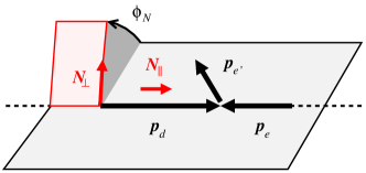
Figure 2: The experimental deuteron polarization in a frame where the deuteron and electron momenta are collinear (beam axis). The vectors $\bm{N}_{\parallel}$ and $\bm{N}_{\perp}$ indicate the directions of parallel and perpendicular polarization. The angle $\phi_{N}$ of $\bm{N}_{\perp}$ is measured relative to the plane defined by the beam axis and the scattered electron momentum.

In pure deuteron spin states polarized parallel to the beam axis, the polarization 4-vector is of the form Eq. (23),

$$s_{d}^{\mu}\;=\;\Lambda_{d}N^{\mu},\hskip 20.00003ptp_{d}N\;=\;0,\hskip 20.00003ptN^{2}\;=\;-1.$$ (80)

The 4-vector $N$ can be expanded covariantly in the electron and deuteron 4-momentum as

$$N^{\mu} = \frac{1}{M_{d}}\left[p_{d}^{\mu}-\frac{M_{d}^{2}}{(p_{e}p_{d})}p_{e}^{\mu}\right].$$ (81)

In the deuteron rest frame its components are

$$N^{\mu}[\textrm{RF}]=\left(0,-\frac{\bm{p}_{e}}{|\bm{p}_{e}|}\right),$$ (82)

and one sees that $\Lambda_{d}=+1\;(-1)$ corresponds to deuteron polarization opposite to the direction (in the direction) of the electron momentum. The effective vector polarizations Eq. (71) are calculated as contractions of Eq. (80), using Eq. (67b) and (72). We obtain

$$S_{L}\; =\;\frac{1+\gamma^{2}y/2}{\sqrt{1+\gamma^{2}}}\;\Lambda_{d},$$ (83a)

$$S_{T}\cos\phi_{S}\; =\;-\frac{\gamma\sqrt{1-y-\gamma^{2}y^{2}/4}}{\sqrt{1+\gamma^{2}}}\;\Lambda_{d},$$ (83b)

$$S_{T}\sin\phi_{S}\; =\;0.$$ (83c)

The polarization 4-tensor in the same pure states is given by the general formula Eq. (26), with the unit vector $N$ of Eq. (81) and the spin projection $\Lambda_{d}$. The effective tensor polarizations, Eq. (77), are calculated as contractions of that 4-tensor. In the case $\Lambda_{d}=\pm 1$ they can be obtained from the vector polarizations Eq. (83) as

$$T_{LL} =\frac{1}{6}\left(3S_{L}^{2}-1\right),$$ (84a)

$$T_{LT}\cos\phi_{T_{L}} =\frac{1}{2}S_{L}S_{T}\cos\phi_{S},$$ (84b)

$$T_{LT}\sin\phi_{T_{L}} =\frac{1}{2}S_{L}S_{T}\sin\phi_{S},$$ (84c)

$$T_{TT}\cos 2\phi_{T_{T}} =\frac{1}{2}S_{T}^{2}(\cos^{2}\phi_{S}-\sin^{2}\phi_{S})$$ (84d)

$$\hskip 10.00002pt[\textrm{$\Lambda_{d}=\pm 1$ only}].$$

The explicit expressions are

$$T_{LL} =\frac{1}{6}\left[\frac{3(1+\gamma^{2}y/2)^{2}}{1+\gamma^{2}}-1\right],$$ (85a)

$$T_{LT}\cos\phi_{T_{L}} =\frac{1}{2}\,\frac{\gamma(1+\gamma^{2}y/2)\sqrt{1-y-\gamma^{2}y^{2}/4}}{1+\gamma^{2}},$$ (85b)

$$T_{LT}\sin\phi_{T_{L}} =0,$$ (85c)

$$T_{TT}\cos 2\phi_{T_{T}} =\frac{1}{2}\;\frac{\gamma^{2}\left(1-y-\gamma^{2}y^{2}/4\right)}{1+\gamma^{2}}$$ (85d)

$$\hskip 10.00002pt[\textrm{$\Lambda_{d}=\pm 1$}].$$ (85e)

In the case $\Lambda_{d}=0$ the effective tensor polarizations are given by $(-2)$ times the expressions in Eq. (85), cf. Eq. (26).

In pure deuteron spin states polarized perpendicular to the beam direction, the deuteron polarization vector is again of the form of Eq. (23) and Eq. (80), but with a different 4-vector $N$, satisfying the conditions

$$p_{e}N\;=\;0,\hskip 20.00003ptp_{d}N\;=\;0,\hskip 20.00003ptN^{2}=-1$$ (86)

(in a frame where $\bm{p}_{e}$ and $\bm{p}_{d}$ are collinear, the first two conditions require that $\bm{p}_{e}\bm{N}=0$). An explicit representation can be found by expanding the 4-vector in the basis Eq. (69) and imposing the conditions Eq. (86),

$$N^{\mu}\; =\;\cos\phi_{N}\;\frac{(e_{T1}p_{e})\,e_{L\ast}^{\mu}-(e_{L\ast}p_{e})\,e_{T1}^{\mu}}{\sqrt{(e_{T1}p_{e})^{2}+(e_{L\ast}p_{e})^{2}}}$$

$$+\;\sin\phi_{N}\,e_{T2}^{\mu}\;,$$ (87)

where the angle $\phi_{N}$ is a free parameter. In the deuteron rest frame the vector components become

$$N^{\mu}[\textrm{RF}]\; =\;(0,\,\bm{N}),\hskip 20.00003pt\bm{p}_{e}\bm{N}\;=\;0,$$ (88a)

$$\bm{N}\; =\;\cos\phi_{N}\,\frac{\bm{p}_{e^{\prime}}-(\bm{p}_{e}\bm{p}_{e^{\prime}})\bm{p}_{e}/|\bm{p}_{e}|^{2}}{\sqrt{|\bm{p}_{e^{\prime}}|^{2}-(\bm{p}_{e}\bm{p}_{e^{\prime}})^{2}/|\bm{p}_{e}|^{2}}}$$

$$+\;\sin\phi_{N}\,\frac{\bm{p}_{e^{\prime}}\times\bm{p}_{e}}{|\bm{p}_{e^{\prime}}\times\bm{p}_{e}|},$$ (88b)

and one identifies $\phi_{N}$ as the angle of the polarization direction relative to the plane spanned by the vectors $\bm{p}_{e}$ and $\bm{p}_{e^{\prime}}$ (electron scattering plane). With the polarization 4-vector given by Eqs. (80) and (87), the effective vector polarizations Eq. (71) for perpendicular polarization are evaluated in the same manner as in the case of parallel polarization, and we obtain

$$S_{L} =\frac{\gamma\sqrt{1-y-\gamma^{2}y^{2}/4}}{\sqrt{1+\gamma^{2}}}\;\cos\phi_{N}\;\Lambda_{d},$$ (89a)

$$S_{T}\cos\phi_{S} =\frac{1+\gamma^{2}y/2}{\sqrt{1+\gamma^{2}}}\;\cos\phi_{N}\;\Lambda_{d},$$ (89b)

$$S_{T}\sin\phi_{S} =\sin\phi_{N}\;\Lambda_{d}.$$ (89c)

The deuteron polarization tensor in the perpendicular polarized states is again given by the general formula Eq. (26), with the unit vector $N$ given by Eq. (87). The effective tensor polarizations for perpendicular polarization are evaluated in the same manner as for parallel polarization. In the case $\Lambda_{d}=\pm 1$ they again can be obtained from the perpendicular vector polarizations Eq. (89) through the relations Eq. (84). The explicit expressions are

$$T_{LL} =\frac{1}{6}\left[\frac{3\gamma^{2}(1-y-\gamma^{2}y^{2}/4)}{1+\gamma^{2}}\cos^{2}\phi_{N}-1\right],$$ (90a)

$$T_{LT}\cos\phi_{T_{L}} =\frac{1}{2}\frac{\gamma(1+\gamma^{2}y/2)\sqrt{1-y-\gamma^{2}y^{2}/4}}{1+\gamma^{2}}$$

$$\times\;\cos^{2}\phi_{N},$$ (90b)

$$T_{LT}\sin\phi_{T_{L}} =\frac{1}{2}\;\frac{\gamma\sqrt{1-y-\gamma^{2}y^{2}/4}}{\sqrt{1+\gamma^{2}}}\;\cos\phi_{N}\sin\phi_{N},$$ (90c)

$$T_{TT}\cos 2\phi_{T_{T}} =\frac{1}{2}\left[\frac{1+\gamma^{2}y+\gamma^{4}y^{2}/4}{1+\gamma^{2}}\cos^{2}\phi_{N}-\sin^{2}\phi_{N}\right]$$ (90d)

$$\hskip 10.00002pt[\textrm{$\Lambda_{d}=\pm 1$}].$$

In the case $\Lambda_{d}=0$ the effective tensor polarizations are given by $(-2)$ times the expressions in Eq. (90).

The effective polarizations depend on the kinematic variables $x_{d},y$ and $Q^{2}$. For a fixed $ed$ collision energy, $y$ is determined by $x_{d}$ and $Q^{2}$, and the polarizations are functions of $x_{d}$ and $Q^{2}$ only. For the following applications it is useful to study their scaling behavior in the DIS limit, $Q^{2}\rightarrow\infty$ with $x_{d}$ fixed. The effective vector polarizations Eqs. (83) and (89) scale as

$$\{S_{L},\,S_{T}\cos\phi_{S}\} ={\mathcal{O}}\{1,\,\gamma\} \parallel$$ ( pol.), (91a)

$$\{S_{L},\,S_{T}\cos\phi_{S},\,S_{T}\sin\phi_{S}\} ={\mathcal{O}}\{\gamma,\,1,\,1\} \perp$$ ( pol.), (91b)

where $\gamma=2x_{d}M_{d}/Q$ is the parameter governing kinematic power corrections, cf. Eq. (42c). Thus $\parallel$ polarization along the beam axis induces mostly $L$ polarization, while $\perp$ polarization induces mostly $T$ polarization, as expected. The scaling behavior of the effective tensor polarizations follows from that of the vector polarizations, cf. Eqs. (85) and (90),

$$\{T_{LL},\,T_{LT}\cos\phi_{T_{L}},\,T_{LT}\sin\phi_{T_{L}},\,T_{TT}\cos 2\phi_{T_{T}}\}$$

$$=\;\left\{\begin{array}[]{ll}{\mathcal{O}}\{1,\,\gamma,\,0,\,\gamma^{2}\}&\text{($\parallel$ pol.)}\\[8.61108pt] {\mathcal{O}}\{1,\,\gamma,\,\gamma,\,1\}&\text{($\perp$ pol.)}\end{array}\right\}.$$ (94)

$T_{LL}$ is of order unity for both $\parallel$ and $\perp$ deuteron polarization. Other than it, the only tensor polarization that is not power-suppressed in the DIS limit is $T_{TT}\cos 2\phi_{T_{T}}$ for $\perp$ deuteron polarization. Note that these statements refer to the kinematic scaling of the effective polarizations, not to the dynamical scaling of the structure functions.

In this section we have derived the effective polarizations for the two idealized situations of pure deuteron spin states polarized parallel or perpendicular to the beam direction (in a frame where the deuteron and electron momenta are collinear). More complex experimental situations can be treated as a superposition of the cases considered here: the cross section is linear in the deuteron density matrix, and more general polarization vectors/tensors can be represented as sums of the ones considered here. This includes the case of colliding-beam experiments with finite crossing angle at an EIC Aschenauer et al. (2014); Abeyratne et al. (2012).

III.7 Spin asymmetries

Experiments typically measure sums and differences of cross sections in different electron and deuteron polarization states and their ratios (spin asymmetries). We now derive the expressions for the spin asymmetries between pure deuteron spin states polarized parallel or perpendicular to the beam axis (see Sec. III.6). We consider the asymmetries formed with all three deuteron spin states ($\Lambda_{d}=\pm 1,0$) and those formed with the two maximum-spin states only ($\Lambda_{d}=\pm 1$) and compare their properties. In the following we write the dependence of the differential cross section Eq. (78) on the electron and deuteron spin projections as

$$d\sigma_{\parallel}(\Lambda_{e},\Lambda_{d}),\hskip 20.00003ptd\sigma_{\perp}(\Lambda_{e},\Lambda_{d}),$$ (95)

where $\parallel$ and $\perp$ distinguish parallel and perpendicular deuteron polarization with respect to the beam axis.

We first consider sums of the cross section over deuteron spin states. The average of the cross section in all three deuteron spin states is

$$\frac{1}{3}\left[d\sigma_{\parallel}(\pm{\textstyle\frac{1}{2}},+1)+d\sigma_{\parallel}(\pm{\textstyle\frac{1}{2}},-1)+d\sigma_{\parallel}(\pm{\textstyle\frac{1}{2}},0)\right]$$

$$= \frac{1}{3}\left[d\sigma_{\perp}(\pm{\textstyle\frac{1}{2}},+1)+d\sigma_{\perp}(\pm{\textstyle\frac{1}{2}},-1)+d\sigma_{\perp}(\pm{\textstyle\frac{1}{2}},0)\right]$$

$$= \;[...]\left(F_{[UU,T]d}\;+\;\epsilon F_{[UU,L]d}\right),$$ (96)

where $[...]$ denotes the differential phase space and flux factors of Eq. (78). The average involves only the unpolarized structure functions. The result is the same when averaging over $\parallel$ and $\perp$ deuteron spin states. It does not depend on the electron spin [as expressed by the notation $\pm\frac{1}{2}$ in Eq. (96)], so that no additional averaging over the electron spin is required in order to isolate the unpolarized structure functions.

The averages of the cross section in the two deuteron spin states with projection $\pm 1$ only are

$$\frac{1}{2}\left[d\sigma_{\parallel}(\pm{\textstyle\frac{1}{2}},+1)+d\sigma_{\parallel}(\pm{\textstyle\frac{1}{2}},-1)\right]$$

$$=\;[...]\left[F_{[UU,T]d}\;+\;\epsilon F_{[UU,L]d}\right.$$

$$+\;D_{\parallel[T_{LL}]}\,\left(F_{[UT_{LL},T]d}+\epsilon F_{[UT_{LL},L]d}\right)$$

$$+\left.D_{\parallel[UT_{LT}]}F_{[UT_{LT}]d}\;+\;D_{\parallel[T_{TT}]}F_{[UT_{TT}]d}\right],$$ (97)

$$\frac{1}{2}\left[d\sigma_{\perp}(\pm{\textstyle\frac{1}{2}},+1)+d\sigma_{\perp}(\pm{\textstyle\frac{1}{2}},-1)\right]$$

$$=\;[...]\left[F_{[UU,T]d}\;+\;\epsilon F_{[UU,L]d}\right.$$

$$+\;D_{\perp[T_{LL}]}\,\left(F_{[UT_{LL},T]d}+\epsilon F_{[UT_{LL},L]d}\right)$$

$$+\;D_{\perp[UT_{LT}]}F_{[UT_{LT}]d}\;+\;D_{\perp[T_{TT}]}F_{[UT_{TT}]d}$$

$$\;\pm\left.D_{\perp[LT_{LT}]}F_{[LT_{LT}]d}\right].$$ (98)

They involve the unpolarized and tensor-polarized structure functions. The functions $D_{(...)}$ (“depolarization factors”) are given by

$$D_{\parallel[T_{LL}]}\;=\;T_{LL}[\Lambda_{d}=\pm 1]$$

$$=\frac{1}{6}\left[\frac{3(1+\gamma^{2}y/2)^{2}}{1+\gamma^{2}}-1\right],$$ (99a)

$$D_{\parallel[UT_{LT}]}\;=\;\sqrt{2\epsilon(1+\epsilon)}\;T_{LT}\cos\phi_{T_{L}}[\Lambda_{d}=\pm 1]$$

$$=\frac{\gamma(1+\gamma^{2}y/2)(1-y-\gamma^{2}y^{2}/4)(1-y/2)}{(1+\gamma^{2})(1-y+y^{2}/2+\gamma^{2}y^{2}/4)},$$ (99b)

$$D_{\parallel[T_{TT}]}\;=\;\epsilon\;T_{TT}\cos 2\phi_{T_{T}}[\Lambda_{d}=\pm 1]$$

$$=\frac{1}{2}\;\frac{\gamma^{2}(1-y-\gamma^{2}y^{2}/4)^{2}}{(1+\gamma^{2})(1-y+y^{2}/2+\gamma^{2}y^{2}/4)};$$ (99c)

$$D_{\perp[T_{LL}]}\;=\;T_{LL}[\Lambda_{d}=\pm 1]$$

$$=\frac{1}{6}\left[\frac{3\gamma^{2}(1-y-\gamma^{2}y^{2}/4)}{1+\gamma^{2}}\cos^{2}\phi_{N}-1\right],$$ (100a)

$$D_{\perp[UT_{LT}]}\;=\;\sqrt{2\epsilon(1+\epsilon)}\;T_{LT}\cos\phi_{T_{L}}[\Lambda_{d}=\pm 1]$$

$$=\frac{\gamma(1+\gamma^{2}y/2)(1-y-\gamma^{2}y^{2}/4)(1-y/2)}{(1+\gamma^{2})(1-y+y^{2}/2+\gamma^{2}y^{2}/4)}\;\cos^{2}\phi_{N},$$ (100b)

$$D_{\perp[LT_{LT}]}\;=\;\sqrt{2\epsilon(1-\epsilon)}\;T_{LT}\sin\phi_{T_{L}}[\Lambda_{d}=\pm 1]$$

$$=\frac{1}{2}\;\frac{\gamma y(1-y-\gamma^{2}y^{2}/4)}{1-y+y^{2}/2+\gamma^{2}y^{2}/4}\;\cos\phi_{N}\sin\phi_{N}.$$ (100c)

$$D_{\perp[T_{TT}]}\;=\;\epsilon\;T_{TT}\cos 2\phi_{T_{T}}[\Lambda_{d}=\pm 1]$$

$$=\;\frac{1}{2}\left(\frac{1+\gamma^{2}y+\gamma^{4}y^{2}/4}{1+\gamma^{2}}\cos^{2}\phi_{N}-\sin^{2}\phi_{N}\right)$$

$$\times\;\frac{1-y-\gamma^{2}y^{2}/4}{1-y+y^{2}/2+\gamma^{2}y^{2}/4},$$ (100d)

In Eq. (99) $T_{LL}$ etc. are the effective tensor polarizations for $\parallel$ polarization with $\Lambda_{d}=\pm 1$ as given in Eq. (85); in Eq. (100) they are the same quantities for $\perp$ polarization as given in Eq. (90). Note that the results are different for $\parallel$ and $\perp$ polarization. In the case of $\parallel$ polarization, Eq. (97), the summation over the two deuteron spin states has canceled all electron-spin dependent terms in Eq. (78), so that the result is independent of the electron spin. It is therefore not necessary to average explicitly over the electron spin. In the case of $\perp$ polarization, Eq. (98), the summation over the two deuteron spin states leaves intact the electron spin-dependent term in Eq. (78),

$$\sim(2\Lambda_{e})T_{LT}\sin\phi_{T_{L}}\;F_{[LT_{LT}]d}.$$ (101)

One must therefore average explicitly over the electron spins if one wants to remove the electron spin dependence.

We now turn to differences of the cross section between deuteron spin states. Here we must take into account that the tagged DIS cross section Eq. (78) contains the term

$$\sim S_{T}\sin\phi_{S}\;F_{[US_{T}]d},$$ (102)

which depends on the deuteron spin but not on the electron spin. In order to isolate the electron spin-dependent structure functions $F_{[LS_{L}]}$ and $F_{[LS_{T}]}$ we form double spin differences with respect to both the deuteron and electron spin, in which the single-spin dependent term Eq. (102) drops out. The double differences of the cross section with respect to the deuteron spin $\pm 1$ ($\parallel$ or $\perp$) and the electron spin are given by

$$\frac{1}{4}\left[d\sigma_{\parallel}(+{\textstyle\frac{1}{2}},+1)-d\sigma_{\parallel}(-{\textstyle\frac{1}{2}},+1)\right.$$

$$\left.-d\sigma_{\parallel}(+{\textstyle\frac{1}{2}},-1)+d\sigma_{\parallel}(-{\textstyle\frac{1}{2}},-1)\right]$$

$$= \;[...]\left(D_{\parallel[S_{L}]}\;F_{[LS_{L}]d}\;+\;D_{\parallel[S_{T}]}\;F_{[LS_{T}]d}\right),$$ (103)

$$\frac{1}{4}\left[d\sigma_{\perp}(+{\textstyle\frac{1}{2}},+1)-d\sigma_{\perp}(-{\textstyle\frac{1}{2}},+1)\right.$$

$$\left.-d\sigma_{\perp}(+{\textstyle\frac{1}{2}},-1)+d\sigma_{\perp}(-{\textstyle\frac{1}{2}},-1)\right]$$

$$= \;[...]\left(D_{\perp[S_{L}]}\;F_{[LS_{L}]d}\;+\;D_{\perp[S_{T}]}\;F_{[LS_{T}]d}\right),$$ (104)

where the depolarization factors are

$$D_{\parallel[S_{L}]} =\sqrt{1-\epsilon^{2}}\;S_{L}[\Lambda_{d}=1]$$

$$=\frac{y(1-y/2)(1+\gamma^{2}y/2)}{1-y+y^{2}/2+\gamma^{2}y^{2}/4},$$ (105a)

$$D_{\parallel[S_{T}]} =\sqrt{2\epsilon(1-\epsilon)}\;S_{T}\cos\phi_{S}[\Lambda_{d}=1]$$

$$=\frac{-\gamma y(1-y-\gamma^{2}y^{2}/4)}{1-y+y^{2}/2+\gamma^{2}y^{2}/4};$$ (105b)

$$D_{\perp[S_{L}]} =\sqrt{1-\epsilon^{2}}\;S_{L}[\Lambda_{d}=1]$$

$$=\frac{\gamma y(1-y/2)\sqrt{1-y-\gamma^{2}y^{2}/4}}{1-y+y^{2}/2+\gamma^{2}y^{2}/4}\cos\phi_{N},$$ (106a)

$$D_{\perp[S_{T}]} =\sqrt{2\epsilon(1-\epsilon)}\;S_{T}\cos\phi_{S}[\Lambda_{d}=1]$$

$$=\frac{y(1+\gamma^{2}y/2)\sqrt{1-y-\gamma^{2}y^{2}/4}}{1-y+y^{2}/2+\gamma^{2}y^{2}/4}\cos\phi_{N}.$$ (106b)

In Eq. (105) $S_{L}$ and $S_{T}\cos\phi_{S}$ are the effective vector polarizations for $\parallel$ polarization with $\Lambda_{d}=1$ as given in Eq. (83); in Eq. (106) they are the same quantities for $\perp$ polarization as given in Eq. (89).

From the spin sums and differences one can form two different ratios (spin asymmetries). The ratios of the spin differences Eqs. (103) and (104) to the three-state average of the cross section Eq. (96) are

$$A_{\parallel(3)d} \equiv \frac{\frac{1}{4}\left[d\sigma_{\parallel}(+{\textstyle\frac{1}{2}},+1)-d\sigma_{\parallel}(-{\textstyle\frac{1}{2}},+1)-d\sigma_{\parallel}(+{\textstyle\frac{1}{2}},-1)+d\sigma_{\parallel}(-{\textstyle\frac{1}{2}},-1)\right]}{\frac{1}{6}\left[d\sigma_{\parallel}(+{\textstyle\frac{1}{2}},+1)+d\sigma_{\parallel}(-{\textstyle\frac{1}{2}},+1)+d\sigma_{\parallel}(+{\textstyle\frac{1}{2}},-1)+d\sigma_{\parallel}(-{\textstyle\frac{1}{2}},-1)+d\sigma_{\parallel}(+{\textstyle\frac{1}{2}},0)+d\sigma_{\parallel}(-{\textstyle\frac{1}{2}},0)\right]}$$ (107)

$$= \frac{D_{\parallel[S_{L}]}\;F_{[LS_{L}]d}\;+\;D_{\parallel[S_{T}]}\;F_{[LS_{T}]d}}{F_{[UU,T]d}\;+\;\epsilon F_{[UU,L]d}},$$

$$A_{\perp(3)d} \equiv \frac{\frac{1}{4}\left[d\sigma_{\perp}(+{\textstyle\frac{1}{2}},+1)-d\sigma_{\perp}(-{\textstyle\frac{1}{2}},+1)-d\sigma_{\perp}(+{\textstyle\frac{1}{2}},-1)+d\sigma_{\perp}(-{\textstyle\frac{1}{2}},-1)\right]}{\frac{1}{6}\left[d\sigma_{\perp}(+{\textstyle\frac{1}{2}},+1)+d\sigma_{\perp}(-{\textstyle\frac{1}{2}},+1)+d\sigma_{\perp}(+{\textstyle\frac{1}{2}},-1)+d\sigma_{\perp}(-{\textstyle\frac{1}{2}},-1)+d\sigma_{\perp}(+{\textstyle\frac{1}{2}},0)+d\sigma_{\perp}(-{\textstyle\frac{1}{2}},0)\right]}$$ (108)

$$= \frac{D_{\perp[S_{L}]}\;F_{[LS_{L}]d}\;+\;D_{\perp[S_{T}]}\;F_{[LS_{T}]d}}{F_{[UU,T]d}\;+\;\epsilon F_{[UU,L]d}}.$$

[Here we have written the denominator as a sum over the electron spin in order to emphasize the similarity with the numerator; because the expression in Eq. (96) is independent of the electron spin this sum is optional and we could just as well use the expression for a fixed electron spin.] The ratios of the spin differences Eqs. (103) and (104) to the two-state averages of the cross section, Eqs. (97) and Eqs. (98), are

$$A_{\parallel(2)d} \equiv\frac{\frac{1}{4}\left[d\sigma_{\parallel}(+{\textstyle\frac{1}{2}},+1)-d\sigma_{\parallel}(-{\textstyle\frac{1}{2}},+1)-d\sigma_{\parallel}(+{\textstyle\frac{1}{2}},-1)+d\sigma_{\parallel}(-{\textstyle\frac{1}{2}},-1)\right]}{\frac{1}{4}\left[d\sigma_{\parallel}(+{\textstyle\frac{1}{2}},+1)+d\sigma_{\parallel}(-{\textstyle\frac{1}{2}},+1)+d\sigma_{\parallel}(+{\textstyle\frac{1}{2}},-1)+d\sigma_{\parallel}(-{\textstyle\frac{1}{2}},-1)\right]}$$

$$=\frac{D_{\parallel[S_{L}]}\;F_{[LS_{L}]d}\;+\;D_{\parallel[S_{T}]}\;F_{[LS_{T}]d}}{F_{[UU,T]d}\;+\;\epsilon F_{[UU,L]d}\;+\;D_{\parallel[T_{LL}]}\,(F_{[UT_{LL},T]d}+\epsilon F_{[UT_{LL},L]d})\;+\;D_{\parallel[UT_{LT}]}\,F_{[UT_{LT}]d}\;+\;D_{\parallel[T_{TT}]}F_{[UT_{TT}]d}}$$ (109)

$$A_{\perp(2)d} \equiv\frac{\frac{1}{4}\left[d\sigma_{\perp}(+{\textstyle\frac{1}{2}},+1)-d\sigma_{\perp}(-{\textstyle\frac{1}{2}},+1)-d\sigma_{\perp}(+{\textstyle\frac{1}{2}},-1)+d\sigma_{\perp}(-{\textstyle\frac{1}{2}},-1)\right]}{\frac{1}{4}\left[d\sigma_{\perp}(+{\textstyle\frac{1}{2}},+1)+d\sigma_{\perp}(-{\textstyle\frac{1}{2}},+1)+d\sigma_{\perp}(+{\textstyle\frac{1}{2}},-1)+d\sigma_{\perp}(-{\textstyle\frac{1}{2}},-1)\right]}$$

$$=\frac{D_{\perp[S_{L}]}\;F_{[LS_{L}]d}\;+\;D_{\perp[S_{T}]}\;F_{[LS_{T}]d}}{F_{[UU,T]d}\;+\;\epsilon F_{[UU,L]d}\;+\;D_{\perp[T_{LL}]}\,(F_{[UT_{LL},T]d}+\epsilon F_{[UT_{LL},L]d})\;+\;D_{\perp[UT_{LT}]}\,F_{[UT_{LT}]d}\;+\;D_{\perp[T_{TT}]}\,F_{[UT_{TT}]d}}.$$ (110)

Now the tensor-polarized structure functions appear in the denominators with the depolarization factors Eqs. (99) and (100). Both the three-state asymmetries, $A_{\parallel(3)d}$ and $A_{\perp(3)d}$, and the two-state asymmetries, $A_{\parallel(2)d}$ and $A_{\perp(2)d}$, can be used for neutron structure extraction from tagged DIS and other spin physics studies and are calculated below.

The scaling behavior of the depolarization factors in the DIS limit can be inferred from that of the effective polarizations, Eqs. (91) and (91), and from the explicit expressions given above,

$$\{D_{\parallel[S_{L}]},D_{\parallel[S_{T}]}\} ={\mathcal{O}}\{1,\gamma\},$$ (111)

$$\{D_{\parallel[T_{LL}]},\,D_{\parallel[UT_{LT}]},\,D_{\parallel[T_{TT}]}\} ={\mathcal{O}}\{1,\gamma,\gamma^{2}\},$$ (112)

$$\{D_{\perp[S_{L}]},D_{\perp[S_{T}]}\} ={\mathcal{O}}\{\gamma,1\},$$ (113)

$$\{D_{\perp[T_{LL}]},D_{\perp[UT_{LT}]},D_{\perp[LT_{LT}]},D_{\perp[T_{TT}]}\} ={\mathcal{O}}\{1,\,\gamma,\gamma,\,1\}.$$ (114)

Up to power corrections ${\mathcal{O}}(\gamma)$, the three-state and two-state asymmetries therefore simplify to

$$A_{\parallel(3)d} =\frac{D_{\parallel[S_{L}]}\;F_{[LS_{L}]d}}{F_{[UU,T]d}\;+\;\epsilon F_{[UU,L]d}},$$ (115)

$$A_{\parallel(2)d} =\frac{D_{\parallel[S_{L}]}\;F_{[LS_{L}]d}}{F_{[UU,T]d}\;+\;\epsilon F_{[UU,L]d}\;+\;D_{\parallel[T_{LL}]}\,(F_{[UT_{LL},T]d}+\epsilon F_{[UT_{LL},L]d})},$$ (116)

$$A_{\perp(3)d} =\frac{D_{\perp[S_{T}]}\;F_{[LS_{T}]d}}{F_{[UU,T]d}\;+\;\epsilon F_{[UU,L]d}},$$ (117)

$$A_{\perp(2)d} =\frac{D_{\perp[S_{T}]}\;F_{[LS_{T}]d}}{F_{[UU,T]d}\;+\;\epsilon F_{[UU,L]d}\;+\;D_{\perp[T_{LL}]}\,(F_{[UT_{LL},T]d}+\epsilon F_{[UT_{LL},L]d})\;+\;D_{\perp[T_{TT}]}\,F_{[UT_{TT}]d}}.$$ (118)

Note that, with our definition of the structure functions, all asymmetries are ${\mathcal{O}}(1)$ in the DIS limit. In the asymmetries for $\parallel$ polarization, the numerators involve the longitudinal spin structure function $F_{[LS_{L}]d}$. The denominator of $A_{\parallel(2)d}$ differs from that of $A_{\parallel(3)d}$ by the tensor-polarized term $F_{[UT_{LL},T]d}+\epsilon F_{[UT_{LL},L]d}$, which has a form similar to the unpolarized term $F_{[UU,T]d}+\epsilon F_{[UU,L]d}$ (this will become apparent in the dynamical calculations below). In the asymmetries for $\perp$ polarization, the numerators involve the transverse spin structure function $F_{[LS_{T}]d}$. The denominator of $A_{\perp(2)d}$ differs from that of $A_{\perp(3)d}$ by two independent tensor-polarized terms and thus has a more complex structure.

For reference we note that in terms of the conventional structure functions the three-state asymmetries Eqs. (107) and (108) are expressed as

$$A_{\parallel(3)d}\; = \;\frac{D_{\parallel 1}g_{1d}\,+\,D_{\parallel 2}g_{2d}}{2(1+\epsilon R_{d})F_{1d}},$$ (119)

$$A_{\perp(3)d}\; = \;\frac{D_{\perp 1}g_{1d}\,+\,D_{\perp 2}g_{2d}}{2(1+\epsilon R_{d})F_{1d}},$$ (120)

where the depolarization factors are now given by

$$D_{\parallel 1} =\;2(D_{\parallel[S_{L}]}-\gamma D_{\parallel[S_{T}]})$$

$$=\;\frac{2(1+\gamma^{2})y(1-y/2-\gamma^{2}y^{2}/4)}{1-y+y^{2}/2+\gamma^{2}y^{2}/4},$$ (121a)

$$D_{\parallel 2} =\;-2\gamma(\gamma D_{\parallel[S_{L}]}+D_{\parallel[S_{T}]})$$

$$=\;\frac{-\gamma^{2}(1+\gamma^{2})y^{2}}{1-y+y^{2}/2+\gamma^{2}y^{2}/4},$$ (121b)

$$D_{\perp 1}\; =\;2(D_{\perp[S_{L}]}-\gamma D_{\perp[S_{T}]})$$

$$=\;\displaystyle\frac{-\gamma(1+\gamma^{2})y^{2}\sqrt{1-y-\gamma^{2}y^{2}/4}}{1-y+y^{2}/2+\gamma^{2}y^{2}/4}\cos\phi_{N},$$ (122a)

$$D_{\perp 2}\; =\;-2\gamma(\gamma D_{\perp[S_{L}]}+D_{\perp[S_{T}]})$$

$$=\;\displaystyle\frac{-2\gamma(1+\gamma^{2})y\sqrt{1-y-\gamma^{2}y^{2}/4}}{1-y+y^{2}/2+\gamma^{2}y^{2}/4}\cos\phi_{N},$$ (122b)

and scale as

$$\{D_{\parallel 1},D_{\parallel 2}\} ={\mathcal{O}}\{1,\gamma^{2}\},$$ (123)

$$\{D_{\perp 1},D_{\perp 2}\} ={\mathcal{O}}\{\gamma,\gamma\}.$$ (124)

In $A_{\parallel(3)d}$ the structure function $g_{1}$ appears in the scaling limit, while $g_{2}$ appears as a power correction $\sim 1/Q^{2}$. In $A_{\perp(3)d}$ the structure functions $g_{1}$ and $g_{2}$ appear at the same level, but the entire asymmetry is power-suppressed $\sim 1/Q$

III.8 Collinear frames

In the theoretical description of tagged DIS we consider the process Eq. (30) in a frame where the deuteron momentum $\bm{p}_{d}$ and the momentum transfer $\bm{q}$ are collinear and define the $z$–axis of the coordinate system (see Fig. 3). This condition does not specify a unique frame, but rather a class of frames that are related by boosts along the $z$–axis (“collinear frames”). We describe the 4-vectors in this frame by their LF components

$$v^{\pm}\;\;\equiv\;\;v^{0}\pm v^{z},\hskip 20.00003pt\bm{v}_{T}\;\;\equiv\;\;(v^{x},v^{y}),$$ (125)

and use the notation

$$v\;\;=\;\;[v^{+},v^{-},\bm{v}_{T}].$$ (126)

The LF components of the 4-momenta $p_{d}$ and $q$ in the collinear frame are

$$p_{d}\; =\;\left[p_{d}^{+},\;\frac{M_{d}^{2}}{p_{d}^{+}},\;\bm{0}_{T}\right],$$ (127a)

$$q\; =\;\left[-\xi_{d}p_{d}^{+},\;\frac{Q^{2}}{\xi_{d}p_{d}^{+}},\;\bm{0}_{T}\right],$$ (127b)

where the parameter $\xi_{d}$ is related to the scaling variable $x_{d}$

$$\xi_{d}\;\;=\;\;\frac{2x_{d}}{1+\sqrt{1+\gamma^{2}}}\;\;=\;\;x_{d}\;+\;{\mathcal{O}}(\gamma^{2}).$$ (128)

Note that in our convention the 3-vector $\bm{q}$ points in the negative $z$-direction, $q^{z}=(q^{+}-q^{-})/2<0$.

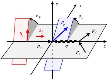
Figure 3: Tagged deuteron DIS in the collinear frame, Eq. (127). The deuteron 3-momentum $\bm{p}_{d}$ and the momentum transfer $\bm{q}$ are collinear and define the $z$-axis ($\bm{q}$ points in the negative $z$-direction). The initial and final electron momenta, $\bm{p}_{e}$ and $\bm{p}_{e^{\prime}}$, define the $xz$ plane (both have positive $x$ components). The deuteron vector polarization is described by the longitudinal ($z$-) spin $S_{L}$ and the transverse ($xy$-) spin vector $\bm{S}_{T}$ (the azimuthal angle $\phi_{S}$ is measured relative to the positive $x$ axis). The tagged proton momentum $\bm{p}_{p}$ has both longitudinal and transverse components (azimuthal angle $\phi_{p}$).

The collinear frames are a class of frames related by boosts along the $z$-axis (longitudinal boosts). The boosts are performed by changing the LF components of the 4-vectors as

$$[v^{+},v^{-},\bm{v}_{T}]\;\rightarrow\;[e^{\eta}v^{+},e^{-\eta}v^{-},\bm{v}_{T}],$$ (129)

where $\eta$ is the rapidity. If the $+$ and $-$ components are expressed as multiples of $p_{d}^{+}$ and $1/p_{d}^{+}$, the boosts can be effected by simply changing the value of $p_{d}^{+}$ from the one in the “old” frame to the one in the “new” frame. In this sense $p_{d}^{+}$ serves as a parameter that identifies a particular representative of the class. In particular, the class of collinear frames includes the deuteron rest frame, in which

$$p_{d}^{+}=M_{d}.$$ (130)

In this way one can construct a boost-invariant theoretical description that can easily be matched with the deuteron rest frame. The deuteron polarization 4-vector in any collinear frame is given by

$$s_{d} = \left[\frac{p_{d}^{+}}{M_{d}}S_{d}^{z},-\frac{M_{d}}{p_{d}^{+}}S_{d}^{z},\bm{S}_{dT}\right],$$ (131)

where $S_{d}^{z}$ and $\bm{S}_{dT}\equiv(S_{d}^{x},S_{d}^{y})$ are the components of the polarization 3-vector in the rest frame, cf. Eq. (19a),

$$\bm{S}_{d}\; =\;(\bm{S}_{dT},S_{d}^{z}),$$ (132a)

$$|\bm{S}_{d}|^{2}\; =\;(S_{d}^{z})^{2}+|\bm{S}_{dT}|^{2}\;\leq\;1.$$ (132b)

In the collinear frames the longitudinal unit 4-vectors Eq. (60) have only $+$ and $-$ components,

$$e_{d}\; =\;\left[\frac{p_{d}^{+}}{M_{d}},\frac{M_{d}}{p_{d}^{+}},\bm{0}_{T}\right],$$ (133a)

$$e_{L\ast}\; =\;\left[-\frac{p_{d}^{+}}{M_{d}},\frac{M_{d}}{p_{d}^{+}},\bm{0}_{T}\right].$$ (133b)

The transverse unit 4-vectors have only transverse components, which are chosen as the $x$ and $y$ directions,

$$e_{T1}\;=\;\left[0,0,\bm{e}_{x}\right],\hskip 20.00003pte_{T2}\;=\;\left[0,0,\bm{e}_{y}\right],$$ (134)

such that the electron scattering plane is the $xz$ plane, and the electron has a transverse momentum along the positive $x$-axis. It is straightforward to compute invariants from these 4-vectors and express them in terms of deuteron rest-frame variables. Specifically, one sees that the invariant effective vector polarization parameters, defined in Eq. (71), coincide with the longitudinal and transverse component of the 3-dimensional deuteron polarization vector in the rest frame

$$S_{L}\; \equiv\;S_{d}^{z},$$ (135a)

$$(S_{T}\cos\phi_{S},\,S_{T}\sin\phi_{S})\; \equiv\;(S_{d}^{x},S_{d}^{y})\;=\;\bm{S}_{dT}.$$ (135b)

The angle $\phi_{S}$ can be regarded as the angle of the transverse component of the deuteron spin in the rest frame (or any collinear frame) relative to electron scattering plane, measured from positive $x$-axis (see Fig. 3).

In a similar way one can infer the form of the deuteron polarization 4-tensor in any collinear frame. For the LF components of a 4-tensor $w^{\mu\nu}$ we use the notation [cf. Eq. (129)]

$$w\;=\;\left[\begin{array}[]{lll}w^{++}&w^{+-}&w^{+j}\\[8.61108pt] w^{-+}&w^{--}&w^{-j}\\[8.61108pt] w^{i+}&w^{i-}&w^{ij}\end{array}\right]\hskip 20.00003pt(i,j=x,y).$$ (136)

The LF components of the deuteron polarization 4-tensor in any collinear frame are then given by

$$t_{d}\; = \;\left[\begin{array}[]{rrr}\displaystyle\frac{(p_{d}^{+})^{2}}{M_{d}^{2}}T_{d}^{zz}&-T_{d}^{zz}&\displaystyle\frac{p_{d}^{+}}{M_{d}}T_{d}^{zj}\\[8.61108pt] -T_{d}^{zz}&\displaystyle\frac{M_{d}^{2}}{(p_{d}^{+})^{2}}T_{d}^{zz}&\displaystyle-\frac{M_{d}}{p_{d}^{+}}T_{d}^{zj}\\[8.61108pt] \displaystyle\frac{p_{d}^{+}}{M_{d}}T_{d}^{zi}&\displaystyle-\frac{M_{d}}{p_{d}^{+}}T_{d}^{zi}&T_{d}^{ij}\end{array}\right],$$ (140)

where $T_{d}^{zz},T_{d}^{zi}$ and $T_{d}^{ij}$ ($i,j=x,y$) are the components of is the deuteron polarization 3-tensor in the rest frame,

$$T_{d}\;=\;\left(\begin{array}[]{rr}T_{d}^{ij}&T_{d}^{iz}\\[8.61108pt] T_{d}^{zj}&T_{d}^{zz}\end{array}\right)\hskip 20.00003pt(i,j=x,y).$$ (141)

Eq. (140) for the polarization 4-tensor is a straightforward generalization of Eq. (131) for the polarization 4-vector.

In experimental or theoretical applications one needs to infer the LF components of a 4-vector in the collinear frame from those given in another frame. This can easily be accomplished using the 4-vector basis Eq. (69). From the timelike and spacelike longitudinal vectors, $e_{d}$ and $e_{L\ast}$, we construct the light-like vectors $e_{d}\pm e_{L\ast}$,

$$(e_{d}\pm e_{L\ast})^{2}=0,\hskip 20.00003pt(e_{d}+e_{L\ast})(e_{d}-e_{L\ast})=2.$$ (142)

Their components in the collinear frame are [cf. Eq. (133)]

$$e_{d}+e_{L\ast}\; =\;\left[0,\frac{2M_{d}}{p_{d}^{+}},\bm{0}_{T}\right],$$ (143a)

$$e_{d}-e_{L\ast}\; =\;\left[\frac{2p_{d}^{+}}{M_{d}},0,\bm{0}_{T}\right].$$ (143b)

The scalar products of the vectors with an arbitrary vector $v$ are

$$(e_{d}+e_{L\ast})\,v\; =\;\frac{M_{d}}{p_{d}^{+}}v^{+},$$ (144a)

$$(e_{d}-e_{L\ast})\,v\; =\;\frac{p_{d}^{+}}{M_{d}}v^{-}.$$ (144b)

They project out the $+$ and $-$ LF components of the vector. The transverse components are projected out as

$$v^{x}=-(e_{T1}v),\hskip 20.00003ptv^{y}=-(e_{T2}v).$$ (145)

The expressions in Eqs. (144) and (145) are invariant and can be used to compute the LF components starting from an arbitrary representation of the vector $v$ and the basis vectors (e.g., in a frame associated with the experimental setup). Conversely, the components of $v$ in any frame can be obtained from the LF components in the collinear frame by expanding $v$ in the basis vectors,

$$v^{\mu}\; =\;\frac{M_{d}}{2p_{d}^{+}}v^{+}(e_{d}+e_{L\ast})^{\mu}+\frac{p_{d}^{+}}{2M_{d}}v^{-}(e_{d}-e_{L\ast})^{\mu}$$

$$+\;v^{x}e_{T1}^{\mu}\;+\;v^{y}e_{T2}^{\mu},$$ (146)

and evaluating the expression with the basis vector components in the desired frame.

III.9 Spectator momentum variables

The invariant structure functions in the tagged DIS cross section Eq. (78) depend on kinematic variables specifying the final-state proton momentum, cf. Eq. (47). Several sets of variables are used in experimental analysis and theoretical studies (proton 3-momentum in deuteron rest frame, LF components in collinear frame, invariant momentum transfer); their relation and kinematic limits are summarized in Ref. Strikman and Weiss (2018). In the following calculations the proton momentum is specified by its LF components in the collinear frames,

$$\alpha_{p}\;\equiv\;\frac{2p_{p}^{+}}{p_{d}^{+}},\hskip 20.00003pt\bm{p}_{pT}.$$ (147)

The fraction $\alpha_{p}$ is boost-invariant (same in all collinear frames) and can be expressed in terms of invariants that can be evaluated in any frame, cf. Eq. (144),

$$\alpha_{p}\;=\;\frac{2(e_{d}+e_{L\ast})p_{p}}{(e_{d}+e_{L\ast})p_{d}};$$ (148)

the same applies to $\bm{p}_{pT}$, cf. Eq. (145). In the deuteron rest frame, $\alpha_{p}$ is given by

$$\alpha_{p}\;\;=\;\;\frac{2(E_{p}+p_{p}^{z})}{M_{d}}\;=\;1\;+\;\frac{p_{p}^{z}}{m}\;+\;{\mathcal{O}}\left(\frac{|\bm{p}_{p}|^{2}}{m^{2}},\frac{\epsilon_{d}}{m}\right),$$ (149)

where $m$ is the nucleon mass and $\epsilon_{d}$ the deuteron binding energy; typical values of $\alpha_{p}$ are therefore of the order

$$|\alpha_{p}-1|\;\;\sim\;\;\frac{|\bm{p}_{p}|}{m}\;\;\lesssim\;\;0.1.$$ (150)

The range of $\alpha_{p}$ is kinematically limited by the conservation of 4-momentum in the tagged DIS process, which implies the conservation of LF plus momentum, Eq. (127),

$$\alpha_{p}/2\;<\;1-\xi_{d}.$$ (151)

The invariant phase space element in the proton momentum is expressed in terms of $\alpha_{p}$ and $\bm{p}_{pT}$ as

$$d\Gamma_{p}\;\equiv\;[2(2\pi)^{3}]^{-1}\;\frac{d^{3}p_{p}}{E_{p}}\;\;=\;\;[2(2\pi)^{3}]^{-1}\;\frac{d\alpha_{p}}{\alpha_{p}}\;d^{2}p_{pT}.$$ (152)

The structure functions in Eq. (78) depend on $\alpha_{p}$ and the modulus of the transverse momentum, $|\bm{p}_{pT}|$. The dependence on the azimuthal angle of the transverse momentum with respect to the $z$ axis, $\phi_{p}$ (see Fig. 3), is realized explicitly in the decomposition of the cross section, which follows from the decomposition of the hadronic tensor; Eq. (78) shows only the terms that are independent of $\phi_{p}$ and survive integration over that variable.

IV Deuteron light-front structure

IV.1 Light-front nuclear structure

We now describe the elements of LF nuclear structure used in the theoretical calculation of the tagged DIS cross section. The basic method was developed in Refs. Frankfurt and Strikman (1981, 1988) and is summarized in Ref. Strikman and Weiss (2018). In this section we present the formalism for the treatment of polarized deuteron structure in the covariant approach of Refs. Kondratyuk and Strikman (1984); Frankfurt and Strikman (1983) and its connection to nonrelativistic deuteron spin structure. The evaluation of nucleonic operators and the calculation of the tagged DIS cross section are discussed in Secs. V and VI.

High-energy processes such as DIS probe the nucleus with energy transfers much larger than the hadronic mass scale and result in hadron production over wide rapidity intervals. One would like to construct a theoretical description that starts from the nucleus as a system of protons and neutrons and produces the DIS final state by scattering on the nucleons, with eventual corrections due to nuclear binding effects. That such an approximation can be obtained is not obvious, as the nuclear initial states relevant for the process might a priori involve states with energies of the order of the excitation energy, which in a relativistic context can no longer be described in terms of nucleonic degrees of freedom. The notion of energy, and therefore the relevant states, depend on the relativistic quantization scheme adopted for the description of the process. LF quantization, which describes the evolution of the process in LF time $x^{+}=t+z$ (with the $z$-direction along the reaction axis), is unique in that the energies of the intermediate states do not grow with the collision energy but remain finite in the high-energy limit. It therefore permits a composite description of the nuclear initial state in terms of nucleon degrees of freedom, which is then matched with the high-energy scattering process on the nucleons, with finite effects due to nuclear binding.

In LF quantization the spin degrees of freedom of particles and composite systems are described by light-front helicity states (see Fig. 4). They are prepared by starting from the spin states in the rest frame, $p^{+}=m$ and $\bm{p}_{T}=0$, quantized along the $z$-direction, performing first a longitudinal boost to the desired plus momentum $p^{+}\neq m$, and then a transverse boost to the desired transverse momentum $\bm{p}_{T}\neq 0$. The states thus defined are invariant under longitudinal boosts and transform kinematically under transverse boosts. They differ from the so-called canonical spin states, which are prepared by performing a standard boost along the particle’s 3-momentum direction as in equal-time quantization, because boosts along different directions do not commute. The difference between the two states is a spin rotation, the so-called Melosh rotation. The explicit form of the nucleon bispinors for LF helicity states and canonical spin states, and the Melosh rotation connecting them, is given in Appendix A. In the following we use a representation of the deuteron LF wave function in which the LF helicity character of the nucleon spin states is encoded in the explicit form of the bispinors and thus no explicit Melosh rotations appear; the rotations are needed only in proving the equivalence of this representation to the 3-dimensional canonical spin structure in the CM frame in Sec. IV.3 and Appendix B.

Figure 4: LF helicity and canonical spin states. The diagram shows the sequence of boosts leading from the rest-frame to the particle state with LF momentum $p^{+}$ and $\bm{p}_{T}$.

IV.2 Light-front wave function in 4-dimensional form

The LF quantization is performed in the collinear frames, Sec. III.8, where the deuteron has LF plus momentum $p_{d}^{+}$ (arbitrary) and transverse momentum $\bm{p}_{dT}=0$; the deuteron 4-momentum components are [cf. Eq. (127)]

$$p_{d}\; = \;\left[p_{d}^{+},\frac{M_{d}^{2}}{p_{d}^{+}},\bm{0}_{T}\right]$$ (153)

The deuteron spin is described by the LF helicity, $\lambda_{d}$, which coincides with the rest-frame spin projection because the states have zero transverse momentum. The expansion of the deuteron state in $pn$ states is described by LF wave function (see Fig. 5)

$$\Psi_{d}(\alpha_{p},\bm{p}_{pT};\lambda_{p},\lambda_{n}|\lambda_{d});$$ (154)

the definition of the matrix element and normalization of the states are given in Ref. Strikman and Weiss (2018). The wave function is normalized such that

$$\sum_{\lambda_{p},\lambda_{n}}\int\frac{d\alpha_{p}\;d^{2}p_{pT}}{\alpha_{p}(2-\alpha_{p})}\;\Psi_{d}^{\ast}(\alpha_{p},\bm{p}_{pT};\lambda_{p},\lambda_{n}|{\lambda^{\prime}}_{\!\!d})$$

$$\times\Psi_{d}(\alpha_{p},\bm{p}_{pT};\lambda_{p},\lambda_{n}|\lambda_{d})\;\;=\;\;\delta({\lambda^{\prime}}_{\!\!d},\lambda_{d}).$$ (155)

It is a function of the proton LF momentum fraction $\alpha_{p}$ and transverse momentum $\bm{p}_{pT}$; the corresponding values for the neutron are

$$\alpha_{n}\;=\;2-\alpha_{p},\hskip 20.00003pt\bm{p}_{nT}\;=\;-\bm{p}_{pT}.$$ (156)

The wave function is symmetric under the interchange of proton and neutron variables (momentum and spin) and satisfies the relation

$$\;\Psi_{d}(\alpha_{p},\bm{p}_{pT};\lambda_{p},\lambda_{n}|\lambda_{d})$$

$$= \;\Psi_{d}(2-\alpha_{p},-\bm{p}_{pT};\lambda_{n},\lambda_{p}|\lambda_{d}).$$ (157)

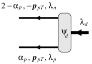
Figure 5: The deuteron LF wave function, Eq. (154), describing the expansion of the deuteron state in $pn$ states.

The spin structure of the deuteron LF wave function can be established on general grounds. It describes the coupling of the proton and neutron LF helicities, and the LF orbital angular momentum, to the overall LF helicity of the deuteron. In the following we use a representation in which this coupling is expressed in 4-dimensional form, through invariants constructed out of the nucleon LF bispinors and a deuteron polarization 4-vector Kondratyuk and Strikman (1984). The LF wave function is written in the form

$$\Psi_{d}(\alpha_{p},\bm{p}_{pT};\lambda_{p},\lambda_{n}|\lambda_{d})$$

$$=\;\bar{u}_{\rm LF}(p_{n},\lambda_{n})\,\Gamma_{\alpha}(p_{p},p_{n})\,v_{\rm LF}(p_{p},\lambda_{p})\;\epsilon_{pn}^{\alpha}(p_{pn},\lambda_{d}).$$ (158)

Here $p_{p}$ and $p_{n}$ are the 4-momenta of the proton and neutron, whose LF components are

$$p_{p}\; =\;\left[\frac{\alpha_{p}p_{d}^{+}}{2},\;\frac{2(|\bm{p}_{pT}^{2}|+m^{2})}{\alpha_{p}p_{d}^{+}},\;\bm{p}_{pT}\right],$$ (159a)

$$p_{n}\; =\;\left[\frac{(2-\alpha_{p})p_{d}^{+}}{2},\;\frac{2(|\bm{p}_{pT}^{2}|+m^{2})}{(2-\alpha_{p})p_{d}^{+}},\;-\bm{p}_{pT}\right],$$ (159b)

$$p_{p}^{2}\; =\;p_{n}^{2}\;=\;m^{2}.$$ (159c)

The LF plus and transverse components are determined by the variables $\alpha_{p}$ and $\bm{p}_{pT}$; the minus components are fixed by the mass-shell conditions Eq. (159c). Furthermore,

$$u_{\rm LF}(p_{n},\lambda_{n}),\hskip 10.00002ptv_{\rm LF}(p_{p},\lambda_{p}),$$ (160a)

$$(p_{n}\gamma-m)u_{\rm LF}=0,\hskip 10.00002pt(p_{p}\gamma+m)v_{\rm LF}=0,$$ (160b)

are the LF bispinor wave functions of the nucleon states with 4-momenta $p_{p}$ and $p_{n}$ and LF helicities $\lambda_{p}$ and $\lambda_{n}$, whose explicit form is given in Appendix A. In Eq. (158), $p_{pn}$ is the total 4-momentum of the $pn$ pair,

$$p_{pn}\; \equiv\;p_{p}+p_{n}\;=\;\displaystyle\left[p_{d}^{+},\;\frac{M_{pn}^{2}}{p_{d}^{+}},\;\bm{0}_{T}\right],$$ (161a)

$$p_{pn}^{2} =\;M^{2}_{pn}\;\equiv\;\frac{4(|\bm{p}_{pT}^{2}|+m^{2})}{\alpha_{p}(2-\alpha_{p})}.$$ (161b)

$M_{pn}$ is known as the invariant mass of the $pn$ pair. Note that the plus and transverse 4-momentum components (LF momenta) of the $pn$ pair are the same as those of the external deuteron state, but the minus component (LF energy) is different,

$$p_{pn}^{+}\; =\;p_{d}^{+},\hskip 20.00003pt\bm{P}_{pn,T}\;=\;\bm{p}_{dT}\;(=\;0),$$ (162a)

$$p_{pn}^{-}\; \neq\;p_{d}^{-},$$ (162b)

and the invariant mass of the $pn$ pair is different from the deuteron mass

$$M_{pn}^{2}\; \neq\;M_{d}^{2}.$$ (163)

These relations reflect the choice of momentum and energy variables specific to LF quantization. Finally, in Eq. (158), $\epsilon_{pn}$ is the 4-vector spin wave function of the $pn$ system with 4-momentum $p_{pn}$ and mass $M_{pn}$,

$$\epsilon_{pn}(p_{pn},\lambda_{d})\;=\;\left[\frac{p_{d}^{+}}{M_{pn}}\epsilon_{d}^{z},-\frac{M_{pn}}{p_{d}^{+}}\epsilon_{d}^{z},\bm{\epsilon}_{dT}\right],$$ (164a)

$$\epsilon_{pn}p_{pn}\;=\;0,\hskip 20.00003pt\epsilon_{pn}^{2}\;=\;-(\epsilon_{d}^{z})^{2}-\bm{\epsilon}_{dT}^{2}\;=\;-1,$$ (164b)

in which $\epsilon_{d}^{z}$ and $\bm{\epsilon}_{dT}\equiv(\epsilon_{d}^{x},\epsilon_{d}^{y})$ are the components of the deuteron 3-vector spin wave function in the deuteron rest frame,

$$\bm{\epsilon}_{d}\;\equiv\;\bm{\epsilon}_{d}(\lambda_{d})\;=\;(\bm{\epsilon}_{dT},\epsilon_{d}^{z}),\hskip 20.00003pt\bm{\epsilon}_{d}^{2}\;=\;1.$$ (165)

Note that the $pn$ 4-vector Eq. (164) is different from the deuteron 4-vector,

$$\epsilon_{d}(p_{d},\lambda_{d}) =\left[\frac{p_{d}^{+}}{M_{d}}\epsilon_{d}^{z},-\frac{M_{d}}{p_{d}^{+}}\epsilon_{d}^{z},\bm{\epsilon}_{dT}\right],$$ (166a)

$$\epsilon_{d}p_{d}\; =0,\hskip 20.00003pt\epsilon_{d}^{2}\;=\;-(\epsilon_{d}^{z})^{2}-\bm{\epsilon}_{dT}^{2}\;=-1.$$ (166b)

The particular form of Eq. (164) is necessary to ensure the equivalence of Eq. (158) with the 3-dimensional spin structure of the $pn$ pair in the CM frame, as explained in Sec. IV.3 and Appendix B.

The function $\Gamma_{\alpha}$ in Eq. (158), a matrix in bispinor space and a 4-vector, connects the nucleon bispinors and the deuteron 4-vector to an invariant form. It may be regarded as a function of the 4-momenta $p_{p}$ and $p_{n}$, and its form is constrained by standard 4-dimensional relativistic covariance. Taking into account the equations for the nucleon spinors, Eq. (160), it can be decomposed in independent covariant structures as

$$\Gamma^{\alpha}\;\equiv\;\Gamma^{\alpha}(p_{p},p_{n})\; = \;\gamma^{\alpha}G_{1}\;+\;\Delta^{\alpha}G_{2},$$ (167)

where $\Delta$ is the difference of the nucleon 4-momenta,

$$\Delta\equiv p_{p}-p_{n},\hskip 10.00002pt\Delta p_{pn}=0,\hskip 10.00002pt\Delta^{2}=-M_{pn}^{2}+4m^{2},$$ (168)

and $G_{1,2}$ are scalar functions of the invariant mass of the $pn$ pair,

$$G_{1,2} \equiv G_{1,2}(M_{pn}).$$ (169)

The functions $G_{1,2}$ contain the dynamical information about deuteron structure in LF quantization. They can be matched with the 3-dimensional radial wave functions in equal-time quantization, and their explicit form is given in Sec. IV.3.

Together, Eqs. (158) and (167) provide a representation of the LF spin structure of the deuteron in 4-dimensional form. Its advantages are: (a) The representation of Eqs. (158) and (167) avoids the use of explicit Melosh rotations, which appear in the standard construction of the LF wave function starting from a 3-dimensional wave function with canonical spinors. The rotations are contained in the explicit form of the LF bispinors. (b) The representation of Eqs. (158) and (167) permits efficient evaluation of the sums over nucleon spin degrees of freedom in observables, given by overlap integrals of the LF wave functions. Sums over the nucleon LF helicities can be converted to traces over spin density matrices in bispinor representation, which can be evaluated using standard techniques. (c) Overall, the representation enables a 4-dimensional treatment of spin structure within the essentially 3-dimensional approach of LF quantization.

IV.3 Center-of-mass frame variables

In the LF wave function Eq. (158) the $pn$ configuration is specified by the LF momentum variables $\alpha_{p}$ and $\bm{p}_{pT}$. An alternative representation of the LF wave function is obtained by using as variables the proton 3-momentum in the CM frame of the $pn$ pair. This representation offers a simple way of realizing rotational invariance in LF quantization, permits matching of the invariant functions Eq. (169) with the equal-time wave functions, and enables the construction of a nonrelativistic approximation to the LF wave functions. In the following calculations we deal with the LF components and the ordinary components of 4-vectors at the same time and use the notation [cf. Eq. (126)]

$$[v^{+},v^{-},\bm{v}_{T}],\hskip 20.00003pt(v^{0},\bm{v}),$$ (170)

to distinguish both sets of components in a given frame.

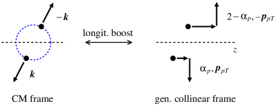
Figure 6: The CM frame variables for the deuteron LF wave function. In a general collinear frame the wave function depends on the longitudinal and transverse momenta, $\alpha_{p}$ and $\bm{p}_{pT}$ (right). By a longitudinal boost any such frame is connected with the CM frame of the $pn$ pair, in which the wave function depends on the 3-momentum $\bm{k}$ and exhibits rotational symmetry (left).

The CM frame of a given $pn$ configuration is defined as the frame in which the proton and neutron have opposite 3-momenta in the sense of ordinary vector components. This frame is a member of the class of collinear frames and can be reached from any other collinear frame by a longitudinal boost (see Fig. 6). To show this, we use the fact that a collinear frame in the class is specified by the value of $p_{d}^{+}$ in that frame (see Sec. III.8). The CM frame of the $pn$ configuration is the special collinear frame with

$$p_{d}^{+}[\textrm{CM}]\;=\;M_{pn}.$$ (171)

In this frame the total 4-momentum of the $pn$ configuration, Eq. (161a), has LF components

$$p_{pn}[\textrm{CM}]\;=\;[M_{pn},M_{pn},\bm{0}_{T}],$$ (172)

and therefore ordinary components

$$p_{pn}[\textrm{CM}]\;=\;(M_{pn},\bm{0}).$$ (173)

The individual proton and neutron 4-momenta have LF components

$$p_{p}[\textrm{CM}] =\left[\frac{\alpha_{p}M_{pn}}{2},\frac{(2-\alpha_{p})M_{pn}}{2},\bm{p}_{pT}\right],$$ (174a)

$$p_{n}[\textrm{CM}] =\left[\frac{(2-\alpha_{p})M_{pn}}{2},\frac{\alpha_{p}M_{pn}}{2},-\bm{p}_{pT}\right],$$ (174b)

such that the ordinary components satisfy (we suppress the label [CM])

$$p_{n}^{0} ={\textstyle\frac{1}{2}}(p_{n}^{+}+p_{n}^{-})\;=\;\phantom{-}{\textstyle\frac{1}{2}}(p_{p}^{+}+p_{p}^{-})\;=\;\phantom{-}p_{p}^{0},$$ (175a)

$$p_{n}^{z} ={\textstyle\frac{1}{2}}(p_{n}^{+}-p_{n}^{-})\;=\;-{\textstyle\frac{1}{2}}(p_{p}^{+}-p_{p}^{-})\;=\;-p_{p}^{z},$$ (175b)

$$\bm{p}_{nT} =-\bm{p}_{pT},$$ (175c)

i.e., they have the same energy and opposite 3-momenta. In this frame the proton and neutron 4-momenta can therefore be expressed in terms of the common 3-momentum vector as

$$p_{p}[\textrm{CM}]\; =\;(E,\bm{k}),$$ (176a)

$$p_{n}[\textrm{CM}]\; =\;(E,-\bm{k}),$$ (176b)

$$E\;\equiv\;E(\bm{k})\; \equiv\;\sqrt{|\bm{k}|^{2}+m^{2}}$$ (176c)

The relation of the CM momentum $\bm{k}$ to the LF variables $\alpha_{p}$ and $\bm{p}_{pT}$ is

$$k^{z}\; =\;\frac{M_{pn}}{2}(\alpha_{p}-1),\hskip 20.00003pt\bm{k}_{T}\;=\;\bm{p}_{pT},$$ (177a)

$$\alpha_{p}\; =\;1+\frac{k^{z}}{E},\hskip 20.00003ptM_{pn}\;=\;2E.$$ (177b)

The CM momentum can therefore serve as a kinematic variable alternative to the LF variables,

$$\bm{k}\;\leftrightarrow\;\{\alpha_{p},\bm{p}_{pT}\}.$$ (178)

The relation between the integration measures is

$$\int\frac{d\alpha_{p}\;d^{2}p_{pT}}{\alpha_{p}(2-\alpha_{p})}\; = \;\int\frac{d^{3}k}{E(k)}.$$ (179)

In the CM frame the polarization vector of the $pn$ system, Eq. (164), has 4-vector components (LF and ordinary)

$$\epsilon_{pn}[\textrm{CM}]\; = \;[\epsilon_{d}^{z},-\epsilon_{d}^{z},\bm{\epsilon}_{dT}]\;=\;(0,\bm{\epsilon}_{d}).$$ (180)

This is the same form that the deuteron polarization vector has in the deuteron rest frame, cf. Eq. (166) with $p_{d}^{+}=M_{d}$. The CM frame thus permits a particularly simple representation of the deuteron spin structure. We use this representation extensively in the calculations in Secs. V and VI.

In the CM frame the $pn$ LF wave function can be can be formulated as a 3-dimensional relativistic wave function in the 3-momentum variable $\bm{k}$. It is constructed using angular momentum wave functions (S and D waves), canonical nucleon spinors, and the Melosh rotations mediating the transition from canonical spin to LF helicity (see Appendix B). The dynamical information is contained in the radial wave functions of the S- and D-waves,

$$f_{0}(k),\;f_{2}(k)\hskip 20.00003pt[k\equiv|\bm{k}|],$$ (181)

which are normalized such that

$$4\pi\int\frac{dk\,k^{2}}{E(k)}\;[f_{0}^{2}(k)+f_{2}^{2}(k)]\;\;=\;\;1.$$ (182)

Using the fact that the CM frame is a special collinear frame, one can then establish the correspondence between the general LF wave function Eq. (158) and the 3-dimensional wave function in the CM frame. The proof involves expressing the LF bispinors in Eq. (158) in terms of canonical bispinors in the CM frame, reducing the bilinear form in the canonical bispinors to two-component spinors, and comparing with the 3-dimensional wave function (see Appendix B). As a result, one obtains the relation between the invariant functions $G_{1,2}(M_{pn}^{2})$, Eq. (169) and the 3-dimensional radial wave functions in the CM frame, $f_{0}(k)$ and $f_{2}(k)$:

$$G_{1} =\frac{1}{4E}\left(\sqrt{2}\,f_{0}-f_{2}\right),$$ (183a)

$$G_{2} =\frac{1}{8Ek^{2}}\left[\sqrt{2}(E-m)\,f_{0}+(2E+m)\,f_{2}\right]$$ (183b)

$$\left[G_{1,2}\;\equiv\;G_{1,2}(M_{pn}^{2}),\hskip 10.00002ptf_{0},f_{2}\;\equiv\;f_{0}(k),f_{2}(k)\right],$$

where the LF and CM variables are related by Eq. (177). In particular, the correct normalization of the LF wave function, Eq. (155), is obtained from the normalization condition for the radial wave functions Eq. (182). Equation (183) allows one to express the dynamical elements in the 4-dimensional representation of the deuteron LF wave function in terms of 3-dimensional wave functions with well-known properties and represents an essential tool in the LF structure calculations.

IV.4 Nonrelativistic approximation

The dynamical elements in the deuteron LF wave function can be determined by solving the dynamical equation for the two-nucleon bound state (in its differential or integral form) with an effective $NN$ interaction formulated at fixed LF time. The specific form of the dynamical equation, the physical conditions for the truncation to the two-nucleon sector, and the technical issues relating to rotational invariance, are discussed in Refs. Frankfurt and Strikman (1981, 1992). Alternatively, one may construct an approximation to the deuteron LF wave function from the nonrelativistic wave function obtained with an effective nonrelativistic $NN$ interaction (potential). This approach allows one to incorporate the extensive knowledge of $NN$ interactions in nonrelativistic nuclear theory into the LF nuclear structure calculations. The nonrelativistic approximation turns out to be fully adequate for nucleon rest-frame momenta $|\bm{p}_{p}|\lesssim$ 300 MeV and is used in the present study.

In the nonrelativistic limit $k^{2}\ll m^{2}$, the relativistic radial wave functions in the CM frame, Eq. (181), approach the nonrelativistic radial wave functions,

$$f_{L}(k)\;\;\rightarrow\;\;\sqrt{m}\,f_{L,{\rm nr}}(k)\hskip 20.00003pt(L=0,2).$$ (184)

The factor $\sqrt{m}$ results from the normalization convention for the nonrelativistic radial functions, which differs from Eq. (182),

$$4\pi\int dk\,k^{2}\,[f_{0,{\rm nr}}^{2}(k)+f_{2,{\rm nr}}^{2}(k)]\;\;=\;\;1.$$ (185)

A nonrelativistic approximation to the relativistic radial functions is provided by

$$f_{L}(k)\;\;=\;\;\sqrt{E(k)}\,f_{L,{\rm nr}}(k)\hskip 20.00003pt(L=0,2).$$ (186)

The approximation becomes exact at small momenta $k^{2}\ll m^{2}$; it satisfies the relativistic normalization condition Eq. (182) and is therefore correct “on average” also at large momenta; altogether the approximation thus has an interpolating quality. In the numerical studies in this work we use Eq. (186) with the non-relativistic deuteron wave functions obtained from AV18 $NN$ potential Wiringa et al. (1995).

V Nucleon operators

V.1 Matrix elements of nucleon operators

We now present the methods for evaluating matrix elements of nucleon operators in the polarized deuteron state described by the LF wave function of Sec. IV. In the following applications we consider nucleon one-body operators (vector and axial current, tagged DIS cross section in IA); the methods can easily be extended to two-body operators (correlations, FSI). The matrix elements of nucleon one-body operators in the polarized deuteron state can be computed in a simple manner using the 4-dimensional form of the deuteron LF wave function, Eq. (158). We limit ourselves to matrix elements at zero momentum transfer (charges, nucleon LF momentum densities); the formulas can easily be generalized to include momentum transfer.

Let $O_{n}$ denote a generic nucleon one-body operator coupling to the neutron. Its expectation value in a polarized deuteron ensemble is given by

$$\langle O_{n}\rangle\,\equiv\,\sum_{{\lambda^{\prime}}_{\!\!d},\lambda_{d}}\rho_{d}(\lambda_{d},{\lambda^{\prime}}_{\!\!d})\,\langle d,p_{d},{\lambda^{\prime}}_{\!\!d}|O_{n}|d,p_{d},\lambda_{d}\rangle,$$ (187)

where $\rho_{d}$ is the deuteron spin density matrix, and ${\lambda^{\prime}}_{\!\!d}$ and $\lambda_{d}$ are the LF helicities of the deuteron states, which coincide with the rest-frame spin projections ($\bm{p}_{dT}=0$). The matrix element of the nucleon operator between deuteron states with LF helicities $\lambda_{d}$ and ${\lambda^{\prime}}_{\!\!d}$ in Eq. (187) can be calculated with standard methods, by inserting a complete set of proton-neutron intermediate states, and is obtained as Strikman and Weiss (2018) (see Fig. 7)

$$\langle d,p_{d},{\lambda^{\prime}}_{\!\!d}|O_{n}|d,p_{d},\lambda_{d}\rangle$$

$$=\;\int\frac{d\alpha_{p}}{\alpha_{p}}\,d^{2}p_{pT}\;\sum_{\lambda_{p},{\lambda^{\prime}}_{\!\!n},\lambda_{n}}\;\frac{2}{(2-\alpha_{p})^{2}}$$

$$\times\;\Psi_{d}^{\ast}(\alpha_{p},\bm{p}_{pT};\lambda_{p},{\lambda^{\prime}}_{\!\!n}|{\lambda^{\prime}}_{\!\!d})\;\Psi_{d}(\alpha_{p},\bm{p}_{pT};\lambda_{p},\lambda_{n}|\lambda_{d})\;$$

$$\times\;\langle n,p_{n},{\lambda^{\prime}}_{\!\!n}|O_{n}|n,p_{n},\lambda_{n}\rangle.$$ (188)

The integration is over the LF momentum variables of the proton; the LF momentum of the neutron is given by

$$\alpha_{n}\;=\;2-\alpha_{p},\hskip 20.00003pt\bm{p}_{nT}\;=\;-\bm{p}_{pT}.$$ (189)

The factor $2/(2-\alpha_{p})^{2}$ results from the normalization of the deuteron and nucleon states in LF quantization Strikman and Weiss (2018). In Eq. (188) the summation is over the LF helicities of the proton and neutron intermediate states, $\lambda_{p},\lambda_{n}$ and ${\lambda^{\prime}}_{\!\!n}$. $\Psi_{d}$ and $\Psi_{d}^{\ast}$ are the deuteron LF wave function Eq. (154) and its complex conjugate.

$$\langle n,p_{n},{\lambda^{\prime}}_{\!\!n}|O_{n}|n,p_{n},\lambda_{n}\rangle$$ (190)

denotes the matrix element of the operator between neutron states with 4-momentum $p_{n}$ [with LF components given by Eq. (189)] and LF helicities $\lambda_{n}$ and ${\lambda^{\prime}}_{\!\!n}$.

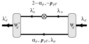
Figure 7: The deuteron matrix element of a one-body neutron operator (zero momentum transfer). The intermediate proton state has LF momentum $\alpha_{p}$ and $\bm{p}_{pT}$ and LF helicity $\lambda_{p}$; the neutron states have LF momentum $2-\alpha_{p}$ and $-\bm{p}_{pT}$, and helicities $\lambda_{n}$ and ${\lambda^{\prime}}_{\!\!n}$. The variables describing the intermediate state are integrated/summed over.

To evaluate the spin sums in Eq. (188), we substitute the deuteron LF wave functions by their representation as bilinear forms in LF bispinors, Eq. (158). The matrix element of the nucleon operator between neutron states can likewise be represented as a bilinear form

$$\langle n,p_{n},{\lambda^{\prime}}_{\!\!n}|O_{n}|n,p_{n},\lambda_{n}\rangle\;\;=\;\;\bar{u}_{\rm LF}(p_{n},{\lambda^{\prime}}_{\!\!n})\,\Gamma_{n}\,u_{\rm LF}(p_{n},\lambda_{n}),$$ (191)

where the bispinor matrix $\Gamma_{n}$ is specific to the operator and governs the dependence of the matrix element on the LF helicities ${\lambda^{\prime}}_{\!\!n}$ and $\lambda_{n}$. The summations over $\lambda_{p}$, ${\lambda^{\prime}}_{\!\!n}$, and $\lambda_{n}$ in Eq. (188) can then be carried out and give rise to the bispinor projectors [cf. Appendix A]

$$\sum_{\lambda_{p}}v_{\rm LF}(p_{p},\lambda_{p})\bar{v}_{\rm LF}(p_{p},\lambda_{n})\; =\;(p_{p}\gamma-m),$$ (192a)

$$\sum_{\lambda_{n}}u_{\rm LF}(p_{n},\lambda_{n})\bar{u}_{\rm LF}(p_{n},\lambda_{n})\; =\;(p_{n}\gamma+m)$$

(same for $${\lambda^{\prime}}_{\!\!n}$$). (192b)

The deuteron expectation value Eq. (187) is then obtained as a bispinor trace,

$$\langle O_{n}\rangle\; =\;\int\frac{d\alpha_{p}}{\alpha_{p}}\,d^{2}p_{pT}\;\frac{2\,\textrm{tr}[\Pi_{n}\Gamma_{n}]}{(2-\alpha_{p})^{2}},$$ (193a)

$$\Pi_{n}\; \equiv\;(\rho_{pn})^{\alpha\beta}(p_{n}\gamma+m)\Gamma_{\alpha}(p_{p}\gamma-m)\Gamma_{\beta}(p_{n}\gamma+m),$$ (193b)

$$(\rho_{pn})^{\alpha\beta}\; \equiv\;\langle\epsilon^{\alpha}_{pn}\epsilon^{\beta\ast}_{pn}\rangle\;=\;\sum_{{\lambda^{\prime}}_{\!\!d},\lambda_{d}}\rho_{d}(\lambda_{d},{\lambda^{\prime}}_{\!\!d})\epsilon^{\alpha}_{pn}(\lambda_{d})\epsilon^{\beta\ast}_{pn}({\lambda^{\prime}}_{\!\!d}).$$ (193c)

$\Pi_{n}$ in Eq. (193b) is a matrix in bispinor indices and represents the effective neutron spin density matrix in the deuteron for a given proton LF momentum $\alpha_{p}$ and $\bm{p}_{pT}$ [or equivalently, for a given neutron momentum Eq. (189)]. It depends covariantly on the neutron and proton 4-momenta, $p_{p}$ and $p_{n}$, and the parameters characterizing the deuteron polarization. It satisfies the conditions

$$(p_{n}\gamma-m)\Pi_{n}\;=\;0,\hskip 20.00003pt\Pi_{n}(p_{n}\gamma-m)\;=\;0.$$ (194)

which follow from the Dirac equation of the neutron bispinors. $\rho_{pn}$ in Eq. (193c) is the ensemble average of the $pn$ polarization vectors, Eq. (164), with the deuteron spin density matrix and represents the spin density matrix of the $pn$ configuration in the polarized deuteron in LF quantization. It depends covariantly on the total 4-momentum of the $pn$ system, $p_{pn}$, as well as on the axial 4-vector and 4-tensor characterizing the deuteron polarization, $s_{d}$ and $t_{d}$. It satisfies the conditions

$$p_{pn,\alpha}(\rho_{pn})^{\alpha\beta}\;=\;0,\hskip 20.00003pt(\rho_{pn})^{\alpha\beta}p_{pn,\beta}\;=\;0,$$ (195)

which follow from Eq. (164); they are analogous to those satisfied by the deuteron density matrix but involve the 4-momentum of the $pn$ system rather than that of the deuteron. Explicit expressions for $\Pi_{n}$ and $\rho_{pn}$ will be derived in the following.

The representation of the expectation value of Eq. (193a) has several important advantages: (a) The projectors resulting from the summation over the nucleon LF helicities, Eq. (192), do not “remember” the specific form of the LF helicity spinors; they are the same as for canonical spinors summed over the canonical spin. (In the 3-dimensional formulation of spin structure, this comes about because the Melosh rotations cancel when summing over the nucleon LF helicities; see Appendix A) This implies that the “knowledge” of the specific choice of the LF spin states resides only in the function $\Gamma^{\alpha}$, Eq. (167), and the spin density matrix of the $pn$ configuration, $\rho_{pn}$, Eq. (193c). (b) The covariant definition of $\rho_{pn}$ and $\Pi_{n}$ constrains their dependence on the proton and neutron 4-momenta and the deuteron polarization vector and tensor and greatly simplifies the calculation. (c) The neutron spin density matrix Eq. (193b) can be computed in closed form and has a simple structure. It can be compared with the density matrix of a free neutron, Eq. (5), and interpreted accordingly. (d) Products of gamma matrices and bispinor traces are easily evaluated. Equation (193a) will be our main tool in the subsequent deuteron structure calculations.

V.2 Neutron spin density matrix

We now evaluate the effective neutron spin density matrix in the polarized deuteron, Eq. (193b). We first derive explicit expressions for the spin density matrix of the $pn$ system, Eq. (193c), taking into account the properties of the LF spin wave functions Eq. (164) and the conditions Eq. (195). We then calculate the contraction in Eq. (193b) with these expressions and convert the result to a form that can be compared with the free neutron density matrix. We consider separately the contributions of the unpolarized, vector-polarized, and tensor-polarized parts of the deuteron spin density matrix, Eq. (16), to the neutron density matrix, Eq. (193b), and write

$$\Pi_{n}\; =\;\Pi_{n}[\textrm{unpol}]\,+\,\Pi_{n}[\textrm{vector}]\,+\,\Pi_{n}[\textrm{tensor}].$$ (196)

The unpolarized part of the $pn$ spin density matrix is given by

$$(\rho_{pn})^{\alpha\beta}[\textrm{unpol}]\;\;=\;\;\frac{1}{3}\left(-g^{\alpha\beta}+\frac{p_{pn}^{\alpha}p_{pn}^{\beta}}{M_{pn}^{2}}\right).$$ (197)

It corresponds to the general form of Eq. (17) but involves the 4-momentum of the $pn$ configuration instead of that of the deuteron, cf. Eq. (164). Substituting Eq. (197) in Eq. (193b), we obtain the effective neutron density matrix in the unpolarized as

$$\Pi_{n}[\textrm{unpol}]\;= \;\frac{1}{3}(p_{n}\gamma+m)\;\left[(12m^{2}-2\Delta^{2})G_{1}^{2}\right.$$

$$\left.-4m\Delta^{2}G_{1}G_{2}+(\Delta^{2})^{2}G_{2}^{2}\right]$$

$$[G_{1,2}\equiv G_{1,2}(M_{pn})].$$ (198)

The result has been simplified by making use of gamma matrix identities and the properties of the projectors Eq. (192). The effective neutron density matrix has the form of the density matrix of a free neutron with 4-momentum $p_{n}$, multiplied by a certain function of the invariant mass of the $pn$ pair, which is quadratic in the scalar functions $G_{1,2}$, Eq. (169).

The vector-polarized part of the $pn$ spin density matrix is given by

$$(\rho_{pn})^{\alpha\beta}[\textrm{vector}]\;\;=\;\;\frac{i}{2M_{pn}}\epsilon^{\alpha\beta\gamma\delta}p_{pn,\gamma}s_{pn,\delta}.$$ (199)

Here $s_{pn}$ is the polarization vector of the $pn$ configuration in the collinear frame,

$$s_{pn}\; \equiv\;\left[\frac{p_{d}^{+}}{M_{pn}}S_{d}^{z},\;-\frac{M_{pn}}{p_{d}^{+}}S_{d}^{z},\;\bm{S}_{dT}\right],$$ (200a)

$$(s_{pn}p_{pn})\; =\;0,$$ (200b)

$$s_{pn}^{2}\; =\;-(S_{d}^{z})^{2}-|\bm{S}_{dT}|^{2}\;=\;-|\bm{S}_{d}|^{2},$$ (200c)

where $S_{d}^{z}$ and $\bm{S}_{dT}$ are the components of the deuteron polarization vector in the rest frame,

$$\bm{S}_{d}\; =\;(\bm{S}_{dT},S_{d}^{z}),\hskip 20.00003pt|\bm{S}_{d}|^{2}\;\leq\;1.$$ (201)

Again the form of Eqs. (199) and (200) corresponds to that of the deuteron spin density matrix and polarization vector, cf. Eq. (131), only the quantities are constructed with the $pn$ 4-momentum rather than the deuteron 4-momentum. Substituting Eq. (199) in Eq. (193b), we obtain the effective neutron density matrix induced by deuteron vector polarization,

$$\Pi_{n}[\textrm{vector}]\; =\;{\textstyle\frac{1}{2}}(p_{n}\gamma+m)(s_{n}\gamma)\gamma^{5},$$ (202a)

$$s_{n}^{\alpha}\; =\;2M_{pn}\left(2mG_{1}a_{1}^{\alpha}-\Delta^{2}G_{2}a_{2}^{\alpha}\right)G_{1},$$ (202b)

$$a_{1}^{\alpha}\; =\;\left(g_{\alpha\beta}-\frac{p_{n,\alpha}p_{n,\beta}}{m^{2}}\right)s_{pn}^{\beta},$$ (202c)

$$a_{2}^{\alpha}\; =\;\left(g_{\alpha\beta}-\frac{\Delta_{\alpha}\Delta_{\beta}}{\Delta^{2}}\right)s_{pn}^{\beta},$$ (202d)

$$s_{n}p_{n}\; =\;0,\hskip 20.00003pta_{1}p_{n}=0,\hskip 20.00003pta_{2}p_{n}=0.$$ (202e)

The specific form of Eq. (202) is obtained by making extensive use of gamma matrix identities and the properties of the projectors Eqs. (192). The effective neutron density matrix Eq. (202a) depends on the axial vector $s_{n}$, Eq. (202b), which may be regarded as the effective polarization vector of the neutron in the deuteron. It is constructed from the the auxiliary 4-vectors $a_{1}$ and $a_{2}$, which are projections of the $pn$ polarization 4-vector $s_{pn}$ on the subspaces orthogonal to $p_{n}$ and $\Delta$. Note that the two structures in Eq. (202b) individually satisfy the condition $p_{n}s_{n}=0$ for any value of the scalar functions $G_{1}$ and $G_{2}$.

The tensor-polarized part of the $pn$ spin density matrix is parameterized as

$$(\rho_{pn})^{\alpha\beta}[\textrm{tensor}]\;=\;-(t_{pn})^{\alpha\beta},$$ (203)

where $t_{pn}$ is the polarization 4-tensor of the $pn$ configuration and satisfies

$$(t_{pn})^{\alpha\beta}\; =\;(t_{pn})^{\beta\alpha},\hskip 20.00003pt(t_{pn})^{\alpha}_{\;\;\alpha}\;=\;0,$$ (204a)

$$p_{pn,\alpha}(t_{pn})^{\alpha\beta}\; =\;(t_{pn})^{\alpha\beta}p_{pn,\beta}\;=\;0.$$ (204b)

The tensor can be constructed in analogy to the polarization 4-vector of Eq. (200). Its LF components in the collinear frame are [in the notation of Eq. (136)]

$$t_{pn}\; = \;\left[\begin{array}[]{rrr}\displaystyle\frac{(p_{d}^{+})^{2}}{M_{pn}^{2}}T_{d}^{zz}&-T_{d}^{zz}&\displaystyle\frac{p_{d}^{+}}{M_{pn}}T_{d}^{zj}\\[8.61108pt] -T_{d}^{zz}&\displaystyle\frac{M_{pn}^{2}}{(p_{d}^{+})^{2}}T_{d}^{zz}&\displaystyle-\frac{M_{pn}}{p_{d}^{+}}T_{d}^{zj}\\[8.61108pt] \displaystyle\frac{p_{d}^{+}}{M_{pn}}T_{d}^{zi}&\displaystyle-\frac{M_{pn}}{p_{d}^{+}}T_{d}^{zi}&T_{d}^{ij}\end{array}\right],$$ (208)

where $T_{d}^{zz},T_{d}^{zi}$ and $T_{d}^{ij}$ ($i,j=x,y$) are the components of is the deuteron polarization 3-tensor in the rest frame. The $pn$ tensor in Eq. (208) has the same form as the deuteron tensor, Eq. (140), only with the deuteron mass in the boost parameter replaced by the $pn$ invariant mass. Substituting Eq. (203) in Eq. (193b), the effective neutron density matrix induced by the deuteron tensor polarization is obtained as

$$\Pi_{n}[\textrm{tensor}]\; =\;\frac{1}{2}(p_{n}\gamma+m)\;(p_{n}t_{pn}p_{n})\;$$

$$\times\;8\left(G_{1}^{2}+\Delta^{2}G_{2}^{2}-4mG_{1}G_{2}\right).$$ (209)

One observes that the neutron density matrix induced by deuteron tensor polarization has has the same form as the unpolarized density matrix Eq. (198). The deuteron tensor polarization enters in the neutron density matrix only through the contraction $(p_{n}t_{pn}p_{n})$. This encodes the constraints from rotational and relativistic covariance. It implies that the tensor polarization of the deuteron cannot induce an effective spin polarization of the neutron. Altogether, Eq. (196), with the parts given by Eqs. (198), (202) and (209), describes the effective neutron spin density matrix in a polarized deuteron ensemble with general vector and tensor polarization,

The neutron spin density matrix becomes particularly simple when expressed in terms of the CM frame variables [see Sec. IV.3, Eq. (183)]. This representation allows one to identify the contributions of the S- and D-waves and relate the effective neutron polarization to 3-dimensional deuteron structure. The unpolarized part of the neutron density matrix, Eq. (198), becomes

$$\Pi_{n}[\textrm{unpol}] = \frac{1}{2}(p_{n}\gamma+m)(f_{0}^{2}+f_{2}^{2})$$ (210)

$$[f_{0,2}\equiv f_{0,2}(k)].$$

In the vector-polarized part, the $pn$ polarization 4-vector Eq. (200) is in the CM frame given by (we give both the LF and ordinary components, cf. Sec. IV.3)

$$s_{pn}[\textrm{CM}]\; = \;[S_{d}^{z},-S_{d}^{z},\bm{S}_{dT}]\;=\;(0,\bm{S}_{d}),$$ (211)

i.e., it has the same components as the deuteron polarization 4-vector in the deuteron rest frame. It is straightforward to compute the neutron polarization vector from the formulas in Eq. (202). The 4-vector products in Eq. (202c) and (202e) can be evaluated directly in the CM frame and become

$$s_{pn}p_{n}\; =\;s_{pn}[\textrm{CM}]\;p_{n}[\textrm{CM}]\;=\;\bm{S}_{d}\bm{k},$$ (212a)

$$s_{pn}\Delta\; =\;s_{pn}[\textrm{CM}]\;\Delta[\textrm{CM}]\;=\;-2\bm{S}_{d}\bm{k}.$$ (212b)

Altogether we obtain the vector-polarized part of the neutron spin density matrix in the CM frame as

$$\Pi_{n}[\textrm{vector}]\; =\;{\textstyle\frac{1}{2}}(p_{n}\gamma+m)(s_{n}\gamma)\gamma^{5},$$ (213a)

$$s_{n}[\textrm{CM}]\; =\;(s_{n}^{0},\bm{s}_{n}),$$ (213b)

$$s_{n}^{0}\; =\;-\frac{\bm{S}_{d}\bm{k}}{m}\left(f_{0}-\frac{f_{2}}{\sqrt{2}}\right)^{2},$$ (213c)

$$\bm{s}_{n}\; =\;\left[\left(\bm{S}_{d}+\frac{E-m}{m}\frac{(\bm{S}_{d}\bm{k})\bm{k}}{|\bm{k}|^{2}}\right)f_{0}\right.$$

$$+\;\left.\left(2\bm{S}_{d}-\frac{E+2m}{m}\frac{(\bm{S}_{d}\bm{k})\bm{k}}{|\bm{k}|^{2}}\right)\frac{f_{2}}{\sqrt{2}}\right]$$

$$\times\;\left(f_{0}-\frac{f_{2}}{\sqrt{2}}\right).$$ (213d)

The components of $s_{n}$ in an arbitrary collinear frame can be obtained from Eq. (213) by forming the LF plus and minus components in the CM frame, and performing a longitudinal boost to the desired value of $p_{d}^{+}$ (cf. Secs. III.8 and IV.3)

$$s_{n}^{\pm}[\textrm{CM}]\; =\;(s_{n}^{0}\,\pm\,s_{n}^{z})[\textrm{CM}],$$ (214a)

$$s_{n}^{+}[\textrm{arb.~{}coll.}]\; =\;\frac{p_{d}^{+}}{M_{pn}}\,s_{n}^{+}[\textrm{CM}],$$ (214b)

$$s_{n}^{-}[\textrm{arb.~{}coll.}]\; =\;\frac{M_{pn}}{p_{d}^{+}}\,s_{n}^{-}[\textrm{CM}],$$ (214c)

$$\bm{s}_{nT}[\textrm{arb.~{}coll.}]\; =\;\bm{s}_{nT}[\textrm{CM}].$$ (214d)

In the tensor-polarized part, the $pn$ polarization 4-tensor Eq. (203) is in the CM frame given by (we give the ordinary components)

$$(t_{pn})^{\alpha 0}[\textrm{CM}]\; =\;(t_{pn})^{0\beta}[\textrm{CM}]\;=\;0,$$ (215a)

$$(t_{pn})^{ij}[\textrm{CM}]\; =\;(T_{d})^{ij}\;\neq\;0,$$ (215b)

where $(T_{d})^{ij}$ are the components of the 3-dimensional deuteron polarization tensor in the deuteron rest frame. The contraction in Eq. (209) becomes

$$(p_{n}t_{pn}p_{n})\; = \;(\bm{k}T_{d}\bm{k}).$$ (216)

We obtain the tensor-polarized part of the neutron spin density matrix in the CM frame as

$$\Pi_{n}[\textrm{tensor}]\; =\;-\frac{1}{2}(p_{n}\gamma+m)\;\frac{3(\bm{k}T_{d}\bm{k})}{|\bm{k}|^{2}}$$

$$\times\;\left(2f_{0}+\frac{f_{2}}{\sqrt{2}}\right)\frac{f_{2}}{\sqrt{2}}.$$ (217)

Together, Eqs. (210), (213) and (217) specify the neutron spin density matrix in terms of the CM frame variables.

The structure of the neutron spin density matrix in terms of the CM frame variables shows several interesting features. (a) The unpolarized part, Eq. (210), is the sum of S- and D-wave probabilities of the CM wave function, as expected. (b) The vector-polarized part of the neutron spin density matrix, Eq. (213), involves mixing of the S- and D-waves. This is a consequence of the relativistic spin rotations involved in the transition from canonical spin states to LF helicity states (Melosh rotations; in our formulation they are contained in the explicit form of the LF helicity bispinors). (c) The tensor-polarized part of the neutron spin density matrix, Eq. (217), is proportional to the D-wave. This is natural, as tensor polarization would be absent for a pure S-wave bound state in the CM frame and cannot be induced by relativistic spin rotations ($|\Delta L|\leq 1$).

The neutron density matrix Eq. (196), with the parts given by Eqs. (198), (202) and (209), or equivalently by Eqs. (210), (213) and (217), contains the full information on the effective neutron polarization (longitudinal and transverse spin, spin-orbit correlations) in a general polarized deuteron ensemble. We use this density matrix to calculate the neutron LF helicity distributions in Sec. V.3 and the tagged DIS structure functions in Sec. VI

In the following applications we need the effective neutron spin density matrix in a pure deuteron spin state polarized along a given direction. It can be obtained by evaluating the general expressions for the neutron density matrix derived in this section, Eqs. (210), (213) and (217), with the specific values of the rest-frame polarization 3-vector and 3-tensor corresponding to the pure spin state given in Sec. II.2. For a state with spin projection $\lambda_{d}$ along a rest-frame direction $\bm{N}$, with $|\bm{N}|^{2}=1$, the neutron density is obtained as

$$\Pi_{n}[\textrm{pure}](\bm{N},\lambda_{d})\; =\;\Pi_{n}[\textrm{unpol}]\;+\;\Pi_{n}[\textrm{vector}](\bm{S}_{d})$$

$$+\;\Pi_{n}[\textrm{tensor}](T_{d})$$ (218a)

$$\bm{S}_{d}\; =\;\lambda_{d}\bm{N},$$ (218b)

$$T_{d}\; =\;-\frac{1}{6}\left(\delta^{ij}-3N^{i}N^{j}\right)$$

$$\times\;\left\{\begin{array}[]{rl}1,&\lambda_{d}=\pm 1\\ (-2),&\lambda_{d}=0\end{array}\right\},$$ (218e)

$$(\bm{k}T_{d}\bm{k})\; =\;-\frac{1}{6}\left[|\bm{k}|^{2}-3(\bm{N}\bm{k})^{2}\right]$$

$$\times\;\left\{\begin{array}[]{rl}1,&\lambda_{d}=\pm 1\\ (-2),&\lambda_{d}=0\end{array}\right\},$$ (218h)

where the general expressions of the terms in Eq. (218a) are given by Eqs. (210), (213) and (217). The 3-tensor of Eq. (218e) represents the rest-frame components of the special tensor Eq. (26).

V.3 Neutron light-front momentum distributions

We now want to calculate the LF momentum distributions of nucleons with given LF helicity in the deuteron. The simplest way is to calculate the expectation value of the plus component of the vector and axial vector current in the deuteron (i.e., the deuteron’s vector and axial charge) in the IA, and represent it as an integral over the LF momentum of the nucleons. A formal definition of the LF momentum distributions can be given using the second-quantized nucleon number operators or light-ray operators.

The expectation value of the isoscalar vector current in a deuteron ensemble is of the general form

$$\langle J_{V}^{+}\rangle\; = \;2p_{d}^{+}\,g^{\phantom{+}}_{Vd},$$ (219)

where $g_{Vd}=2$ is the vector charge (baryon number) of the deuteron. In the IA the current is the sum of the proton and neutron currents. The deuteron expectation value can be computed as the sum of the nucleon contributions, using the general formulas of Sec. V.1. The matrix element of the vector current between neutron states with LF helicity $\lambda_{n}=\pm 1/2$ is

$$\langle n,p_{n},{\lambda^{\prime}}_{\!\!n}|J_{V}^{+}|n,p_{n},\lambda_{n}\rangle$$

$$=\;\bar{u}_{\rm LF}(p_{n},{\lambda^{\prime}}_{\!\!n})\gamma^{+}u_{\rm LF}(p_{n},\lambda_{n})\;g_{V}$$ (220a)

$$=\;2p_{n}^{+}\delta(\lambda_{n},{\lambda^{\prime}}_{\!\!n})\;g_{V},$$ (220b)

where $g_{V}=1$ is the isoscalar vector charge of the nucleon. The matrix element is diagonal in the LF helicities and independent of their value. The vector current thus “counts” the helicity-independent (or averaged) number of neutrons. According to Eq. (193a) the neutron contribution to the deuteron expectation value is given by

$$\langle J_{V}^{+}\rangle\; =\;g_{V}\int\frac{d\alpha_{p}}{\alpha_{p}}\,d^{2}p_{pT}\;\frac{2\;\textrm{tr}[\Pi_{n}\gamma^{+}]}{(2-\alpha_{p})^{2}}$$

$$=\;p_{d}^{+}\,g_{Vd}.$$ (221)

We identify the function

$$\mathcal{S}_{d}(\alpha_{p},\bm{p}_{pT})\; \equiv \;\frac{\textrm{tr}[\Pi_{n}\gamma^{+}]}{(2-\alpha_{p})^{2}\;p_{d}^{+}}$$ (222)

as the helicity-independent LF momentum distribution of neutrons in the deuteron ensemble. In accordance with nuclear physics terminology we refer to it as the deuteron LF spectral function (see explanation below). It is a function of the proton LF momentum variables and satisfies

$$\int\frac{d\alpha_{p}}{\alpha_{p}}\,d^{2}p_{pT}\;\mathcal{S}_{d}(\alpha_{p},\bm{p}_{pT})\; = \;\frac{g_{Vd}}{2g_{V}}\;=\;1.$$ (223)

The trace in Eq. (222) receives contributions from the unpolarized and tensor-polarized parts of the neutron density matrix. Substituting the explicit form of the neutron density matrix in the CM frame variable, Eqs. (210) and (217), and using

$$\frac{1}{2}{\rm tr}[(p_{n}\gamma+m)\gamma^{+}]\; = \;2p_{n}^{+}\;=\;(2-\alpha_{p})p_{d}^{+}$$ (224)

we obtain

$$\mathcal{S}_{d}\; =\;\mathcal{S}_{d}[\textrm{unpol}]\;+\;\mathcal{S}_{d}[\textrm{tensor}],$$ (225a)

$$\mathcal{S}_{d}(\alpha_{p},\bm{p}_{pT})[\textrm{unpol}]\; =\;\frac{f_{0}^{2}+f_{2}^{2}}{2-\alpha_{p}},$$ (225b)

$$\mathcal{S}_{d}(\alpha_{p},\bm{p}_{pT})[\textrm{tensor}]\; =\;-\frac{3}{2-\alpha_{p}}\;\frac{(\bm{k}T_{d}\bm{k})}{|\bm{k}|^{2}}$$

$$\times\;\left(2f_{0}+\frac{f_{2}}{\sqrt{2}}\right)\frac{f_{2}}{\sqrt{2}}.$$ (225c)

The LF momentum-dependent prefactor could equivalently be expressed in terms of the CM momentum variable as

$$\frac{1}{2-\alpha_{p}}\;=\;\frac{E}{E-k^{z}};$$ (226)

we leave it in its original form, as in this form it can be combined with similar factors appearing in integrals over the LF momentum. Using the relation Eq. (179) one easily verifies that the unpolarized part Eq. (225b) satisfies the normalization condition Eq. (223), and that the tensor-polarized part Eq. (225c) averages to zero,

$$\int\frac{d\alpha_{p}}{\alpha_{p}}\,d^{2}p_{pT}\;\mathcal{S}_{d}(\alpha_{p},\bm{p}_{pT})[\textrm{unpol}]$$

$$=\;\int\frac{d^{3}k}{E}\;(f_{0}^{2}+f_{2}^{2})\;=\;1,$$ (227a)

$$\int\frac{d\alpha_{p}}{\alpha_{p}}\,d^{2}p_{pT}\;\mathcal{S}_{d}(\alpha_{p},\bm{p}_{pT})[\textrm{tensor}]$$

$$\propto\;\int d\Omega_{k}\frac{(\bm{k}T_{d}\bm{k})}{|\bm{k}|^{2}}\;=\;0.$$ (227b)

Eq. (227b) holds because the polarization tensor in the CM frame is traceless, cf. Eq. (215). These relations ensure the conservation of baryon number in the deuteron LF structure.

The helicity-independent neutron distributions also satisfy a LF momentum sum rule. Because the functions

$$\frac{\mathcal{S}_{d}(\alpha_{p},\bm{p}_{pT})}{\alpha_{p}}[\textrm{unpol}]\hskip 10.00002pt\textrm{and}\hskip 10.00002pt\frac{\mathcal{S}_{d}(\alpha_{p},\bm{p}_{pT})}{\alpha_{p}}[\textrm{tensor}]$$ (228)

are symmetric under $\alpha_{p}\rightarrow 2-\alpha_{p}$, Eqs. (227a) and (227b) imply

$$\int\frac{d\alpha_{p}}{\alpha_{p}}\,d^{2}p_{pT}\;(2-\alpha_{p})\;\mathcal{S}_{d}(\alpha_{p},\bm{p}_{pT})[\textrm{unpol}]\; =\;1,$$ (229a)

$$\int\frac{d\alpha_{p}}{\alpha_{p}}\,d^{2}p_{pT}\;(2-\alpha_{p})\;\mathcal{S}_{d}(\alpha_{p},\bm{p}_{pT})[\textrm{tensor}]\; =\;0.$$ (229b)

This relation ensures LF momentum conservation in tagged DIS on the deuteron (see Sec. VI).

In a similar way we can obtain the spin-dependent neutron LF momentum distribution in a vector-polarized deuteron. The expectation value of the isoscalar axial vector current in the deuteron ensemble is

$$\langle J_{A}^{+}\rangle\; = \;2M_{d}s_{d}^{+}\,g_{Ad}\;\;=\;\;2S_{d}^{z}\,p_{d}^{+}\,g_{Ad},$$ (230)

where we used the explicit form of polarization vector in collinear frame, Eq. (131). Here $g_{Ad}$ is the axial charge of the deuteron, which is a property of the deuteron bound state and cannot be determined from first principles. The axial current is the sum of proton and neutron currents. The matrix element of the neutron axial current between nucleon states with LF helicity $\lambda_{n}=\pm 1/2$ is

$$\langle n,p_{n},{\lambda^{\prime}}_{\!\!n}|J_{A}^{+}|n,p_{n},\lambda_{n}\rangle$$

$$=\;\bar{u}_{\rm LF}(p_{n},{\lambda^{\prime}}_{\!\!n})(-\gamma^{+}\gamma^{5})u_{\rm LF}(p_{n},\lambda_{n})\,g_{A}$$ (231a)

$$=\;2p_{n}^{+}\;(2\lambda_{n})\,\delta(\lambda_{n},{\lambda^{\prime}}_{\!\!n})\,g_{A},$$ (231b)

where $g_{A}$ is the isoscalar axial coupling of the nucleon. The matrix element is again diagonal in the LF helicities, but the diagonal value is now proportional to the LF helicity. The axial vector current with matrix $-\gamma^{+}\gamma^{5}$ therefore counts the difference between the number of neutrons with LF helicities $+1/2$ and $-1/2$. The calculation of the deuteron expectation value proceeds analogously to Eq. (221), and we identify

$$\Delta\mathcal{S}_{d}(\alpha_{p},\bm{p}_{pT})\; \equiv \;\frac{\textrm{tr}[\Pi_{n}(-\gamma^{+}\gamma^{5})]}{(2-\alpha_{p})^{2}\;p_{d}^{+}}$$ (232)

as the helicity-dependent LF momentum distribution of neutrons in the deuteron ensemble. It satisfies

$$\int\frac{d\alpha_{p}}{\alpha_{p}}\,d^{2}p_{pT}\;\Delta\mathcal{S}_{d}(\alpha_{p},\bm{p}_{pT})\; = \;S_{d}^{z}\,\left(\frac{g_{Ad}}{2g_{A}}\right),$$ (233)

which may be regarded as the nucleon spin sum rule. Only the vector-polarized part of the neutron density matrix Eq. (196) contributes to the trace in Eq. (232),

$$\Delta\mathcal{S}_{d}\; \equiv \;\Delta\mathcal{S}_{d}[\textrm{vector}].$$ (234)

With Eq. (213) we obtain

$$\textrm{tr}[\Pi_{n}(-\gamma^{+}\gamma^{5})]\; =\frac{1}{2}{\rm tr}[(p_{n}\gamma+m)(s_{n}\gamma)\gamma^{5}(-\gamma^{+}\gamma^{5})]$$

$$=\;2ms_{n}^{+}.$$ (235)

Using the explicit expressions for the neutron polarization vector in the CM frame, Eq. (213), we obtain

$$\Delta\mathcal{S}_{d}(\alpha_{p},\bm{p}_{pT})\; =\;\frac{1}{2-\alpha_{p}}\;\left(f_{0}-\frac{f_{2}}{\sqrt{2}}\right)$$

$$\times\;\left(C_{0}f_{0}-\frac{C_{2}f_{2}}{\sqrt{2}}\right),$$ (236)

where

$$C_{0} \equiv C_{0}(\bm{k})$$

$$\equiv\frac{m}{(2-\alpha_{p})E}\left[S_{d}^{z}\;-\;\frac{\bm{S}_{d}\bm{k}}{m}\;+\;\frac{(\bm{S}_{d}\bm{k})k^{z}}{m(E+m)}\right],$$ (237a)

$$C_{2} \equiv C_{2}(\bm{k})$$

$$\equiv\frac{m}{(2-\alpha_{p})E}\left[-2S_{d}^{z}-\frac{\bm{S}_{d}\bm{k}}{m}+\frac{(E+2m)\,(\bm{S}_{d}\bm{k})k^{z}}{m|\bm{k}|^{2}}\right].$$ (237b)

These factors can also be written in the form

$$C_{0}(\bm{k}) =\;S_{d}^{z}-\frac{(E+k^{z})|\bm{k}_{T}|^{2}}{(E+m)(m^{2}+|\bm{k}_{T}|^{2})}\,S_{d}^{z}$$

$$-\frac{(E+k^{z})(E-k^{z}+m)}{(E+m)(m^{2}+|\bm{k}_{T}|^{2})}\,(\bm{S}_{dT}\bm{k}_{T}),$$ (238a)

$$C_{2}(\bm{k}) =\;S_{d}^{z}-\frac{(E+2m)(E+k^{z})|\bm{k}_{T}|^{2}}{(m^{2}+|\bm{k}_{T}|^{2})|\bm{k}|^{2}}\,S_{d}^{z}$$

$$+\;\frac{(E+k^{z})[-|\bm{k}|^{2}+(E+2m)k^{z}]}{(m^{2}+|\bm{k}_{T}|^{2})|\bm{k}|^{2}}\,(\bm{S}_{dT}\bm{k}_{T}),$$ (238b)

where we have used that

$$(E+k^{z})(E-k^{z})\; =\;E^{2}-(k^{z})^{2}$$

$$=\;m^{2}+|\bm{k}_{T}|^{2},$$ (239a)

$$2-\alpha_{p}\; =\;1-\frac{k^{z}}{E},$$ (239b)

$$\frac{1}{2-\alpha_{p}}\; =\;\frac{E}{E-k^{z}}\;=\;\frac{E(E+k^{z})}{m^{2}+|\bm{k}_{T}|^{2}}.$$ (239c)

The factors $C_{0}$ and $C_{2}$ describe the effect of the nucleons’ orbital motion on the neutron LF helicity. In the 3-dimensional representation of the deuteron LF wave function they arise from the Melosh rotations connecting the canonical nucleon spinors with the LF helicity spinors (see Appendix B). In the 4-dimensional representation employed here this information is encoded in the specific form of the effective neutron polarization vector $s_{n}$, Eq. (202b). Note that the factors are equal to unity at zero transverse momentum, cf. Eqs. (238a) and (238b),

$$C_{0}(\bm{k}),C_{2}(\bm{k})\;=\;1\hskip 10.00002pt\textrm{at}\hskip 10.00002pt\bm{k}_{T}=\bm{p}_{pT}=0,\;k^{z}\;\textrm{arbitrary},$$ (240)

as is expected of the Melosh rotation.

In the CM representation Eq. (236) one can easily evaluate the normalization integral of the polarized nucleon distribution, Eq. (233). Using the relation Eq. (179) one obtains

$$\left(\frac{g_{Ad}}{2g_{A}}\right)\,S_{d}^{z}$$

$$=\;\int\frac{d\alpha_{p}}{\alpha_{p}}\,d^{2}p_{pT}\Delta\mathcal{S}_{d}(\alpha_{p},\bm{p}_{pT})$$

$$=\;\int\frac{d^{3}k}{E}\;\left(f_{0}-\frac{f_{2}}{\sqrt{2}}\right)\left(C_{0}f_{0}-\frac{C_{2}f_{2}}{\sqrt{2}}\right)$$

$$=\;4\pi\int\frac{dk\;k^{2}}{E}\;\left(f_{0}-\frac{f_{2}}{\sqrt{2}}\right)\left(\bar{C}_{0}f_{0}-\frac{\bar{C}_{2}f_{2}}{\sqrt{2}}\right),$$ (241)

where $\bar{C}_{0},\bar{C}_{2}$ are the angular averages of the factors $C_{0},C_{2}$,

$$\bar{C}_{0}(k)\; \equiv\;\int\frac{d\Omega_{k}}{4\pi}\;C_{0}(\bm{k})$$

$$=\;\frac{m\,S_{d}^{z}}{E+m}\left(\frac{m}{k}\log\frac{E+k}{m}+1\right),$$ (242a)

$$\bar{C}_{2}(k)\; \equiv\;\int\frac{d\Omega_{k}}{4\pi}\;C_{2}(\bm{k})$$

$$=\;\frac{m\,S_{d}^{z}}{k^{2}}\left[(E+2m)\frac{m}{k}\log\frac{E+k}{m}-2E-m\right].$$ (242b)

Notice that structures proportional to $\bm{S}_{dT}\bm{k}_{T}$ average to zero, so that the averages are proportional to $S_{d}^{z}$, as it should be. The expansion in $k/m$ of the averages is

$$\bar{C}_{0}(k)\; =\;S_{d}^{z}\,\left[\phantom{-}1\;-\;\frac{1}{3}\frac{k^{2}}{m^{2}}\;+\;\mathcal{O}\left(\frac{k^{4}}{m^{4}}\right)\right],$$ (243a)

$$\bar{C}_{2}(k) =\;S_{d}^{z}\,\left[-1\;+\;\frac{4}{15}\frac{k^{2}}{m^{2}}\;+\;\mathcal{O}\left(\frac{k^{4}}{m^{4}}\right)\right].$$ (243b)

Neglecting terms $\mathcal{O}(k^{2}/m^{2})$, the integral Eq. (241) becomes

$$\frac{g_{Ad}}{2g_{A}}\; =\;4\pi\int\frac{dk\;k^{2}}{E}\;\left(f_{0}-\frac{f_{2}}{\sqrt{2}}\right)\left(f_{0}+\frac{f_{2}}{\sqrt{2}}\right)$$

$$=\;4\pi\int\frac{dk\;k^{2}}{E}\;\left(f_{0}^{2}-\frac{f_{2}^{2}}{2}\right)$$

$$=\;4\pi\int\frac{dk\;k^{2}}{E}\;\left(f_{0}^{2}+f_{2}^{2}-\frac{3f_{2}^{2}}{2}\right)$$

$$=\;1-\frac{3}{2}\omega_{2},$$ (244)

where we have canceled the factor $S_{d}^{z}$ on both sides. Here

$$\omega_{2}\;\equiv\;4\pi\int\frac{dk\,k^{2}}{E(k)}\;f_{2}^{2}(k)$$ (245)

is the D-state probability of the deuteron wave function in the CM frame. Equation (244) has the same form as the nonrelativistic result for the deuteron axial charge including the D-state correction.

Some explanations are in order regarding the definition of the LF spectral function and the correspondence with nuclear physics terminology. (a) The deuteron spectral function $\mathcal{S}_{d}$ describes the LF momentum distribution of neutrons in the deuteron as a function of the proton LF momentum and is normalized as Eq. (223); this definition is appropriate for tagged DIS experiments where the proton momentum is measured and will be used in the following. The conventional neutron LF momentum density is defined as a function of the neutron LF momentum and related to the spectral function as

$$\mathcal{N}_{d}(\alpha_{n},\bm{p}_{nT})\;= \;\frac{\alpha_{n}}{\alpha_{p}}\mathcal{S}_{d}(\alpha_{p},\bm{p}_{pT})\,$$

$$\;[\alpha_{p}=2-\alpha_{n},\;\bm{p}_{pT}=-\bm{p}_{nT}],$$ (246)

such that its normalization is

$$\int\frac{d\alpha_{n}}{\alpha_{n}}\int d^{2}p_{nT}\;\mathcal{N}_{d}(\alpha_{n},\bm{p}_{nT})\; =\;1.$$ (247)

(b) The spectral function represents the nuclear structure information entering in the IA. In the general case of a nucleus with $A>2$, it describes the probability density for removing a nucleon with a given momentum, while leaving the $A-1$ remnant system with a given excitation energy (the momentum of the $A-1$ system is fixed by the removed nucleon momentum) Benhar et al. (2005). The nucleon momentum density is then obtained by integrating over the excitation energy of the $A-1$ system. In the particular case of the deuteron with $A=2$, the remnant system is the single spectator nucleon, whose energy is fixed by the momentum, so that the spectral function depends on the momentum variable only and coincides with the momentum density up to a factor accounting for the normalization, cf. Eq. (247).

V.4 Distribution in unpolarized deuteron

The expressions Eqs. (225) and (236) describe the LF momentum distributions of neutrons in a deuteron ensemble with arbitrary polarization (vector, tensor). It is instructive to consider the distributions in some special cases. In an unpolarized ensemble ($\bm{S}=0,T=0$) only the helicity-independent neutron distribution Eqs. (225b) is present,

$$\mathcal{S}_{d}(\alpha_{p},\bm{p}_{pT})\; =\;\frac{f_{0}^{2}+f_{2}^{2}}{2-\alpha_{p}},$$ (248a)

$$\Delta\mathcal{S}_{d}(\alpha_{p},\bm{p}_{pT})\; =\;0.$$ (248b)

One notes that (a) in the helicity-independent distribution the S- and D-waves of the CM-frame wave function do not mix; (b) the helicity-dependent distribution is zero for arbitrary neutron LF momentum, i.e., no LF helicity polarization is induced by the orbital motion.

Figure 8: The deuteron spectral function $\mathcal{S}_{d}$ in the unpolarized deuteron, Eq. (248a). It describes the helicity-independent LF momentum distribution of neutrons in the unpolarized deuteron as a function of the proton LF momentum. The plot shows the dependence on $\alpha_{p}$ for several values of $|\bm{p}_{pT}|$.

Figure 8 shows the helicity-independent neutron distribution in the unpolarized deuteron as a function of $\alpha_{p}$ for several values of $|\bm{p}_{pT}|$. One observes: (a) The distribution is maximal at $\alpha_{p}=1$ and $|\bm{p}_{pT}|=0$ and drops steeply when increasing $|\alpha_{p}-1|$ or $|\bm{p}_{pT}|$, as implied by the nucleon momentum distribution in the CM frame. (b) An asymmetry between the distributions at $\alpha_{p}>1$ and $<1$ is caused by the flux factor $1/(2-\alpha_{p})$ in Eq. (248a). Figure 9 shows the ratio of the neutron distribution resulting from the D-wave only to that resulting from S- and D-waves (i.e., the total distribution),

$$\frac{\mathcal{S}_{d}(\alpha_{p},\bm{p}_{pT})\,[\textrm{D-wave}]}{\mathcal{S}_{d}(\alpha_{p},\bm{p}_{pT})\,[\textrm{S+D-waves}]}.$$ (249)

This ratio can be regarded the probability for sampling the D-wave component of the CM motion when observing a proton (or neutron) with given LF momentum. One observes: (a) The D-wave probability vanishes at $\alpha_{p}=1$ and $|\bm{p}_{pT}|=0$, corresponding to CM momentum $|\bm{k}|=0$. (b) The D-wave probability becomes unity at LF momenta corresponding to $|\bm{k}|\approx$ 400 MeV, where the S-wave function in the CM frame goes through zero Wiringa et al. (1995); (c) The D-wave probability decreases again at large CM momenta.

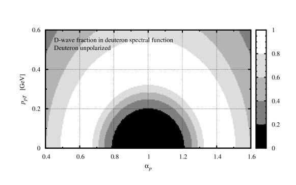
Figure 9: The D-wave fraction in the deuteron spectral function, $\mathcal{S}_{d}[\textrm{D-wave}]/\mathcal{S}_{d}[\textrm{S+D-waves}]$, in the unpolarized deuteron, Eq. (249). The 2-dimensional plot shows the ratio as a function of $\alpha_{p}$ and $|\bm{p}_{pT}|$.

V.5 Distribution in deuteron helicity states

In a pure deuteron state with LF helicity $+1$ the helicity-independent neutron distribution is

$$\mathcal{S}_{d}(\alpha_{p},\bm{p}_{pT})[\textrm{pure $+1$}]\; =\;\mathcal{S}_{d}(\alpha_{p},\bm{p}_{pT})[\textrm{unpol}]$$

$$+\;\mathcal{S}_{d}(\alpha_{p},\bm{p}_{pT})[\textrm{tensor}].$$ (250)

Here the tensor-polarized part is given by Eq. (225c), evaluated with the special tensor Eq. (218e), and with the contraction given by Eq. (218h), for polarization along the $z$-direction, $\bm{N}=\bm{e}_{z}$,

$$\mathcal{S}_{d}(\alpha_{p},\bm{p}_{pT})[\textrm{tensor}]$$

$$=\;-\frac{1}{2-\alpha_{p}}C_{T}\left(2f_{0}+\frac{f_{2}}{\sqrt{2}}\right)\frac{f_{2}}{\sqrt{2}},$$ (251a)

$$C_{T}\; \equiv\;C_{T}(\bm{k})\;=\;3\;\frac{(\bm{k}T\bm{k})}{|\bm{k}|^{2}}\;=\;\frac{1}{2}\left[-1+\frac{3(k^{z})^{2}}{|\bm{k}|^{2}}\right]$$

$$=\;1-\frac{3|\bm{k}_{T}|^{2}}{2|\bm{k}|^{2}}.$$ (251b)

Combining this with the unpolarized part given by Eq. (225b), we obtain

$$\mathcal{S}_{d}(\alpha_{p},\bm{p}_{pT})[\textrm{pure $+1$}]\;$$

$$=\;\frac{1}{2-\alpha_{p}}\left[f_{0}^{2}+f_{2}^{2}-C_{T}\left(2f_{0}+\frac{f_{2}}{\sqrt{2}}\right)\frac{f_{2}}{\sqrt{2}}\right].$$ (252)

The helicity-dependent neutron distribution is

$$\Delta\mathcal{S}_{d}(\alpha_{p},\bm{p}_{pT})[\textrm{pure $+1$}]$$

$$=\;\frac{1}{2-\alpha_{p}}\;\left(f_{0}-\frac{f_{2}}{\sqrt{2}}\right)\left(C_{0}f_{0}-\frac{C_{2}f_{2}}{\sqrt{2}}\right),$$ (253)

where $C_{0},C_{2}$ are the factors of Eqs. (237a) and (237b) with $S_{d}^{z}=1$ and $\bm{S}_{dT}=0$

$$C_{0} \equiv C_{0}(\bm{k})$$

$$\equiv\;\frac{m}{(2-\alpha_{p})E}\left[1\;-\;\frac{k^{z}}{m}\;+\;\frac{(k^{z})^{2}}{m(E+m)}\right],$$ (254a)

$$C_{2} \equiv C_{2}(\bm{k})$$

$$\equiv\;\frac{m}{(2-\alpha_{p})E}\left[-2\;-\;\frac{k^{z}}{m}\;+\;\frac{(E+2m)\,(k^{z})^{2}}{m|\bm{k}|^{2}}\right],$$ (254b)

which can also be written in the form

$$C_{0}(\bm{k})\; =\;1-\frac{(E+k^{z})|\bm{k}_{T}|^{2}}{(E+m)(m^{2}+|\bm{k}_{T}|^{2})},$$ (255a)

$$C_{2}(\bm{k})\; =\;1-\frac{(E+2m)(E+k^{z})|\bm{k}_{T}|^{2}}{(m^{2}+|\bm{k}_{T}|^{2})|\bm{k}|^{2}}.$$ (255b)

One may also consider the distributions of neutrons with LF helicity $+1/2$ and $-1/2$ in the deuteron state with LF helicity $+1$,

$$\mathcal{S}_{d\pm}[\textrm{pure $+1$}]\;\equiv\;\frac{1}{2}\left(\mathcal{S}_{d}\pm\Delta\mathcal{S}_{d}\right)[\textrm{pure $+1$}],$$ (256a)

$$\{\mathcal{S}_{d},\,\Delta\mathcal{S}_{d}\}[\textrm{pure $+1$}]\;=\;\left(\mathcal{S}_{d+}\pm\mathcal{S}_{d-}\right)[\textrm{pure $+1$}].$$ (256b)

The functions $S_{d\pm}$ are positive for arbitrary LF momenta

$$\mathcal{S}_{d\pm}\;\geq\;0,\hskip 20.00003pt|\Delta\mathcal{S}_{d}|\;\leq\;\mathcal{S}_{d}.$$ (257)

The positivity can be proved using the explicit expressions given above and will be demonstrated by the numerical results below. The functions $S_{d\pm}$ have a probabilistic interpretation as the distributions of neutrons with helicities “along” or “against” the deuteron helicity.

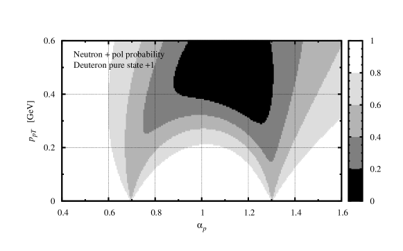
Figure 10: The deuteron spectral function ratio $\mathcal{S}_{d+}/(\mathcal{S}_{d+}+\mathcal{S}_{d-})$, Eq. (259), in the pure deuteron spin state with LF helicity $+1$. It describes the probability that a neutron observed at the given LF momentum has LF helicity $+1/2$, i.e., is polarized along the deuteron spin direction. The 2-dimensional plot shows the ratio as a function of $\alpha_{p}$ and $|\bm{p}_{pT}|$.

The effective polarization of the neutron in the deuteron depends on the proton LF momentum. An interesting effect is observed at zero transverse momentum, $\bm{p}_{pT}=\bm{k}_{T}=0$, and arbitrary longitudinal momentum $\alpha_{p}\neq 1,k^{z}\neq 0$. In this kinematic limit the factors $C_{0}$ and $C_{2}$ in $\Delta\mathcal{S}_{d}$ are unity, Eqs. (255a) and (255b), and the factor $C_{T}$ in $\mathcal{S}_{d}$ is also unity, Eq. (251b). The distributions Eq. (252) thus become

$$\mathcal{S}_{d}(\alpha_{p},\bm{p}_{pT}=0)[\textrm{pure $+1$}]$$

$$=\;\Delta\mathcal{S}_{d}(\alpha_{p},\bm{p}_{pT}=0)[\textrm{pure $+1$}]$$

$$=\;\mathcal{S}_{d+}(\alpha_{p},\bm{p}_{pT}=0)[\textrm{pure $+1$}]$$

$$=\;\frac{1}{2-\alpha_{p}}\left(f_{0}-\frac{f_{2}}{\sqrt{2}}\right)^{2},$$ (258a)

$$\mathcal{S}_{d-}(\alpha_{p},\bm{p}_{pT}=0)[\textrm{pure $+1$}]\;=\;0,$$ (258b)

and the neutron is completely polarized along the direction of the deuteron LF helicity. This happens because configurations with neutron LF helicity opposite to the deuteron involve LF orbital angular momentum $L_{z}\neq 0$, which requires non-zero transverse momentum. It is remarkable that the 4-dimensional representation of the deuteron LF wave function reproduces this effect without explicit reference to orbital angular momentum states. Notice that the distribution at $\bm{p}_{pT}$ includes contributions from the S- and D-wave of the CM wave function.

Figure 10 shows the ratio

$$\frac{\mathcal{S}_{d+}}{\mathcal{S}_{d+}+\mathcal{S}_{d-}}\;=\;\frac{1}{2}\left(1+\frac{\Delta\mathcal{S}_{d}}{\mathcal{S}_{d}}\right),\hskip 10.00002pt0\leq(\textrm{ratio})\leq 1,$$ (259)

in a pure deuteron spin state with LF helicity $+1$. It describes the probability that a neutron observed at a given LF momentum has LF helicity $+1/2$ (along the deuteron spin direction); the probability that it has LF helicity $-1/2$ (opposite to the deuteron spin direction) is given by 1 minus the ratio. The dependence on the LF momentum shows several interesting features: (a) The ratio is close to unity in the region $0.8<\alpha_{p}<1.2$ and $|\bm{p}_{pT}|<$ 200 MeV, which corresponds to CM momenta $|\bm{k}|\lesssim$ 200 MeV, where the S-wave dominates in the CM wave function. (b) The ratio is equal to unity at $|\bm{p}_{pT}|=0$ for arbitrary $\alpha_{p}$, as implied by Eq. (258). Exceptions are the points $\alpha_{p}=0.7$ and 1.3, which correspond to values of $k$ at which the combination of radial wave functions $(f_{0}-f_{2}/\sqrt{2})$ in Eq. (258) vanishes (singular points). (c) The ratio becomes small at $\alpha_{p}\sim 1$ and $|\bm{p}_{pT}|\geq$ 400 MeV. In this region the D-wave dominates in the CM wave function, and the effects of relativistic spin rotations are large.

In sum, one sees that the neutron polarization in the polarized deuteron can effectively be controlled by selecting certain regions of the LF momentum. This feature can be exploited in tagged DIS experiments (see below) and represents an important advantage of spectator tagging.

The integrals of the deuteron spectral functions over the proton transverse momentum $\bm{p}_{pT}$ describe the distributions of neutrons with respect to the longitudinal LF momentum fraction $\alpha_{p}$ only,

$$\mathcal{S}_{d}(\alpha_{p})\; \equiv\;\int d^{2}p_{pT}\;\mathcal{S}_{d}(\alpha_{p},\bm{p}_{pT}),$$ (260a)

$$\Delta\mathcal{S}_{d}(\alpha_{p})\; \equiv\;\int d^{2}p_{pT}\;\Delta\mathcal{S}_{d}(\alpha_{p},\bm{p}_{pT}),$$ (260b)

which are normalized such that

$$\int_{0}^{2}\frac{d\alpha_{p}}{\alpha_{p}}\;\left\{\mathcal{S}_{d}(\alpha_{p}),\,\Delta\mathcal{S}_{d}(\alpha_{p})\right\}\; = \;\left\{1,\,\frac{g_{Ad}}{2g_{A}}\right\}.$$ (261)

These functions are the analog of the parton distributions in the parton model of hadron structure and appear in the description of $\bm{p}_{pT}$-integrated tagged DIS measurements on the deuteron. Figures 11 and 12 show the integrated LF momentum densities obtained with our deuteron LF wave function. One observes: (a) The integrated distributions are concentrated in the region $\alpha_{p}\approx(0.9,1.1)$, corresponding to nucleon CM momenta $k\lesssim$ 100 MeV. (b) The neutrons are overwhelmingly polarized along the direction of the deuteron LF helicity. The integrated distribution $\mathcal{S}_{d-}$ is at the level of a few percent of $\mathcal{S}_{d+}$. The magnitude of the distribution is consistent with their normalization integrals: in the nonrelativistic limit, using Eq. (244), we find

$$\left.\left[\int\frac{d\alpha_{p}}{\alpha_{p}}\mathcal{S}_{d-}(\alpha_{p})\right]\right/\left[\int\frac{d\alpha_{p}}{\alpha_{p}}\mathcal{S}_{d+}(\alpha_{p})\right]\;\;\approx\;\;\frac{3}{4}\omega_{2}.$$ (262)

Figure 11: The deuteron spectral functions $\mathcal{S}_{d}$ and $\Delta\mathcal{S}_{d}$, integrated over the proton transverse momentum, in the pure deuteron spin state with LF helicity $+1$. These functions describe the helicity-independent and helicity-dependent LF momentum distributions of neutrons in the deuteron with LF helicity $+1$.

Figure 12: The deuteron spectral functions $\mathcal{S}_{d+}$ and $\Delta\mathcal{S}_{d-}$, integrated over the proton transverse momentum, in the pure deuteron spin state with LF helicity $+1$ (cf. Fig. 11). These functions describe the LF momentum distributions of neutrons with LF helicity $+1/2$ and $-1/2$ in the deuteron with LF helicity $+1$. The plot shows $\mathcal{S}_{d-}$ multiplied by 10.

VI Tagged DIS in impulse approximation

VI.1 Impulse approximation

We now calculate the cross section of polarized tagged DIS on the deuteron, using the LF methods developed in Secs. IV and V. We restrict ourselves to the IA, where it is assumed that (i) the current operator couples only to a single nucleon; (ii) the DIS final state produced from the active nucleon evolves independently from spectator. The IA result contains the nucleon pole and dominates the tagged DIS cross section at small proton momenta. The justification of the IA and steps of calculation are described in Ref. Strikman and Weiss (2018). Here we focus on the aspects specific to electron and deuteron polarization.

In tagged DIS on the deuteron in a general ensemble of spin states, described by the density matrix $\rho_{d}(\lambda_{d},{\lambda^{\prime}}_{\!\!d})$, the deuteron tensor given by

$$W_{d}^{\mu\nu}(p_{d},q,p_{p})\;=\;\langle W_{d}^{\mu\nu}\rangle$$

$$=\;\sum_{{\lambda^{\prime}}_{\!\!d},\lambda_{d}}\rho_{d}(\lambda_{d},{\lambda^{\prime}}_{\!\!d})\;W_{d}^{\mu\nu}(p_{d},q,p_{p}|{\lambda^{\prime}}_{\!\!d},\lambda_{d}),$$ (263)

where the tensor on the right-hand side is the nondiagonal deuteron tensor between LF helicity states with $\lambda_{d}$ and ${\lambda^{\prime}}_{\!\!d}$, cf. Eqs. (38a) and (38b). In the IA in a collinear frame, the latter is obtained as (see Fig. 13) Strikman and Weiss (2018)

$$W_{d}^{\mu\nu}(p_{d},q,p_{p}|{\lambda^{\prime}}_{\!\!d},\lambda_{d})$$

$$=\;\sum_{\lambda_{p},{\lambda^{\prime}}_{\!\!n},\lambda_{n}}[2(2\pi)^{3}]\;\frac{2}{(2-\alpha_{p})^{2}}\;$$

$$\times\Psi_{d}^{\ast}(\alpha_{p},\bm{p}_{pT};\lambda_{p},{\lambda^{\prime}}_{\!\!n}|{\lambda^{\prime}}_{\!\!d})\;\Psi_{d}(\alpha_{p},\bm{p}_{pT};\lambda_{p},\lambda_{n}|\lambda_{d})$$

$$\times W_{n}^{\mu\nu}(p_{n},\widetilde{q};{\lambda^{\prime}}_{\!\!n},\lambda_{n}).$$ (264)

The $\alpha_{p}$ dependent factor and the quadratic expression in $\Psi_{d}^{\ast}$ and $\Psi_{d}$ represent a particular momentum density of the deuteron LF wave function. The tensor

$$W_{n}^{\mu\nu}(p_{n},\widetilde{q};{\lambda^{\prime}}_{\!\!n},\lambda_{n})$$ (265)

is the tensor for inclusive DIS on the neutron. It is evaluated at the on-shell neutron 4-momentum with LF components Eq. (189), and at the effective 4-momentum transfer

$$\widetilde{q}\; \equiv\;q+p_{d}-p_{n}-p_{p},$$ (266a)

$$p_{n}+\widetilde{q}\; =\;q+p_{d}-p_{p},$$ (266b)

which accounts for the effects of LF energy nonconservation in the intermediate state Strikman and Weiss (2018). The neutron spin states are described by their LF helicities ${\lambda^{\prime}}_{\!\!n}$ and $\lambda_{n}$, and the tensor is generally non-diagonal in these variables.

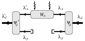
Figure 13: The deuteron tensor in tagged DIS in the IA. Only the spin quantum numbers of the deuteron and nucleon states are shown.

The summation over the nucleon LF helicities in Eq. (264) and deuteron spin in Eq. (263) can be performed using the neutron spin density matrix formalism described in Sec. V.1. The neutron tensor is represented as a bilinear form in LF bispinors,

$$W_{n}^{\mu\nu}(p_{n},\widetilde{q};{\lambda^{\prime}}_{\!\!n},\lambda_{n})\; =\;\bar{u}_{\rm LF}(p_{n},{\lambda^{\prime}}_{\!\!n})\;\Gamma_{n}^{\mu\nu}(p_{n},\widetilde{q})\;$$

$$\times u_{\rm LF}(p_{n},\lambda_{n}),$$ (267)

where $\Gamma_{n}^{\mu\nu}$ is matrix in bispinor indices, whose specific form is given below. The deuteron tensor of the ensemble, Eq. (263), can then be expressed as a bispinor trace,

$$W_{d}^{\mu\nu}(p_{d},q,p_{p})\; =\;[2(2\pi)^{3}]\;\frac{2}{(2-\alpha_{p})^{2}}$$

$$\times\;\textrm{tr}[\,\Pi_{n}(p_{d},p_{p};s_{n})\;\Gamma_{n}^{\mu\nu}(p_{n},\widetilde{q})\,],$$ (268)

where $\Pi_{n}$ is the effective neutron spin density matrix Eq. (193b). [In contrast to Eq. (193a), there is no integration over the proton LF momentum variables $\alpha_{p}$ and $\alpha_{p}$, as those are fixed to the tagged proton values.] Equation (267) represents the IA result for a general deuteron ensemble.

To determine the tagged DIS structure functions, one evaluates the tensor equation Eq. (268) with the specific form of the neutron tensor (unpolarized, polarized) and the neutron spin density matrix (unpolarized, vector, tensor), and derives equations for the structure functions by taking suitable components of the tensor equation. To separate the various structure functions one needs to use both $+$ and $T$ LF components of the deuteron and nucleon tensors. It is known that in LF quantization of interacting spin-1/2 systems the $+$ and $T$ components of the current operator have different status: the $+$ current components are formed from the independent canonical degrees of freedom and are free of interactions (“good components”); the $T$ components involve dependent degrees of freedom and thus depend on the interactions (“bad components”). The use of bad components in the IA therefore generally must be regarded as an approximation. However, studies have shown that the interaction effects in the $T$ components of the current are suppressed in the DIS limit $Q^{2}\gg m^{2},x$ fixed, i.e., that they do not affect the result for the leading structure functions in the DIS limit (leading-twist approximation) Frankfurt and Strikman (1988); Lev et al. (1998). In the following calculations we consider only the leading structure functions in the DIS limit (unpolarized, polarized), for which the use of $T$ components is justified. This is supported by the fact that the IA structure functions in the DIS limit satisfy the sum rules for baryon number, LF momentum, and spin (see below).

We note that the calculations could in principle be extended to power-suppressed structures in the DIS limit, such as the spin structure functions $F_{[LS_{T}]d}$ or $g_{2d}$ (see Sec. III.7). In this case the interaction effects in the $T$ components of the current could no longer be neglected, and new considerations would be needed — the so-called angular conditions on the current matrix elements Frankfurt and Strikman (1988); Lev et al. (1998).

VI.2 Unpolarized electron scattering

Unpolarized electron scattering involves the symmetric parts of the deuteron and neutron tensors. The symmetric part of the neutron tensor is diagonal in the neutron LF helicities and independent of the value of the helicity,

$$W^{\mu\nu}_{n}(p_{n},\widetilde{q};{\lambda^{\prime}}_{\!\!n},\lambda_{n})[\textrm{symm}]$$

$$=\;\delta({\lambda^{\prime}}_{\!\!n},\lambda_{n})\;W^{\mu\nu}_{n}(p_{n},\widetilde{q})[\textrm{symm}].$$ (269)

In the bilinear form Eq. (267) the tensor is therefore represented by the unit matrix in bispinor indices

$$\Gamma^{\mu\nu}_{n}\;\;=\;\;\frac{1}{2m}\;W^{\mu\nu}_{n}[\textrm{symm}].$$ (270)

The unpolarized symmetric deuteron tensor is then obtained from Eq. (268) as

$$W^{\mu\nu}_{d}[\textrm{unpol}]\,=\,[2(2\pi)^{3}]\;\frac{2\mathcal{S}_{d}[\textrm{unpol}]}{2-\alpha_{p}}\,W^{\mu\nu}_{n}[\textrm{symm}].$$ (271)

The relation between the tensors is, up to a factor, given by the helicity-independent neutron distribution in the unpolarized deuteron, Eq. (225b).

The decomposition of the symmetric neutron tensor is of the same form as that of the unpolarized deuteron tensor Eq. (44),

$$W_{n}^{\mu\nu}[\textrm{symm}]\; =\;\frac{1}{2}(e_{L}^{\mu}e_{L}^{\nu}-e_{q}^{\mu}e_{q}^{\nu}-g^{\mu\nu})\,F_{[UU,T]n}$$ (272)

$$+\;\frac{1}{2}e_{L}^{\mu}e_{L}^{\nu}\,F_{[UU,L]n},$$

where now the basis vectors $e_{L}$ and $e_{q}$ are constructed with the 4-momenta $p_{n}$ and $\widetilde{q}$, and the structure functions depend on invariants formed with the latter. Substituting this form in Eq. (271), taking suitable components of the tensor equation ($\mu\nu=++$ and $TT$), one obtains expressions for the tagged deuteron structure functions Strikman and Weiss (2018)

$$F_{[UU,T]d}(x,Q^{2};\alpha_{p},\bm{p}_{pT})$$

$$=\;[2(2\pi)^{3}]\;\frac{2\mathcal{S}_{d}(\alpha_{p},\bm{p}_{pT})[\textrm{unpol}]}{2-\alpha_{p}}\;F_{[UU,T]n}(\widetilde{x},Q^{2}),$$ (273a)

$$F_{[UU,L]d}(x,Q^{2};\alpha_{p},\bm{p}_{pT})$$

$$=\;[2(2\pi)^{3}]\;\frac{2\mathcal{S}_{d}(\alpha_{p},\bm{p}_{pT})[\textrm{unpol}]}{2-\alpha_{p}}\;F_{[UU,L]n}(\widetilde{x},Q^{2}),$$ (273b)

$$\widetilde{x}\;\equiv\;\frac{x}{2-\alpha_{p}}.$$ (273c)

$\tilde{x}$ is the effective scaling variable for scattering on the neutron, which takes into account its longitudinal LF momentum in the deuteron. The expressions Eqs. (273a)–(273c) are valid in the DIS limit $Q^{2}\gg m^{2}$, neglecting kinematic corrections ${\mathcal{O}}(m^{2}/Q^{2})$. The corresponding expressions for the tagged deuteron structure functions $F_{1d}$ and $F_{2d}$, Eq. (53), are

$$F_{1d}(x,Q^{2};\alpha_{p},\bm{p}_{pT})$$

$$=\;[2(2\pi)^{3}]\;\frac{2\mathcal{S}_{d}(\alpha_{p},\bm{p}_{pT})[\textrm{unpol}]}{2-\alpha_{p}}\;F_{1n}(\widetilde{x},Q^{2}),$$ (274a)

$$F_{2d}(x,Q^{2};\alpha_{p},\bm{p}_{pT})$$

$$=\;[2(2\pi)^{3}]\;\;\mathcal{S}_{d}(\alpha_{p},\bm{p}_{pT})[\textrm{unpol}]\;F_{2n}(\widetilde{x},Q^{2}).$$ (274b)

The tagged deuteron $F_{2d}$ and the neutron $F_{2n}$ are related directly by the neutron momentum distribution in the deuteron.

The neutron momentum distribution satisfies the LF momentum sum rule Eq. (229a). It implies that the integrated tagged structure function [see Eq. (152); note the kinematic limit $\alpha_{p}<2-x$]

$$F_{2d}^{\rm int}(x,Q^{2})\; \equiv\;[2(2\pi)^{3}]^{-1}\int_{0}^{2-x}\frac{d\alpha_{p}}{\alpha_{p}}\int d^{2}p_{pT}$$

$$\times\;F_{2d}(x,Q^{2};\alpha_{p},p_{pT})$$ (275)

satisfies the sum rule

$$\int_{0}^{2}dx\;F_{2d}^{\rm int}(x,Q^{2})\;\;=\;\;\int_{0}^{1}d\widetilde{x}\;F_{2n}(\widetilde{x},Q^{2}).$$ (276)

It shows that spectator tagging only fixes the neutron LF momentum in the deuteron but does not change the integral of the distribution.

The tensor-polarized part of the symmetric deuteron tensor is obtained from Eq. (268) as

$$W^{\mu\nu}_{d}[\textrm{tensor}]\; =\;[2(2\pi)^{3}]\;\frac{2\mathcal{S}_{d}[\textrm{tensor}]}{2-\alpha_{p}}$$

$$\times\;W^{\mu\nu}_{n}[\textrm{symm}],$$ (277)

where the tensor-polarized neutron distribution is given in Eq. (225c), and the symmetric neutron tensor is the same as above. Equation (277) holds for an ensemble with general tensor polarization. The calculation of the tensor-polarized structure functions proceeds in the same way as for the unpolarized deuteron. Here we quote only the expressions for the tensor structure functions $F_{[UT_{LL},T]d}$ and $F_{[UT_{LL},L]d}$, which appear in the calculation of spin asymmetries in the scaling limit (see Sec. III.7 and below). They can be obtained with the special polarization tensor associated with pure states, Eq. (218e), choosing the polarization along the $z$-direction, $\bm{N}=\bm{e}_{z}$. We obtain

$$T_{LL}F_{[UT_{LL},T]d}(x,Q^{2};\alpha_{p},\bm{p}_{pT})$$

$$=\;[2(2\pi)^{3}]\;\frac{2\mathcal{S}_{d}(\alpha_{p},\bm{p}_{pT})[\textrm{tensor}]}{2-\alpha_{p}}\;F_{[UU,T]n}(\widetilde{x},Q^{2}),$$ (278a)

$$T_{LL}F_{[UT_{LL},L]d}(x,Q^{2};\alpha_{p},\bm{p}_{pT})$$

$$=\;[2(2\pi)^{3}]\;\frac{2\mathcal{S}_{d}(\alpha_{p},\bm{p}_{pT})[\textrm{tensor}]}{2-\alpha_{p}}\;F_{[UU,L]n}(\widetilde{x},Q^{2}),$$ (278b)

where $\mathcal{S}_{d}(\alpha_{p},\bm{p}_{pT})[\textrm{tensor}]$ is the neutron distribution given in Eq. (251a).

VI.3 Polarized electron scattering

Polarized electron scattering involves the antisymmetric parts of the deuteron and neutron tensors. The antisymmetric part of the neutron tensor depends on the neutron LF helicities. This dependence can be expressed in the form

$$W^{\mu\nu}_{n}(p_{n},\widetilde{q};{\lambda^{\prime}}_{\!\!n},\lambda_{n})[\textrm{antisymm}]$$

$$=\;A^{\mu\nu}_{\phantom{\mu\nu}\rho}(p_{n},\widetilde{q})\;s_{n,\textrm{gen}}^{\rho}(p_{n},{\lambda^{\prime}}_{\!\!n},\lambda_{n}),$$ (279a)

$$s_{n,\textrm{gen}}^{\rho}(p_{n},{\lambda^{\prime}}_{\!\!n},\lambda_{n})$$

$$\equiv\;\frac{1}{2m}\,\bar{u}_{\rm LF}(p_{n},{\lambda^{\prime}}_{\!\!n})\,(-\gamma^{\rho}\gamma^{5})\,u_{\rm LF}(p_{n},\lambda_{n}).$$ (279b)

The axial 4-vector $s_{n,\textrm{gen}}$ is defined as a function of the LF helicities, $\lambda_{n}$ and ${\lambda^{\prime}}_{\!\!n}$, and represents the general polarization 4-vector of the free neutron. The tensor $A^{\mu\nu}_{\phantom{\mu\nu}\rho}$ is given by [cf. Eq. (62)]

$$A^{\mu\nu}_{\phantom{\mu\nu}\rho}\; =\;\frac{i}{2}\epsilon^{\mu\nu\sigma\tau}e_{q,\sigma}\left\{e_{L\ast\tau}e_{L\ast\rho}\,\gamma F_{[LS_{L}]n}\right.$$

$$+\;\left.\left(e_{L\ast\tau}e_{L\ast\rho}+g_{\tau\rho}\right)F_{[LS_{T}]n}\right\}$$

where the basis vectors $e_{L\ast}$ and $e_{q}$ are constructed with the 4-momenta $p_{n}$ and $\widetilde{q}$, and the structure functions depend on invariants formed with the latter. In the bilinear form Eq. (267) the antisymmetric neutron tensor is therefore represented by the matrix

$$\Gamma^{\mu\nu}_{n}\; = \;\frac{1}{2m}\,A^{\mu\nu}_{\phantom{\mu\nu}\rho}\;(-\gamma^{\rho}\gamma^{5}).$$ (280)

The trace in Eq. (268) now involves the vector-polarized part of the neutron density matrix, Eq. (202),

$$\textrm{tr}\left[\Pi_{n}\Gamma_{n}^{\mu\nu}\right]\; =\;\frac{1}{2m}\,A^{\mu\nu}_{\phantom{\mu\nu}\rho}\,\textrm{tr}[{\textstyle\frac{1}{2}}(p_{n}\gamma+m)(s_{n}\gamma)\gamma^{5}\;(-\gamma^{\rho}\gamma^{5})]$$

$$=\;A^{\mu\nu}_{\phantom{\mu\nu}\rho}\;s_{n}^{\rho},$$ (281a)

where $s_{n}$ is now the effective neutron polarization vector in the deuteron, Eq. (202b). Altogether, the vector-polarized deuteron tensor is obtained from Eq. (268) as

$$W^{\mu\nu}_{d}(p_{d},q,p_{p})[\textrm{vector}]\; =\;[2(2\pi)^{3}]\;\frac{2}{(2-\alpha_{p})^{2}}\;A^{\mu\nu}_{\phantom{\mu\nu}\rho}\;s_{n}^{\rho}.$$ (282)

In the last expressions

$$A^{\mu\nu}_{\phantom{\mu\nu}\rho}\;s_{n}^{\rho}\;\;\equiv\;\;W^{\mu\nu}_{n}(p_{n},\widetilde{q},s_{n})[\textrm{antisymm}]$$ (283)

is the antisymmetric neutron tensor, evaluated with the effective polarization 4-vector $s_{n}$, Eq. (202b). All the information pertaining to the deuteron wave function (radial functions, polarization, etc.) is contained in $s_{n}$. The entire effect of averaging with the effective neutron density matrix has been to replace the general neutron polarization 4-vector of the free neutron in Eq. (279a) with the specific polarization 4-vector of the neutron in the deuteron of Eq. (202b). This simple result is achieved thanks to the covariant representation of the deuteron spin structure cf. Secs. IV and V.

We can now derive the expression for the tagged deuteron spin structure functions. As before we consider the DIS limit, in which the structure function $F_{[LS_{L}]d}$ is leading and $F_{[LS_{T}]d}$ is suppressed, and neglect terms ${\mathcal{O}}(m/Q)$. The derivation proceeds as follows: (a) Take the tensor equation Eq. (282) in a general collinear frame with $p_{d}^{+}\neq M_{d}$; (b) take the deuteron longitudinally polarized, corresponding to a rest-frame polarization vector $\bm{S}=(\bm{0}_{T},S^{z})$, cf. Eq. (201). (c) take the non-zero transverse component of the tensor equation, $\mu\nu=12$. In this way we obtain, after a brief calculation,

$$F_{[LS_{L}]d}(x,Q^{2};\alpha_{p},\bm{p}_{pT})$$

$$=\;[2(2\pi)^{3}]\;\frac{4ms_{n}^{+}}{(2-\alpha_{p})^{3}\,p_{d}^{+}\,S^{z}}\;F_{[LS_{L}]n}(\widetilde{x},Q^{2}).$$ (284)

$\widetilde{x}$ is defined in Eq. (273c). The ratio on the R.H.S. is, up to a factor, equal to the helicity-dependent LF momentum distribution of neutrons in the deuteron state with LF helicity $+1$, Eq. (253), and we can write

$$F_{[LS_{L}]d}(x,Q^{2};\alpha_{p},\bm{p}_{pT})$$

$$=\;[2(2\pi)^{3}]\;\frac{2\Delta\mathcal{S}_{d}(\alpha_{p},\bm{p}_{pT})[\textrm{pure $+1$}]}{2-\alpha_{p}}\;F_{[LS_{L}]n}(\widetilde{x},Q^{2}).$$ (285)

The corresponding expression for the tagged spin structure function $g_{1d}$ is

$$g_{1d}(x,Q^{2};\alpha_{p},\bm{p}_{pT})$$

$$=\;[2(2\pi)^{3}]\;\frac{2\Delta\mathcal{S}_{d}(\alpha_{p},\bm{p}_{pT})[\textrm{pure $+1$}]}{2-\alpha_{p}}\;g_{1n}(\widetilde{x},Q^{2}).$$ (286)

The formula applies in the DIS limit, where $\gamma\rightarrow 0$ and the contribution of the $g_{2}$ structure function is suppressed; the formulas including power corrections can be derived easily.

The helicity-dependent neutron distribution in the deuteron satisfies the spin sum rule Eq. (233). It implies that the integrated tagged spin structure function

$$g_{1d}^{\rm int}(x,Q^{2})\; \equiv\;[2(2\pi)^{3}]^{-1}\int_{0}^{2-x}\frac{d\alpha_{p}}{\alpha_{p}}\int d^{2}p_{pT}$$

$$\times\;g_{1d}(x,Q^{2};\alpha_{p},p_{pT})$$ (287)

satisfies the sum rule

$$\int_{0}^{2}dx\;g_{1d}^{\rm int}(x,Q^{2})\; =\;\frac{g_{Ad}}{g_{A}}\;\int_{0}^{1}d\widetilde{x}\;g_{1n}(\widetilde{x},Q^{2})$$ (288a)

$$=\;2\left(1-\frac{3}{2}\omega_{2}\right)\;\int_{0}^{1}d\widetilde{x}\;g_{1n}(\widetilde{x},Q^{2}).$$ (288b)

Eq. (288a) is obtained by changing the order of integrations over $x$ and $\alpha_{p}$ and substituting $x$ by $\widetilde{x}$, Eq. (273c). The last expression applies when the axial charge is evaluated in the non-relativistic limit, Eq. (244). We see that our result for the integrated tagged spin structure function reproduces the nonrelativistic formula for the D-state correction to the deuteron spin structure function.

VI.4 Spin asymmetries

Using the results for the tagged spin structure functions in the IA, we now calculate the spin asymmetries in tagged DIS. In the DIS limit $\gamma\rightarrow 0$ only the parallel spin asymmetries $A_{\parallel}$ are present. The scaling variable $y$ and the virtual photon polarization parameter $\epsilon$, and therefore the depolarization factors $D_{\parallel[S_{L}]}$, are the same for DIS on the deuteron and the (bound) neutron up to power corrections,

$$\epsilon[\textrm{deuteron}]\; =\;\epsilon[\textrm{neutron}]\;+\;{\mathcal{O}}(m^{2}/Q^{2}),$$ (289a)

$$D_{\parallel[S_{L}]}[\textrm{deuteron}]\; =\;D_{\parallel[S_{L}]}[\textrm{neutron}]\;+\;{\mathcal{O}}(m^{2}/Q^{2});$$ (289b)

we do not distinguish between the deuteron and neutron in the notation of these quantities. Following Sec. III.7 we consider both the three-state and the two-state asymmetries, Eqs. (107) and (109). Substituting the expressions for the tagged structure functions in the IA, the deuteron three-state asymmetry Eq. (107) becomes

$$A_{\parallel(3)d}(x,Q^{2};\alpha_{p},\bm{p}_{pT})$$

$$=\;\frac{D_{\parallel[S_{L}]}\;F_{[LS_{L}]d}(x,Q^{2};\alpha_{p},\bm{p}_{pT})}{[F_{[UU,T]d}\;+\;\epsilon F_{[UU,L]d}](x,Q^{2};\alpha_{p},\bm{p}_{pT})}$$ (290a)

$$=\;\frac{\Delta\mathcal{S}_{d}(\alpha_{p},\bm{p}_{pT})[\textrm{pure $+1$}]\;D_{\parallel[S_{L}]}\;F_{[LS_{L}]n}(\widetilde{x},Q^{2})}{\mathcal{S}_{d}(\alpha_{p},\bm{p}_{pT})[\textrm{unpol}]\;[F_{[UU,T]n}\;+\;\epsilon F_{[UU,L]n}](\widetilde{x},Q^{2})}$$ (290b)

$$=\;\mathcal{D}_{\parallel(3)d}(\alpha_{p},\bm{p}_{pT})\;A_{\parallel n}(y,\widetilde{x},Q^{2}),$$ (290c)

$$\mathcal{D}_{\parallel(3)d}(\alpha_{p},\bm{p}_{pT})\; \equiv\;\frac{\Delta\mathcal{S}_{d}(\alpha_{p},\bm{p}_{pT})[\textrm{pure $+1$}]}{\mathcal{S}_{d}(\alpha_{p},\bm{p}_{pT})[\textrm{unpol}]},$$ (290d)

$$A_{\parallel n}(y,\widetilde{x},Q^{2})\; \equiv\;\frac{D_{\parallel[S_{L}]}\;F_{[LS_{L}]n}(\widetilde{x},Q^{2})}{[F_{[UU,T]n}\;+\;\epsilon F_{[UU,L]n}](\widetilde{x},Q^{2})}.$$ (290e)

The tagged deuteron asymmetry can be factorized into the neutron spin asymmetry and a function describing deuteron structure. $A_{\parallel n}$ is the ratio of the polarized and unpolarized neutron structure functions and the depolarization factor; it represents the parallel spin asymmetry for scattering on the neutron and depends on the nucleon subprocess variables, $\widetilde{x}$ and $Q^{2}$, as well as on $y$. $\mathcal{D}_{\parallel(3)d}$ is the ratio of helicity-dependent and -independent neutron distributions in the deuteron and depends on the proton momentum variables $\alpha_{p}$ and $\bm{p}_{pT}$. We refer to this function as the deuteron depolarization factor. Note that the unpolarized neutron distribution in Eq. (290d) represents the average of the three pure deuteron states with LF helicities $\pm 1$ and $0$, so that

$$\mathcal{D}_{\parallel(3)d} =\frac{\Delta\mathcal{S}_{d}[\textrm{pure $+1$}]}{\frac{1}{3}\left(\mathcal{S}_{d}[\textrm{pure $+1$}]+\mathcal{S}_{d}[\textrm{pure $-1$}]+\mathcal{S}_{d}[\textrm{pure $0$}]\right)}.$$ (291)

Its explicit form as a function of the CM momentum variable is

$$\mathcal{D}_{\parallel(3)d}= \frac{\displaystyle\left(f_{0}-\frac{f_{2}}{\sqrt{2}}\right)\left(C_{0}f_{0}-\frac{C_{2}f_{2}}{\sqrt{2}}\right)}{f_{0}^{2}+f_{2}^{2}}$$

$$[f_{0,2}\equiv f_{0,2}(k);\,C_{0,2}\equiv C_{0,2}(\bm{k})].$$ (292)

The two-state asymmetry Eq. (109) in the DIS limit is given by

$$A_{\parallel(2)d}(x,Q^{2};\alpha_{p},\bm{p}_{pT})\; =\;\frac{D_{\parallel[S_{L}]}\;F_{[LS_{L}]}(x,Q^{2};\alpha_{p},\bm{p}_{pT})}{\left[F_{[UU,T]d}\;+\;\epsilon F_{[UU,L]d}\;+\;D_{\parallel[T_{LL}]}\,(F_{[UT_{LL},T]d}+\epsilon F_{[UT_{LL},L]d})\right](x,Q^{2};\alpha_{p},\bm{p}_{pT})}.$$ (293)

Now, in addition to the unpolarized structure functions, the tensor-polarized structure functions $F_{[UT_{LL},T]d}$ and $F_{[UT_{LL},L]d}$ appear in denominator. In the IA they are given by Eqs. (278a) and (278b) in terms of the neutron distribution in the tensor-polarized deuteron and the unpolarized neutron structure functions. In Eq. (293) $D_{\parallel[T_{LL}]}$ is the depolarization factor given by Eq. (99a). In the DIS limit it becomes

$$D_{\parallel[T_{LL}]}\;=\;\frac{1}{3}\;+\;{\mathcal{O}}(m^{2}/Q^{2}).$$ (294)

Substituting the expressions for the tagged structure functions in the IA, the asymmetry can be factorized in a similar way as Eq. (290c),

$$A_{\parallel(2)d}(x,Q^{2};\alpha_{p},\bm{p}_{pT})$$

$$=\mathcal{D}_{\parallel(2)d}(\alpha_{p},\bm{p}_{pT})\;A_{\parallel n}(\widetilde{x},Q^{2}),$$ (295a)

$$\mathcal{D}_{\parallel(2)d}(\alpha_{p},\bm{p}_{pT})$$

$$\equiv\frac{\Delta\mathcal{S}_{d}(\alpha_{p},\bm{p}_{pT})[\textrm{pure $+1$}]}{\mathcal{S}_{d}(\alpha_{p},\bm{p}_{pT})[\textrm{unpol}]+\mathcal{S}_{d}(\alpha_{p},\bm{p}_{pT})[\textrm{tensor}]}.$$ (295b)

The deuteron depolarization factor now includes the tensor-polarized neutron distribution in the denominator. Note that the sum of unpolarized and tensor neutron distributions in Eq. (295b) represents the sum of the two pure deuteron states with LF helicities $\pm 1$, so that

$$\mathcal{D}_{\parallel(2)d} =\frac{\Delta\mathcal{S}_{d}[\textrm{pure $+1$}]}{\frac{1}{2}\left(\mathcal{S}_{d}[\textrm{pure $+1$}]+\mathcal{S}_{d}[\textrm{pure $-1$}]\right)}.$$ (296)

This function is related to the effective neutron polarization in the pure $+1$ state, Eq. (259), and is bounded as

$$-1\;\leq\;\mathcal{D}_{\parallel(2)d}\;\leq\;1.$$ (297)

Its explicit form as a function of the CM momentum variable is

$$\mathcal{D}_{\parallel(2)d}= \frac{\displaystyle\left(f_{0}-\frac{f_{2}}{\sqrt{2}}\right)\left(C_{0}f_{0}-\frac{C_{2}f_{2}}{\sqrt{2}}\right)}{\displaystyle f_{0}^{2}+f_{2}^{2}-C_{T}\left(2f_{0}+\frac{f_{2}}{\sqrt{2}}\right)\frac{f_{2}}{\sqrt{2}}}$$ (298)

$$[f_{0,2}\equiv f_{0,2}(k),\,C_{0,2,T}\equiv C_{0,2,T}(\bm{k})].$$

Figure 14: The deuteron depolarization factors $\mathcal{D}_{\parallel(3)d}$ (three-state asymmetry) and $\mathcal{D}_{\parallel(2)d}$ (two-state asymmetry) in polarized tagged DIS. The graph shows the depolarization factors at $\alpha_{p}=1$ as functions of $|\bm{p}_{pT}|$.

The deuteron depolarization factors $\mathcal{D}_{\parallel(3)d}$ and $\mathcal{D}_{\parallel(2)d}$ describe the effective neutron polarization “selected” by the tagged proton momentum and summarize the deuteron structure effects in spin asymmetry measurements in tagged DIS. Figure 14 shows $\mathcal{D}_{\parallel(3)d}$ and $\mathcal{D}_{\parallel(2)d}$ at $\alpha_{p}=1$ as functions of $|\bm{p}_{pT}|$. One observes: (a) Both $\mathcal{D}_{\parallel(3)d}$ and $\mathcal{D}_{\parallel(2)d}$ are unity at $\alpha_{p}=1$ and $|\bm{p}_{pT}|=0$, where $|\bm{k}|=0$ and only the S-wave is present. (b) $\mathcal{D}_{\parallel(3)d}$ and $\mathcal{D}_{\parallel(2)d}$ remain close to unity for $|\bm{p}_{pT}|\lesssim$ 150 MeV, where the S-wave dominates. The D-wave contributions raise $\mathcal{D}_{\parallel(3)d}$ above unity but lower $\mathcal{D}_{\parallel(2)d}$, in accordance with the bound Eq. (297), showing the effect of the tensor polarized structure in $\mathcal{D}_{\parallel(2)d}$. (c) Both $\mathcal{D}_{\parallel(3)d}$ and $\mathcal{D}_{\parallel(2)d}$ decrease significantly at $|\bm{p}_{pT}|\gtrsim$ 150 MeV, pass through zero at $|\bm{p}_{pT}|\approx$ 300 MeV, where the combination $(f_{0}-f_{2}/\sqrt{2})$ vanishes, and become negative at larger momenta, where the D-wave dominates.

Figure 15: The deuteron depolarization factors $\mathcal{D}_{\parallel(3)d}$ (three-state asymmetry, upper graph) and $\mathcal{D}_{\parallel(2)d}$ (two-state asymmetry, lower graph), as functions of $|\bm{p}_{pT}|$, for several values of $\alpha_{p}$. Note the different scales on the vertical axis in the upper and lower plots.

Important differences between the three-state and two-state depolarization factors appear in the behavior at small proton momenta. Because the factors $C_{0},C_{2}$ and $C_{T}$ become unity at $\bm{k}_{T}=0$,

$$\mathcal{D}_{\parallel(2)d}\; = \;1\hskip 10.00002pt\textrm{at}\hskip 10.00002pt\textrm{$|\bm{p}_{pT}|=0$, \, $\alpha_{p}$ arbitrary.}$$ (299)

In contrast, $\mathcal{D}_{\parallel(3)d}\neq 1$ for $|\bm{p}|_{pT}=0$ and $\alpha_{p}$ arbitrary; the value at $|\bm{p}_{pT}|=0$ is unity only if $\alpha_{p}=1$. Figure 15 shows $\mathcal{D}_{\parallel(2)d}$ and $\mathcal{D}_{\parallel(3)d}$ as functions of $|\bm{p}_{pT}|$ for several values of $\alpha_{p}$. One observes that at small proton momenta the values of $\mathcal{D}_{\parallel(2)d}$ are much closer to unity than those of $\mathcal{D}_{\parallel(3)d}$. This difference can also be seen in the expressions Eqs. (292) and (298), when one substitutes the factors $C_{0},C_{2}$ and $C_{T}$ by their approximate forms for small CM momenta $\bm{k}\ll m$,

$$C_{0}\; =\;1\;+\;{\mathcal{O}}(\bm{k}/m),$$ (300a)

$$C_{2}\; =\;1-\frac{3|\bm{k}_{T}|^{2}}{|\bm{k}|^{2}}\;+\;{\mathcal{O}}(\bm{k}/m),$$ (300b)

$$C_{T}\; =\;1-\frac{3|\bm{k}_{T}|^{2}}{2|\bm{k}|^{2}}\;+\;{\mathcal{O}}(\bm{k}/m).$$ (300c)

In this approximation

$$\left(f_{0}-\frac{f_{2}}{\sqrt{2}}\right)\left(C_{0}f_{0}-\frac{C_{2}f_{2}}{\sqrt{2}}\right)$$

$$=\;f_{0}^{2}-\left(2-\frac{3|\bm{k}_{T}|^{2}}{|\bm{k}|^{2}}\right)\frac{f_{0}f_{2}}{\sqrt{2}}+\left(1-\frac{3|\bm{k}_{T}|^{2}}{|\bm{k}|^{2}}\right)\frac{f_{2}^{2}}{2},$$ (301a)

$$f_{0}^{2}+f_{2}^{2}-C_{T}\left(2f_{0}+\frac{f_{2}}{\sqrt{2}}\right)\frac{f_{2}}{\sqrt{2}}$$

$$=\;f_{0}^{2}-\left(2-\frac{3|\bm{k}_{T}|^{2}}{|\bm{k}|^{2}}\right)\frac{f_{0}f_{2}}{\sqrt{2}}+\left(1+\frac{3|\bm{k}_{T}|^{2}}{2|\bm{k}|^{2}}\right)\frac{f_{2}^{2}}{2}.$$ (301b)

One sees that in $\mathcal{D}_{\parallel(2)d}$ the numerator and denominator coincide in terms linear in the D-wave and differ only in terms quadratic in the D-wave; in $\mathcal{D}_{\parallel(3)d}$ the numerator and denominator differ already in terms linear in the D-wave. Consequently,

$$\left.\begin{array}[]{lcl}\mathcal{D}_{\parallel(2)d}&=&\;1\;+\;\textrm{terms}\;f_{2}^{2}/f_{0}^{2}\\[4.30554pt] \mathcal{D}_{\parallel(3)d}&=&\;1\;+\;\textrm{terms}\;f_{2}/f_{0}\end{array}\right\}\hskip 10.00002pt(|\bm{k}|\ll m).$$ (304)

D-wave corrections affect $\mathcal{D}_{\parallel(2)d}$ at only quadratic order at low momenta, but $\mathcal{D}_{\parallel(3)d}$ already at linear order.

The deviation of $\mathcal{D}_{\parallel(2)d}$ from unity can be computed using a simple approximate formula. At CM momenta $k\lesssim 0.1$ GeV the ratio of D- and S-wave functions is approximately given by

$$\frac{f_{2}(k)}{f_{0}(k)}\;\approx\;\frac{k^{2}}{\lambda^{2}},$$ (305)

where $\lambda^{2}\approx 0.087$ GeV² for the AV18 wave functions Wiringa et al. (1995). Expanding the ratio of Eqs. (301a) and (301b) to first order in $f_{2}^{2}/f_{0}^{2}$, we then obtain

$$\mathcal{D}_{\parallel(2)d}\; \approx\;1-\frac{9|\bm{k}_{T}|^{2}}{4|\bm{k}|^{2}}\left[\frac{f_{2}(k)}{f_{0}(k)}\right]^{2}$$

$$\approx\;1-\frac{9\,|\bm{k}_{T}|^{2}\,|\bm{k}|^{2}}{4(\lambda^{2})^{2}}.$$ (306)

The expression of the CM momentum variable in terms of the original LF variables $\alpha_{p}$ and $\bm{p}_{pT}$ is given in Eq. (177).

VII Neutron spin structure extraction

VII.1 Analytic properties of light-front wave function

We are now ready to study the extraction of neutron structure functions from tagged deuteron DIS measurements. In general, for arbitrary nonzero values of the proton momentum, the tagged cross section is modified by initial-state nuclear binding effects beyond those included in the $pn$ LF wave function (non-nucleonic degrees of freedom, modified nucleon structure), and by final-state interactions beyond the IA (scattering of slow hadrons in the DIS final state from the spectator nucleon). These effects can be eliminated by pole extrapolation in the proton momentum Sargsian and Strikman (2006); Strikman and Weiss (2018). The method uses the analytic properties of the deuteron wave function to select $pn$ configurations in the deuteron with infinite transverse separation, in which both nuclear binding effects and final-state interactions are suppressed. It permits model-independent extraction of free neutron structure. Here we review its use in the unpolarized case, and then apply it to the polarized case.

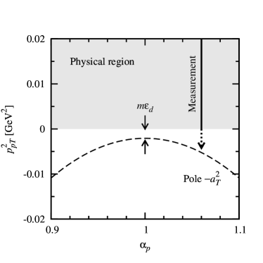
Figure 16: The kinematic variables $\alpha_{p}$ and $p_{pT}^{2}\equiv|\bm{p}_{pT}|^{2}$ in neutron structure measurements with pole extrapolation. The physical region $p_{pT}^{2}>0$ is shown by the shaded area. The pole position at $p_{pT}^{2}=-a_{T}^{2}$ is shown by the dashed line. The tagged structure functions are measured at fixed $\alpha_{p}$ as functions of $p_{pT}^{2}$ in the physical region as indicated by the solid line. The measurements are then extrapolated to the pole as indicated by the dotted line.

To discuss the analytic properties in the proton transverse momentum, we regard the deuteron wave function as a function of the invariant mass of the $pn$ pair, Eq. (161b)

$$M_{pn}^{2}\; =\;\frac{4(|\bm{p}_{pT}|^{2}+m^{2})}{\alpha_{p}(2-\alpha_{p})},$$ (307)

which takes values $M_{pn}^{2}\geq 4m^{2}$ for physical proton momenta. In this variable the wave function has a pole singularity of the form (we suppress the spin structure for the moment)

$$\Psi_{d}(\alpha_{p},\bm{p}_{pT})\; =\;\frac{\textrm{Residue}}{M_{pn}^{2}-M_{d}^{2}}\;+\;\textrm{(less singular)},$$ (308)

which follows from the general properties of the LF bound-state equation. It lies outside the physical region of proton momenta because $M_{pn}^{2}\geq 4m^{2}>M_{d}^{2}$. The pole in the invariant mass implies a pole in the transverse momentum of the form

$$\Psi_{d}(\alpha_{p},\bm{p}_{pT})\; =\;\frac{\textrm{Residue}}{|\bm{p}_{pT}|^{2}+a_{T}^{2}}\;+\;\textrm{(less singular)},$$ (309)

$$a_{T}^{2}\; =\;a_{T}^{2}(\alpha_{p})\;\equiv\;m^{2}-\alpha_{p}(2-\alpha_{p})\frac{M_{d}^{2}}{4}.$$ (310)

It lies in the unphysical region $|\bm{p}_{pT}|^{2}<0$ (see Fig. 16). The pole position $a_{T}^{2}$ depends on $\alpha_{p}$. The minimum value of $a_{T}^{2}$ occurs at $\alpha_{p}=1$ and is

$$a_{T}^{2}[\textrm{min}]=m^{2}-\frac{M_{d}^{2}}{4}=m\epsilon_{d}+\mathcal{O}(\epsilon_{d}^{2})=a^{2},$$ (311)

where $\epsilon_{d}\equiv 2m-M_{d}$ is the deuteron binding energy and $a^{2}\equiv m\epsilon_{d}$ is the inverse squared Bethe-Peierls radius of the deuteron.

The singularity in the transverse momentum Eq. (309) has a simple physical interpretation. It is related to the asymptotic behavior of the transverse coordinate-space wave function at large transverse separations of the $pn$ pair. When the transverse momentum-space wave function is represented as a Fourier transform of the transverse-coordinate wave function, the singularity arises from the contribution of large transverse separations $r_{T}\rightarrow\infty$ to the Fourier integral. In this sense the singularity describes the presence of $pn$ configurations with large (infinite) transverse separation in the deuteron wave function at unphysical momenta. (The interpretation of the pole in the invariant formulation in terms of Feynman diagrams is discussed below.)

In the representation of the deuteron LF wave function in terms of the CM momentum, the invariant mass of the $pn$ configuration is

$$M_{pn}^{2}\; =\;4(|\bm{k}|^{2}+m^{2}).$$ (312)

The pole Eq. (308) appears through the pole of the S-wave radial function

$$f_{0}(k)\; =\;\frac{\sqrt{m}\,\Gamma}{|\bm{k}|^{2}+a^{2}}\;+\;\textrm{(less singular)},$$ (313)

which is obtained from the 3-dimensional bound state equation and represents a general feature of the weakly bound system. The residue $\Gamma$ can be inferred from the non-relativistic approximation (see Sec. IV.4). This again shows the close correspondence between the LF and the nonrelativistic description of the two-body bound state.

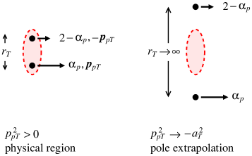
Figure 17: Coordinate-space interpretation of the pole extrapolation. Left: Physical transverse momenta $p_{pT}^{2}>0$ correspond to $pn$ configurations of finite transverse separations of the order of the order of the deuteron size. Right: The pole at $p_{pT}^{2}=-a_{T}^{2}$ corresponds to $pn$ configurations with infinite transverse separatio. The extrapolation $p_{pT}^{2}\rightarrow-a_{T}^{2}$ effectively selects such large-size configurations.

In the large-separation $pn$ configurations described by the singularity Eq. (309), nuclear binding effects are absent, as such configurations are outside of the range of the nucleon-nucleon interactions. If tagged DIS could be performed in such configurations, the IA cross section could therefore be computed exactly in terms of the free neutron structure function. Likewise, final-state interactions would be suppressed, since they require the active nucleon and the spectator to be aligned along the reaction axis. In this way one could effectively realize DIS on the free neutron and use it to extract free neutron structure from tagged DIS. Obviously this is not possible in measurements at physical proton momenta, as the singularity representing the large-separation $pn$ configurations lies in the unphysical region. However, the singularity can be reached by analytic continuation in $|\bm{p}_{pT}|^{2}$ to unphysical negative values,

$$|\bm{p}_{pT}|^{2}\; \rightarrow\;-a_{T}^{2}.$$ (314)

Because the values of $a_{T}^{2}$ for $\alpha\approx 1$ are small, Eq. (310) and (311), the singularity is very close to the physical region and can be reached by extrapolation in $|\bm{p}_{pT}|^{2}$. This opens a practical way of accessing non-interacting large-size $pn$ configurations in tagged DIS on the deuteron and extracting the free neutron structure functions (see Fig. 17).

VII.2 Pole extrapolation of unpolarized cross section

In unpolarized tagged DIS the free neutron structure functions are extracted as follows. The unpolarized deuteron spectral function Eq. (248a) has a pole in $|\bm{p}_{pT}|^{2}$

$$\frac{2\mathcal{S}_{d}(\alpha_{p},\bm{p}_{pT})[\textrm{unpol}]}{2-\alpha_{p}}$$

$$\sim\;\frac{R}{(|\bm{p}_{pT}|^{2}+a_{T}^{2})^{2}}$$

$$+\;\textrm{(less singular for $|\bm{p}_{pT}|^{2}\rightarrow-a_{T}^{2}$)},$$ (315)

with residue

$$R\; \equiv\;R(\alpha_{p})\;=\;2\alpha_{p}^{2}m\Gamma^{2},$$ (316)

where $\Gamma$ is the residue of the 3-dimensional wave function in Eq. (313). The unpolarized tagged structure functions therefore have a pole

$$F_{[UU,T]d}(x,Q^{2};\alpha_{p},\bm{p}_{pT})$$

$$\sim\;[2(2\pi)^{3}]\;\frac{R}{(|\bm{p}_{T}|^{2}+a_{T}^{2})^{2}}\;F_{[UU,T]n}(\widetilde{x},Q^{2})$$

$$+\;\textrm{(less singular)},$$ (317)

and similarly for $F_{[UU,L]d}$. The arguments presented above imply that this pole is a general feature of the tagged structure function; the pole is contained completely in the IA cross section; the residue is given by the free neutron structure function. To extract the free neutron structure functions, one follows these steps (see Fig. 16): (i) Measure the unpolarized tagged DIS cross section for fixed $\alpha_{p}$ as a function of $|\bm{p}_{pT}|^{2}$ in the physical region $|\bm{p}_{pT}|^{2}>0$. The ranges of these variables are chosen such that they correspond to nucleon CM momenta of the order of the typical nucleon momenta in the deuteron, $|\bm{k}|\lesssim$ 100 MeV (ideally, much smaller than that), which implies

$$0.9\lesssim\;\alpha_{p}\;\lesssim 1.1,\hskip 20.00003pt0<\;|\bm{p}_{pT}|\;\lesssim\textrm{0.1 GeV}.$$ (318)

(ii) Tabulate the measured tagged deuteron structure functions in $|\bm{p}_{pT}|^{2}$, and multiply by

$$\frac{(|\bm{p}_{pT}|^{2}+a_{T}^{2})^{2}}{R}$$ (319)

to remove the pole factor. (iii) Extrapolate to $|\bm{p}_{pT}|^{2}\rightarrow-a_{T}^{2}$:

$$F_{[UU,T]n}(\widetilde{x},Q^{2})\; =\;\lim_{|\bm{p}_{pT}|^{2}\rightarrow-a_{T}^{2}}\left[\frac{(|\bm{p}_{pT}|^{2}+a_{T}^{2})^{2}}{R}\right.$$

$$\left.\times\;F_{[UU,T]d}(x,Q^{2};\alpha_{p},\bm{p}_{pT})\phantom{\frac{0}{0}}\right].$$ (320)

In the region of $|\bm{p}_{pT}|$ sufficiently close to zero, where there are no other singularities besides the nucleon pole, the extrapolation can be performed through a polynomial fit and is model-independent. Notice that the neutron structure function on the left-hand side of Eq. (320) depends only on the effective scaling variable $\tilde{x}=x/(2-\alpha_{p})$, not on $x$ and $\alpha_{p}$ individually. This makes it possible to extract the structure function at the same value of $\tilde{x}$ using measurements at different $x$ and $\alpha_{p}$, thus testing the extraction procedure.

Figure 18 shows the $|\bm{p}_{pT}|^{2}$ dependence of the IA spectral function with the pole factor removed,

$$\frac{2\mathcal{S}_{d}}{2-\alpha_{p}}\times\frac{(|\bm{p}_{pT}|^{2}+a_{T}^{2})^{2}}{R},$$

$$\lim_{|\bm{p}_{pT}|^{2}\rightarrow-a_{T}^{2}}\;[...]\;=\;1,$$ (321)

which represents the normalized $|\bm{p}_{pT}|^{2}$ dependence of the expression in brackets in Eq. (320) in the IA. One observes that: (a) The expected variation of the expression Eq. (321) over the range used for extrapolation, Eq. (318), is $<50\%$. (b) The D-wave contribution is small throughout this range and vanishes at $|\bm{p}_{pT}|=0$. (c) The extrapolation distance increases as $\alpha_{p}$ moves away from 1, because the pole position $-a_{T}^{2}$ moves away from the physical region; see Fig. 16 and Eq. (310). Note that further modifications of the $|\bm{p}_{pT}|$ dependence of Eq. (321) arise from FSI; however, they vanish at the pole $|\bm{p}_{pT}|^{2}\rightarrow-a_{T}^{2}$ and do not affect the result of the extrapolation Sargsian and Strikman (2006); Strikman and Weiss (2018).

Figure 18: Pole extrapolation of the unpolarized tagged deuteron structure function. The plot shows the unpolarized deuteron spectral functions with the pole factor extracted, Eq. (321), at fixed values of $\alpha_{p}$, as functions of $p_{pT}^{2}$ in the physical region $p_{pT}^{2}>0$. Dashed line: S wave contribution only. Solid line: S+D waves (total). Dotted line: Extrapolation to $p_{pT}^{2}=-a_{T}^{2}$. The pole positions $-a_{T}^{2}$ are indicated by the vertical arrows above the plot.

We have presented here the pole extrapolation in the context of LF quantization, where it emerges from the analytic properties of the deuteron LF wave function. An alternative view is obtained in the context of the invariant formulation of electron-deuteron scattering using Feynman diagrams with 4-momentum conservation and off-shell nucleons. There one regards the tagged DIS cross section as a function of the invariant 4-momentum transfer between the deuteron and the proton,

$$t^{\prime}\; \equiv\;(p_{d}-p_{p})^{2}-m^{2},$$ (322)

which is a function of $\alpha_{p}$ and $|\bm{p}_{pT}|$. The kinematic variable $t^{\prime}$ can be interpreted as the “off-shellness” of the active neutron in the Feynman diagram sense. The $e+d\rightarrow e^{\prime}+X+p$ cross section has a pole at $t^{\prime}=0$, corresponding to “neutron exchange” between the deuteron breakup and the DIS process. The residue at the pole is given by the product of the $d\rightarrow p+n$ vertex function squared and the free on-shell neutron structure function; this can be derived formally from general principles of S-matrix theory (residue factorization). The pole extrapolation of the cross section is therefore referred to as “on-shell extrapolation.” The connection with the LF formulation is established by noting that

$$t^{\prime}\; =\;-\frac{2-\alpha_{p}}{2}(M_{pn}^{2}-M_{d}^{2})$$

$$=\;-\frac{2}{\alpha_{p}}(|\bm{p}_{pT}|^{2}+a_{T}^{2}).$$ (323)

The off-shellness in the Feynman formulation is proportional to the invariant mass difference in the LF formulation. The approach to the on-shell point in the Feynman formulation corresponds to the selection of large-distance configurations and the vanishing of binding in the LF formulation. Further aspects of the Feynman formulation of the pole extrapolation (absence of FSI at the pole, magnitude of FSI effects at $t^{\prime}\neq 0$) are discussed in Refs. Sargsian and Strikman (2006); Strikman and Weiss (2018).

VII.3 Pole extrapolation of spin asymmetries

The neutron spin structure functions could be extracted from the polarized tagged deuteron structure functions in the same manner as Eq. (320), by performing the pole extrapolation at the level of the structure functions. However, it is more convenient to perform the extrapolation at the level of the spin asymmetries. Advantages of this approach are: (a) the nucleon pole factors in the structure functions cancel between the numerator and denominator of the asymmetry, so that one does not have to remove them externally; (b) the asymmetries overall depend only weakly on $|\bm{p}_{pT}|^{2}$; (c) certain systematic experimental uncertainties cancel between the numerator and denominator.

For the neutron spin structure extraction we use the two-state asymmetry, in which the deuteron structure effects at small proton momenta cancel to a higher degree than in the three-state asymmetry (see Sec. VI.4). In the IA, which contains the pole terms in the cross sections and becomes exact at the pole, the asymmetry is given by Eq. (295a),

$$A_{\parallel(2)d}(x,Q^{2};\alpha_{p},\bm{p}_{pT})$$

$$=\;\mathcal{D}_{\parallel(2)d}(\alpha_{p},\bm{p}_{pT})\;A_{\parallel n}(\widetilde{x},Q^{2}).$$ (324)

The $|\bm{p}_{pT}|$ dependence of the deuteron depolarization factor $\mathcal{D}_{\parallel(2)d}$ near the pole can be determined from the explicit expression in terms of the CM momentum, Eq. (298), by expanding in $|\bm{p}_{pT}|/m$, counting the binding energy as $\epsilon_{d}/m\sim|\bm{p}_{pT}|/m$, and retaining only the S-wave radial wave function,

$$\mathcal{D}_{\parallel(2)d}(\alpha_{p},|\bm{p}_{pT}|^{2})$$

$$=\;1\;+\;\frac{(\alpha_{p}-1)^{2}}{2(2-\alpha_{p})}$$

$$+\;\frac{1}{2(2-\alpha_{p})}\left[1-\frac{(\alpha_{p}-1)^{2}}{4}\right]\left[\frac{\epsilon_{d}}{m}-\frac{|\bm{p}_{pT}|^{2}+a_{T}^{2}}{\alpha_{p}(2-\alpha_{p})m^{2}}\right]$$

$$+\;\textrm{terms}\,\left\{\frac{(|\bm{p}_{pT}|^{2}+a_{T}^{2})^{2}}{m^{4}},\frac{(m\epsilon_{d})^{2}}{m^{4}},\frac{m\epsilon_{d}(|\bm{p}_{pT}|^{2}+a_{T}^{2})}{m^{4}}\right\}.$$ (325)

The approximate expression is valid in the physical and unphysical regions and can be used in the extrapolation.

Figure 19: Pole extrapolation of the deuteron depolarization factor $\mathcal{D}_{\parallel(2)d}$. Solid line: $\mathcal{D}_{\parallel(2)d}$ at $\alpha_{p}=1$ as a function of $p_{pT}^{2}$ in the physical region $p_{pT}^{2}>0$, evaluated using Eq. (298). Dashed line: Same function for $\alpha_{p}=1.06$. Dotted line: $\mathcal{D}_{\parallel(2)d}$ in the unphysical region $p_{pT}^{2}<0$, evaluated using Eq. (325). The functions for the two values of $\alpha_{p}$ are practically the same and show up as a the single dotted line in the plot. The positions of the pole at $p_{pT}^{2}=-a_{T}^{2}$ for the two values of $\alpha_{p}$ are indicated by the two vertical arrows.

Figure 19 shows $\mathcal{D}_{\parallel(2)d}$ at fixed $\alpha_{p}$ as a function of $|\bm{p}_{pT}|^{2}$, including the physical region $|\bm{p}_{pT}|^{2}>0$, where it is evaluated using Eq. (298), and the unphysical region $|\bm{p}_{pT}|^{2}<0$, where it is approximated by Eq. (325). One observes: (a) The deviations of $\mathcal{D}_{\parallel(2)d}$ from unity are $\lesssim$5% for $0<|\bm{p}_{pT}|^{2}<0.01$ GeV², the range typically used for pole extrapolation. (b) The approximate expression in the unphysical region matches well with the exact result in the physical region at the boundary $|\bm{p}_{pT}|^{2}=0$. (c) The values of $\mathcal{D}_{\parallel(2)d}$ at the pole are very close to unity $|\mathcal{D}_{\parallel(2)d}(|\bm{p}_{pT}|^{2}=-a_{T}^{2})-1|\lesssim 0.01$ for $|\alpha_{p}-1|<0.1$.

To extract the neutron spin asymmetry, one should measure the deuteron two-state asymmetry $A_{\parallel(2)d}(x,Q^{2};\alpha_{p},\bm{p}_{pT})$ at fixed $\alpha_{p}$ over a range of $|\bm{p}_{pT}|$ down to $|\bm{p}_{pT}|=0$, tabulate the result in $|\bm{p}_{pT}|^{2}$, and extrapolate to $|\bm{p}_{pT}|^{2}\rightarrow-a_{T}^{2}$. Because of the very weak expected $|\bm{p}_{pT}|^{2}$ dependence, the extrapolation should be performed by fitting it with a constant (zeroth-order polynomial); deviations from the constant would be difficult to reproduce through a higher-order polynomial because of their complex $|\bm{p}_{pT}|^{2}$ dependence (instabilities) and are likely beyond the accuracy of any measurement. The neutron asymmetry is then obtained as

$$A_{\parallel n}(\widetilde{x},Q^{2})$$

$$=\frac{\lim_{|\bm{p}_{pT}|^{2}\rightarrow-a_{T}^{2}}\;A_{\parallel(2)d}(x,Q^{2};\alpha_{p},\bm{p}_{pT})}{\mathcal{D}_{\parallel(2)d}(\alpha_{p},|\bm{p}_{pT}|^{2}=-a_{T}^{2})},$$ (326)

where the denominator is given by Eq. (325) at the pole

$$\mathcal{D}_{\parallel(2)d}(\alpha_{p},|\bm{p}_{pT}|^{2}=-a_{T}^{2})$$

$$=\;1\;+\;\frac{1}{2(2-\alpha_{p})}\left\{(\alpha_{p}-1)^{2}\;+\;\left[1-\frac{(\alpha_{p}-1)^{2}}{4}\right]\frac{\epsilon_{d}}{m}\right\}$$

$$\approx\;1\;+\;\frac{1}{2(2-\alpha_{p})}\left[(\alpha_{p}-1)^{2}\;+\;\frac{\epsilon_{d}}{m}\right].$$ (327)

A similar extrapolation procedure could be formulated for the three-state asymmetry $A_{\parallel(3)d}$, Eq. (290c).

VIII Summary and perspective

We have presented a theoretical framework for polarized electron-deuteron DIS with spectator nucleon tagging, suitable for measurements with a future EIC. It includes the general form of the observables (cross sections, spin asymmetries), the description of nuclear structure in the high-energy process (LF quantization, deuteron LF wave function, spin effects, nucleon momentum distributions, IA), and the prospects for neutron structure extraction (proton momentum dependence, pole extrapolation). We now summarize the main theoretical and practical conclusions of our work and suggest directions for further study.

The main theoretical conclusions, related to the description of polarized deuteron structure in LF quantization, are:

(a) Advantages of 4-dimensional formulation of LF spin structure. The 4-dimensional formulation of the deuteron LF spin structure offers several advantages compared to the 3-dimensional one. It avoids the use of explicit Melosh rotations, permits efficient evaluation of the spin sums as bispinor traces, and deals with expressions whose form is familiar from covariant field theory (neutron density matrix, polarization 4-vector). Rotational invariance is ensured by the constraints resulting from the covariant dependence of the nucleon polarization 4-vector on the deuteron polarization 4-vector and tensor.

(b) Simplicity of CM momentum variable. The use of the CM momentum variable in the two-body LF wave function further simplifies the calculation and interpretation of the results. It results in expressions that have a form similar to the nonrelativistic wave function and densities and exhibit 3-dimensional rotational symmetry (angular momentum content, S and D waves). The fact that the $pn$ CM frame is related to the deuteron rest frame by a collinear boost permits an extremely simple representation of the spin structure, in which the deuteron polarization 3-vector and 3-tensor in the rest frame directly determine the 3-dimensional vector and tensor polarization of the $pn$ configuration in the CM frame.

(c) Coordinate-space picture of LF wave function pole. The pole in the deuteron LF wave function describes the behavior of the two-body system at asymptotically large transverse distances and fixed LF momenta. This interpretation explains both the absence of nuclear binding at the pole and the absence of FSI in scattering processes after extrapolation to the unphysical pole kinematics. It appears naturally in LF quantization and is alternative to the interpretation as a mass-shell singularity (nucleon pole) in the Feynman formulation.

The main practical conclusions, related to the results for tagged DIS observables and the the prospects for neutron structure extraction, are:

(d) Control of D-wave through tagged proton momentum. The D-wave contribution to the polarized cross section is controlled by the proton momentum and is absent at zero transverse momentum, $|\bm{p}_{pT}|=0$, for any longitudinal momentum $\alpha_{p}$. This remarkable feature is due to the LF description of the deuteron’s spin structure, which permits relativistic spin rotations of the 3-dimensional D-wave only at nonzero transverse momentum. It offers a practical way to eliminate the D-wave depolarization and reduce the quantum system to a completely polarized configuration.

(e) Neutron spin structure extraction from two-state spin asymmetry. The neutron spin structure function $g_{1n}$ can be extracted efficiently from the tagged deuteron spin asymmetry between the two longitudinal spin states with projection $\pm 1$ only. The fact that the spin state with projection 0 is not needed represents an important simplification, as the systematic uncertainties in the preparation of the $\pm 1$ states are likely correlated and cancel in the asymmetry. While the two-state asymmetry appears theoretically more complex because it involves tensor polarization in the denominator, it is in fact a simpler observable than the three-state asymmetry.

(f) Simple pole extrapolation. The two-state spin asymmetry depends only weakly on the proton transverse momentum; the variation is $\lesssim$5% for $|\bm{p}_{pT}|<$ 100 MeV. The pole extrapolation can therefore safely be performed by fitting with a constant, with very small theoretical corrections. Altogether, our results provide a practical procedure for extracting neutron spin structure from future polarized tagged measurements with minimal theoretical and experimental uncertainties.

The methods developed in this work can be applied to other types of tagged DIS measurements on the deuteron. This includes: (a) Measurements of tensor-polarized tagged cross sections or spin asymmetries, with the aim to extract the leading-twist tensor-polarized structure functions $F_{[UT_{LL},T]d}$ and $F_{[UT_{LL},L]d}$. The IA formulas for these observables can easily be obtained by combining the expressions given in Secs. III and VI. (b) Measurements of the vector-polarized transverse spin asymmetries, with the aim to extract the power-suppressed tagged spin structure functions $F_{[LS_{T}]d}$ or $g_{2d}$. The IA formulas for these observables can be derived from the general expressions given in Secs. III and VI. The calculation of these power-suppressed structure requires an assessment of the interaction effects in the $T$ components of the LF current operator (see comments in Sec. VI.1). (c) Measurements of the azimuthal angle ($\phi_{p}$-) dependence of the polarized tagged cross section. Such measurements can offer new ways to probe the $\phi_{p}$-integrated structure functions considered in the present study. They can also access the numerous $\phi_{p}$-dependent responses sensitive to spin-orbit effects in the deuteron breakup, including time-reversal-odd (T-odd) structures that are zero in the IA and require FSI. The general form of the polarized tagged DIS cross section including the azimuthal angle dependence, and the LF calculation of the corresponding tagged structure functions, will be described in a forthcoming article Cosyn and Weiss (2020). (d) Measurements of exclusive processes in tagged high-energy scattering on the deuteron, such as deeply-virtual Compton scattering (DVCS) or hard exclusive meson production, with the aim of extracting the generalized parton distributions of the neutron; see Refs. Goeke et al. (2001); Belitsky et al. (2002); Diehl (2003) for a review. (e) Studies of spin effects in deuteron breakup in diffractive high-energy scattering with tagged nucleons Tu et al. (2020).

The methods and results described here can also be applied to study the nuclear modifications of partonic spin structure (polarized EMC effect, antishadowing, shadowing) and its dynamical origin. Spectator tagging effectively controls the size of the $pn$ configuration during the DIS processes and can therefore provide insight into the dynamical origin of the nuclear modifications (dependence on the distance between the interacting nucleons, connection with short-range $NN$ correlations). Such studies require tagged measurements at larger proton momenta $|\bm{p}_{pT}|\sim$ 300–600 MeV, where FSI effects are of the same order as the IA cross sections. FSI effects in unpolarized tagged DIS at $x\gtrsim 0.1$ were studied in Ref. Strikman and Weiss (2018); the results could be extended to polarized DIS with appropriate dynamical input (spin-dependent nucleon fragmentation). Investigations of the EMC effect with spectator tagging might be possible in kinematic regions where the FSI effects are approximately independent of the proton momentum, so that they cancel in ratio observables (backward region, spectator momentum opposite to the $\bm{q}$ vector in the deuteron rest frame). How such studies could be extended to polarization observables and the spin-dependent EMC effect is an interesting question for further study.

The techniques used in the present study could in principle be extended to describe high-energy scattering on more complex light nuclei ($A>2$) with detection of the nuclear breakup state, e.g. DIS on $A=3$ nuclei with quasi-two-body breakup, $e+{}^{3}{\rm He}({}^{3}{\rm H})\rightarrow e^{\prime}+X+d$. Such measurements could be used to test the universality of the extracted neutron structure, or to investigate the isospin dependence of nuclear modifications. The theoretical description of breakup processes with $A>2$ nuclei is much more challenging than spectator nucleon tagging with the the deuteron because (a) the initial state is much more complex (3-body system, $NN$ pairs with isospin 0 and 1); (b) the nuclear remnant in the final state is a multinucleon system with internal degrees of freedom on the nuclear scale (bound states, scattering states); (c) the amplitude for the nuclear breakup in the high-energy process generally involves multiple trajectories with different possibilities of FSI. The matching of the high-energy scattering process and low-energy nuclear structure in these reactions is therefore much more complex and requires a genuine interdisciplinary effort.

Appendix A Light-front helicity spinors

In this appendix we present the explicit expressions of the bispinors describing nucleon LF helicity states, which are used in the covariant formulation of the deuteron LF wave function (cf. Sec. IV). We describe the bispinors for both canonical and LF helicity states, and the Melosh rotation relating them. We derive the expressions for the positive-energy ($u$-) spinors; the negative-energy ($v$-) spinors are then obtained by applying the charge conjugation transformation; this ensures that they are defined consistently for both types of spin states.

A spin-1/2 particle with mass $m$ and 4-momentum $p$ is described by a bispinor wave function $u(p,\lambda)$ satisfying

$$(p\gamma-m)u\; =\;0,$$ (328a)

$$\bar{u}(p,\lambda^{\prime})\,u(p,\lambda)\; =\;2m\,\delta(\lambda^{\prime},\lambda),$$ (328b)

$$\sum_{\lambda}u(p,\lambda)\,\bar{u}(p,\lambda)\; =\;p\gamma+m.$$ (328c)

Here $\lambda=\pm 1/2$ denotes a generic spin quantum number characterizing the states. For canonical spin states, obtained by ordinary boosts of the bispinor at rest to the desired 3-momentum $\bm{p}$, the bispinor is of the form (in the standard representation of the gamma matrices)

$$u_{\rm can}(p,\lambda)\; =\;\left(\begin{array}[]{l}\sqrt{E+m}\\[4.30554pt] \sqrt{E-m}\;\bm{p}\bm{\sigma}/|\bm{p}|\end{array}\right)\;\chi(\lambda),$$ (331)

where $\bm{\sigma}=(\sigma^{1},\sigma^{2},\sigma^{3})$ are the Pauli matrices and $\chi(\lambda)$ is the two-component spinor describing the spin wave function of the particle at rest,

$$\chi^{\dagger}(\lambda^{\prime})\chi(\lambda)\; =\;\delta(\lambda^{\prime},\lambda).$$ (332)

For LF helicity states, obtained by a LF boosts of the bispinor at rest to the desired LF momentum $p^{+}$ and $\bm{p}_{T}$, the bispinor is of the form

$$u_{\rm LF}(p,\lambda) =\frac{1}{\sqrt{2p^{+}}}\left[p^{+}\gamma^{-}+(m-\bm{p}_{T}\bm{\gamma}_{T})\gamma^{+}\right]\left(\begin{array}[]{l}\chi(\lambda)\\[4.30554pt] 0\end{array}\right)$$ (333c)

$$=\frac{1}{\sqrt{2p^{+}}}\left(\begin{array}[]{r}p^{+}+m+\bm{p}_{T}\bm{\sigma}_{T}\sigma^{3}\\[4.30554pt] \sigma^{3}(p^{+}-m-\bm{p}_{T}\bm{\sigma}_{T}\sigma^{3})\end{array}\right)\,\chi(\lambda),$$ (333f)

where again $\chi(\lambda)$ describes the spin wave function of the particle at rest. The bispinors Eqs. (331) and (333) are related by a rotation (Melosh rotation). This rotation can be implemented as a transformation acting on the rest-frame 2-spinor,

$$u_{\rm LF}(p,\lambda)\; =\;\left(\begin{array}[]{l}\sqrt{E+m}\\[4.30554pt] \displaystyle\sqrt{E-m}\;\bm{p}\bm{\sigma}/|\bm{p}|\end{array}\right)\;\mathcal{U}(p)\,\chi(\lambda)$$ (334c)

$$=\;u_{\rm can}(p,\lambda)[\chi(\lambda)\rightarrow\mathcal{U}(p)\chi(\lambda)],$$ (334d)

where $\mathcal{U}$ is a unitary matrix in 2-spinor indices,

$$\mathcal{U}(p) \equiv \frac{p^{+}+m+\bm{p}_{T}\bm{\sigma}_{T}\sigma^{3}}{\sqrt{2p^{+}}\sqrt{E+m}},\hskip 20.00003pt\mathcal{U}^{\dagger}\mathcal{U}\;=\;1.$$ (335)

In this interpretation, the LF bispinor is equal to the canonical bispinor with the same momentum, in which the rest-frame 2-spinor has been rotated by the matrix $\mathcal{U}$. Alternatively, the relation between the bispinors Eqs. (331) and (333) can be expressed as a transformation acting on the spin quantum numbers. Using the completeness of the two-spinor basis one can write

$$\mathcal{U}_{ij}(p)\chi^{j}(\lambda)\; =\;\sum_{\lambda^{\prime}}\chi^{i}(\lambda^{\prime})\chi^{k\ast}(\lambda^{\prime})\mathcal{U}_{kj}(p)\chi^{j}(\lambda)$$

$$\equiv\;\sum_{\lambda^{\prime}}\chi^{i}(\lambda^{\prime})U(p,\lambda^{\prime},\lambda),$$ (336a)

$$U(p,\lambda^{\prime},\lambda)\; \equiv\;\chi^{k\ast}(\lambda^{\prime})\mathcal{U}_{kj}(p)\chi^{j}(\lambda)$$

$$=\;\chi^{\dagger}(\lambda^{\prime})\mathcal{U}(p)\chi(\lambda),$$ (336b)

$$u_{\rm LF}(p,\lambda)\; =\;\sum_{\lambda^{\prime}}u_{\rm can}(p,\lambda^{\prime})\,U(p,\lambda^{\prime},\lambda).$$ (336c)

The function $U(p,\lambda^{\prime},\lambda)$ represents the “matrix element” of the “operator” $\mathcal{U}$ between the spin states with quantum numbers $\lambda^{\prime}$ and $\lambda$ (note that the order of the arguments $\lambda^{\prime}$ and $\lambda$ is important in this and the following expressions). In this interpretation, the LF bispinor is equal to a certain combination of the canonical spinors corresponding to the same set of rest-frame spin quantum numbers.

The unitary matrix Eq. (335) is a function of the momentum of the state (expressed either in terms of its ordinary or the LF vector components) and satisfies

$$\mathcal{U}^{\dagger}(p^{+},\bm{p}_{T})\; =\;\mathcal{U}(p^{+},\bm{p}_{T}\rightarrow-\bm{p}_{T}),$$ (337a)

$$\mathcal{U}(p^{+},\bm{p}_{T}=0)\; =1.$$ (337b)

For zero transverse momentum the LF spinors coincide with the canonical ones, because in both cases only longitudinal boosts (along the $z$-axis) are involved in the preparation of the states (see Fig. 4).

The conjugate bispinors are defined as

$$\bar{u}\;\equiv\;u^{\dagger}\gamma^{0}$$ (338)

for both canonical and LF spin states; their explicit expressions can be obtained by taking the hermitean conjugate of Eqs. (331) and (333) and mutiplying with $\gamma^{0}$ in the standard representation. The relation between the canonical and LF conjugate spinors is

$$\bar{u}_{\rm LF}(p,\lambda) =\bar{u}_{\rm can}(p,\lambda)[\chi^{\dagger}(\lambda)\rightarrow\chi^{\dagger}(\lambda)\mathcal{U}^{\dagger}(p)]$$ (339a)

$$=\sum_{\lambda^{\prime}}\bar{u}_{\rm can}(p,\lambda^{\prime})U^{\ast}(p,\lambda^{\prime},\lambda).$$ (339b)

Antiparticle states are described by the bispinor wave function $v(p,\lambda)$ satisfying [cf. Eq. (328)]

$$(p\gamma+m)v\; =\;0,$$ (340a)

$$\bar{v}(p,\lambda^{\prime})\,v(p,\lambda)\; =\;-2m\,\delta(\lambda^{\prime},\lambda),$$ (340b)

$$\sum_{\lambda}v(p,\lambda)\,\bar{v}(p,\lambda)\; =\;p\gamma-m.$$ (340c)

It is convenient to define the specific form of these spinors such that they correspond to the result of a charge conjugation transformation (with a unique phase factor) applied to the particle spinors. The transformation is of the form

$$v(p,\lambda) = C\bar{u}^{T}(p,\lambda)\;=\;C(\gamma^{0})^{T}u^{\ast}(p,\lambda),$$ (341)

where the bispinor matrix $C$ satisfies the conditions

$$C(\gamma^{\mu})^{T}=-\gamma^{\mu}C,\hskip 20.00003ptC^{T}=-C,\hskip 20.00003ptC^{\dagger}C=1.$$ (342)

These conditions specify the form of the matrix $C$ up to a phase factor. We choose the phase factor such that (in the standard representation of the gamma matrices)

$$C\equiv i\gamma^{2}\gamma^{0}\;=\;\left(\begin{array}[]{rr}&-i\sigma^{2}\\[4.30554pt] -i\sigma^{2}&\end{array}\right),\hskip 10.00002ptC^{\dagger}=-C.$$ (345)

With this choice the $v$-spinors for canonical spin states are obtained as

$$v_{\rm can}(p,\lambda)=\left(\begin{array}[]{l}\sqrt{E-m}\;\bm{p}\bm{\sigma}/|\bm{p}|\\[4.30554pt] \sqrt{E+m}\end{array}\right)\,(-i\sigma^{2})\chi^{\ast}(\lambda),$$ (348)

where we have used the identity

$$\sigma^{2}\bm{\sigma}^{\ast}\sigma^{2}\;=\;-\bm{\sigma}.$$ (349)

The two-component spinor $\chi^{\ast}(\lambda)$ describes the spin wave function of the antiparticle in the rest frame. The $v$-spinors for the LF spin states are obtained as

$$v_{\rm LF}(p,\lambda)\; =\;\frac{1}{\sqrt{2p^{+}}}\left(\begin{array}[]{r}\sigma^{3}(p^{+}-m-\bm{p}_{T}\bm{\sigma}_{T}\sigma^{3})\\[4.30554pt] p^{+}+m+\bm{p}_{T}\bm{\sigma}_{T}\sigma^{3}\end{array}\right)$$ (352)

$$\times\;(-i\sigma^{2})\chi^{\ast}(\lambda).$$ (353)

The relation between the canonical and LF $v$-spinors is then

$$v_{\rm LF}(p,\lambda)\; =\;v_{\rm can}(p,\lambda)[\chi^{\ast}(\lambda)\rightarrow\mathcal{U}^{\ast}(p)\chi^{\ast}(\lambda)]$$ (354a)

$$=\;\sum_{\lambda^{\prime}}v_{\rm can}(p,\lambda^{\prime})U^{\ast}(p,\lambda^{\prime},\lambda).$$ (354b)

Notice that the unitary matrix Eq. (335) satisfies

$$\sigma^{2}\mathcal{U}^{\ast}\sigma^{2}\; =\;\mathcal{U},$$ (355)

which follows from Eq. (349) and relates the formulas for the $u$- and $v$-spinors in Eqs. (334d) and (354a). Equation (354b) follows directly from the definition Eq. (341).

We have presented the formulas for canonical and LF bispinors for a general spin wave function of the particle at rest, described by the 2-spinors $\chi(\lambda)$. This has helped us distinguish the two implementations of the Melosh rotation, as acting on the bispinor wave function or the spin quantum numbers, Eq. (334) and (336), especially when complex-conjugate spinors are involved. The set of spinors $\chi(\lambda=\pm\frac{1}{2})$ can be quantized along any fixed direction. In the LF helicity states in the proper sense [cf. Sec. IV.1] the spinors are quantized along the $z$-axis, i.e., chosen as eigenspinors of $\sigma^{3}$,

$$\chi(\lambda={\textstyle\frac{1}{2}})\;=\;\left(\begin{array}[]{c}1\\ 0\end{array}\right),\hskip 20.00003pt\chi(\lambda=-{\textstyle\frac{1}{2}})\;=\;\left(\begin{array}[]{c}0\\ 1\end{array}\right).$$ (356)

With this choice of spinors the function $U(p,\lambda^{\prime},\lambda)$ in Eq. (336b) formally coincides with the element of the matrix $\mathcal{U}(p)$, Eq. (335), indexed by $\lambda^{\prime}$ and $\lambda$, with $(\frac{1}{2},-\frac{1}{2})$ identified with the matrix indices (1, 2),

$$U(p,\lambda^{\prime},\lambda)\;=\;\mathcal{U}_{\lambda^{\prime}\lambda}(p).$$ (357)

When using this compact notation one needs to be careful regarding the order of the matrix indices. In the calculations in Appendix B we use the form with the general 2-spinors, which is more transparent.

Appendix B Deuteron light-front wave function

In this appendix we present the deuteron LF wave function in the 3-dimensional representation in the CM frame and demonstrate its equivalence to the 4-dimensional representation of Sec. IV.2. In particular, we derive the relation between the radial wave functions in the 3-dimensional representation invariant functions and the 4-dimensional representation, Eq. (183).

In the CM frame of the $pn$ configuration, the proton and neutron 3-momenta (ordinary vector components) are equal and opposite, Eq. (176),

$$p_{p}[\textrm{CM}]\; =\;(E,\bm{k}),\hskip 20.00003ptp_{n}[\textrm{CM}]\;=\;(E,-\bm{k}),$$ (358)

and the configuration is specified by the 3-momentum $\bm{k}$. In this frame the LF wave function can be constructed as a 3-dimensional wave function in the variable $\bm{k}$. One first constructs a 3-dimensional relativistic wave function in canonical spin states, which couples the orbital motion in $\bm{k}$ with the canonical spin degrees of freedom, and then applies the Melosh rotation to convert from canonical to LF helicity states. The result is Kondratyuk and Strikman (1984)

$$\Psi_{d}(\alpha_{p},\bm{p}_{pT};\lambda_{p},\lambda_{n}|\lambda_{d})= \sum_{{\lambda^{\prime}}_{\!\!p},{\lambda^{\prime}}_{\!\!n}}\widetilde{\Psi}_{d}(\bm{k},{\lambda^{\prime}}_{\!\!n},{\lambda^{\prime}}_{\!\!p}|\lambda_{d})\;U^{\ast}(\bm{k},{\lambda^{\prime}}_{\!\!p},\lambda_{p})\;U^{\ast}(-\bm{k},{\lambda^{\prime}}_{\!\!n},\lambda_{n}),$$ (359a)

$$\widetilde{\Psi}_{d}(\bm{k},{\lambda^{\prime}}_{\!\!n},{\lambda^{\prime}}_{\!\!p}|\lambda_{d})= \frac{1}{\sqrt{2}}\epsilon_{d}^{i}(\lambda_{d})\;\left[\delta^{ij}f_{0}(k)\;+\;\frac{1}{\sqrt{2}}\left(\frac{3k^{i}k^{j}}{k^{2}}-\delta^{ij}\right)f_{2}(k)\right]\chi^{\dagger}({\lambda^{\prime}}_{\!\!n})\left[\sigma^{j}(i\sigma^{2})\right]\,\chi^{\ast}({\lambda^{\prime}}_{\!\!p}),$$ (359b)

$$U(\bm{k},{\lambda^{\prime}}_{\!\!p},\lambda_{p})\;\equiv \;U(p_{p},{\lambda^{\prime}}_{\!\!p},\lambda_{p})[\textrm{CM}]\;=\;\chi^{\dagger}({\lambda^{\prime}}_{\!\!p})\left[\frac{E+k^{3}+m+\bm{k}_{T}\bm{\sigma}_{T}\sigma^{3}}{\sqrt{2(E+k^{3})(E+m)}}\right]\chi(\lambda_{p}),$$ (359c)

$$U(-\bm{k},{\lambda^{\prime}}_{\!\!n},\lambda_{n})\;\equiv \;U(p_{n},{\lambda^{\prime}}_{\!\!n},\lambda_{n})[\textrm{CM}]\;=\;\chi^{\dagger}({\lambda^{\prime}}_{\!\!n})\left[\frac{E-k^{3}+m-\bm{k}_{T}\bm{\sigma}_{T}\sigma^{3}}{\sqrt{2(E-k^{3})(E+m)}}\right]\chi(\lambda_{n}).$$ (359d)

$\widetilde{\Psi}_{d}$ in Eq. (359b) is the 3-dimensional relativistic wave function in the CM momentum $\bm{k}$ and the canonical spin variables ${\lambda^{\prime}}_{\!\!p}$ and ${\lambda^{\prime}}_{\!\!n}$. The 3-vector $\bm{\epsilon}_{d}$ is the polarization 3-vector of the $pn$ configuration in the CM frame [which is identical to the deuteron polarization 3-vector in the deuteron rest frame, cf. Eq. (180)], and the 2-spinors $\chi$ describe the spin wave function of the proton and neutron at rest. $\widetilde{\Psi}_{d}$ includes the S- and D-waves of the orbital motion. It has the same form as the nonrelativistic deuteron wave function; the only difference is in the normalization of the radial wave functions Strikman and Weiss (2018); Kondratyuk and Strikman (1984),

$$4\pi\int\frac{dk\,k^{2}}{E(k)}[f_{0}^{2}(k)+f_{2}^{2}(k)]\;\;=\;\;1.$$ (360)

The functions $U$ in Eqs. (359c) and (359d) are the Melosh rotations Eq. (336b) associated with the proton and neutron 4-momenta in the CM frame, Eq. (358) (we regard them here as functions of the 3-vector $\bm{k}$). They connect the canonical spin variables ${\lambda^{\prime}}_{\!\!p}$ and ${\lambda^{\prime}}_{\!\!n}$ with the LF helicities $\lambda_{p}$ and $\lambda_{n}$. The functions $U$ enter in Eq. (359a) as their complex conjugates, because the proton and neutron states are described by complex-conjugate spinors (the wave function corresponds to the $\langle pn|d\rangle$ matrix element).

The 3-dimensional representation of the LF wave function, Eq. (359), is equivalent to the 4-dimensional representation of Eqs. (158) and (167),

$$\Psi_{d}(\alpha_{p},\bm{p}_{pT};\lambda_{p},\lambda_{n}|\lambda_{d})$$

$$=\;\bar{u}_{\rm LF}(p_{n},\lambda_{n})\,[\gamma_{\alpha}G_{1}\;+\;(p_{p}-p_{n})_{\alpha}G_{2}]\,v_{\rm LF}(p_{p},\lambda_{p})$$

$$\times\;\epsilon_{pn}^{\alpha}(p_{pn},\lambda_{d})$$

$$\hskip 10.00002pt[G_{1,2}\equiv G_{1,2}(M_{pn}^{2})].$$ (361)

This can be demonstrated using the invariance properties of the 4-dimensional expressions. The bilinear forms in Eq. (361) are Lorentz invariants and can therefore be evaluated with the 4-vectors and bispinors in any collinear frame. Specifically, we may evaluate them with the 4-vectors and bispinors in the CM frame,

$$\bar{u}_{\rm LF}(p_{n},\lambda_{n})\gamma_{\alpha}v_{\rm LF}(p_{p},\lambda_{p})\epsilon_{pn}^{\alpha}(p_{pn},\lambda_{d})[\textrm{any coll. frame}]$$

$$=\bar{u}_{\rm LF}(p_{n},\lambda_{n})\gamma_{\alpha}v_{\rm LF}(p_{p},\lambda_{p})\epsilon_{pn}^{\alpha}(p_{pn},\lambda_{d})[\textrm{CM}]$$ (362a)

$$\bar{u}_{\rm LF}(p_{n},\lambda_{n})v_{\rm LF}(p_{p},\lambda_{p})(p_{p}-p_{n})_{\alpha}\epsilon_{pn}^{\alpha}(p_{pn},\lambda_{d})[\textrm{any coll.}]$$

$$=\bar{u}_{\rm LF}(p_{n},\lambda_{n})v_{\rm LF}(p_{p},\lambda_{p})(p_{p}-p_{n})^{\alpha}\epsilon_{pn}^{\alpha}(p_{pn},\lambda_{d})[\textrm{CM}]$$ (362b)

The LF bispinors in the CM frame can be expressed in terms of the canonical bispinors in the CM frame and the Melosh rotations corresponding to the CM momentum, cf. Eqs. (339b) and (354b),

$$\bar{u}_{\rm LF}(p_{n},\lambda_{n})[\textrm{CM}]$$

$$=\;\sum_{{\lambda^{\prime}}_{\!\!n}}\bar{u}_{\rm can}(p_{n},{\lambda^{\prime}}_{\!\!n})\;U^{\ast}(p_{n},{\lambda^{\prime}}_{\!\!n},\lambda_{n})[\textrm{CM}]$$

$$=\;\sum_{{\lambda^{\prime}}_{\!\!n}}\bar{u}_{\rm can}(p_{n},{\lambda^{\prime}}_{\!\!n})[\textrm{CM}]\;U^{\ast}(-\bm{k},{\lambda^{\prime}}_{\!\!n},\lambda_{n}),$$ (363a)

$$v_{\rm LF}(p_{p},\lambda_{p})[\textrm{CM}]$$

$$=\;\sum_{{\lambda^{\prime}}_{\!\!p}}v_{\rm can}(p_{p},{\lambda^{\prime}}_{\!\!p})\;U^{\ast}(p_{p},{\lambda^{\prime}}_{\!\!n},\lambda_{n})[\textrm{CM}]$$

$$=\;\sum_{{\lambda^{\prime}}_{\!\!p}}v_{\rm can}(p_{p},{\lambda^{\prime}}_{\!\!p})[\textrm{CM}]\;U^{\ast}(\bm{k},{\lambda^{\prime}}_{\!\!n},\lambda_{n}),$$ (363b)

where the $\bm{k}$-dependent functions in the last expressions are the ones given in Eqs. (359d) and (359c). Substituting the specific expressions of Eqs. (362) and (363) in Eq. (361), and comparing with Eq. (359), one sees that the 4-dimensional wave function coincides with the 3-dimensional one, provided that the 3-dimensional canonical wave function $\widetilde{\Psi}_{d}$ in Eq. (359a) can be identified as

$$\widetilde{\Psi}_{d}(\bm{k},{\lambda^{\prime}}_{\!\!n},{\lambda^{\prime}}_{\!\!p}|\lambda_{d})$$

$$\stackrel{{\scriptstyle!}}{{=}}\bar{u}_{\rm can}(p_{n},{\lambda^{\prime}}_{\!\!n})\,[\gamma_{\alpha}G_{1}\,+\,(p_{p}-p_{n})_{\alpha}G_{2}]\,v_{\rm can}(p_{p},{\lambda^{\prime}}_{\!\!p})$$

$$\times\;\epsilon_{pn}^{\alpha}(p_{pn},\lambda_{d})[\textrm{CM}],$$ (364)

which is the same 4-dimensional bilinear form as in Eq. (361) but evaluated with the canonical bispinors in the CM frame. To show that the identification Eq. (364) is possible we need to express the bilinear form in terms of the two-component spinors and match it with the explicit form of Eq. (359b). The canonical bispinors in the CM frame are given by the general expressions Eqs. (331) and (348), evaluated with the CM 4-momenta of Eq. (358). The components of the $pn$ spin 4-vector in the CM frame are given by Eq. (180),

$$\epsilon_{pn}^{\alpha}(p_{pn},\lambda_{d})[\textrm{CM}]\; =\;(0,\bm{\epsilon}_{d}).$$ (365)

Reducing the bilinear forms in Eq. (364) to two-component form, we get

$$u_{\rm can}(p_{n},{\lambda^{\prime}}_{\!\!n})v_{\rm can}(p_{p},{\lambda^{\prime}}_{\!\!p})\;[\textrm{CM}]\; =\;\chi^{\dagger}({\lambda^{\prime}}_{\!\!n})\left[-2\bm{k}\cdot\bm{\sigma}\right]\,(i\sigma^{2})\,\chi^{\ast}({\lambda^{\prime}}_{\!\!p}),$$ (366a)

$$u_{\rm can}(p_{n},{\lambda^{\prime}}_{\!\!n})\gamma^{i}v_{\rm can}(p_{p},{\lambda^{\prime}}_{\!\!p})\;[\textrm{CM}]\; =\;\chi^{\dagger}({\lambda^{\prime}}_{\!\!n})\left[-2E\sigma^{i}+2(E-m)\frac{k^{i}\bm{k}\cdot\bm{\sigma}}{k^{2}}\right]\,(i\sigma^{2})\,\chi^{\ast}({\lambda^{\prime}}_{\!\!p}),$$ (366b)

$$u_{\rm can}(p_{n},{\lambda^{\prime}}_{\!\!n})\gamma^{0}v_{\rm can}(p_{p},{\lambda^{\prime}}_{\!\!p})\;[\textrm{CM}]\; =\;0.$$ (366c)

Altogether, Eq. (364) becomes

$$\widetilde{\Psi}_{d}(\bm{k},{\lambda^{\prime}}_{\!\!n},{\lambda^{\prime}}_{\!\!p}|\lambda_{d})\; \stackrel{{\scriptstyle!}}{{=}} \;\epsilon_{d}^{i}(\lambda_{d})\,\chi^{\dagger}({\lambda^{\prime}}_{\!\!n})\,\left\{\left[2E\sigma^{i}-2(E-m)\frac{k^{i}\bm{k}\cdot\bm{\sigma}}{k^{2}}\right]G_{1}+4k^{i}\bm{k}\cdot\bm{\sigma}G_{2}\right\}(i\sigma^{2})\,\chi^{\ast}({\lambda^{\prime}}_{\!\!p})$$ (367)

The expression on the R.H.S. has the same structure as Eq. (359b). Matching the coefficients of the S- and D-wave tensor structures, we obtain the relation of Eq. (183),

$$G_{1}\;= \;\frac{1}{4E}\left(\sqrt{2}\,f_{0}-f_{2}\right),$$ (368a)

$$G_{2}\;= \;\frac{1}{8Ek^{2}}\left[\sqrt{2}(E-m)\,f_{0}+(2E+m)\,f_{2}\right]$$ (368b)

$$\left[G_{1,2}\equiv G_{1,2}(M_{pn}^{2}),\;f_{0,2}\equiv f_{0,2}(k)\right],$$

where the arguments are related by [cf. Eq. (177)]

$$M_{pn}^{2}\;=\;4E^{2}\;=\;4(|\bm{k}|^{2}+m^{2}).$$ (369)

This completes the proof of equivalence of the 3-dimensional and 4-dimensional representations of the deuteron LF wve function and determines the 4-dimensional invariant functions in terms of the 3-dimensional radial wave functions.

References

- Anselmino et al. (1995) M. Anselmino, A. Efremov, and E. Leader, Phys. Rept. 261, 1 (1995), [Erratum: Phys. Rept.281,399(1997)], arXiv:hep-ph/9501369 [hep-ph] .
- Burkardt et al. (2010) M. Burkardt, C. A. Miller, and W. D. Nowak, Rept. Prog. Phys. 73, 016201 (2010).
- Kuhn et al. (2009) S. E. Kuhn, J. P. Chen, and E. Leader, Prog. Part. Nucl. Phys. 63, 1 (2009), arXiv:0812.3535 [hep-ph] .
- Aidala et al. (2013) C. A. Aidala, S. D. Bass, D. Hasch, and G. K. Mallot, Rev. Mod. Phys. 85, 655 (2013), arXiv:1209.2803 [hep-ph] .
- de Florian et al. (2009) D. de Florian, R. Sassot, M. Stratmann, and W. Vogelsang, Phys. Rev. D 80, 034030 (2009), arXiv:0904.3821 [hep-ph] .
- Leader et al. (2010) E. Leader, A. V. Sidorov, and D. B. Stamenov, Phys. Rev. D 82, 114018 (2010), arXiv:1010.0574 [hep-ph] .
- Blumlein and Bottcher (2010) J. Blumlein and H. Bottcher, Nucl. Phys. B 841, 205 (2010), arXiv:1005.3113 [hep-ph] .
- Nocera et al. (2014) E. R. Nocera, R. D. Ball, S. Forte, G. Ridolfi, and J. Rojo (NNPDF), Nucl. Phys. B 887, 276 (2014), arXiv:1406.5539 [hep-ph] .
- Sato et al. (2016) N. Sato, W. Melnitchouk, S. Kuhn, J. Ethier, and A. Accardi (Jefferson Lab Angular Momentum), Phys. Rev. D 93, 074005 (2016), arXiv:1601.07782 [hep-ph] .
- Altarelli et al. (1997) G. Altarelli, R. D. Ball, S. Forte, and G. Ridolfi, Nucl. Phys. B496, 337 (1997).
- Pasechnik et al. (2010) R. S. Pasechnik, D. V. Shirkov, O. V. Teryaev, O. P. Solovtsova, and V. L. Khandramai, Phys. Rev. D81, 016010 (2010).
- Baikov et al. (2010) P. Baikov, K. Chetyrkin, and J. Kuhn, Phys. Rev. Lett. 104, 132004 (2010), arXiv:1001.3606 [hep-ph] .
- Deur et al. (2014) A. Deur, Y. Prok, V. Burkert, D. Crabb, F. X. Girod, K. A. Griffioen, N. Guler, S. E. Kuhn, and N. Kvaltine, Phys. Rev. D90, 012009 (2014).
- Cvetič and Kataev (2016) G. Cvetič and A. Kataev, Phys. Rev. D 94, 014006 (2016), arXiv:1604.00509 [hep-ph] .
- Kotlorz and Mikhailov (2019) D. Kotlorz and S. Mikhailov, Phys. Rev. D 100, 056007 (2019), arXiv:1810.02973 [hep-ph] .
- Ayala et al. (2018) C. Ayala, G. Cvetič, A. V. Kotikov, and B. G. Shaikhatdenov, Eur. Phys. J. C 78, 1002 (2018), arXiv:1812.01030 [hep-ph] .
- Deur et al. (2016) A. Deur, S. J. Brodsky, and G. F. de Teramond, Prog. Part. Nucl. Phys. 90, 1 (2016).
- Bjorken (1970) J. D. Bjorken, Phys. Rev. D1, 1376 (1970).
- Braun and Kolesnichenko (1987) V. M. Braun and A. Kolesnichenko, Nucl. Phys. B 283, 723 (1987).
- Balitsky et al. (1990) I. Balitsky, V. M. Braun, and A. Kolesnichenko, Phys. Lett. B 242, 245 (1990), [Erratum: Phys.Lett.B 318, 648 (1993)], arXiv:hep-ph/9310316 .
- Stein et al. (1995) E. Stein, P. Gornicki, L. Mankiewicz, and A. Schafer, Phys. Lett. B353, 107 (1995).
- Balla et al. (1998) J. Balla, M. V. Polyakov, and C. Weiss, Nucl. Phys. B 510, 327 (1998), arXiv:hep-ph/9707515 .
- Meziani et al. (2005) Z. E. Meziani et al., Phys. Lett. B613, 148 (2005).
- Sidorov and Weiss (2006) A. V. Sidorov and C. Weiss, Phys. Rev. D73, 074016 (2006).
- Anselmino et al. (2010) M. Anselmino, M. Boglione, U. D’Alesio, S. Melis, F. Murgia, and A. Prokudin, Phys. Rev. D81, 034007 (2010).
- Anselmino et al. (2014) M. Anselmino, M. Boglione, U. D’Alesio, S. Melis, F. Murgia, and A. Prokudin, Phys. Rev. D89, 114026 (2014).
- Anthony et al. (1996) P. L. Anthony et al., Phys. Rev. D54, 6620 (1996).
- Abe et al. (1998) K. Abe et al., Phys. Rev. D58, 112003 (1998).
- Abe et al. (1997a) K. Abe et al., The spin structure of the nucleon. Proceedings, International School of Nucleon Structure, 1st Course, Erice, Italy, August 3-10, 1995, Phys. Rev. Lett. 79, 26 (1997a).
- Abe et al. (1997b) K. Abe et al., Phys. Lett. B404, 377 (1997b).
- Anthony et al. (1999a) P. L. Anthony et al., Phys. Lett. B458, 529 (1999a).
- Anthony et al. (1999b) P. L. Anthony et al., Phys. Lett. B463, 339 (1999b).
- Anthony et al. (2000) P. L. Anthony et al., Phys. Lett. B493, 19 (2000).
- Anthony et al. (2003) P. L. Anthony et al., Phys. Lett. B553, 18 (2003).
- Ackerstaff et al. (1997) K. Ackerstaff et al., The spin structure of the nucleon. Proceedings, International School of Nucleon Structure, 1st Course, Erice, Italy, August 3-10, 1995, Phys. Lett. B404, 383 (1997).
- Airapetian et al. (2007) A. Airapetian et al., Phys. Rev. D75, 012007 (2007).
- Adeva et al. (1998) B. Adeva et al., Phys. Rev. D58, 112001 (1998).
- Alexakhin et al. (2007) V. Yu. Alexakhin et al., Phys. Lett. B647, 8 (2007).
- Alekseev et al. (2009) M. Alekseev et al., Phys. Lett. B680, 217 (2009).
- Adolph et al. (2017) C. Adolph et al. (COMPASS), Phys. Lett. B 769, 34 (2017), arXiv:1612.00620 [hep-ex] .
- Zheng et al. (2004) X. Zheng et al., Phys. Rev. C70, 065207 (2004).
- Posik et al. (2014) M. Posik et al., Phys. Rev. Lett. 113, 022002 (2014).
- Prok et al. (2014) Y. Prok et al., Phys. Rev. C90, 025212 (2014).
- Chen et al. (2011) J. P. Chen, A. Deur, S. Kuhn, and Z. E. Meziani, J. Phys. Conf. Ser. 299, 012005 (2011).
- Malace et al. (2014) S. Malace, D. Gaskell, D. W. Higinbotham, and I. Cloet, Int. J. Mod. Phys. E23, 1430013 (2014).
- Frankfurt and Strikman (1988) L. L. Frankfurt and M. I. Strikman, Phys. Rept. 160, 235 (1988).
- Arneodo (1994) M. Arneodo, Phys. Rept. 240, 301 (1994).
- Ciofi degli Atti et al. (1993) C. Ciofi degli Atti, S. Scopetta, E. Pace, and G. Salme, Phys. Rev. C48, R968 (1993), arXiv:nucl-th/9303016 [nucl-th] .
- Melnitchouk et al. (1995) W. Melnitchouk, G. Piller, and A. W. Thomas, Phys. Lett. B346, 165 (1995), arXiv:hep-ph/9501282 [hep-ph] .
- Kulagin et al. (1995) S. A. Kulagin, W. Melnitchouk, G. Piller, and W. Weise, Phys. Rev. C52, 932 (1995), arXiv:hep-ph/9504377 [hep-ph] .
- Piller et al. (1996) G. Piller, W. Melnitchouk, and A. W. Thomas, Phys. Rev. C54, 894 (1996), arXiv:nucl-th/9605045 [nucl-th] .
- Frankfurt et al. (1996) L. Frankfurt, V. Guzey, and M. Strikman, Phys. Lett. B381, 379 (1996), arXiv:hep-ph/9602301 [hep-ph] .
- Bissey et al. (2002) F. R. P. Bissey, V. A. Guzey, M. Strikman, and A. W. Thomas, Phys. Rev. C65, 064317 (2002), arXiv:hep-ph/0109069 [hep-ph] .
- Ethier and Melnitchouk (2013) J. J. Ethier and W. Melnitchouk, Phys. Rev. C88, 054001 (2013), arXiv:1308.3723 [nucl-th] .
- Friar et al. (1990) J. L. Friar, B. F. Gibson, G. L. Payne, A. M. Bernstein, and T. E. Chupp, Phys. Rev. C42, 2310 (1990).
- Frankfurt and Strikman (1981) L. L. Frankfurt and M. I. Strikman, Phys. Rept. 76, 215 (1981).
- Sargsian and Strikman (2006) M. Sargsian and M. Strikman, Phys. Lett. B639, 223 (2006), arXiv:hep-ph/0511054 [hep-ph] .
- Baillie et al. (2012) N. Baillie et al. (CLAS), Phys. Rev. Lett. 108, 142001 (2012), [Erratum: Phys.Rev.Lett. 108, 199902 (2012)], arXiv:1110.2770 [nucl-ex] .
- Tkachenko et al. (2014) S. Tkachenko et al. (CLAS), Phys. Rev. C 89, 045206 (2014), [Addendum: Phys.Rev.C 90, 059901 (2014)], arXiv:1402.2477 [nucl-ex] .
- (60) S. Bueltmann et al., Report JLAB-PR12-06-113 (2006), https://www.jlab.org/exp_prog/proposals/10/PR12-06-113-pac36.pdf .
- Armstrong et al. (2017) W. Armstrong et al., (2017), arXiv:1708.00891 [nucl-ex] .
- Klimenko et al. (2006) A. V. Klimenko et al. (CLAS), Phys. Rev. C73, 035212 (2006), arXiv:nucl-ex/0510032 [nucl-ex] .
- Hen et al. (2015) O. Hen et al., Jefferson Lab Experiment E12-11-003A, https://www.jlab.org/exp_prog/proposals/15/E12-11-003A.pdf (2015).
- Hen et al. (2014) O. Hen, L. Weinstein, S. Gilad, and S. Wood, (2014), arXiv:1409.1717 [nucl-ex] .
- Boer et al. (2011) D. Boer et al., (2011), arXiv:1108.1713 [nucl-th] .
- Accardi et al. (2016) A. Accardi et al., Eur. Phys. J. A52, 268 (2016), arXiv:1212.1701 [nucl-ex] .
- Aschenauer et al. (2014) E. C. Aschenauer et al., (2014), arXiv:1409.1633 [physics.acc-ph] .
- (68) J. Beebe-Wang et al., An Electron-Ion Collider Study, Pre-Conceptual Design Report, Brookhaven National Laboratory, public version for scientists available at https://wiki.bnl.gov/eic/upload/EIC.Design.Study.pdf .
- (69) A. Jentsch, DVCS and e+D spectator tagging in the FF region, Presentation at 2nd EIC Yellow Report Workshop at Pavia University, 20-22 May 2020, https://indico.bnl.gov/event/8231/contributions/37699/ .
- (70) D. Higinbotham, Magic beam energies for polarized deuteron, Presentation at 2nd EIC Yellow Report Workshop at Pavia University, 20-22 May 2020, https://indico.bnl.gov/event/8231/contributions/37701/ .
- Abeyratne et al. (2012) S. Abeyratne et al., (2012), arXiv:1209.0757 [physics.acc-ph] .
- (72) C. Weiss et al., Jefferson Lab 2014/2015 Laboratory-directed Research and Development Project, Webpage: https://www.jlab.org/theory/tag/ .
- Guzey et al. (2014) V. Guzey, D. Higinbotham, C. Hyde, P. Nadel-Turonski, K. Park, M. Sargsian, M. Strikman, and C. Weiss, Proceedings, 22nd International Workshop on Deep-Inelastic Scattering and Related Subjects (DIS 2014): Warsaw, Poland, April 28-May 2, 2014, PoS DIS2014, 234 (2014), arXiv:1407.3236 [hep-ph] .
- Cosyn et al. (2014) W. Cosyn, V. Guzey, D. W. Higinbotham, C. Hyde, S. Kuhn, P. Nadel-Turonski, K. Park, M. Sargsian, M. Strikman, and C. Weiss, Proceedings, Tensor Polarized Solid Target Workshop: Newport News, USA, March 10-12, 2014, J. Phys. Conf. Ser. 543, 012007 (2014), arXiv:1409.5768 [hep-ph] .
- Frankfurt and Strikman (1983) L. L. Frankfurt and M. I. Strikman, Nucl. Phys. A405, 557 (1983).
- Cosyn and Weiss (2019) W. Cosyn and C. Weiss, Phys. Lett. B 799, 135035 (2019), arXiv:1906.11119 [hep-ph] .
- Strikman and Weiss (2018) M. Strikman and C. Weiss, Phys. Rev. C97, 035209 (2018), arXiv:1706.02244 [hep-ph] .
- Coester (1992) F. Coester, Prog. Part. Nucl. Phys. 29, 1 (1992).
- Brodsky et al. (1998) S. J. Brodsky, H.-C. Pauli, and S. S. Pinsky, Phys. Rept. 301, 299 (1998), arXiv:hep-ph/9705477 [hep-ph] .
- Heinzl (1998) T. Heinzl, Light cone dynamics of particles and fields, Habilitation thesis (1998), arXiv:hep-th/9812190 .
- Kondratyuk and Strikman (1984) L. A. Kondratyuk and M. I. Strikman, Nucl. Phys. A426, 575 (1984).
- Cosyn and Weiss (2020) W. Cosyn and C. Weiss, in preparation (2020).
- Berestetskii et al. (1973) V. B. Berestetskii, E. M. Lifshitz, and L. P. Pitayevskii, Course of Theoretical Physics, Vol. IV: Relativistic Quantum Theory (Pergamon Press, Oxford, 1973).
- Hoodbhoy et al. (1989) P. Hoodbhoy, R. Jaffe, and A. Manohar, Nucl.Phys. B312, 571 (1989).
- Leader (2005) E. Leader, Spin in Particle Physics (Cambridge Monographs on Particle Physics, Nuclear Physics and Cosmology) (Cambridge University Press, 2005).
- Bacchetta et al. (2007) A. Bacchetta, M. Diehl, K. Goeke, A. Metz, P. J. Mulders, and M. Schlegel, JHEP 02, 093 (2007).
- Christ and Lee (1966) N. Christ and T. D. Lee, Phys. Rev. 143, 1310 (1966).
- Afanasev et al. (2008) A. Afanasev, M. Strikman, and C. Weiss, Phys. Rev. D77, 014028 (2008), arXiv:0709.0901 [hep-ph] .
- Frankfurt and Strikman (1992) L. Frankfurt and M. Strikman, Modern topics in electron scattering (eds. B. Frois, I. Sick) (World Scientific, Singapore, 1992) pp. 645–694.
- Wiringa et al. (1995) R. B. Wiringa, V. G. J. Stoks, and R. Schiavilla, Phys. Rev. C51, 38 (1995), arXiv:nucl-th/9408016 [nucl-th] .
- Benhar et al. (2005) O. Benhar, N. Farina, H. Nakamura, M. Sakuda, and R. Seki, Phys. Rev. D 72, 053005 (2005), arXiv:hep-ph/0506116 .
- Lev et al. (1998) F. M. Lev, E. Pace, and G. Salme, Nucl. Phys. A641, 229 (1998), arXiv:hep-ph/9807255 [hep-ph] .
- Goeke et al. (2001) K. Goeke, M. V. Polyakov, and M. Vanderhaeghen, Prog. Part. Nucl. Phys. 47, 401 (2001), arXiv:hep-ph/0106012 .
- Belitsky et al. (2002) A. V. Belitsky, D. Mueller, and A. Kirchner, Nucl. Phys. B629, 323 (2002).
- Diehl (2003) M. Diehl, Phys. Rept 388, 41 (2003), arXiv:hep-ph/0307382 .
- Tu et al. (2020) Z. Tu, A. Jentsch, M. Baker, L. Zheng, J.-H. Lee, R. Venugopalan, O. Hen, D. Higinbotham, E.-C. Aschenauer, and T. Ullrich, (2020), arXiv:2005.14706 [nucl-ex] .