Systematic uncertainty of standard sirens from the viewing angle of binary neutron star inspirals

Abstract

The independent measurement of Hubble constant with gravitational-wave standard sirens will potentially shed light on the tension between the local distance ladders and Planck experiments. Therefore, thorough understanding of the sources of systematic uncertainty for the standard siren method is crucial. In this paper, we focus on two scenarios that will potentially dominate the systematic uncertainty of standard sirens. First, simulations of electromagnetic counterparts of binary neutron star mergers suggest aspherical emissions, so the binaries available for the standard siren method can be selected by their viewing angles. This selection effect can lead to $\gtrsim 2\%$ bias in Hubble constant measurement even with mild selection. Second, if the binary viewing angles are constrained by the electromagnetic counterpart observations but the bias of the constraints is not controlled under $\sim 10^{\circ}$, the resulting systematic uncertainty in Hubble constant will be $>3\%$. In addition, we find that both of the systematics cannot be properly removed by the viewing angle measurement from gravitational-wave observations. Comparing to the known dominant systematic uncertainty for standard sirens, the $\leq 2\%$ gravitational-wave calibration uncertainty, the effects from viewing angle appear to be more significant. Therefore, the systematic uncertainty from viewing angle might be a major challenge before the standard sirens can resolve the tension in Hubble constant, which is currently $\sim$9%.

Introduction– Gravitational-wave (GW) standard sirens provide an independent way to measure the Hubble constant ($H_{0}$), which is crucial for our understanding of the evolution of the Universe Schutz (1986); Abbott et al. (2017a). Currently, the $H_{0}$ measurements from cosmic microwave background Aghanim et al. (2018) and some local distance ladders Riess et al. (2019); Wong et al. (2019); Pesce et al. (2020) appear to be inconsistent at $>2\sigma$ level. Independent $H_{0}$ measurement with the standard siren method has shown its potential to resolve the inconsistency Abbott et al. (2017a); Chen et al. (2018).

GW observations of compact binary mergers probe the luminosity distance ($D_{L}$) of the mergers directly. If the mergers also have electromagnetic (EM) counterparts Abbott et al. (2017b), e.g. short gamma-ray bursts (GRBs) or kilonova emissions that come with binary neutron star mergers (BNSs), the observation of the counterparts could allow for precise sky localization of the mergers and identification of the host galaxies Holz and Hughes (2005); Dalal et al. (2006). With the luminosity distance of the GW source and the redshift of the host galaxy, cosmological parameters can be constrained. This is the so-called standard siren method with the use of EM counterparts. GW170817 was the first successful standard siren Abbott et al. (2017a). Several forecasts predict that a $2\%$ $H_{0}$ measurement can be achieved by combining $\sim$50 BNSs with identified host Nissanke et al. (2013); Chen et al. (2018); Feeney et al. (2019).

In order to resolve the $H_{0}$ controversy, the systematic uncertainty in the standard siren method has to be well-understood. One dominant systematics comes from the calibration of amplitude measurement of GW signals. The calibration uncertainty currently leads to $\leq 2\%$ systematics in the GW distance measurement, while this uncertainty is expected to reduce in the future Karki et al. (2016); Sun et al. (2020). Another source of systematics comes from the reconstruction of the peculiar velocity fields around the host galaxies Howlett and Davis (2020); Mukherjee et al. (2019); Nicolaou et al. (2020). This systematic is remarkable for nearby events, while the majority of events are expected to lie at further distances and less affected by the uncertainty of peculiar motions. Other known sources of systematic uncertainty, e.g. the accuracy of GW waveforms Abbott et al. (2019), are expected to play a secondary role.

In this paper, we highlight two sources of systematic uncertainties for standard sirens that have not been thoroughly discussed before. Both of the systematics are related to the EM counterpart observations and the viewing angle of the binaries ($\zeta$)  : First, simulations of BNSs suggest that their EM emissions are likely aspherical Roberts et al. (2011); Metzger (2017); Bulla (2019); Darbha and Kasen (2020). For example, the brightness of kilonovae can have a factor of 2-3 angular dependent variation. The color of kilonovae can also change with the viewing angle. Therefore the EM-observing probability for BNSs can depend on the viewing angle (e.g., Sagués Carracedo et al. (2020)). If this viewing angle selection effect is not accounted for correctly, $H_{0}$ measurement will be biased after combining multiple standard sirens. Second, EM observations of BNSs provide constraint on the viewing angle. The viewing angle of BNS GW170817 Abbott et al. (2017c) has been reconstructed from the profiles of its EM emissions Finstad et al. (2018); Dhawan et al. (2020) and from the observations of the jet motions Mooley et al. (2018). These reconstructions help breaking the degeneracy between the luminosity distance and inclination angle of BNSs in GW parameter estimations Chen et al. (2019), improving the precision of distance measurement, and reducing the $H_{0}$ measurement uncertainty Guidorzi et al. (2017); Hotokezaka et al. (2019). However, if the EM constraints on the viewing angle are systematically biased, the distance and $H_{0}$ estimation will also be biased.

We find that both of the systematics can yield significant bias in $H_{0}$ measurement, undermining the standard siren’s potential to resolve the $H_{0}$ tension. Since both of the scenarios we discuss originate from the uncertainty of EM observations, we also explore if it is possible to independently determine the systematics by analyzing the viewing angle measured from GWs. Unfortunately, most of the events suffer from the large uncertainty of the estimations and the systematics can be difficult to disclose.

Simulations– We simulate 1.4M_⊙-1.4M_⊙ non-spinning BNS detections with the IMRPhenomPv2 waveform and assumed a network signal-to-noise ratio of 12 GW-detection threshold. We use Advanced LIGO-Virgo O4 sensitivity Abbott et al. (2018) for the simulations . With this sensitivity, it is valid to assume the BNS astrophysical rate does not evolve over redshifts, and the BNSs are uniformly distributed in comoving volume before detections. Planck cosmology is used ($H_{0}=67.4$ km/s/Mpc, $\Omega_{m}=0.315$, $\Omega_{k}=0$) Aghanim et al. (2018). Suppose the data from GW and EM are denoted as $\mathcal{D}_{\rm GW}$ and $\mathcal{D}_{\rm EM}$ respectively, one can follow  Chen et al. (2018); Mandel et al. (2019) to write down the $H_{0}$ likelihood for single event as:

$$p(\mathcal{D}_{\rm GW},\mathcal{D}_{\rm EM}|H_{0})=\frac{\displaystyle\int p(\mathcal{D}_{\rm GW}|\vec{\Theta})p(\mathcal{D}_{\rm EM}|\vec{\Theta})p_{\rm pop}(\vec{\Theta}|H_{0})d\vec{\Theta}}{\displaystyle\int p_{\rm det}(\vec{\Theta})p_{\rm pop}(\vec{\Theta}|H_{0})d\vec{\Theta}},$$ (1)

where $\vec{\Theta}$ represents all the binary parameters, such as the mass, spin, luminosity distance, sky location, and inclination angle etc.. $p_{\rm pop}(\vec{\Theta}|H_{0})$ is proportional to the abundance of binaries with parameters $\vec{\Theta}$ in the Universe.

$$p_{\rm det}(\vec{\Theta})\equiv\displaystyle\iint\limits_{\begin{subarray}{c}{\hat{\mathcal{D}_{\rm GW}}>{\rm GW}_{\rm th}},\\ {\hat{\mathcal{D}_{\rm EM}}>{\rm EM}_{\rm th}}\end{subarray}}p(\hat{\mathcal{D}_{\rm GW}}|\vec{\Theta})p(\hat{\mathcal{D}_{\rm EM}}|\vec{\Theta})d\hat{\mathcal{D}_{\rm GW}}d\hat{\mathcal{D}_{\rm EM}},$$ (2)

in which the integration only goes over data above the GW- and EM-detection threshold, ${\rm GW}_{\rm th}$ and ${\rm EM}_{\rm th}$. We note that $\mathcal{D}_{\rm GW}$ and $\mathcal{D}_{\rm EM}$ in the numerator of Equation 1 are the data from the detections, so they are above the detection threshold by definition.

For GW likelihood $p(\mathcal{D}_{\rm GW}|\vec{\Theta})$ the relevant binary parameters are the luminosity distance ($D_{L}$) and the inclination angle ($\theta_{\mathrm{JN}}$), so we use the algorithms developed in  Chen et al. (2019) to estimate $p(\mathcal{D}_{\rm GW}|D_{L},\theta_{\mathrm{JN}})$  . We will discuss the EM likelihood $p(\mathcal{D}_{\rm EM}|\vec{\Theta})$ and how it affects the $H_{0}$ estimation in the next two sections. We use the $H_{0}$ posterior of GW170817 Abbott et al. (2017a) as the prior and combine multiple $H_{0}$ likelihoods from simulated events to produce the final $H_{0}$ posterior. We repeat the simulations 100 times and report the average for the results throughout this paper.

Systematics from viewing angle selection effect– If the EM counterpart emissions are aspherical, BNSs with some viewing angles could be easier to observe than from other directions. How the EM-observing probability depends on the viewing angle should be included in the EM likelihood $p(\mathcal{D}_{\rm EM}|\vec{\Theta})$. However, if such dependency is unknown or ignored, Equation 1 and the combined $H_{0}$ posteriors from multiple events will be incorrect.

How the EM-observing probability depending on the viewing angle is determined by the EM emissions, the EM facilities and the observing strategies. Here we explore two generic examples  : In the first example, we assume only BNSs with viewing angle less than $\zeta_{\rm max}$ are observable in EM. Smaller $\zeta_{\rm max}$ represents stronger selection since the viewing angle is more limited. Short GRBs with beamed emissions are likely to lead to such abrupt decay in EM-observing probability beyond the beaming angle. In Figure 1 we show the symmetric 1-$\sigma$ uncertainty in $H_{0}$ for different $\zeta_{\rm max}$ if 50 events are combined. If this selection on viewing angle is unknown or ignored, we find the $H_{0}$ measurement significantly biased even if $\zeta_{\rm max}$ is as large as $\sim 60^{\circ}$ (the band W/o correction). Only as a demonstration, we also show the $H_{0}$ uncertainty assuming the viewing angle selection $\zeta_{\rm max}$ is perfectly known (the band With correction). If $\zeta_{\rm max}$ is known, $p(\mathcal{D}_{\rm EM}|\vec{\Theta})$ is taken as 0 when $\zeta>\zeta_{\rm max}$.

In the second example, we assume the EM-observing probability is a continuous function of viewing angle and the EM likelihood is taken as $p(\mathcal{D}_{\rm EM}|\vec{\Theta})=0.5({\rm cos}(\zeta)+1)$. With this assumption, all face-on binaries are observable, while only 50% of edge-on binaries can be observed. Aspherical kilonova emission can result in this continuous observing function (e.g.,  Sagués Carracedo et al. (2020)). Without correction, we find the 1-$\sigma$ uncertainty in $H_{0}$ for 50 events lying between $[67.5,70.2]$km/s/Mpc, equivalent to $\sim 2\%$ bias in $H_{0}$.

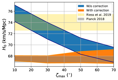
Figure 1: Hubble constant measurement uncertainty (1-$\sigma$) from 50 standard sirens as a function of the maximum viewing angle of the binaries. The Hubble constant used for the simulations is $67.4$ km/s/Mpc. If the maximum viewing angle is known, appropriate corrections can be applied (as described in Equation 1) and the uncertainty is the With correction band. In contrast, the W/o correction band shows the level of bias if the maximum viewing angle is unknown. For reference, the two horizontal bands denote the $H_{0}$ reported by Riess et al. Riess et al. (2019) ($74.03\pm 1.42$ km/s/Mpc) and Planck Aghanim et al. (2018) ($67.4\pm 0.5$ km/s/Mpc).

A possible way to determine the viewing angle selection effect is to analyze the viewing angle measurements from GWs for events with EM counterparts. We try to estimate $\zeta_{\rm max}$ in the first example above from the GW data of $N$ events {${\mathcal{D}_{1},\mathcal{D}_{2}...\mathcal{D}_{N}}$}:

$$p(\zeta_{\rm max}|\mathcal{D}_{1},\mathcal{D}_{2}...\mathcal{D}_{N})=\frac{p(\zeta_{\rm max})\displaystyle\prod_{k=1}^{N}p(\mathcal{D}_{k}|\zeta_{\rm max})}{\displaystyle\prod_{k=1}^{N}p(\mathcal{D}_{k})}$$

$$=p(\zeta_{\rm max})\displaystyle\prod_{k=1}^{N}\displaystyle\int_{0}^{\pi/2}\frac{p(\zeta|\mathcal{D}_{k})p(\zeta_{\rm max}|\zeta,\mathcal{D}_{k})}{p(\zeta_{\rm max})}d\zeta$$

$$=p(\zeta_{\rm max})\displaystyle\prod_{k=1}^{N}\displaystyle\int_{0}^{\pi/2}\frac{p(\zeta|\mathcal{D}_{k})p(\zeta|\zeta_{\rm max})}{p(\zeta)}d\zeta$$

$$=p(\zeta_{\rm max})\displaystyle\prod_{k=1}^{N}\frac{\displaystyle\int_{0}^{\zeta_{\rm max}}p(\zeta|\mathcal{D}_{k})d\zeta}{\displaystyle\int_{0}^{\zeta_{\rm max}}p(\zeta)d\zeta}.$$ (3)

The first line comes from the fact that each event are independent. The third line considers $p(\zeta_{\rm max}|\zeta,\mathcal{D}_{k})=p(\zeta_{\rm max}|\zeta)$, and the last line takes $p(\zeta|\zeta_{\rm max})\propto p(\zeta)$ for $\zeta<\zeta_{\rm max}$. Equation Systematic uncertainty of standard sirens from the viewing angle of binary neutron star inspirals can then be calculated from the GW-viewing angle posterior $p(\zeta|\mathcal{D}_{k})$, which is obtained by integrating the distance-inclination angle posterior $p(D_{L},\theta_{\mathrm{JN}}|\mathcal{D}_{k})$ over $D_{L}$, and the prior on viewing angle $p(\zeta)$ Schutz (2011). Without any prior on $\zeta_{\rm max}$, i.e. $p(\zeta_{\rm max})$ is taken as a constant, in Figure 2 we show the symmetric 1-$\sigma$ uncertainty of the $\zeta_{\rm max}$ posteriors (Equation Systematic uncertainty of standard sirens from the viewing angle of binary neutron star inspirals) as a function of the maximum EM viewing angle of 50 simulated BNSs.

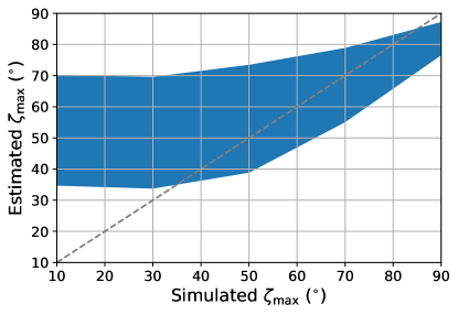
Figure 2: Maximum viewing angle $\zeta_{\rm max}$ estimated from 50 BNSs’ GW-viewing angle posteriors. The band denotes the symmetric $1\sigma$ uncertainty of the estimations, and the grey dashed line is the equal-axis line to guide the eye. Small simulated $\zeta_{\rm max}$ are not estimated accurately due to large uncertainty of the viewing angle posteriors.

We find that $\zeta_{\rm max}$ can only be confined to $\sim 20^{\circ}$ 1-$\sigma$ uncertainty. In addition, the estimated $\zeta_{\rm max}$ is biased for small $\zeta_{\rm max}$ because GW-viewing angle posteriors typically peak around $30^{\circ}$ with about $20^{\circ}$ uncertainty Chen et al. (2019). Small $\zeta_{\rm max}$ is therefore difficult to reconstruct even if all BNSs with observable EM counterparts are face-on/off.

Systematics from biased EM-constraint on viewing angle– Another possible bias comes from the interpretation of the EM observations. The angular dependency of EM emissions can be used to estimate the viewing angle of BNSs. However, lack of robust understanding of the EM emission model can lead to biased interpretation of the viewing angle.

Suppose the EM observations suggest a viewing angle of $\zeta_{\rm EM}$ with 1-$\sigma$ uncertainty of $\sigma_{\zeta}$, the EM likelihood in Equation 1 is then proportional to

$$p(\mathcal{D}_{\rm EM}|\vec{\Theta})\propto\begin{cases}\cal{N}(\theta_{\mathrm{JN}};\zeta_{\rm EM},\sigma_{\zeta})&\text{if}\,0\leq\theta_{\mathrm{JN}}\leq\pi/2\\ \cal{N}(\theta_{\mathrm{JN}};\pi-\zeta_{\rm EM},\sigma_{\zeta})&\text{if}\,\pi/2<\theta_{\mathrm{JN}}\leq\pi,\end{cases}$$ (4)

where $\cal{N}(\theta_{\mathrm{JN}};\zeta_{\rm EM},\sigma_{\zeta})$ denotes a normal distribution with mean $\zeta_{\rm EM}$ and standard deviation $\sigma_{\zeta}$ evaluated at $\theta_{\mathrm{JN}}$. Since Equation 4 provides constraint on the inclination angle and reduces the binary parameter space in Equation 1, the Hubble constant can be measured more precisely Chen et al. (2019). However, if the EM constraint on the viewing angle is off by

$$\Delta\zeta_{\rm sys}\equiv\zeta_{\rm EM}-\zeta_{\rm real},$$

where $\zeta_{\rm real}$ denotes the real viewing angle of the event, the $H_{0}$ measurements will be biased. For single event the bias in $H_{0}$ may not be obvious, because the statistical uncertainty in $H_{0}$ dominates the overall uncertainty. The bias will become clear after the $H_{0}$ posteriors are combined over multiple events. In Figure 3 we show the extent of overall bias in $H_{0}$ if the EM constraint on viewing angle is always off by $\Delta\zeta_{\rm sys}$ for 20 events.

When the viewing angles are overestimated (underestimated), the combined $H_{0}$ is overestimated (underestimated). Smaller $\sigma_{\zeta}$ affects the $H_{0}$ measurement more significantly for the same $\Delta\zeta_{\rm sys}$. Note that $\Delta\zeta_{\rm sys}$ is not necessarily a constant across different events. We choose a fixed bias $\Delta\zeta_{\rm sys}$ across 20 events only to reveal the average level of $H_{0}$ bias for a given $\Delta\zeta_{\rm sys}$, since the systematic uncertainty in $H_{0}$ is not expected to evolve with the total number of events. Combining 20 events instead of using a single event reduces the statistical fluctuations and manifest the systematic uncertainty in $H_{0}$. Our simulations map the systematic uncertainty in viewing angleinferred from EM observations to $H_{0}$ for the first time. From Figure 3, $\Delta\zeta_{\rm sys}$ has to be $\lesssim 10^{\circ}$ to be accurate enough to address the tension between Planck and the local distance ladders.

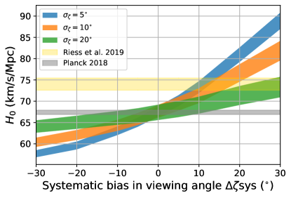
Figure 3: Hubble constant measurement uncertainty (1-$\sigma$) from 20 standard sirens as a function of the systematic bias in the binary viewing angle constrained by EM observations. Three different statistical uncertainties in the EM-constrained viewing angle ($\sigma_{\zeta}=5^{\circ},10^{\circ},20^{\circ}$) are shown. The Hubble constant used for the simulations is $67.4$ km/s/Mpc.

Next, we wonder if a comparison between the GW and EM measurement of the viewing angle will help disclosing the bias in EM interpretations. Suppose the viewing angle posteriors from GW and EM for a BNS are $\Upsilon(\zeta)$ and $\varepsilon(\zeta)$ respectively, we can define their difference as

$$\Delta\zeta_{\rm EM-GW}\equiv\displaystyle\int_{0}^{\pi/2}\int_{0}^{\pi/2}(\zeta_{2}-\zeta_{1})\times\Upsilon(\zeta_{1})\times\varepsilon(\zeta_{2})\,d\zeta_{1}d\zeta_{2}.$$ (5)

We find that the average of $\Delta\zeta_{\rm EM-GW}$ over 20 BNSs traces $\Delta\zeta_{\rm sys}$ with $1-\sigma$ uncertainty $>18^{\circ}$, as shown in Figure 4. This uncertainty of $\Delta\zeta_{\rm EM-GW}$ is larger than the required accuracy of $\zeta_{\rm EM}$ above, making it difficult to resolve the $H_{0}$ systematics from biased EM constraint.

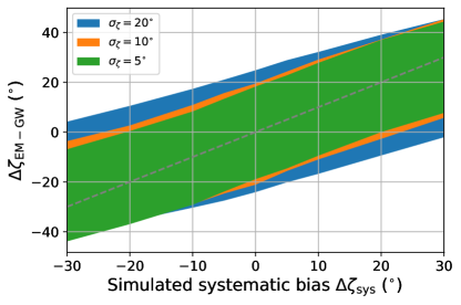
Figure 4: The average difference between EM- and GW-viewing angle posteriors $\Delta\zeta_{\rm EM-GW}$ for 20 BNSs with EM posteriors systematically off by $\Delta\zeta_{\rm sys}$. The $1-\sigma$ uncertainty of the difference for three EM posterior statistical uncertainties, $\sigma_{\zeta}=5^{\circ},10^{\circ},20^{\circ}$, are $18.5^{\circ}$, $20^{\circ}$, and $24^{\circ}$, respectively. The grey dashed line is the equal-axis line to guide the eye.

Discussion– In this paper we evaluate the extent of bias in $H_{0}$ as a result of the geometry of EM emissions from BNSs.

If the geometry affects the EM-observing probability, the selection effect can introduce a $\gtrsim 2\%$ bias on $H_{0}$. The example of maximum viewing angle we present may happen due to the choice of kilonova observing strategies or the sharp decline beyond a viewing angle for short GRB emission. Future studies of the jet structure of GRBs will be crucial to correct the selection effect for standard sirens. On the other hand, the example of continuous viewing angle selection is relevant for kilonova observations. Simulations show that edge-on BNSs are more difficult to localize Chen et al. (2019), and their kilonova emissions can be redder and dimmer Darbha and Kasen (2020). The resulting selection effects will depend on the telescopes, the observing strategies, and the observing conditions, so the overall effects can be subtle to estimate and correct.

Even if the selection effect is corrected, when the geometry of EM emissions is used to confine the BNSs’ viewing angle, the systematic uncertainty in viewing angle introduced by the EM interpretations has to be less than $\sim 10^{\circ}$. Since the binary rotational axis doesn’t have to be perfectly aligned with the major axis of EM emissions, and the geometry of EM emissions is unknown, to control the systematics of EM inferred viewing angle can be challenging. We also show that the comparison between EM- and GW-viewing angle measurements can help estimating the systematics, but the precision of the estimation may not be good enough to completely remove the bias.

We note that in reality other binary parameters will also affect the EM-observing probability. Therefore, more complete considerations of EM models and projections of EM-observing probability for future telescopes involved in the search for EM counterparts will result in more accurate estimation of the bias in $H_{0}$. Unlike the viewing angle measurement, some parameters, such as the mass, are estimated precise enough from GW signals for the selection effect to be taken care of. Overall, we find the selection over viewing angle discussed in this paper the most subtle and difficult to resolve.

If the viewing angle selection effect is significant, it is possible to reconstruct the selection by comparing the number of BNSs with and without EM counterparts. The distribution of viewing angle for BNSs detected in GWs is well-understood Schutz (2011). For example, it is known that about 15% of BNS detections have viewing angle larger than $60^{\circ}$. If 15% of BNSs miss counterparts, one explanation is that the maximum EM viewing angle is around $60^{\circ}$. A reconstruction of short GRB viewing angles using the inclination angles and distances of GW-GRB joint detections has been shown in  Farah et al. (2019). However, the reconstruction for kilonova will be more difficult since their EM-observing probability has more complicated dependency on the viewing angle. Such reconstruction can also be easily contaminated by other factors that affect the EM-observing probability and will have to be evaluated carefully.

Although our discussion focuses on BNSs, there are simulations suggesting stronger viewing angle dependency for EM counterparts of neutron star-black hole mergers Darbha and Kasen (2020). Therefore neutron star-black hole mergers can possibly introduce larger bias when they are used as standard sirens Vitale and Chen (2018).

We note that the standard siren method we discuss in this paper relies on the observations of EM counterparts and the measurements of the BNSs’ redshift. A complimentary approach of the standard siren method doesn’t require the EM counterparts but make use of galaxy catalogs may help deducing the systematics discussed in this paper. However, the galaxy catalogs approach will suffer from lower $H_{0}$ precision and other sources of systematics Chen et al. (2018); Gray et al. (2019), making it complicated to contribute to the issues.

Finally, the calibration uncertainty in GWs currently dominates the known systematic uncertainty for standard sirens. The bias in $H_{0}$ from calibration can be as large as $\sim 2\%$ Karki et al. (2016); Sun et al. (2020). Both of the systematics we find in this work can introduce $H_{0}$ bias larger than 2%. In summary, the systematic uncertainty from viewing angle for standard sirens can be a major challenge to resolve the tension in Hubble constant, and we look forward to future development to explore this topic.

acknowledgments– We acknowledge valuable discussions with Sylvia Biscoveanu, Michael Coughlin, Carl-Johan Haster, Daniel Holz, Kwan-Yeung Ken Ng, and Salvatore Vitale. HYC was supported by by the Black Hole Initiative at Harvard University, which is funded by grants from the John Templeton Foundation and the Gordon and Betty Moore Foundation to Harvard University.

References

- Schutz (1986) B. F. Schutz, Nature (London) 323, 310 (1986).
- Abbott et al. (2017a) B. Abbott et al. (LIGO Scientific, Virgo, 1M2H, Dark Energy Camera GW-E, DES, DLT40, Las Cumbres Observatory, VINROUGE, MASTER), Nature 551, 85 (2017a), eprint 1710.05835.
- Aghanim et al. (2018) N. Aghanim et al. (Planck) (2018), eprint 1807.06209.
- Riess et al. (2019) A. G. Riess, S. Casertano, W. Yuan, L. M. Macri, and D. Scolnic, Astrophys. J. 876, 85 (2019), eprint 1903.07603.
- Wong et al. (2019) K. C. Wong, S. H. Suyu, G. C. F. Chen, C. E. Rusu, M. Millon, D. Sluse, V. Bonvin, C. D. Fassnacht, S. Taubenberger, M. W. Auger, et al., arXiv e-prints arXiv:1907.04869 (2019), eprint 1907.04869.
- Pesce et al. (2020) D. W. Pesce, J. A. Braatz, M. J. Reid, A. G. Riess, D. Scolnic, J. J. Condon, F. Gao, C. Henkel, C. M. V. Impellizzeri, C. Y. Kuo, et al., Astrophys. J. Lett. 891, L1 (2020), eprint 2001.09213.
- Chen et al. (2018) H.-Y. Chen, M. Fishbach, and D. E. Holz, Nature (London) 562, 545 (2018), eprint 1712.06531.
- Abbott et al. (2017b) B. Abbott et al. (LIGO Scientific, Virgo, Fermi GBM, INTEGRAL, IceCube, AstroSat Cadmium Zinc Telluride Imager Team, IPN, Insight-Hxmt, ANTARES, Swift, AGILE Team, 1M2H Team, Dark Energy Camera GW-EM, DES, DLT40, GRAWITA, Fermi-LAT, ATCA, ASKAP, Las Cumbres Observatory Group, OzGrav, DWF (Deeper Wider Faster Program), AST3, CAASTRO, VINROUGE, MASTER, J-GEM, GROWTH, JAGWAR, CaltechNRAO, TTU-NRAO, NuSTAR, Pan-STARRS, MAXI Team, TZAC Consortium, KU, Nordic Optical Telescope, ePESSTO, GROND, Texas Tech University, SALT Group, TOROS, BOOTES, MWA, CALET, IKI-GW Follow-up, H.E.S.S., LOFAR, LWA, HAWC, Pierre Auger, ALMA, Euro VLBI Team, Pi of Sky, Chandra Team at McGill University, DFN, ATLAS Telescopes, High Time Resolution Universe Survey, RIMAS, RATIR, SKA South Africa/MeerKAT), Astrophys. J. Lett. 848, L12 (2017b), eprint 1710.05833.
- Holz and Hughes (2005) D. E. Holz and S. A. Hughes, Astrophys. J. 629, 15 (2005), eprint astro-ph/0504616.
- Dalal et al. (2006) N. Dalal, D. E. Holz, S. A. Hughes, and B. Jain, Phys. Rev. D 74, 063006 (2006), eprint astro-ph/0601275.
- Nissanke et al. (2013) S. Nissanke, D. E. Holz, N. Dalal, S. A. Hughes, J. L. Sievers, and C. M. Hirata, arXiv e-prints arXiv:1307.2638 (2013), eprint 1307.2638.
- Feeney et al. (2019) S. M. Feeney, H. V. Peiris, A. R. Williamson, S. M. Nissanke, D. J. Mortlock, J. Alsing, and D. Scolnic, Phys. Rev. Lett. 122, 061105 (2019), eprint 1802.03404.
- Karki et al. (2016) S. Karki, D. Tuyenbayev, S. Kandhasamy, B. P. Abbott, T. D. Abbott, E. H. Anders, J. Berliner, J. Betzwieser, C. Cahillane, L. Canete, et al., Review of Scientific Instruments 87, 114503 (2016), eprint 1608.05055.
- Sun et al. (2020) L. Sun, E. Goetz, J. S. Kissel, J. Betzwieser, S. Karki, A. Viets, M. Wade, D. Bhattacharjee, V. Bossilkov, P. B. Covas, et al., arXiv e-prints arXiv:2005.02531 (2020), eprint 2005.02531.
- Howlett and Davis (2020) C. Howlett and T. M. Davis, Mon. Not. R. Astron. Soc. 492, 3803 (2020), eprint 1909.00587.
- Mukherjee et al. (2019) S. Mukherjee, G. Lavaux, F. R. Bouchet, J. Jasche, B. D. Wand elt, S. M. Nissanke, F. Leclercq, and K. Hotokezaka, arXiv e-prints arXiv:1909.08627 (2019), eprint 1909.08627.
- Nicolaou et al. (2020) C. Nicolaou, O. Lahav, P. Lemos, W. Hartley, and J. Braden, Mon. Not. R. Astron. Soc. (2020), eprint 1909.09609.
- Abbott et al. (2019) B. Abbott et al. (LIGO Scientific, Virgo), Phys. Rev. X 9, 011001 (2019), eprint 1805.11579.
- Roberts et al. (2011) L. F. Roberts, D. Kasen, W. H. Lee, and E. Ramirez-Ruiz, Astrophys. J. Lett. 736, L21 (2011), eprint 1104.5504.
- Metzger (2017) B. D. Metzger, Living Reviews in Relativity 20, 3 (2017), eprint 1610.09381.
- Bulla (2019) M. Bulla, Mon. Not. R. Astron. Soc. 489, 5037 (2019), eprint 1906.04205.
- Darbha and Kasen (2020) S. Darbha and D. Kasen, arXiv e-prints arXiv:2002.00299 (2020), eprint 2002.00299.
- Sagués Carracedo et al. (2020) A. Sagués Carracedo, M. Bulla, U. Feindt, and A. Goobar, arXiv e-prints arXiv:2004.06137 (2020), eprint 2004.06137.
- Abbott et al. (2017c) B. Abbott et al. (LIGO Scientific, Virgo), Phys. Rev. Lett. 119, 161101 (2017c), eprint 1710.05832.
- Finstad et al. (2018) D. Finstad, S. De, D. A. Brown, E. Berger, and C. M. Biwer, Astrophys. J. Lett. 860, L2 (2018), eprint 1804.04179.
- Dhawan et al. (2020) S. Dhawan, M. Bulla, A. Goobar, A. Sagués Carracedo, and C. N. Setzer, Astrophys. J. 888, 67 (2020), eprint 1909.13810.
- Mooley et al. (2018) K. P. Mooley, A. T. Deller, O. Gottlieb, E. Nakar, G. Hallinan, S. Bourke, D. A. Frail, A. Horesh, A. Corsi, and K. Hotokezaka, Nature (London) 561, 355 (2018), eprint 1806.09693.
- Chen et al. (2019) H.-Y. Chen, S. Vitale, and R. Narayan, Physical Review X 9, 031028 (2019), eprint 1807.05226.
- Guidorzi et al. (2017) C. Guidorzi, R. Margutti, D. Brout, D. Scolnic, W. Fong, K. D. Alexander, P. S. Cowperthwaite, J. Annis, E. Berger, P. K. Blanchard, et al., Astrophys. J. Lett. 851, L36 (2017), eprint 1710.06426.
- Hotokezaka et al. (2019) K. Hotokezaka, E. Nakar, O. Gottlieb, S. Nissanke, K. Masuda, G. Hallinan, K. P. Mooley, and A. T. Deller, Nature Astronomy 3, 940 (2019), eprint 1806.10596.
- Abbott et al. (2018) B. Abbott et al. (KAGRA, LIGO Scientific, VIRGO), Living Rev. Rel. 21, 3 (2018), eprint 1304.0670.
- Mandel et al. (2019) I. Mandel, W. M. Farr, and J. R. Gair, Mon. Not. R. Astron. Soc. 486, 1086 (2019), eprint 1809.02063.
- Schutz (2011) B. F. Schutz, Classical and Quantum Gravity 28, 125023 (2011), eprint 1102.5421.
- Farah et al. (2019) A. Farah, R. Essick, Z. Doctor, M. Fishbach, and D. E. Holz, arXiv e-prints arXiv:1912.04906 (2019), eprint 1912.04906.
- Vitale and Chen (2018) S. Vitale and H.-Y. Chen, Phys. Rev. Lett. 121, 021303 (2018), eprint 1804.07337.
- Gray et al. (2019) R. Gray, I. Magaña Hernandez, H. Qi, A. Sur, P. R. Brady, H.-Y. Chen, W. M. Farr, M. Fishbach, J. R. Gair, A. Ghosh, et al., arXiv e-prints arXiv:1908.06050 (2019), eprint 1908.06050.