Non-lattice covering and quanitization of high dimensional sets

Abstract

The main problem considered in this paper is construction and theoretical study of efficient $n$-point coverings of a $d$-dimensional cube $[-1,1]^{d}$. Targeted values of $d$ are between 5 and 50; $n$ can be in hundreds or thousands and the designs (collections of points) are nested. This paper is a continuation of our paper us , where we have theoretically investigated several simple schemes and numerically studied many more. In this paper, we extend the theoretical constructions of us for studying the designs which were found to be superior to the ones theoretically investigated in us . We also extend our constructions for new construction schemes which provide even better coverings (in the class of nested designs) than the ones numerically found in us . In view of a close connection of the problem of quantization to the problem of covering, we extend our theoretical approximations and practical recommendations to the problem of construction of efficient quantization designs in a cube $[-1,1]^{d}$. In the last section, we discuss the problems of covering and quantization in a $d$-dimensional simplex; practical significance of this problem has been communicated to the authors by Professor Michael Vrahatis, a co-editor of the present volume.

1 Introduction

The problem of the main importance in this paper is the following problem of covering a cube $[-1,1]^{d}$ by $n$ balls. Let $Z_{1},\ldots,Z_{n}$ be a collection of points in $\mathbb{R}^{d}$ and ${\cal B}_{d}(Z_{j},r)=\{Z:\|Z-Z_{j}\|\leq r\}$ be the Euclidean balls of radius $r$ centered at $Z_{j}$ $(j=1,\ldots,n)$. The dimension $d$, the number of balls $n$ and their radius $r$ could be arbitrary.

We are interested in choosing the locations of the centers of the balls $Z_{1},\ldots,Z_{n}$ so that the union of the balls $\cup_{j}{\cal B}_{d}(Z_{j},r)$ covers the largest possible proportion of the cube $[-1,1]^{d}$. More precisely, we are interested in choosing a collection of points (called ‘design’) $\mathbb{Z}_{n}=\{Z_{1},\ldots,Z_{n}\}$ so that

$$C_{d}(\mathbb{Z}_{n},r):= ([-1,1]^{d}\cap{\cal B}_{d}(\mathbb{Z}_{n},r))/2^{d}$$vol (1)

is as large as possible (given $n$, $r$ and the freedom we are able to use in choosing $Z_{1},\ldots,Z_{n}$). Here ${\cal B}_{d}(\mathbb{Z}_{n},r)$ is the union of the balls

$${\cal B}_{d}(\mathbb{Z}_{n},r)=\bigcup_{j=1}^{n}{\cal B}_{d}(Z_{j},r)$$ (2)

and $C_{d}(\mathbb{Z}_{n},r)$ is the proportion of the cube $[-1,1]^{d}$ covered by ${\cal B}_{d}(\mathbb{Z}_{n},r)$. If $Z_{j}\in\mathbb{Z}_{n}$ are random then we shall consider $\mathbb{E}_{\mathbb{Z}_{n}}C_{d}(\mathbb{Z}_{n},r)$, the expected value of the proportion (1); for simplicity of notation, we will drop $\mathbb{E}_{\mathbb{Z}_{n}}$ while referring to $\mathbb{E}_{\mathbb{Z}_{n}}C_{d}(\mathbb{Z}_{n},r)$.

For a design $\mathbb{Z}_{n}$, its covering radius is defined by CR$(\mathbb{Z}_{n})=\max_{X\in{\cal C}_{d}}\min_{Z_{j}\in\mathbb{Z}_{n}}\|X-Z_{j}\|$. In computer experiments, covering radius is called minimax-distance criterion, see johnson1990minimax and pronzato2012design ; in the theory of low-discrepancy sequences, covering radius is called dispersion, see (niederreiter1992random, , Ch. 6).

The problem of optimal covering of a cube by $n$ balls has very high importance for the theory of global optimization and many branches of numerical mathematics. In particular, the $n$-point designs $\mathbb{Z}_{n}$ with smallest CR provide the following: (a) the $n$-point min-max optimal quadratures, see (sukharev2012minimax, , Ch.3,Th.1.1), (b) min-max $n$-point global optimization methods in the set of all adaptive $n$-point optimization strategies, see (sukharev2012minimax, , Ch.4,Th.2.1), and (c) worst-case $n$-point multi-objective global optimization methods in the set of all adaptive $n$-point algorithms, see vzilinskas2013worst . In all three cases, the class of (objective) functions is the class of Liptshitz functions, where the Liptshitz constant may be unknown. The results (a) and (b) are the celebrated results of A.G.Sukharev obtained in the late nineteen-sixties, see e.g. sukharev1971optimal , and (c) is a recent result of A. Žilinskas.

If $d$ is not small (say, $d>5$) then computation of the covering radius CR$(\mathbb{Z}_{n})$ for any non-trivial design $\mathbb{Z}_{n}$ is a very difficult computational problem. This explains why the problem of construction of optimal $n$-point designs with smallest covering radius is notoriously difficult, see for example recent surveys toth20172 ; toth1993packing . If $r=$CR$(\mathbb{Z}_{n})$, then $C_{d}(\mathbb{Z}_{n},r)$ defined in (1) is equal to 1, and the whole cube ${\cal C}_{d}$ gets covered by the balls. However, we are only interested in reaching the values like 0.95 or 0.99, when only a large part of the ball is covered.

We will say that ${\cal B}_{d}(\mathbb{Z}_{n},r)$ makes a $(1-\gamma)$-covering of $[-1,1]^{d}$ if

$$C_{d}(\mathbb{Z}_{n},r)=1-\gamma\,;$$ (3)

the corresponding value of $r$ will be called $(1\!-\!\gamma)$-covering radius and denoted $r_{1-\gamma}$ or $r_{1-\gamma}(\mathbb{Z}_{n})$. If $\gamma=0$ then the $(1\!-\!\gamma)$-covering becomes the full covering and 1-covering radius $r_{1}(\mathbb{Z}_{n})$ becomes the covering radius CR$(\mathbb{Z}_{n})$. The problem of construction of efficient designs with smallest possible $(1\!-\!\gamma)$-covering radius (with some small $\gamma>0$) will be referred to as the problem of weak covering.

Let us give two strong arguments why the problem of weak covering could be even more practically important than the problem of full covering.

• Numerical checking of weak covering (with an approximate value of $\gamma$) is straightforward while numerical checking of the full covering is practically impossible, if $d$ is large enough.

• For a given design $\mathbb{Z}_{n}$, $C_{d}(\mathbb{Z}_{n},r)$ defined in (1) and considered as a function of $r$, is a cumulative distribution function (c.d.f.) of the random variable (r.v.) $\varrho(U,\mathbb{Z}_{n})=\min_{Z_{i}\in\mathbb{Z}_{n}}\|U-Z_{i}\|$, where $U$ is a random vector uniformly distributed on $[-1,1]^{d}$, see (29) below. The covering radius CR$(\mathbb{Z}_{n})$ is the upper bound of this r.v. while in view of (3), $r_{1-\gamma}(\mathbb{Z}_{n})$ is the $(1-\gamma)$-quantile. Many practically important characteristics of designs such as quantization error considered in Section 7 are expressed in terms of the whole c.d.f. $C_{d}(\mathbb{Z}_{n},r)$ and their dependence on the upper bound CR$(\mathbb{Z}_{n})$ is marginal. As shown in Section 7.5, numerical studies indicate that comparison of designs on the base of their weak coverage properties is very similar to quantization error comparisons, but this may not be true for comparisons with respect to CR$(\mathbb{Z}_{n})$. This phenomenon is similar to the well-known fact in the theory of space covering by lattices (see an excellent book Conway and surveys toth20172 ; toth1993packing ), where best lattice coverings of space are often poor quantizers and vice-versa. Moreover, Figures 2-2 below show that CR$(\mathbb{Z}_{n})$ may give a totally inadequate impression about the c.d.f. $C_{d}(\mathbb{Z}_{n},r)$ and could be much larger than $r_{1-\gamma}(\mathbb{Z}_{n})$ with very small $\gamma>0$.

In Figures 2–2 we consider two simple designs for which we plot their c.d.f. $C_{d}(\cdot,r)$, black line, and also indicate the location of the $r_{1}$=CR and $r_{0.999}$ by vertical red and green line respectively. In Figure 2, we take $d=10$, $n=512$ and use a $2^{d-1}$ design of maximum resolution concentrated at the points $(\pm 1/2,\ldots,\pm 1/2)\in\mathbb{R}^{d}$ as design $\mathbb{Z}_{n}$; this design is a particular case of Design 4 of Section 8 and can be defined for any $d>2$. In Figure 2, we keep $d=10$ but take the full factorial $2^{d}$ design with $m=2^{d}$ points, again concentrated at the points $(\pm 1/2,\ldots,\pm 1/2)$; denote this design $\mathbb{Z}_{m}^{\prime}$.

For both designs, it is very easy to analytically compute their covering radii (for any $d>2$): CR$(\mathbb{Z}_{n})=\sqrt{d+8}/2$ and CR$(\mathbb{Z}_{m}^{\prime})=\sqrt{d}/2$; for $d=10$ this gives CR$(\mathbb{Z}_{n})\simeq 2.1213$ and CR$(\mathbb{Z}_{m}^{\prime})\simeq 1.58114.$ The values of $r_{0.999}$ are: $r_{0.999}(\mathbb{Z}_{n})\simeq 1.3465$ and $r_{0.999}(\mathbb{Z}_{m}^{\prime})\simeq 1.2708$. Their values have been computed using very accurate approximations developed in us1 ; we claim 3 correct decimal places in both values of $r_{0.999}$. We will return to this example in Section 2.1.

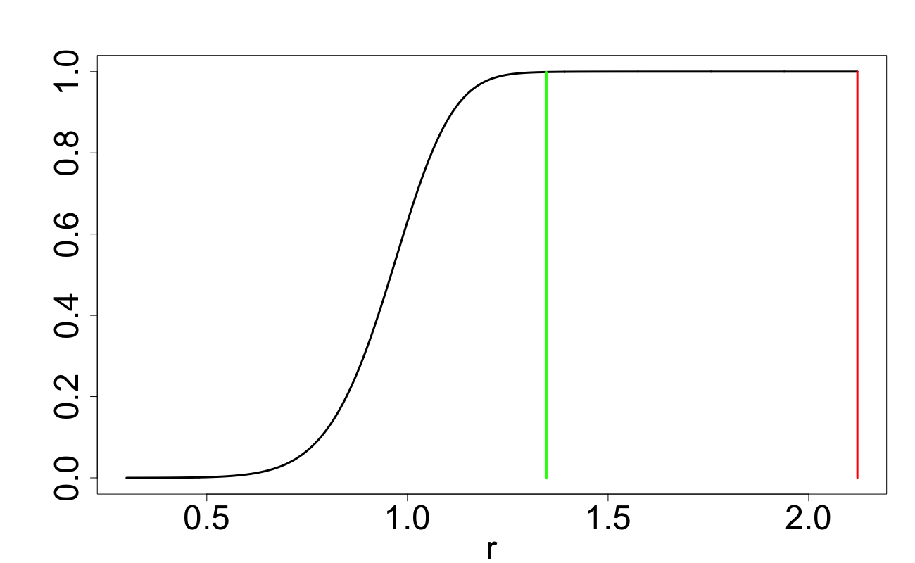
Figure 1: $C_{d}({\mathbb{Z}_{n}},r)$ with $r_{0.999}$ and $r_{1}$: $d=10$,
$\mathbb{Z}_{n}$ is a $2^{d-1}$-factorial design with $n=2^{d-1}$

Figure 2: $C_{d}({\mathbb{Z}_{m}^{\prime}},r)$ with $r_{0.999}$ and $r_{1}$: $d=10$,
$\mathbb{Z}_{m}$ is a $2^{d}$-factorial design

Of course, for any $\mathbb{Z}_{n}=\{Z_{1},\ldots,Z_{n}\}$ we can reach $C_{d}(\mathbb{Z}_{n},r)=1$ by means of increase of $r$. Likewise, for any given $r$ we can reach $C_{d}(\mathbb{Z}_{n},r)=1$ by sending $n\to\infty$. However, we are not interested in very large values of $n$ and try to get the coverage of the most part of the cube ${\cal C}_{d}$ with the radius $r$ as small as possible. We will keep in mind the following typical values of $d$ and $n$ which we will use for illustrating our results: $d=5,10,20,50$; $n=2^{k}$ with $k=6,\ldots,11$ (we have chosen $n$ as a power of 2 since this a favorable number for Sobol’s sequence (Design 3) as well as Design 4 defined in Section 8).

The structure of the rest of the paper is as follows. In Section 2 we discuss the concept of weak covering in more detail and introduce three generic designs which we will concentrate our attention on. In Sections 3, 4 and 5 we derive approximations for the expected volume of intersection the cube $[-1,1]^{d}$ with $n$ balls centred at the points of these designs. In Section 6, we provide numerical results showing that the developed approximations are very accurate. In Section 7, we derive approximations for the mean squared quantization error for chosen families of designs and numerically demonstrate that the developed approximations are very accurate. In Section 8, we numerically compare covering and quantization properties of different designs including scaled Sobol’s sequence and a family of very efficient designs defined only for very specific values of $n$. In Section 9 we try to answer the question raised by Michael Vrahatis by numerically investigating the importance of the effect of scaling points away from the boundary (we call it $\delta$-effect) for covering and quantization in a $d$-dimensional simplex. In Appendix, Section 10, we formulate a simple but important lemma about the distribution and moments of a certain random variable.

Our main theoretical contributions in this paper are:

• derivation of accurate approximations (16) and (22) for the probability $P_{U,\delta,\alpha,r}$ defined in (9);

• derivation of accurate approximations (18), (24) and (27) for the expected volume of intersection of the cube $[-1,1]^{d}$ with $n$ balls centred at the points of the selected designs;

• derivation of accurate approximations (32), (34) and (35) for the mean squared quantization error for the selected designs.

We have performed a large-scale numerical study and provided a number of figures and tables. The following are the key messages containing in these figures and tables.

• Figures 2–2: weak covering could be much more practically useful than the full covering;

• Figures 4–14: developed approximations for the probability $P_{U,\delta,\alpha,r}$ defined in (9) are very accurate;

• Figures 16–28: (a) developed approximations for $C_{d}(\mathbb{Z}_{n},r)$ are very accurate, (b) there is a very strong $\delta$-effect for all three types of designs, and (c) this $\delta$-effect gets stronger as $d$ increases;

• Tables 1 and 2 and Figures 30-30: smaller values of $\alpha$ are beneficial in Design 1 but Design 2 (where $\alpha=0$) becomes inefficient when $n$ gets close to $2^{d}$;

• Figures 32–44: developed approximations for the quantization error are very accurate and there is a very strong $\delta$-effect for all three types of designs used for quantization;

• Tables 3–4 and Figures 46-46: (a) Designs 2a and especially 2b provide very high quality coverage for suitable $n$, (b) properly $\delta$-tuned deterministic non-nested Design 4 provides superior covering, (c) coverage properties of $\delta$-tuned low-discrepancy sequences are much better than of the original low-discrepancy sequences, and (d) coverage properties of unadjusted low-discrepancy sequences is very low, if dimension $d$ is not small;

• Tables 5 and 6, Figures 48 and 48: very similar conclusions to the above but made with respect to the quantization error;

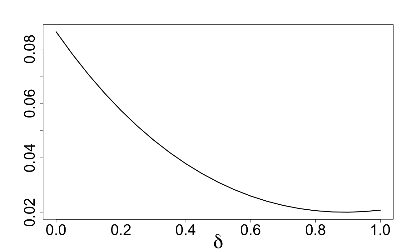
Figure 59: $\mathbb{E}\theta(\mathbb{Z}_{n})$ for Design S1: $d=20$, $n=1024$.

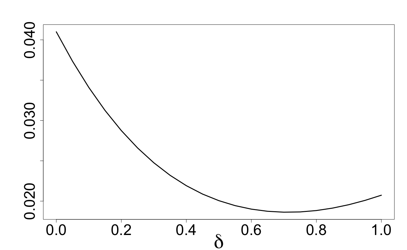
Figure 61: $\mathbb{E}\theta(\mathbb{Z}_{n})$ for Design S2: $d=20$, $n=1024$.

• Figures 52–62: the $\delta$-effect for covering and quantization schemes in a simplex is definitely present (this effect is more apparent in quantization) but it is much weaker than in a cube.

2 Weak covering

In this section, we consider the problem of weak covering defined and discussed in Section 1. The main characteristic of interest will be $C_{d}(\mathbb{Z}_{n},r)$, the proportion of the cube covered by the union of balls ${\cal B}_{d}(\mathbb{Z}_{n},r)$; it is defined in (1). We start the section with short discussion on comparison of designs based on their covering properties.

2.1 Comparison of designs from the view-point of weak covering

Two different designs will be differentiated in terms of covering performance as follows. Fix $d$ and let $\mathbb{Z}_{n}$ and $\mathbb{Z}_{n}^{\prime}$ be two $n$-point designs. For $(1-\gamma)$-covering with $\gamma\geq 0$, if $C_{d}(\mathbb{Z}_{n},r)=C_{d}(\mathbb{Z}_{n}^{\prime},r^{\prime})=1-\gamma$ and $r<r^{\prime}$, then the design $\mathbb{Z}_{n}$ provides a more efficient $(1-\gamma)$-covering and is therefore preferable. Moreover, the natural scaling for the radius is $r_{n}=n^{1/d}r$ and therefore we can compare an $n$-point design $\mathbb{Z}_{n}$ with an $m$-point design $\mathbb{Z}_{m}^{\prime}$ as follows: if $C_{d}(\mathbb{Z}_{n},r)=C_{d}(\mathbb{Z}_{m}^{\prime},r^{\prime})=1-\gamma$ and $n^{1/d}r<m^{1/d}r^{\prime}$, then we say that the design $\mathbb{Z}_{n}$ provides a more efficient $(1-\gamma)$-covering than the design $\mathbb{Z}_{m}^{\prime}$.

As an example, consider the designs used for plotting Figures 2 and 2 in Section 1: $\mathbb{Z}_{n}$ with $n=2^{d-1}$ and $\mathbb{Z}_{m}^{\prime}$ with $m=2^{d}$. For the full covering, we have for any $d$:

$$n^{1/d}r_{1}(\mathbb{Z}_{n})={2^{-1/d}\sqrt{d+8}}>{\sqrt{d}}=r_{1}(\mathbb{Z}_{m}^{\prime})m^{1/d}$$

so that the design $\mathbb{Z}_{m}^{\prime}$ is better than $\mathbb{Z}_{n}$ for the full covering for any $d$ and the difference between normalized covering radii is quite significant. For example, for $d=10$ we have

$$n^{1/d}r_{1}(\mathbb{Z}_{n})\simeq 3.9585\;\;\;{\rm and}\;\;r_{1}(\mathbb{Z}_{m}^{\prime})m^{1/d}\simeq 3.1623$$

For 0.999-covering, however, the situation is reverse, at least for $d=10$, where we have:

$$n^{1/d}r_{0.999}(\mathbb{Z}_{n})\simeq 2.5126<2.5416\simeq r_{1}(\mathbb{Z}_{m}^{\prime})m^{1/d}$$

and therefore the design $\mathbb{Z}_{n}$ is better for 0.999-covering than the design $\mathbb{Z}_{m}^{\prime}$ for $d=10$.

2.2 Reduction to the probability of covering a point by one ball

In the designs $\mathbb{Z}_{n}$, which are of most interest to us, the points $Z_{j}\in\mathbb{Z}_{n}$ are i.i.d. random vectors in $\mathbb{R}^{d}$ with a specified distribution. Let us show that for these designs, we can reduce computation of $C_{d}(\mathbb{Z}_{n},r)$ to the probability of covering $[-1,1]^{d}$ by one ball.

Let $Z_{1},\ldots,Z_{n}$ be i.i.d. random vectors in $\mathbb{R}^{d}$ and ${\cal B}_{d}(\mathbb{Z}_{n},r)$ be as defined in (2). Then, for given $U=(u_{1},\ldots,u_{d})\in\mathbb{R}^{d}$,

$$\mathbb{P}\left\{U\in{\cal B}_{d}(\mathbb{Z}_{n},r)\right\} = 1-\prod_{j=1}^{n}\mathbb{P}\left\{U\notin{\cal B}_{d}({Z}_{j},r)\right\}$$ (4)

$$= 1-\prod_{j=1}^{n}\left(1-\mathbb{P}\left\{U\in{\cal B}_{d}({Z}_{j},r)\right\}\right)$$

$$= 1-\bigg{(}1-\mathbb{P}_{{}_{Z}}\left\{\|U-{Z}\|\leq r\right\}\bigg{)}^{n}\,.$$

$C_{d}(\mathbb{Z}_{n},r)$, defined in (1), is simply

$$C_{d}(\mathbb{Z}_{n},r)=\mathbb{E}_{{}_{U}}\mathbb{P}\left\{U\in{\cal B}_{d}(\mathbb{Z}_{n},r)\right\}\,,$$ (5)

where the expectation is taken with respect to the uniformly distributed $U\in[-1,1]^{d}$. For numerical convenience, we shall simplify the expression (4) by using the approximation

$$(1-t)^{n}\simeq e^{-nt}\,,$$ (6)

where $t=\mathbb{P}_{{}_{Z}}\left\{\|U-{Z}\|\leq r\right\}$. This approximation is very accurate for small values of $t$ and moderate values of $nt$, which is always the case of our interest. Combining (4), (5) and (6), we obtain the approximation

$$C_{d}(\mathbb{Z}_{n},r)\simeq 1-\mathbb{E}_{{}_{U}}\exp(-n\cdot\mathbb{P}_{{}_{Z}}\left\{\|U-{Z}\|\leq r\right\})\,.$$ (7)

In the next section we will formulate three schemes that will be of theoretical interest in this paper. For each scheme and hence different distribution of $Z$, we shall derive accurate approximations for $\mathbb{P}_{{}_{Z}}\left\{\|U-{Z}\|\leq r\right\}$ and therefore, using (7), for $C_{d}(\mathbb{Z}_{n},r)$.

2.3 Designs of theoretical interest

The three designs that will be the focus of theoretical investigation in this paper are:

Design 1. $Z_{1},\ldots,Z_{n}\in\mathbb{Z}_{n}$ are i.i.d. random vectors on $[-\delta,\delta]^{d}$ with independent components distributed according to the following Beta${}_{\delta}(\alpha,\alpha)$ distribution with density:

$$p_{\alpha,\delta}(t)=\frac{(2\delta)^{1-2\alpha}}{\mbox{Beta$(\alpha,\alpha)$}}[\delta^{2}-t^{2}]^{\alpha-1}\,,\;\;-\delta<t<\delta\,,\text{ for some }\alpha>0\;\;{\rm and}\;0\leq\delta\leq 1.$$ (8)

Design 2a. $Z_{1},\ldots,Z_{n}\in\mathbb{Z}_{n}$ are i.i.d. random vectors obtained by sampling with replacement from the vertices of the cube $[-\delta,\delta]^{d}$.

Design 2b. $Z_{1},\ldots,Z_{n}\in\mathbb{Z}_{n}$ are random vectors obtained by sampling without replacement from the vertices of the cube $[-\delta,\delta]^{d}$.

All three designs above are nested so that $\mathbb{Z}_{n}\subset\mathbb{Z}_{n+1}$ for all eligible $n$. Designs 1 and 2a are defined for all $n=1,2,\ldots$ whereas Design 2b is defined for $n=1,2,\ldots,2^{d}$. The appealing property of any design whose points $Z_{i}$ are i.i.d. is the possibility of using (4); this is the case of Designs 1 and 2a. For Design 2b, we will need to make some adjustments, see Section 5.

In the case of $\alpha=1$ in Design 1, the distribution Beta${}_{\delta}(\alpha,\alpha)$ becomes uniform on $[-\delta,\delta]^{d}$. This case has been comprehensively studied in us with a number of approximations for $C_{d}(\mathbb{Z}_{n},r)$ being developed. The approximations developed in Section 3 are generalizations of the approximations of us . Numerical results of us indicated that Beta-distribution with $\alpha<1$ provides more efficient covering schemes; this explains the importance of the approximations of Section 3. Design 2a is the limiting form of Design 1 as $\alpha\rightarrow 0$. Theoretical approximations developed below for $C_{d}(\mathbb{Z}_{n},r)$ for Design 2a are, however, more precise than the limiting cases of approximations obtained for $C_{d}(\mathbb{Z}_{n},r)$ in case of Design 1. For numerical comparison, in Section 6 we shall also consider several other designs.

3 Approximation of $C_{d}(\mathbb{Z}_{n},r)$ for Design 1

As a result of (7), our main quantity of interest in this section will be the probability

$$P_{U,\delta,\alpha,r}:=\mathbb{P}_{{}_{Z}}\left\{\|U\!-\!Z\|\!\leq\!{r}\right\}\!=\!\mathbb{P}_{{}_{Z}}\left\{\|U\!-\!Z\|^{2}\leq{r^{2}}\right\}\!=\!\mathbb{P}\left\{\sum_{j=1}^{d}(u_{j}\!-\!z_{j})^{2}\leq{r}^{2}\right\}\;\;$$ (9)

in the case when $Z$ has the Beta-distribution with density (8). We shall develop a simple approximation based on the Central Limit Theorem (CLT) and then subsequently refine it using the general expansion in the CLT for sums of independent non-identical r.v.

3.1 Normal approximation for $P_{U,\delta,\alpha,r}$

Let $\eta_{u,\delta,\alpha}=(z-u)^{2}$, where $z$ has density (8). In view of Lemma 10, the r.v. $\eta_{u,\delta,\alpha}$ is concentrated on the interval $[(\max(0,\delta-|u|))^{2},(\delta+|u|)^{2}]$ and its first three central moments are:

$$\mu_{u}^{(1)} = \mathbb{E}\eta_{u,\delta,\alpha}=u^{2}+\frac{{{\delta}}^{2}}{2\,{\alpha}+1}\,,$$ (10)

$$\mu_{u}^{(2)} = {\rm var}(\eta_{u,\delta,\alpha})={\frac{4\delta^{2}}{2\,{\alpha}+1}}\left[u^{2}+{\frac{{{\delta}}^{2}{\alpha}}{\left(2\,{\alpha}+1\right)\left(2\,{\alpha}+3\right)}}\right]\,,$$ (11)

$$\mu_{u}^{(3)} = \mathbb{E}\left[\eta_{u,\delta,\alpha}-\mu_{u}^{(1)}\right]^{3}={\frac{48{\alpha}\,{{\delta}}^{4}}{\left(2\,{\alpha}+1\right)^{2}\left(2\,{\alpha}+3\right)}}\left[u^{2}+{\frac{{{\delta}}^{2}\left(2\,{\alpha}-1\right)}{3\left(2\,{\alpha}+5\right)\left(2\,{\alpha}+1\right)}}\right]\,.$$ (12)

For a given $U=(u_{1},\ldots,u_{d})\in\mathbb{R}^{d}$, consider the r.v.

$$\|U-Z\|^{2}=\sum_{i=1}^{d}\eta_{u_{i},\delta,\alpha}=\sum_{j=1}^{d}(u_{j}-z_{j})^{2}\,,$$

where we assume that $Z=(z_{1},\ldots,z_{d})$ is a random vector with i.i.d. components $z_{i}$ with density (8). From (10), its mean is

$$\mu=\mu_{d,\delta,\alpha,U}:=\mathbb{E}\|U-Z\|^{2}=\|U\|^{2}+\frac{{d{\delta}}^{2}}{2\,{\alpha}+1}\,.$$

Using independence of $z_{1},\ldots,z_{d}$ and (11), we obtain

$${\sigma}_{d,\delta,\alpha,U}^{2}:={\rm var}(\|U-Z\|^{2})={\frac{4\delta^{2}}{2\,{\alpha}+1}}\left[\|U\|^{2}+{\frac{{d{\delta}}^{2}{\alpha}}{\left(2\,{\alpha}+1\right)\left(2\,{\alpha}+3\right)}}\right]\,,$$

and from independence of $z_{1},\ldots,z_{d}$ and (12) we get

$${\mu}_{d,\delta,\alpha,U}^{(3)}:=\mathbb{E}\left[\|U-Z\|^{2}-\mu\right]^{3}=\sum_{j=1}^{d}\mu_{u_{j}}^{(3)}={\frac{48{\alpha}\,{{\delta}}^{4}}{\left(2\,{\alpha}+1\right)^{2}\left(2\,{\alpha}+3\right)}}\left[\|U\|^{2}+{\frac{{d{\delta}}^{2}\left(2\,{\alpha}-1\right)}{3\left(2\,{\alpha}+5\right)\left(2\,{\alpha}+1\right)}}\right]\,.\;\;\;\;\;\;$$

If $d$ is large enough then the conditions of the CLT for $\|U-Z\|^{2}$ are approximately met and the distribution of $\|U-Z\|^{2}$ is approximately normal with mean $\mu_{d,\delta,\alpha,U}$ and variance ${\sigma}_{d,\delta,\alpha,U}^{2}$. That is, we can approximate the probability $P_{U,\delta,\alpha,r}=\mathbb{P}_{{}_{Z}}\left\{\|U\!-\!Z\|\!\leq\!{r}\right\}$ by

$$P_{U,\delta,\alpha,r}\!\cong\Phi\left(\frac{{r}^{2}-\mu_{d,\delta,\alpha,U}}{{\sigma}_{d,\delta,\alpha,U}}\right)\,,$$ (13)

where $\Phi(\cdot)$ is the c.d.f. of the standard normal distribution:

$$\Phi(t)=\int_{-\infty}^{t}\varphi(v)dv\;\;{\rm with}\;\;\varphi(v)=\frac{1}{\sqrt{2\pi}}e^{-v^{2}/2}\,.$$

The approximation (13) has acceptable accuracy if the probability $P_{U,\delta,\alpha,r}$ is not very small; for example, it falls inside a $2\sigma$-confidence interval generated by the standard normal distribution. In the next section, we improve approximations (13) by using an Edgeworth-type expansion in the CLT for sums of independent non-identically distributed r.v.

3.2 Refined approximation for $P_{U,\delta,\alpha,r}$

General expansion in the central limit theorem for sums of independent non-identical r.v. has been derived by V.Petrov, see Theorem 7 in Chapter 6 in petrov2012sums , see also Proposition 1.5.7 in rao1987asymptotic . The first three terms of this expansion have been specialized by V.Petrov in Section 5.6 in petrov . By using only the first term in this expansion, we obtain the following approximation for the distribution function of $\|U-Z\|^{2}$:

$$\mathbb{P}\left(\frac{\|U-Z\|^{2}-\mu_{d,\delta,\alpha,U}}{\sigma_{d,\delta,\alpha,U}}\leq x\right)\cong\Phi(x)+\frac{\mu_{d,\delta,\alpha,U}^{(3)}}{6{\sigma}_{d,\delta,\alpha,U}^{3}}(1-x^{2})\varphi(x),$$ (14)

leading to the following improved form of (13):

$$P_{U,\delta,\alpha,r}\cong\Phi(t)+\frac{\alpha\delta\left[\|U\|^{2}+\frac{d\delta^{2}(2\alpha-1)}{3(2\alpha+5)(2\alpha+1)}\right]}{(2\alpha+3)(2\alpha+1)^{1/2}\left[\|U\|^{2}+\frac{d\delta^{2}\alpha}{(2\alpha+1)(2\alpha+3)}\right]^{3/2}}(1-t^{2})\varphi(t)\,,$$ (15)

where

$$t:=\frac{{r}^{2}-\mu_{d,\delta,\alpha,U}}{{\sigma}_{d,\delta,\alpha,U}}=\frac{\sqrt{2\alpha+1}(r^{2}-\|U\|^{2}-\frac{d\delta^{2}}{2\alpha+1})}{2\delta\sqrt{\|U\|^{2}+\frac{{d\delta^{2}\alpha}}{(2\alpha+1)(2\alpha+3)}}}\,.$$

For $\alpha=1$, we obtain

$$P_{U,\delta,\alpha,r}\cong\Phi(t)+\frac{\delta\left[\|U\|^{2}+{d\delta^{2}}/{63}\right]}{5\sqrt{3}\left[\|U\|^{2}+{d\delta^{2}}/{15}\right]^{3/2}}(1-t^{2})\varphi(t)\,\;\;{\rm with}\;\;t=\frac{\sqrt{3}(r^{2}-\|U\|^{2}-{d\delta^{2}}/{3})}{2\delta\sqrt{\|U\|^{2}+{{d\delta^{2}}}/{15}}}\,,$$

which coincides with formula (16) of us .

A very attractive feature of the approximations (13) and (15) is their dependence on $U$ through $\|U\|$ only. We could have specialized for our case the next terms in Petrov’s approximation but these terms no longer depend on $\|U\|$ only and hence the next terms are much more complicated. Moreover, adding one or two extra terms from Petrov’s expansion to the approximation (15) does not fix the problem entirely for all $U$, $\delta$, $\alpha$ and $r$. Instead, we propose a slight adjustment to the r.h.s of (15) to improve this approximation, especially for small dimensions. Specifically, we suggest the approximation

$$P_{U,\delta,\alpha,r}\cong\Phi(t)+c_{d,\alpha}\frac{\alpha\delta\left[\|U\|^{2}+\frac{d\delta^{2}(2\alpha-1)}{3(2\alpha+5)(2\alpha+1)}\right]}{(2\alpha+3)(2\alpha+1)^{1/2}\left[\|U\|^{2}+\frac{d\delta^{2}\alpha}{(2\alpha+1)(2\alpha+3)}\right]^{3/2}}(1-t^{2})\varphi(t)\,,$$ (16)

where $c_{d,\alpha}=1+{3}/{(\alpha d)}$.

Below, there are figures of two types. In Figures 4–4, we plot $P_{U,\delta,\alpha,r}$ over a wide range of $r$ ensuring that values of $P_{U,\delta,\alpha,r}$ lie in the whole range $[0,1]$. In Figures 6–8, we plot $P_{U,\delta,\alpha,r}$ over a much smaller range of $r$ with $P_{U,\delta,\alpha,r}$ lying roughly in the range $[0,0.02]$. For the purpose of using formula (4), we need to assess the accuracy of all approximations for smaller values of $P_{U,\delta,\alpha,r}$ and hence the second type of plots are more useful. In these figures, the solid black line depicts $P_{U,\delta,\alpha,r}$ obtained via Monte Carlo methods where for simplicity we have set $U=(1/2,1/2,\ldots,1/2)$ and $\delta=1/2$. Approximations (13) and (16) are depicted with a dotted blue and dash green line respectively. From numerous simulations and these figures, we can conclude the following. Whilst the basic normal approximation (13) seems adequate in the whole range of values of $r$, for particularly small probabilities, that we are most interested in, approximation (16) is much superior and appears to be very accurate for all values of $\alpha$.

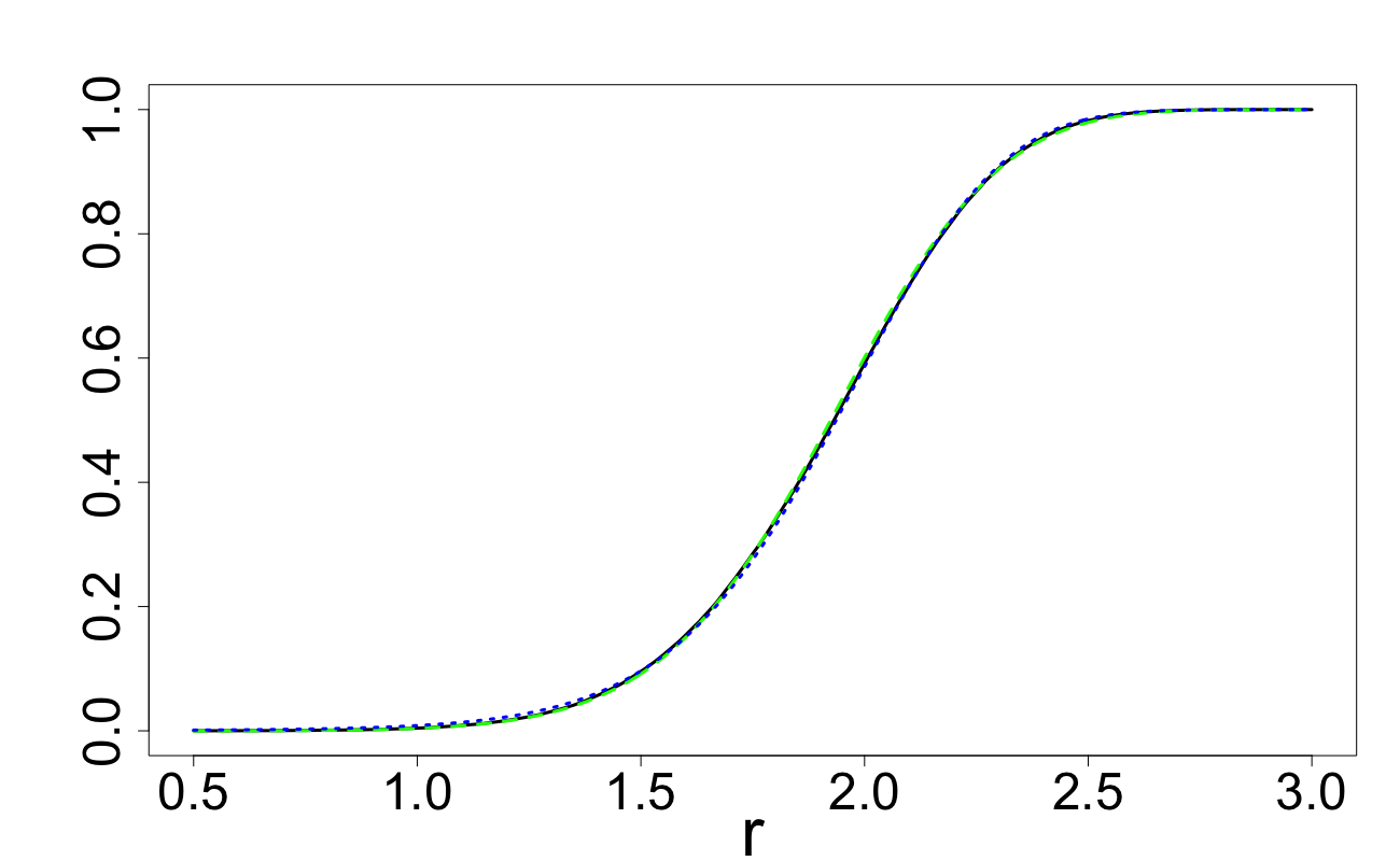
Figure 3: $P_{U,\delta,\alpha,r}$ and approximations: $d=10$,
$\alpha=0.5$.

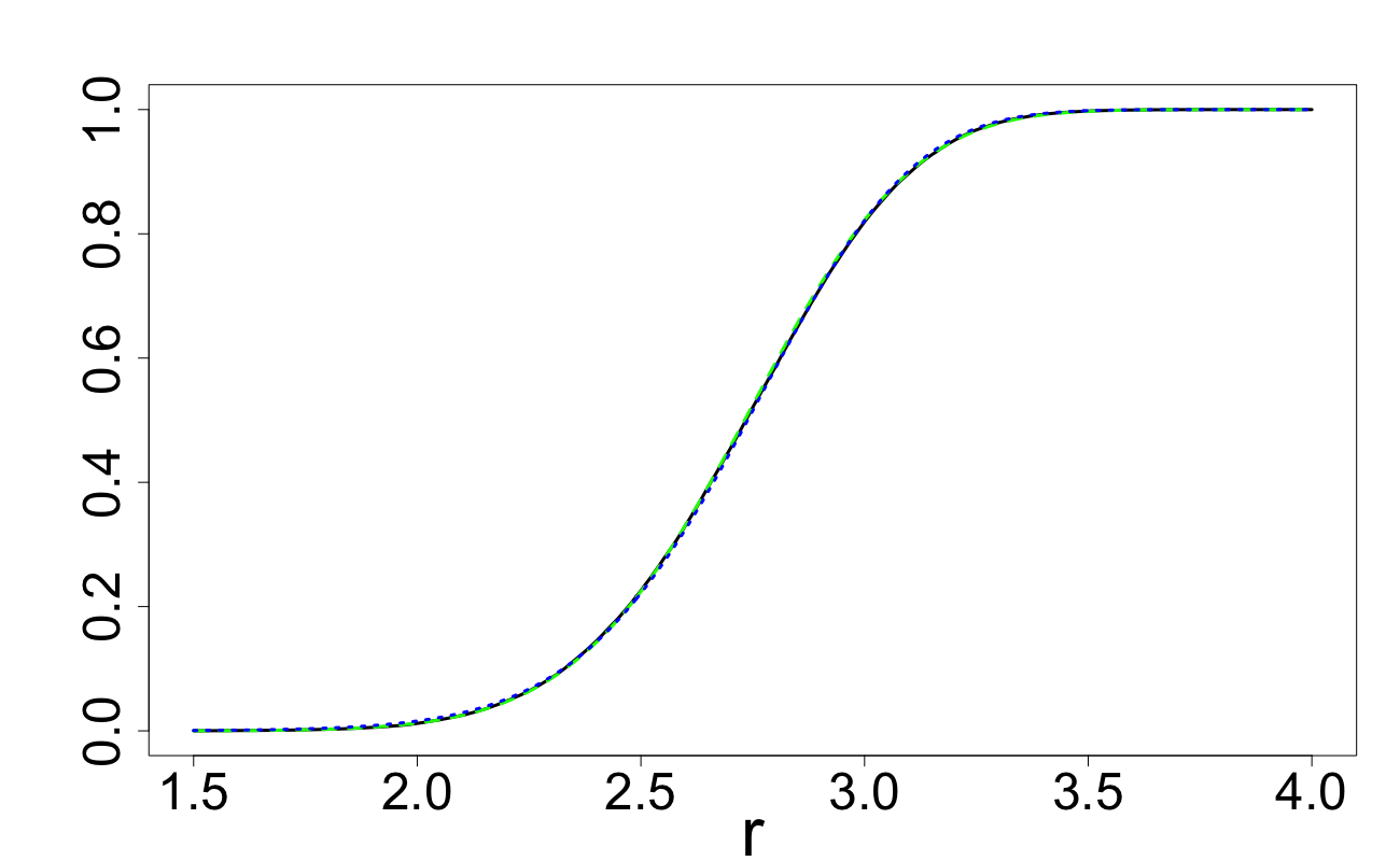
Figure 4: $P_{U,\delta,\alpha,r}$ and approximations: $d=20$,
$\alpha=0.5$.

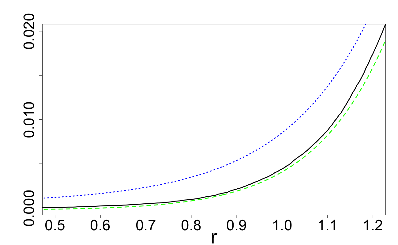
Figure 5: $P_{U,\delta,\alpha,r}$ and approximations: $d=10$,
$\alpha=0.5$.

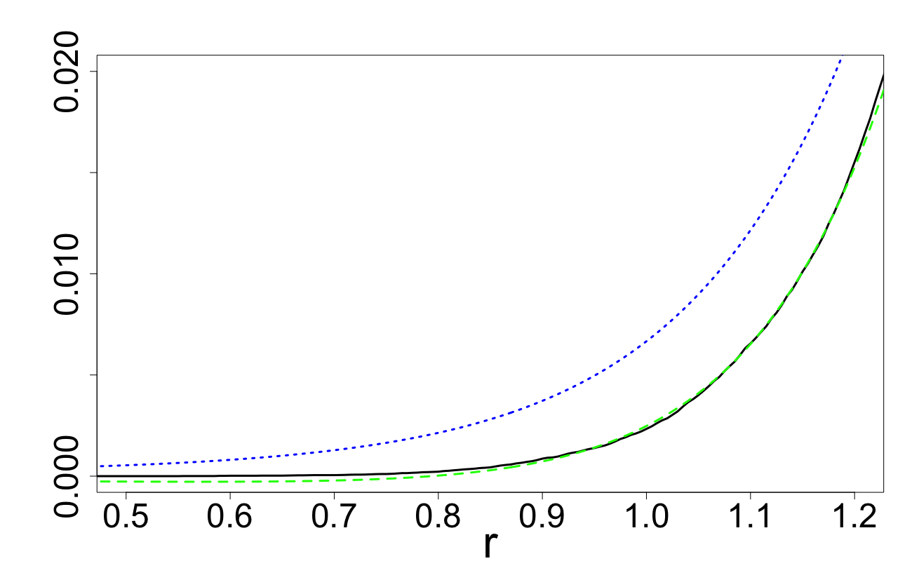
Figure 6: $P_{U,\delta,\alpha,r}$ and approximations: $d=10$,
$\alpha=1$.

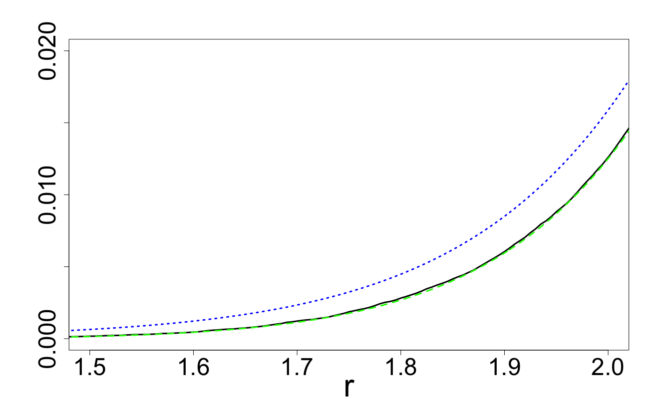
Figure 7: $P_{U,\delta,\alpha,r}$ and approximations: $d=20$,
$\alpha=0.5$.

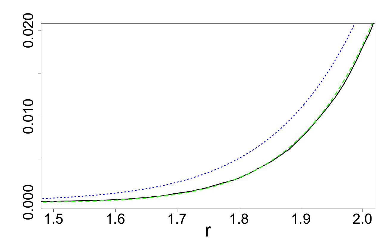
Figure 8: $P_{U,\delta,\alpha,r}$ and approximations: $d=20$,
$\alpha=1$.

3.3 Approximation for $C_{d}(\mathbb{Z}_{n},r)$ for Design 1

Consider now $C_{d}(\mathbb{Z}_{n},r)$ for Design 1, as expressed via $P_{U,\delta,\alpha,r}$ in (7). As $U$ is uniform on $[-1,1]^{d}$, $\mathbb{E}\|U\|^{2}=d/3$ and ${\rm var}(\|U\|^{2})={4d}/{45}.$ Moreover, if $d$ is large enough then $\|U\|^{2}=\sum_{j=1}^{d}u_{j}^{2}$ is approximately normal.

We will combine the expressions (7) with approximations (13) and (16) as well as with the normal approximation for the distribution of $\|U\|^{2}$, to arrive at two final approximations for $C_{d}(\mathbb{Z}_{n},r)$ that differ in complexity. If the original normal approximation (13) of $P_{U,\delta,\alpha,r}$ is used then we obtain:

$$C_{d}(\mathbb{Z}_{n},r)\simeq 1-\int_{-\infty}^{\infty}\psi_{1,\alpha}(s)\varphi(s)ds\;\;$$ (17)

with

$$\!\psi_{1,\alpha}(s)=\exp\left\{-n\Phi(c_{s})\right\},\,\ c_{s}=\frac{(2\alpha+1)^{1/2}\left(r^{2}\!-\!s^{\prime}\!-\!\frac{d\delta^{2}}{2\alpha+1}\right)}{2\delta\sqrt{s^{\prime}+\kappa}},\,\,s^{\prime}=s\sqrt{\frac{4d}{45}}+d/3,\,\,\kappa=\frac{d\delta^{2}\alpha}{(2\alpha\!+\!1)(2\alpha\!+\!3)}\,.\;\;$$

If the approximation (16) is used, we obtain:

$$C_{d}(\mathbb{Z}_{n},r)\simeq 1-\int_{-\infty}^{\infty}\psi_{2,\alpha}(s)\varphi(s)ds,\;\;\;\;$$ (18)

with

$$\psi_{2,\alpha}(s)=\exp\left\{-n\left(\Phi(c_{s})+c_{d,\alpha}\frac{\alpha\delta\left[s^{\prime}+\frac{d\delta^{2}(2\alpha-1)}{3(2\alpha+5)(2\alpha+1)}\right]}{(2\alpha+3)(2\alpha+1)^{1/2}\left[s^{\prime}+\kappa\right]^{3/2}}(1-c_{s}^{2})\varphi(c_{s})\right)\right\}\,.$$

For $\alpha=1$, we get

$$\psi_{2,1}(s)=\exp\left\{-n\left(\Phi(c_{s})+c_{d,\alpha}\frac{\delta\left[s^{\prime}+\frac{d\delta^{2}}{63}\right]}{5\sqrt{3}\left[s^{\prime}+\frac{d\delta^{2}}{15}\right]^{3/2}}(1-c_{s}^{2})\varphi(c_{s})\right)\right\}\,$$ (19)

and the approximation (18) coincides with the approximation (26) in us . The accuracy of approximations (17) and (18) will be assessed in Section 6.1.

4 Approximating $C_{d}(\mathbb{Z}_{n},r)$ for Design 2a

Our main quantity of interest in this section will be the probability $P_{U,\delta,0,r}$ defined in (9) in the case where components $z_{i}$ of the vector $Z=(z_{1},\ldots,z_{d})\in\mathbb{R}^{d}$ are i.i.d.r.v with ${\rm Pr}(z_{i}=\delta)={\rm Pr}(z_{i}=-\delta)=1/2$; this is a limiting case of $P_{U,\delta,\alpha,r}$ as $\alpha\to 0$.

4.1 Normal approximation for $P_{U,\delta,0,r}$

Using the same approach that led to approximation (13) in Section 3.1, the initial normal approximation for $P_{U,\delta,0,r}$ is:

$$P_{U,\delta,0,r}\!\cong\Phi\left(\frac{{r}^{2}-\mu_{d,\delta,U}}{{\sigma}_{d,\delta,U}}\right)\,,$$ (20)

where, from Lemma 10, we have

$$\mu_{d,\delta,U}=\|U\|^{2}+d{\delta}^{2}\,\,\text{ and }\,\,\ {\sigma}_{d,\delta,U}^{2}=4\delta^{2}\|U\|^{2}\,.$$

4.2 Refined approximation for $P_{U,\delta,0,r}$

From (38), we have ${\mu}_{d,\delta,\alpha,U}^{(3)}=0$ and therefore the last term in the rhs of (14) with $\alpha=0$ is no longer present. By taking an additional term in the general expansion, see V.Petrov in Section 5.6 in petrov , we obtain the following approximation for the distribution function of $\|U-Z\|^{2}$:

$$\mathbb{P}\left(\frac{\|U-Z\|^{2}-\mu_{d,\delta,U}}{\sigma_{d,\delta,U}}\leq x\right)\cong\Phi(x)-(x^{3}-3x)\frac{\kappa_{d,\delta,0,U}^{(4)}}{24{\sigma}_{d,\delta,0,U}^{4}}\varphi(x),$$ (21)

where $\kappa_{d,\delta,0,U}^{(4)}$ is the sum of $d$ fourth cumulants of the centred r.v. $(z-u)^{2}$, where $z$ is concentrated at two points $\pm\delta$ with ${\rm Pr}(z=\pm\delta)=1/2$. From (38),

$$\kappa_{d,\delta,0,U}^{(4)}:=\sum_{j=1}^{d}(\mu_{u_{j}}^{(4)}-3[\mu_{u_{j}}^{(2)}]^{2})=-32\delta^{4}\sum_{i=1}^{d}u_{i}^{4}\,.$$

Unlike (14), the rhs of (21) does not depends solely on $\|U\|^{2}$. However, the quantities $\|U\|^{2}$ and $\sum_{i=1}^{d}u_{i}^{4}$ are strongly correlated; one can show that for all $d$

$${\rm corr}\left(\|U\|^{2},\sum_{i=1}^{d}u_{i}^{4}\right)=\frac{3\sqrt{5}}{7}\cong 0.958\,.$$

This suggests (by rounding the correlation above to 1) the following approximation:

$$\sum_{i=1}^{d}u_{i}^{4}\cong\frac{4\sqrt{d}}{15}\left(\frac{\|U\|^{2}-d/3}{\sqrt{\frac{4d}{45}}}\right)+\frac{d}{5}\,.$$

With this approximation, the rhs of (21) depends only on $\|U\|^{2}$. As a result, the following refined form of (20) is:

$$P_{U,\delta,0,r}\cong\Phi(t)+(t^{3}-3t)\frac{2(\|U\|^{2}-d/3)/\sqrt{5}+d/5}{12\|U\|^{4}}\varphi(t),$$

where

$$t:=\frac{{r}^{2}-\mu_{d,\delta,0,U}}{{\sigma}_{d,\delta,0,U}}=\frac{(r^{2}-\|U\|^{2}-d\delta^{2})}{2\delta\|U\|}\,.$$

Similarly to approximation (16), we propose a slight adjustment to the r.h.s of the approximation above:

$$P_{U,\delta,0,r}\cong\Phi(t)+\left(1+\frac{3}{d}\right)(t^{3}-3t)\frac{2(\|U\|^{2}-d/3)/\sqrt{5}+d/5}{12\|U\|^{4}}\varphi(t).$$ (22)

In the same style as at the end of Section 3.2, below there are figures of two types. In Figures 10–10, we plot $P_{U,\delta,0,r}$ over a wide range of $r$ ensuring that values of $P_{U,\delta,0,r}$ lie in the range $[0,1]$. In Figures 12–14, we plot $P_{U,\delta,0,r}$ over a much smaller range of $r$ with $P_{U,\delta,0,r}$ lying in the range $[0,0.02]$. In these figures, the solid black line depicts $P_{U,\delta,\alpha,r}$ obtained via Monte Carlo methods where we have set $\delta=1/2$ and $U$ is a point sampled uniformly on $[-1,1]^{d}$; for reproducibility, in the caption of each figure we state the random seed used in R. Approximations (20) and (22) are depicted with a dotted blue and dash green line respectively. From these figures, we can conclude the same outcome as in Section 3.2. Whilst the approximation (20) is rather good overall, for small probabilities the approximation (22) is much superior and is very accurate. Note that since random vectors $Z_{j}$ are taking values on a finite set, which is the set of points $(\pm\delta,\ldots,\pm\delta)$, the probability $P_{U,\delta,0,r}$ considered as a function of $r$, is a piece-wise constant function.

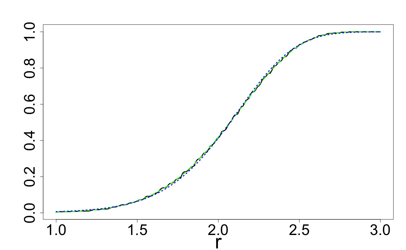
Figure 9: $P_{U,\delta,0,r}$ and approximations: $d=10$,
$seed=10$.

Figure 10: $P_{U,\delta,0,r}$ and approximations: $d=20$,
$seed=10$.

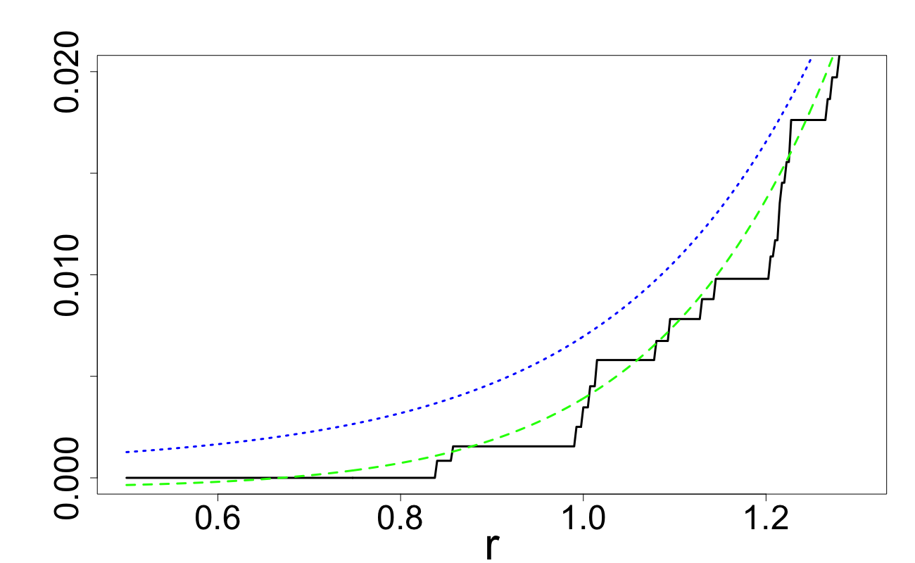
Figure 11: $P_{U,\delta,0,r}$ and approximations: $d=10$,
$seed=10$.

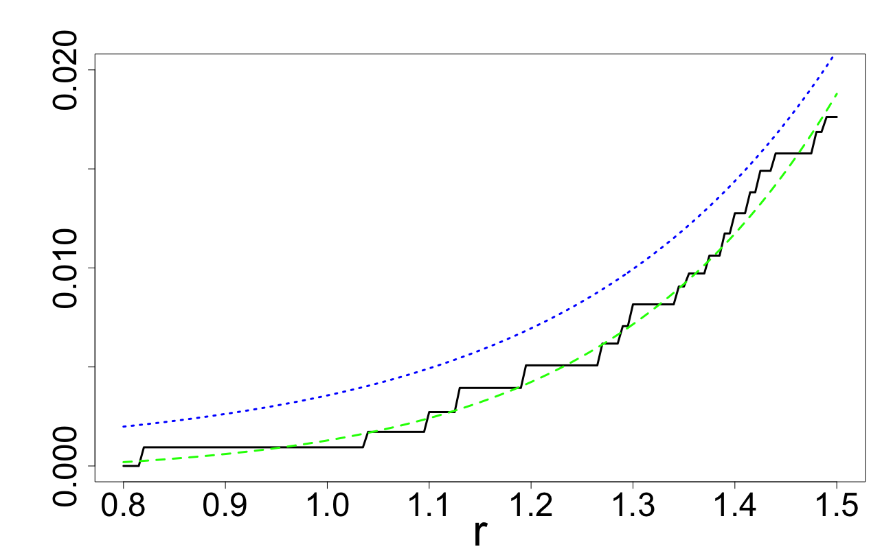
Figure 12: $P_{U,\delta,0,r}$ and approximations: $d=10$,
$seed=15$.

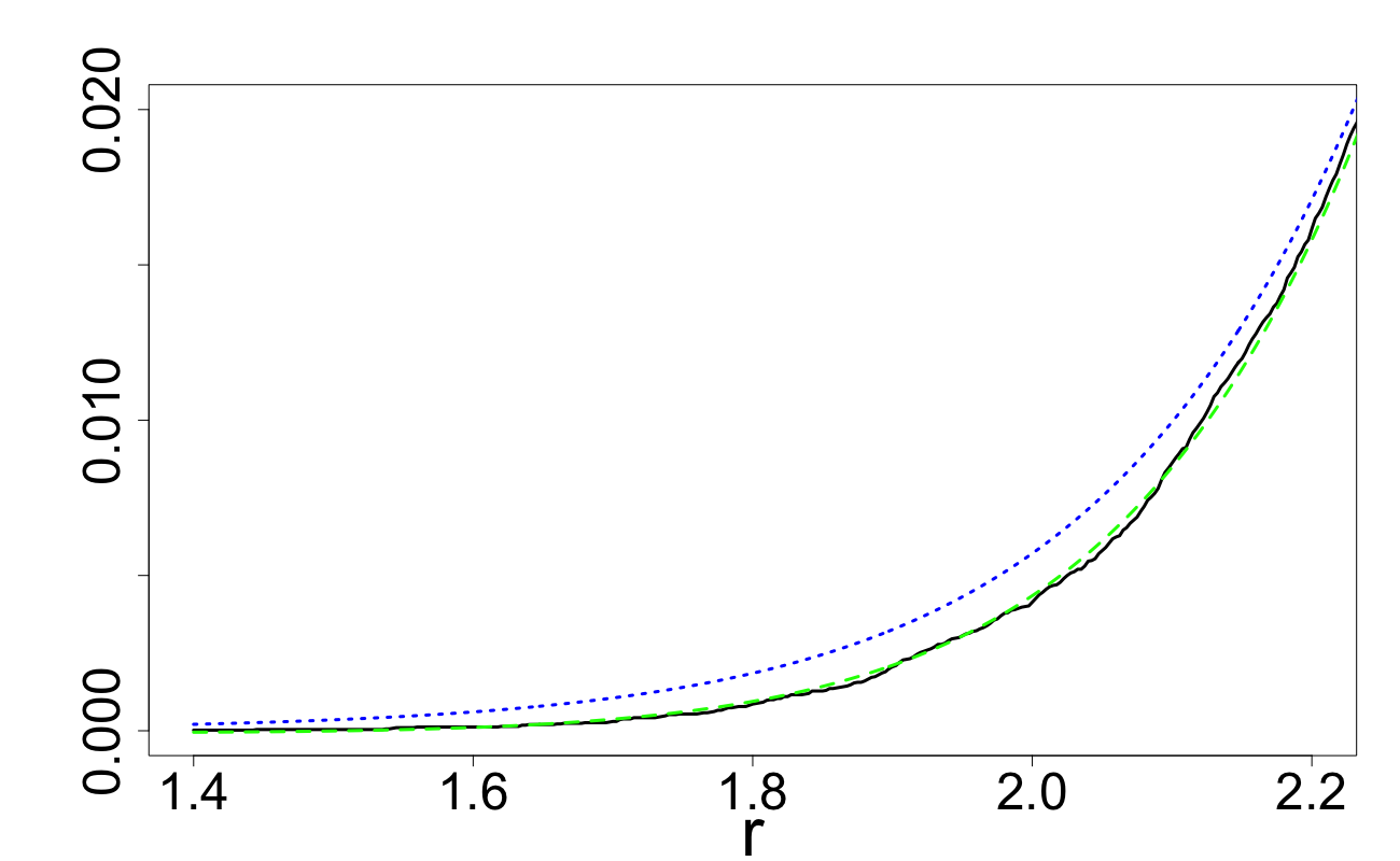
Figure 13: $P_{U,\delta,0,r}$ and approximations: $d=20$,
$seed=10$.

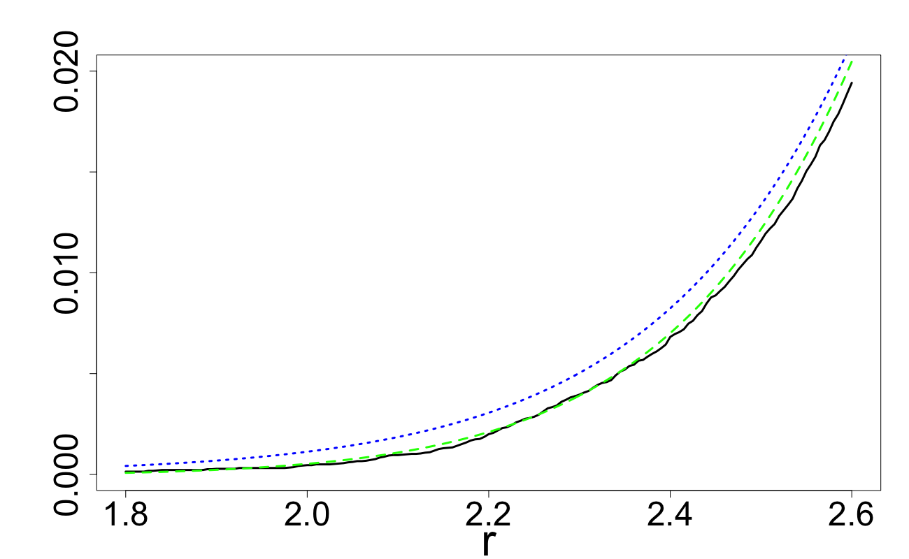
Figure 14: $P_{U,\delta,0,r}$ and approximations: $d=20$,
$seed=15$.

4.3 Approximation for $C_{d}(\mathbb{Z}_{n},r)$

Consider now $C_{d}(\mathbb{Z}_{n},r)$ for Design 2a, as expressed via $P_{U,\delta,\alpha,r}$ in (7). Using the normal approximation for $\|U\|^{2}$ as made in the beginning of Section 3.3, we will combine the expressions (7) with approximations (20) and (22) to arrive at two approximations for $C_{d}(\mathbb{Z}_{n},r)$ that differ in complexity.

If the original normal approximation (20) of $P_{U,\delta,0,r}$ is used then we obtain:

$$C_{d}(\mathbb{Z}_{n},r)\simeq 1-\int_{-\infty}^{\infty}\psi_{3,n}(s)\varphi(s)ds,\;\;$$ (23)

with

$$\psi_{3,n}(s)=\exp\left\{-n\Phi(c_{s})\right\}\,,\,\,\,\,c_{s}=\frac{\left(r^{2}-s^{\prime}-{d\delta^{2}}\right)}{2\delta\sqrt{s^{\prime}}},\,\,s^{\prime}=s\sqrt{\frac{4d}{45}}+d/3\,\,.$$

If the approximation (22) is used, we obtain:

$$C_{d}(\mathbb{Z}_{n},r)\simeq 1-\int_{-\infty}^{\infty}\psi_{4,n}(s)\varphi(s)ds,\;\;\;\;$$ (24)

with

$$\psi_{4,n}(s)=\exp\left\{-n\left(\Phi(c_{s})+\left(1+\frac{3}{d}\right)(c_{s}^{3}-3c_{s})\frac{2(s^{\prime}-d/3)/\sqrt{5}+d/5}{12(s^{\prime})^{2}}\varphi(c_{s})\right)\right\}\,.$$ (25)

and

$$\,\ c_{s}=\frac{\left(r^{2}-s^{\prime}-{d\delta^{2}}\right)}{2\delta\sqrt{s^{\prime}}},\,\,s^{\prime}=s\sqrt{\frac{4d}{45}}+d/3\,\,.$$

The accuracy of approximations (23) and (24) will be assessed in Section 6.1.

5 Approximating $C_{d}(\mathbb{Z}_{n},r)$ for Design 2b

Designs whose points $Z_{i}$ have been sampled from a finite discrete set without replacement have dependence, for example Design 2b, and therefore formula (4) cannot be used.

In this section, we suggest a way of modifying the approximations developed in Section 4 for Design 2a. This will amount to approximating sampling without replacement by a suitable sampling with replacement.

5.1 Establishing a connection between sampling with and without replacement: general case

Let $\cal{S}$ be a discrete set with $k$ distinct elements, where $k$ is reasonably large. In case of Design 2b, the set $\cal{S}$ consists of $k=2^{d}$ vertices of the cube $[-\delta,\delta]^{d}$. Let $\mathbb{Z}_{n}=\{Z_{1},\ldots,Z_{n}\}$ denote an $n-$point design whose points $Z_{i}$ have been sampled without replacement from $\cal{S}$; $n<k$. Also, let $\mathbb{Z}_{m}^{\prime}=\{Z_{1}^{\prime},\ldots,Z_{m}^{\prime}\}$ denote an associated $m-$point design whose points $Z_{i}^{\prime}$ are sampled with replacement from the same discrete set $\cal{S}$; $Z_{1}^{\prime},\ldots,Z_{m}^{\prime}$ are i.i.d. random vectors with values in $\cal{S}$. Our aim in this section is to establish an approximate correspondence between $n$ and $m$.

When sampling $m$ times with replacement, denote by $X_{i}$ the number of times the $i^{th}$ element of $\cal{S}$ appears. Then the vector $(X_{1},X_{2},\ldots,X_{k})$ has the multinomial distribution with number of trials $m$ and event probabilities $(1/k,1/k,\ldots,1/k)$ with each individual $X_{i}$ having the Binomial distribution $Binomial(m,1/k)$. Since ${\rm corr}(X_{i},X_{j})=-1/k^{2}$ when $i\neq j$, for large $k$ the correlation between random variables $X_{1},X_{2},\ldots,X_{k}$ is very small and will be neglected. Introduce the random variables:

$$Y_{i}=\begin{cases}1,\text{ if }X_{i}=0\\ 0,\text{ if }X_{i}>0.\end{cases}$$

Then the random variable $N_{0}=\sum_{i=1}^{k}Y_{i}$ represents the number of elements of $\cal{S}$ not selected. Given the weak correlation between $X_{i}$, we approximately have $N_{0}\sim Binomial(k,P(X_{1}=0))$. Using the fact $P(X_{1}=0)=(1-1/k)^{m}$, the expected number of unselected elements when sampling with replacement is approximately $\;\mathbb{E}N_{0}\cong k(1-1/k)^{m}\,.$ Since, when sampling without replacement from $\cal S$ we have chosen $N_{0}=k-n$ elements, to choose the value of $m$ we equate $\mathbb{E}N_{0}$ to $k-n$. By solving the equation

$$k-n=k\left(1-\frac{1}{k}\right)^{m}\;\;\;\left[\;\cong\;\mathbb{E}N_{0}\;\right]$$

for $m$ we obtain

$$m=\frac{\log(k-n)-\log(k)}{\log(k-1)-\log(k)}\,.$$ (26)

5.2 Approximation of $C_{d}(\mathbb{Z}_{n},r)$ for Design 2b.

Consider now $C_{d}(\mathbb{Z}_{n},r)$ for Design 2b. By applying the approximation developed in the previous section, the quantity $C_{d}(\mathbb{Z}_{n},r)$ can be approximated by $C_{d}(\mathbb{Z}_{m},r)$ for Design 2a with $m$ given in (26):

Approximation of $C_{d}(\mathbb{Z}_{n},r)$ for Design 2b. We approximate it by $C_{d}(\mathbb{Z}_{m},r)$ where $m$ is given in (26) and $C_{d}(\mathbb{Z}_{m},r)$ is approximated by (24) with $n$ substituted by $m$ from (26).

Specifying this, we obtain:

$$C_{d}(\mathbb{Z}_{n},r)\simeq 1-\int_{-\infty}^{\infty}\psi_{4,m}(s)\varphi(s)ds,\;\;\;\;$$ (27)

where

$$m=m_{n,d}=\frac{\log(2^{d}-n)-d\log(2)}{\log(2^{d}-1)-d\log(2)}\,$$ (28)

and the function $\psi_{4,\cdot}(\cdot)$ is defined in (25). The accuracy of the approximation (27) will be assessed in Section 6.1.

6 Numerical study

6.1 Assessing accuracy of approximations of $C_{d}(\mathbb{Z}_{n},r)$ and studying their dependence on $\delta$

In this section, we present the results of a large-scale numerical study assessing the accuracy of approximations (17), (18), (23), (24) and (27). In Figures 16–28, by using a solid black line we depict $C_{d}(\mathbb{Z}_{n},r)$ obtained by Monte Carlo methods, where the value of $r$ has been chosen such that the maximum coverage across $\delta$ is approximately $0.9$. In Figures 16–20, dealing with Design 1, approximations (17) and (18) are depicted with a dotted blue and dashed green lines respectively. In Figures 22–24 (Design 2a) approximations (23) and (24) are illustrated with a dotted blue and dashed green lines respectively. In Figures 26–28 (Design 2b) the dashed green line depicts approximation (27). From these figures, we can draw the following conclusions.

• Approximations (18) and (24) are very accurate across all values of $\delta$ and $\alpha$. This is particularly evident for $d=20,50$.

• Approximations (17) and (23) are accurate only for very large values of $d$, like $d=50$.

• Approximation (24) is generally accurate. For $\delta$ close to one (for such values of $\delta$ the covering is very poor) and $n$ close to $2^{d}$ this approximation begins to worsen, see Figures 26 and 28.

• A sensible choice of $\delta$ can dramatically increase the coverage proportion $C_{d}(\mathbb{Z}_{n},r)$. This effect, which we call ‘$\delta$-effect’, is evident in all figures and is very important. It gets much stronger as $d$ increases.

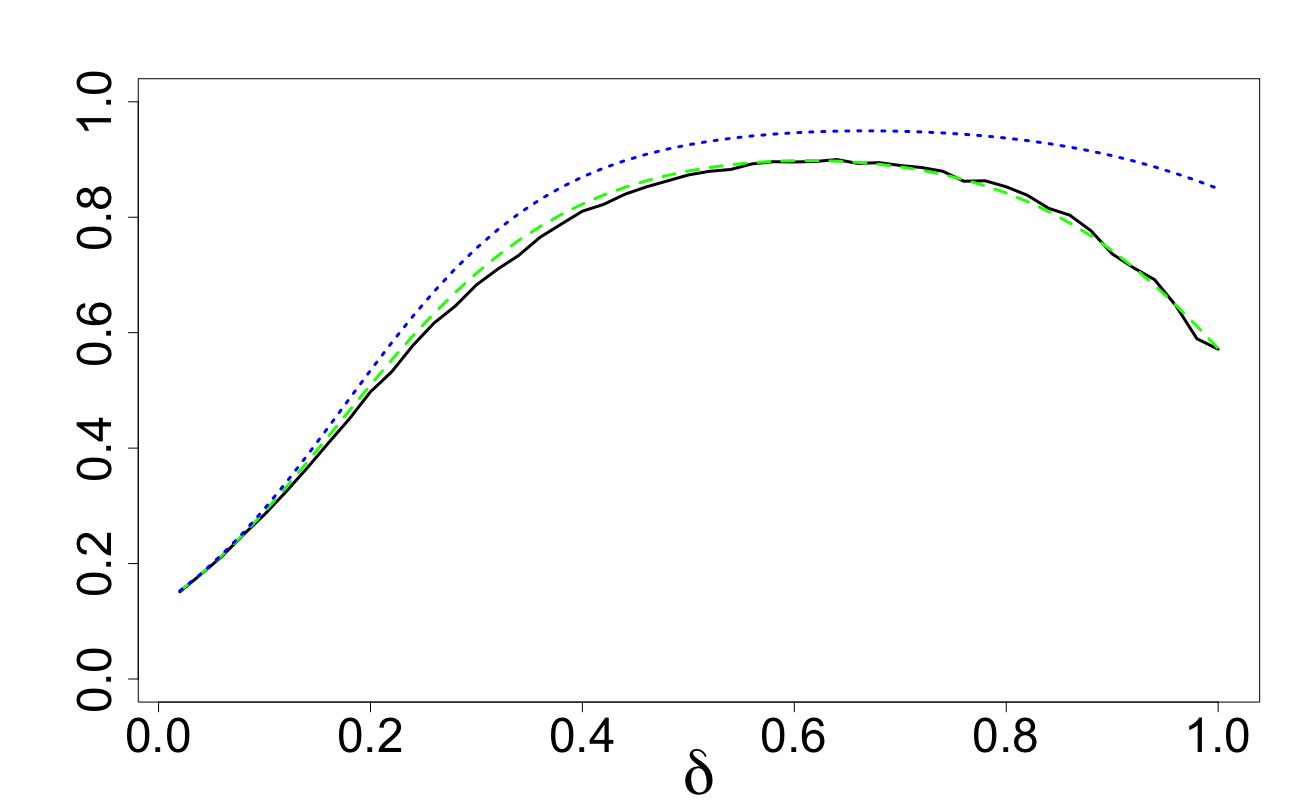
Figure 15: Design 1: $C_{d}(\mathbb{Z}_{n},r)$ and approximations;
$d=10,\alpha=0.5,n=128$.

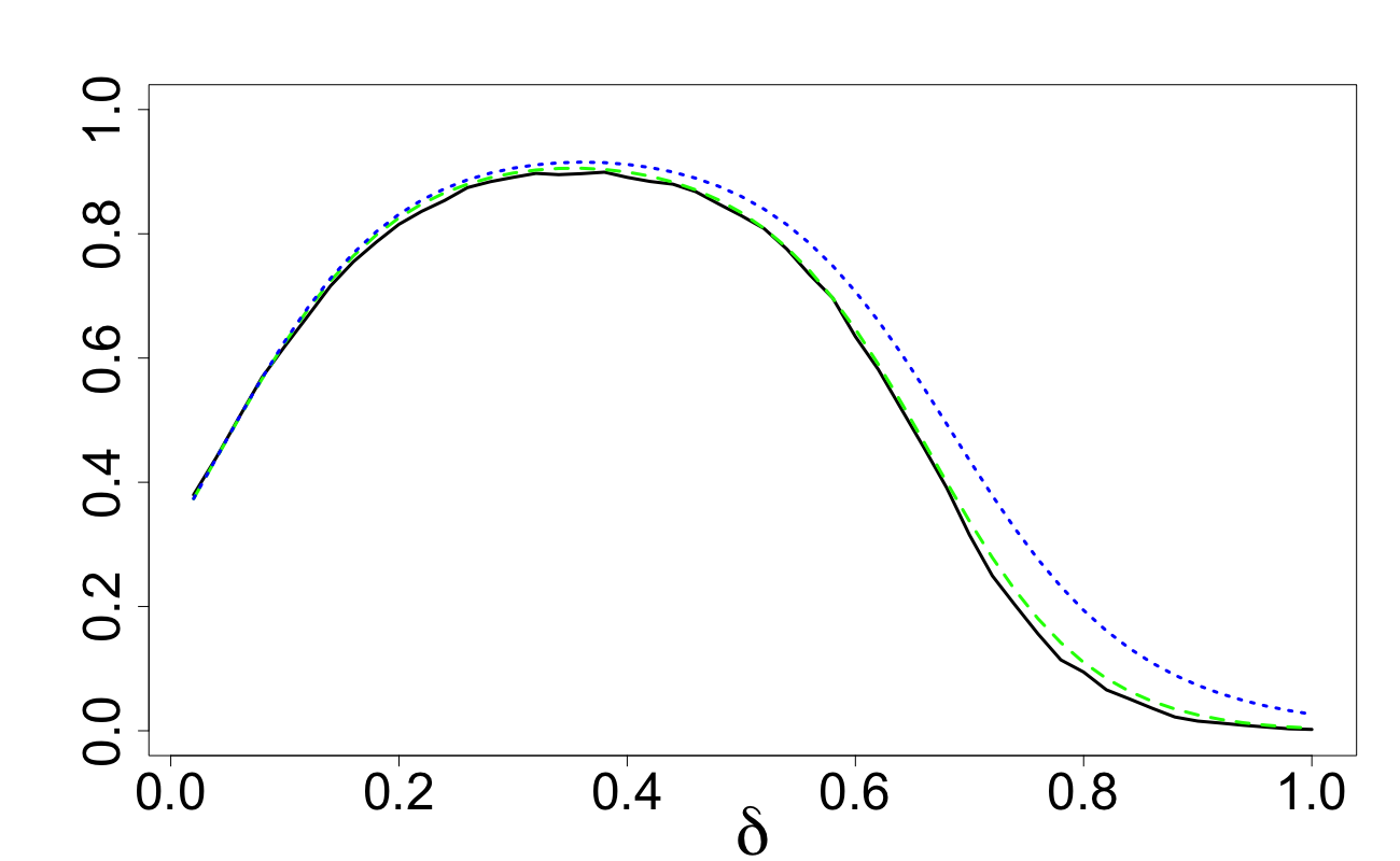
Figure 16: Design 1: $C_{d}(\mathbb{Z}_{n},r)$ and approximations;
$d=20,\alpha=0.1,n=128$.

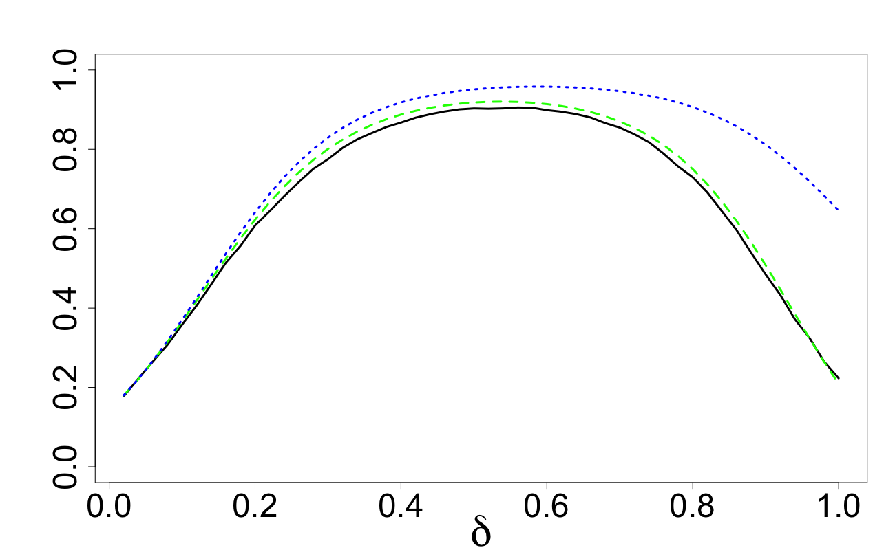
Figure 17: Design 1: $C_{d}(\mathbb{Z}_{n},r)$ and approximations;
$d=20,\alpha=0.5,n=512$.

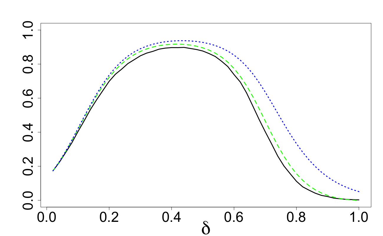
Figure 18: Design 1: $C_{d}(\mathbb{Z}_{n},r)$ and approximations;
$d=20,\alpha=0.1,n=512$.

Figure 19: Design 1: $C_{d}(\mathbb{Z}_{n},r)$ and approximations;
$d=50,\alpha=0.5,n=512$.

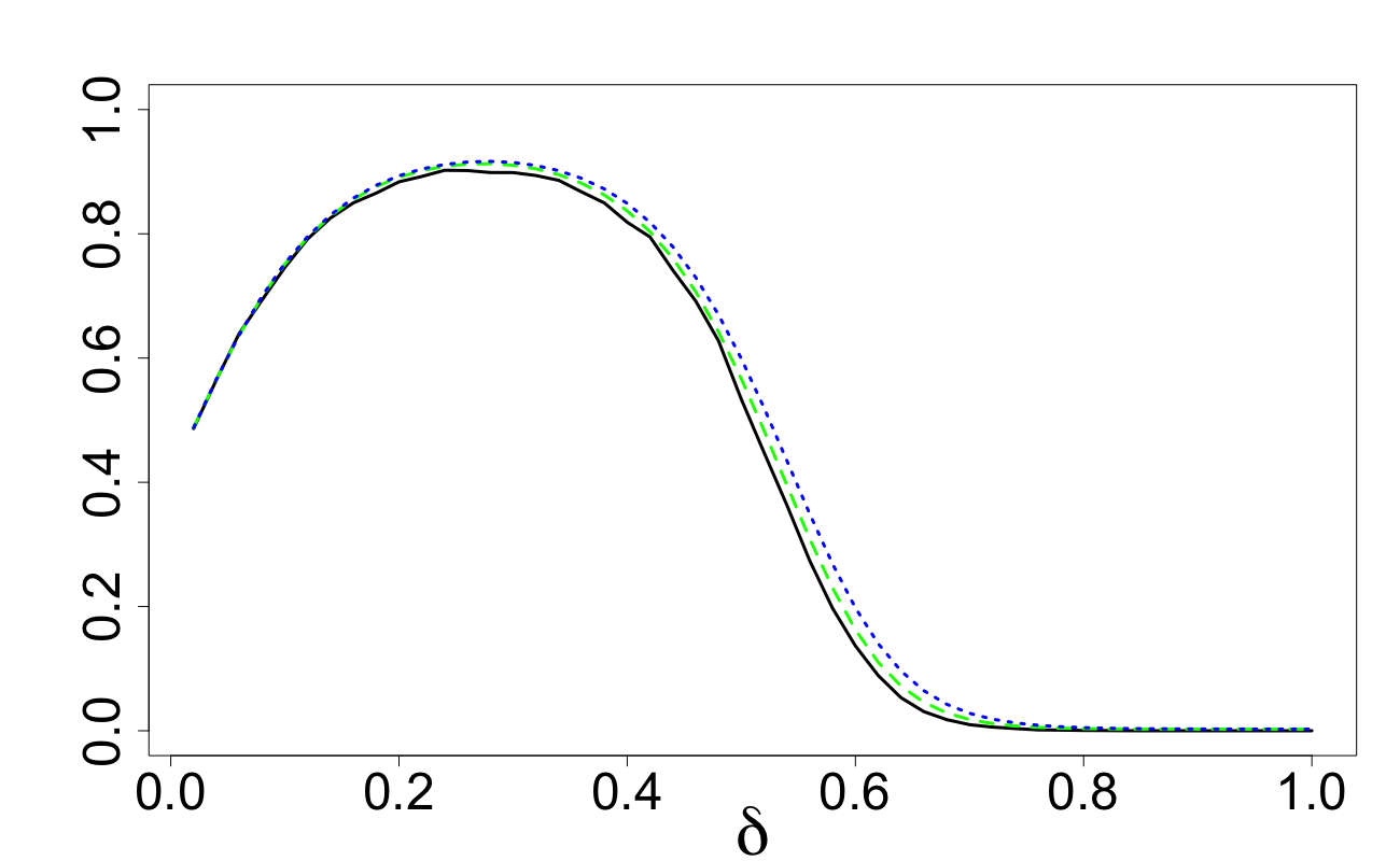
Figure 20: Design 1: $C_{d}(\mathbb{Z}_{n},r)$ and approximations;
$d=50,\alpha=0.1,n=512$.

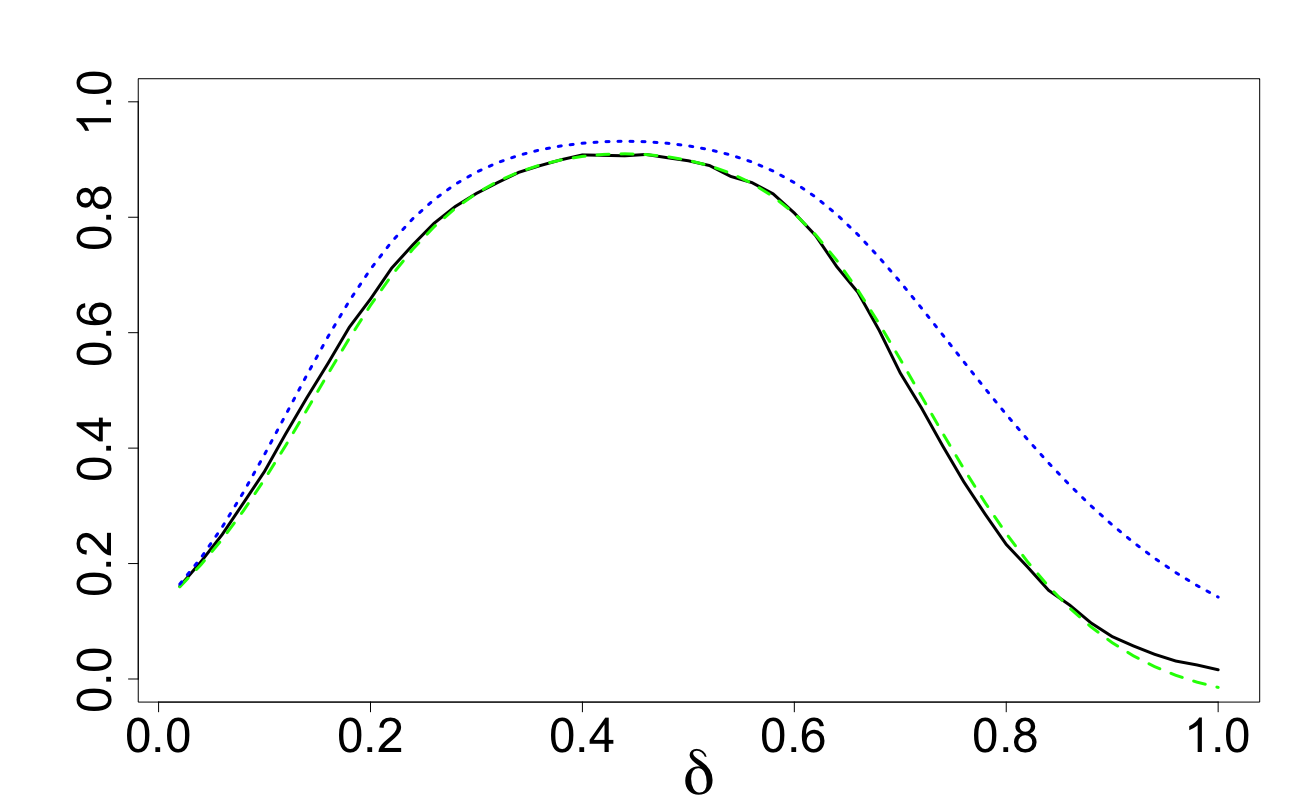
Figure 21: Design 2a: $C_{d}(\mathbb{Z}_{n},r)$ and approximations;
$d=10,\alpha=0,n=128$.

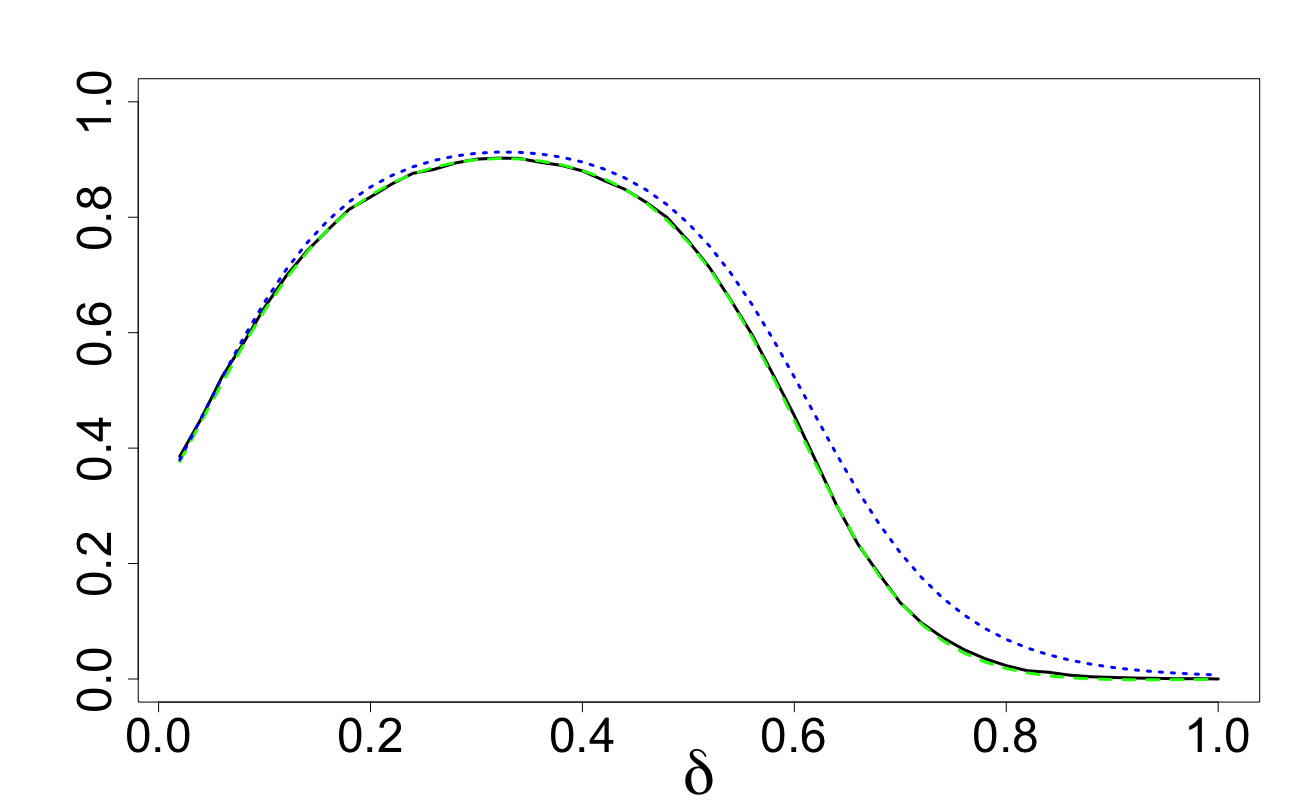
Figure 22: Design 2a: $C_{d}(\mathbb{Z}_{n},r)$ and approximations; $d=20,\alpha=0,n=128$.

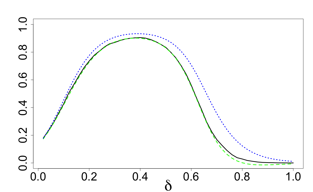
Figure 23: Design 2a: $C_{d}(\mathbb{Z}_{n},r)$ and approximations;
$d=20,\alpha=0,n=512$.

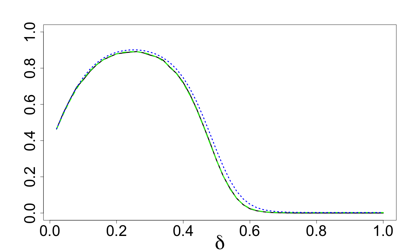
Figure 24: Design 2a: $C_{d}(\mathbb{Z}_{n},r)$ and approximations;
$d=50,\alpha=0,n=512$.

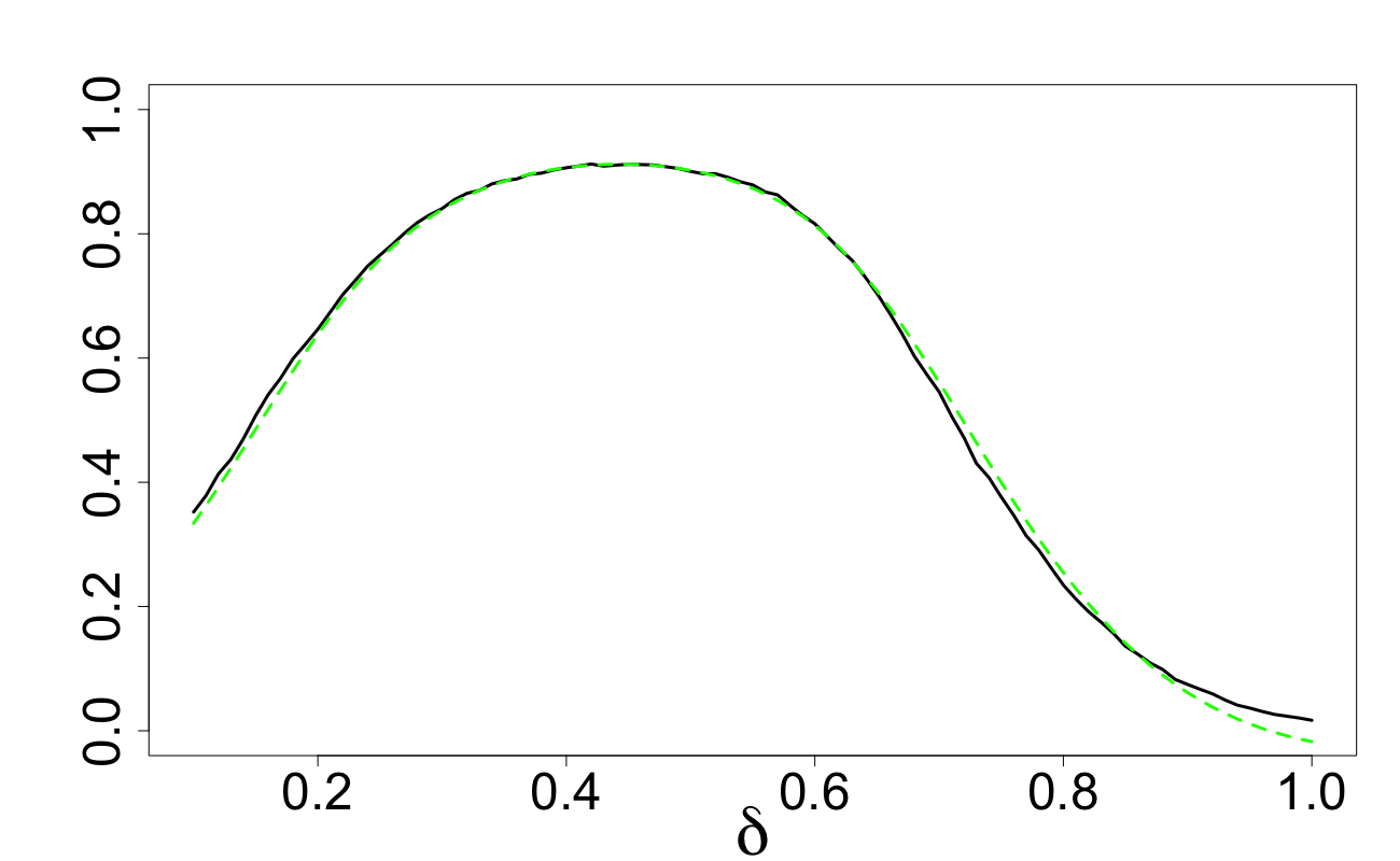
Figure 25: Design 2b: $C_{d}(\mathbb{Z}_{n},r)$ and approxima-
tion (27); $d=10,n=128$.

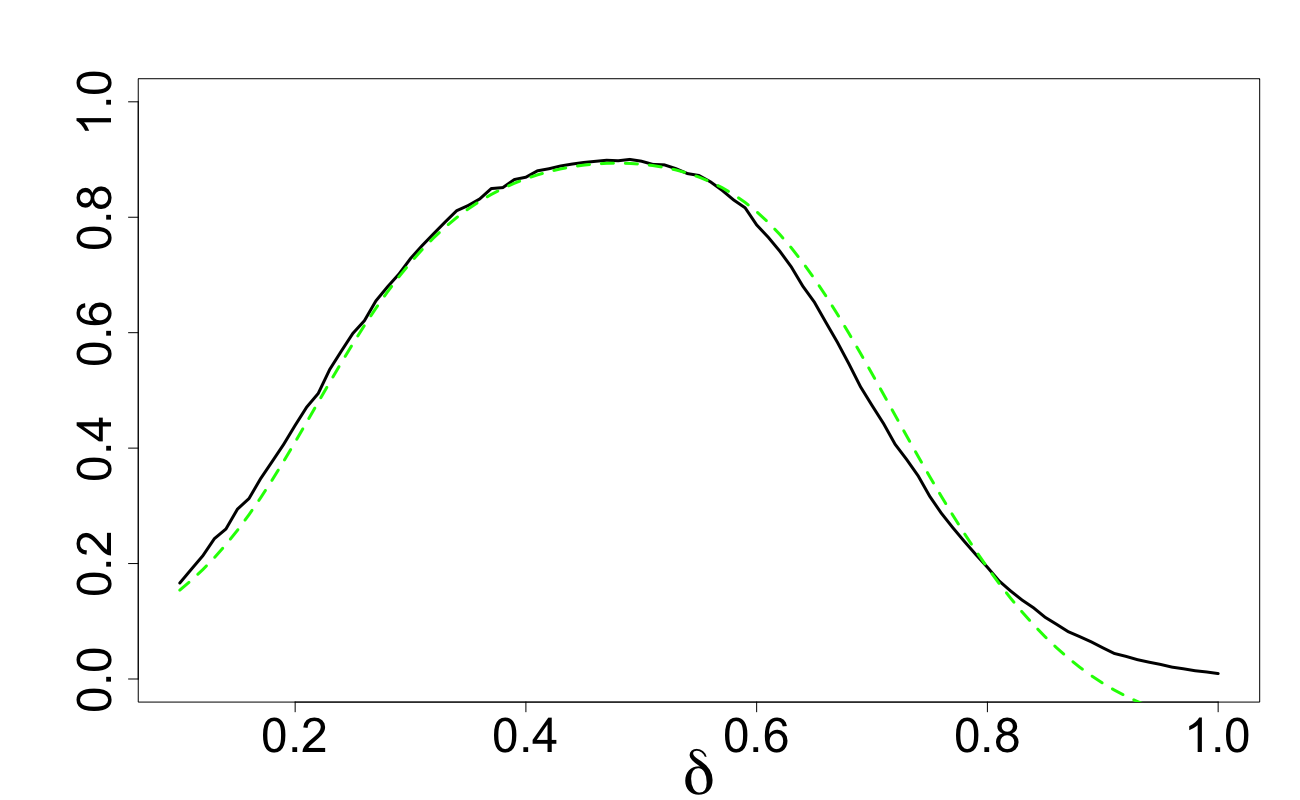
Figure 26: Design 2b: $C_{d}(\mathbb{Z}_{n},r)$ and approximation
(27); $d=10,n=256$.

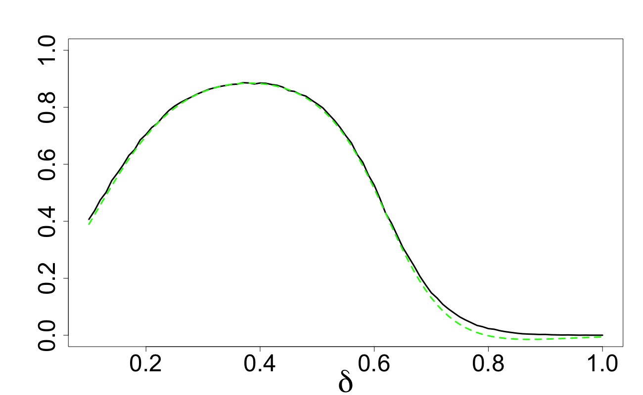
Figure 27: Design 2b: $C_{d}(\mathbb{Z}_{n},r)$ and approxima-
tion (27); $d=20,n=512$.

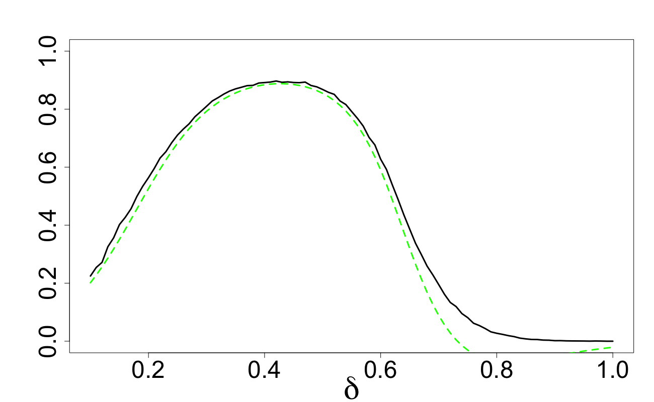
Figure 28: Design 2b: $C_{d}(\mathbb{Z}_{n},r)$ and approximation
(27); $d=20,n=2048$.

6.2 Comparison across $\alpha$

In Table 1, for Design 2a and Design 1 with $\alpha=0.5,1,1.5$ we present the smallest values of $r$ required to achieve the 0.9-coverage on average. For these schemes, the value inside the brackets shows the average value of $\delta$ required to obtain this 0.9-coverage. Design 2b is not used as $d$ is too small (for this design, we must have $n<2^{d}$ and in these cases Design 2b provides better coverings than the other designs considered).

$d=5$
	$n=25$	$n=50$	$n=100$	$n=500$
Design 2a $(\alpha=0)$	1.051 (0.44)	0.885 (0.50)	0.812 (0.50)	0.798 (0.50)
Design 1, $\alpha=0.5$	1.072 (0.68)	0.905 (0.78)	0.770 (0.78)	0.540 (0.80)
Design 1, $\alpha=1$	1.072 (0.78)	0.931 (0.86)	0.798 (0.98)	0.555 (1.00)
Design 1, $\alpha=1.5$	1.091 (0.92)	0.950 (0.96)	0.820 (0.98)	0.589 (1.00)

Table 1: Values of $r$ and $\delta$ (in brackets) to achieve 0.9 coverage for $d=5$.

$d=10$
	$n=500$	$n=1000$	$n=5000$	$n=10000$
Design 2a $(\alpha=0)$	1.228 (0.50)	1.135 (0.50)	1.073 (0.50)	1.071 (0.50)
Design 1, $\alpha=0.5$	1.271 (0.69)	1.165 (0.73)	0.954 (0.76)	0.886 (0.78)
Design 1, $\alpha=1$	1.297 (0.87)	1.194 (0.90)	0.992 (0.93)	0.917 (0.95)
Design 1, $\alpha=1.5$	1.320 (1.00)	1.220 (1.00)	1.032 (1.00)	0.953 (1.00)

Table 2: Values of $r$ and $\delta$ (in brackets) to achieve 0.9 coverage for $d=10$.

From Tables 1 and 2 we can make the following conclusions:

• For small $n$ ($n<2^{d}$ or $n\simeq 2^{d}$), Design 2a provides a more efficient covering than other three other schemes and hence smaller values of $\alpha$ are better.

• For $n>2^{d}$, Design 2a begins to become impractical since a large proportion of points duplicate. This is reflected in Table 1 by comparing $n=100$ and $n=500$ for Design 2a; there is only a small reduction in $r$ despite a large increase in $n$. Moreover, for values of $n>>2^{d}$, Design 2a provides a very inefficient covering.

• For $n>>2^{d}$, from looking at Design 1 with $\alpha=0.5$ and $n=500$, it would appear beneficial to choose $\alpha\in(0,1)$ rather than $\alpha>1$ or $\alpha=0$.

Using approximations (18) and (24), in Figures 30–30 we depict $C_{d}(\mathbb{Z}_{n},r)$ across $\delta$ for different choices of $\alpha$. In Figures 30–30, the red line, green line, blue line and cyan line depict approximation (24) ($\alpha=0$) and approximation (18) with $\alpha=0.5$, $\alpha=1$ and $\alpha=1.5$ respectively. These figures demonstrate the clear benefit of choosing a smaller $\alpha$, at least for these values of $n$ and $d$.

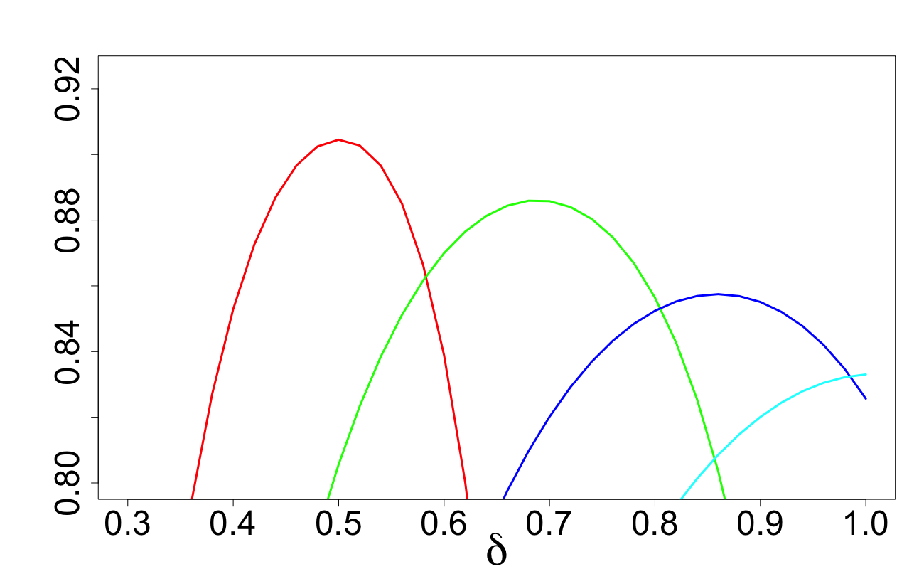
Figure 29: $d=10$, $n=512$, $r=1.228$

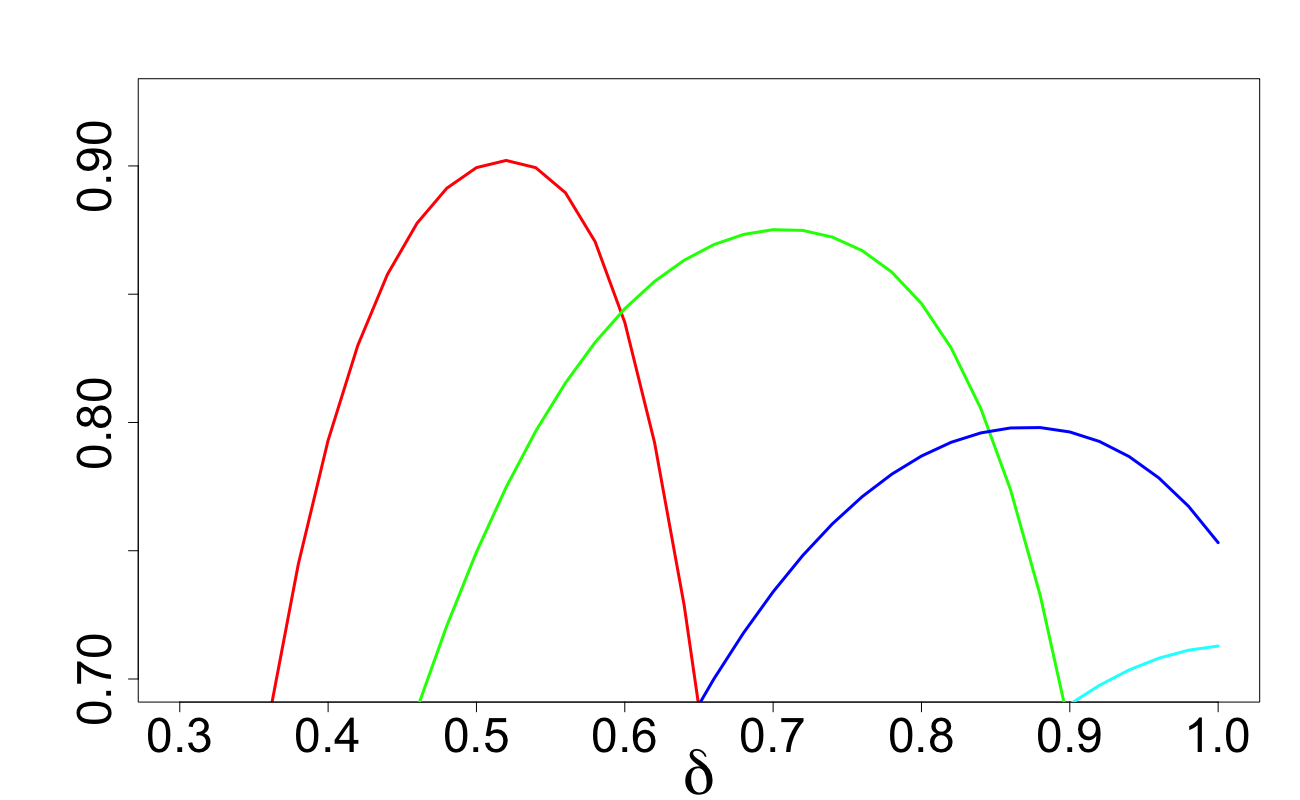
Figure 30: $d=10$, $n=1024$, $r=1.13$

7 Quantization in a cube

7.1 Quantization error and its relation to weak covering

In this section, we will study the following characteristic of a design $\mathbb{Z}_{n}$.

Quantization error. Let $U=(u_{1},\ldots,u_{d})$ be uniform random vector on $[-1,1]^{d}$. The mean squared quantization error for a design $\mathbb{Z}_{n}=\{Z_{1},\ldots,Z_{n}\}\subset\mathbb{R}^{d}$ is defined by

$$\theta(\mathbb{Z}_{n})=\mathbb{E}_{U}\varrho^{2}(U,\mathbb{Z}_{n})\,,\;\;{\rm where}\;\;\varrho(U,\mathbb{Z}_{n})=\min_{Z_{i}\in\mathbb{Z}_{n}}\|U-Z_{i}\|\,.$$ (29)

If the design $\mathbb{Z}_{n}$ is randomized then we consider the expected value $\mathbb{E}_{\mathbb{Z}_{n}}\theta(\mathbb{Z}_{n})$ of $\theta(\mathbb{Z}_{n})$ as the main characteristic without stressing this.

The mean squared quantization error $\theta(\mathbb{Z}_{n})$ is related to our main quantity $C_{d}(\mathbb{Z}_{n},r)$ defined in (1): indeed, $C_{d}(\mathbb{Z}_{n},r)$, as a function of $r\geq 0$, is the c.d.f. of the r.v. $\varrho(U,\mathbb{Z}_{n})$ while $\theta(\mathbb{Z}_{n})$ is the second moment of the distribution with this c.d.f.:

$$\theta(\mathbb{Z}_{n})=\int_{r\geq 0}r^{2}dC_{d}(\mathbb{Z}_{n},r)\,.$$ (30)

This relation will allow us to use the approximations derived above for $C_{d}(\mathbb{Z}_{n},r)$ in order to construct approximations for the quantization error $\theta(\mathbb{Z}_{n})$.

7.2 Quantization error for Design 1

Using approximation (18) for the quantity $C_{d}(\mathbb{Z}_{n},r)$, we obtain

$$\frac{d}{dr}(C_{d}(\mathbb{Z}_{n},r))\cong f_{\alpha,\delta}(r):=\frac{n\cdot r}{\delta}\int_{-\infty}^{\infty}\varphi(s)\varphi(c_{s})\psi_{2,\alpha}(s)\times$$

$$\times\left[\frac{\sqrt{2\alpha+1}}{\sqrt{s^{\prime}+k}}+c_{d,\alpha}\frac{\alpha\left(s^{\prime}+\frac{d\delta^{2}(2\alpha-1)}{3(2\alpha+5)(2\alpha+1)}\right)}{(2\alpha+3)\left(s^{\prime}+k\right)^{2}}\left\{{\delta(c_{s}^{3}-c_{s})}-\frac{\sqrt{2\alpha+1}(r^{2}-\frac{d\delta^{2}}{2\alpha+1}-s^{\prime})}{\sqrt{s^{\prime}+k}}\right\}\right]ds\,.$$ (31)

By then using relation (30) we obtain the following approximation for the mean squared quantization error with Design 1:

$$\theta(\mathbb{Z}_{n})\cong\int_{0}^{\infty}r^{2}f_{\alpha,\delta}(r)dr\,.$$ (32)

By taking $\alpha=1$ in (7.2) we obtain:

$$f_{1,\delta}(r)\!\!\! := \!\!\frac{n\cdot r}{\delta}\int_{-\infty}^{\infty}\varphi(s)\varphi(c_{s})\psi_{2,1}(s)\!\left[\frac{\sqrt{3}}{\sqrt{s^{\prime}+k}}+c_{d,1}\frac{\left(s^{\prime}+\frac{d\delta^{2}}{63}\right)}{5\left(s^{\prime}+k\right)^{2}}\left\{{\delta(c_{s}^{3}-c_{s})}-\frac{\sqrt{3}(r^{2}-\frac{d\delta^{2}}{3}-s^{\prime})}{\sqrt{s^{\prime}+k}}\right\}\right]ds\,.$$

with $\psi_{2,1}$ defined in (19). The resulting approximation

$$\theta(\mathbb{Z}_{n})\cong\int_{0}^{\infty}r^{2}f_{1,\delta}(r)dr\,.$$

coincides with (us, , formula 31).

7.3 Quantization error for Design 2a

Using approximation (24) for the quantity $C_{d}(\mathbb{Z}_{n},r)$, we have:

$$\frac{d}{dr}(C_{d}(\mathbb{Z}_{n},r))\cong f_{0,\delta;n}(r):=\;\;\;\;\;\;\;\;\;\;\;\;\;\;\;\;\;\;\;\;\;\;\;\;\;\;\;\;\;\;\;\;\;\;\;\;\;\;\;\;\;\;\;\;\;\;\;\;\;\;\;\;\;\;\;\;\;\;\;\;\;\;\;\;\;\;\;\;\;\;\;\;\;\;\;\;\;\;\;\;\;\;\;\;\;\;\;\;$$

$$\frac{n\cdot r}{\delta}\int_{-\infty}^{\infty}\frac{\varphi(s)\varphi(c_{s})\psi_{4,n}(s)}{\sqrt{s^{\prime}}}\left[1+\left(1+\frac{3}{d}\right)\frac{(2(s^{\prime}-d/3)/\sqrt{5}+d/5)(6c_{s}^{2}-c_{s}^{4}-3)}{12(s^{\prime})^{2}}\right]ds\,,$$ (33)

where $\psi_{4,n}(\cdot)$ is defined in (25). From (30) we then obtain the following approximation for the mean squared quantization error with Design 2a:

$$\theta(\mathbb{Z}_{n})\cong\int_{0}^{\infty}r^{2}f_{0,\delta;n}(r)dr\,.$$ (34)

7.4 Quantization error for Design 2b

Similarly to (34), for Design 2b, we use the approximation

$$\theta(\mathbb{Z}_{n})\cong\int_{0}^{\infty}r^{2}f_{0,\delta;m}(r)dr\,.$$ (35)

where $f_{0,\delta,m}(r)$ is defined by (33) and $m=m_{n,d}$ is defined in (28).

7.5 Accuracy of approximations for quantization error and the $\delta$-effect

In this section, we assess the accuracy of approximations (32), (34) and (35). Using a black line we depict $\mathbb{E}_{\mathbb{Z}_{n}}\theta(\mathbb{Z}_{n})$ obtained via Monte Carlo simulations. Depending on the value of $\alpha$, in Figures 32–36 approximation (32) or (34) is shown using a red line. In Figures 42–44, approximation (35) is depicted with a red line. From the figures below we can see that all approximations are generally very accurate. Approximation (34) is much more accurate than approximation (32) across all choices of $\delta$ and $n$ and this can be explained by the additional term taken in the general expansion; see Section 4.2. This high accuracy is also seen with approximation (35). The accuracy of approximation (32) seems to worsen for large $\delta$, $n$ and $d$ not too large like $d=20$, see Figures 34–34. For $d=50$, all approximations are extremely accurate for all choices of $\delta$ and $n$. Figures 32–36 very clearly demonstrate the $\delta$-effect implying that a sensible choice of $\delta$ is crucial for good quantization.

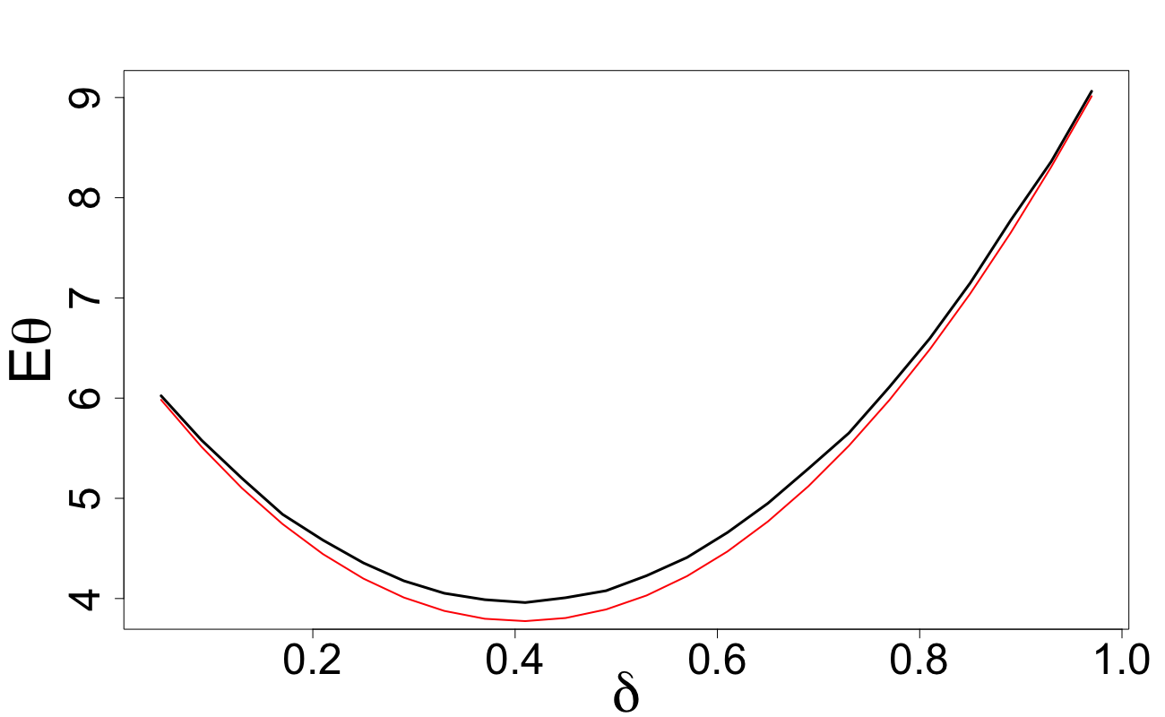
Figure 31: $\mathbb{E}\theta(\mathbb{Z}_{n})$ and approximation (32)$:d=20$,
$\alpha=1$, $n=500$

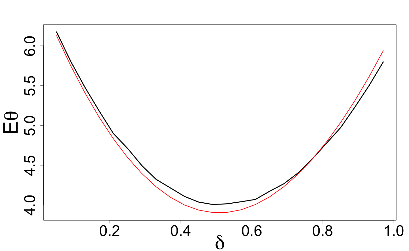
Figure 32: $\mathbb{E}\theta(\mathbb{Z}_{n})$ and approximation (32)$:d=20$,
$\alpha=0.5$, $n=500$

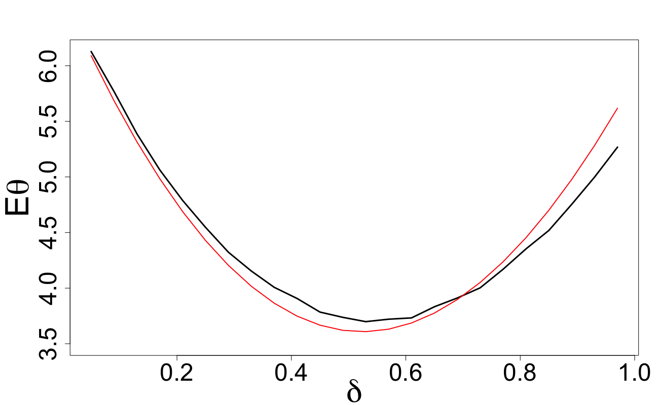
Figure 33: $\mathbb{E}\theta(\mathbb{Z}_{n})$ and approximation (32): $d=20$,
$\alpha=0.5$, $n=1000$

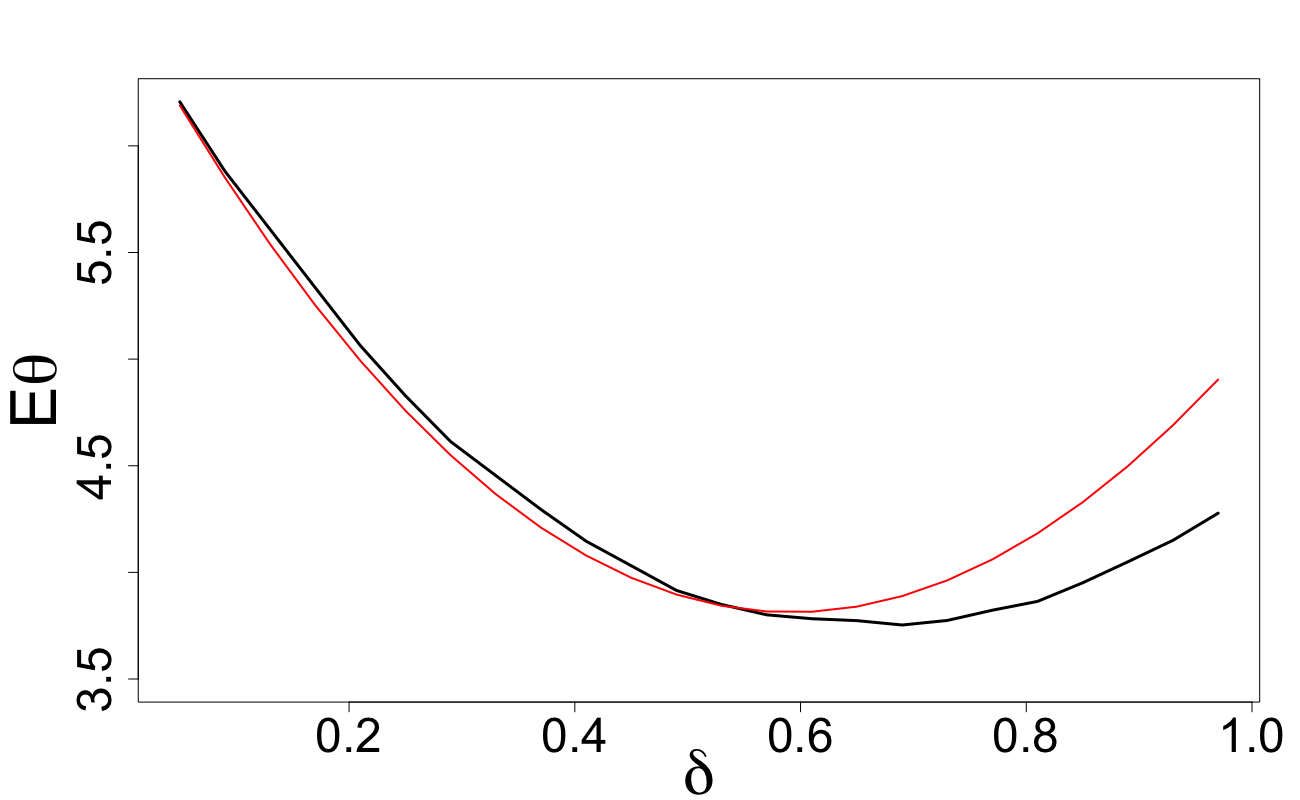
Figure 34: $\mathbb{E}\theta(\mathbb{Z}_{n})$ and approximation (32): $d=20$,
$\alpha=1$, $n=1000$

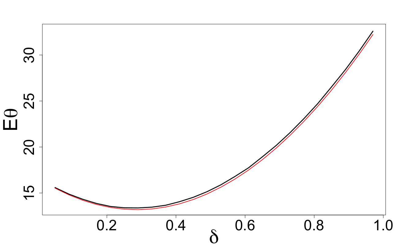
Figure 35: $\mathbb{E}\theta(\mathbb{Z}_{n})$ and approximation (32): $d=50$,
$\alpha=0.1$, $n=1000$

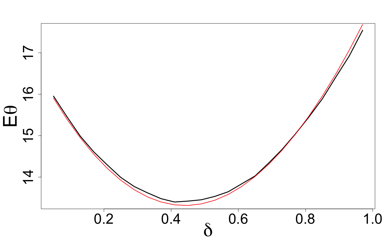
Figure 36: $\mathbb{E}\theta(\mathbb{Z}_{n})$ and approximation (32): $d=50$,
$\alpha=1$, $n=1000$

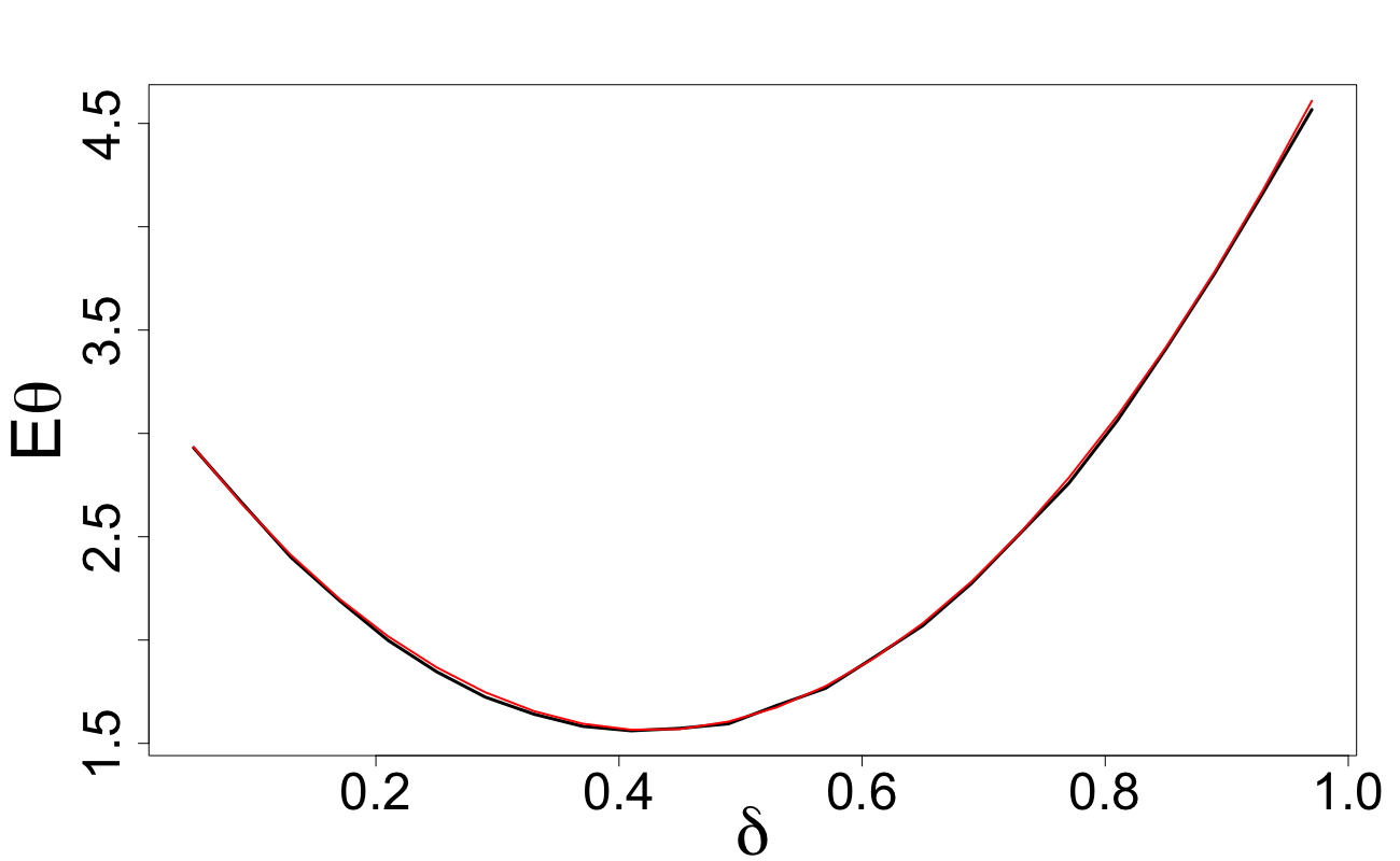
Figure 37: $\mathbb{E}\theta(\mathbb{Z}_{n})$ and approximation (34): $d=10$,
$\alpha=0$, $n=100$

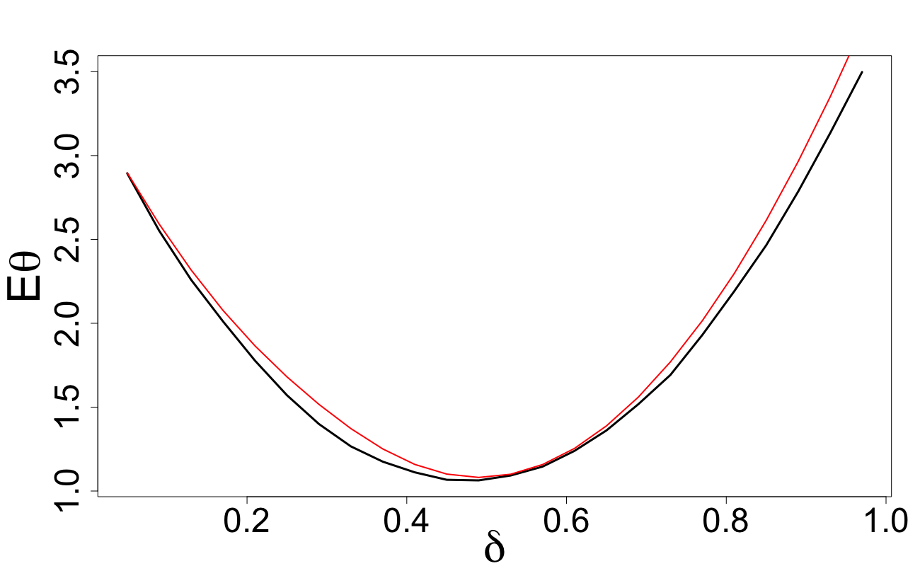
Figure 38: $\mathbb{E}\theta(\mathbb{Z}_{n})$ and approximation (34): $d=10$,
$\alpha=0$, $n=500$

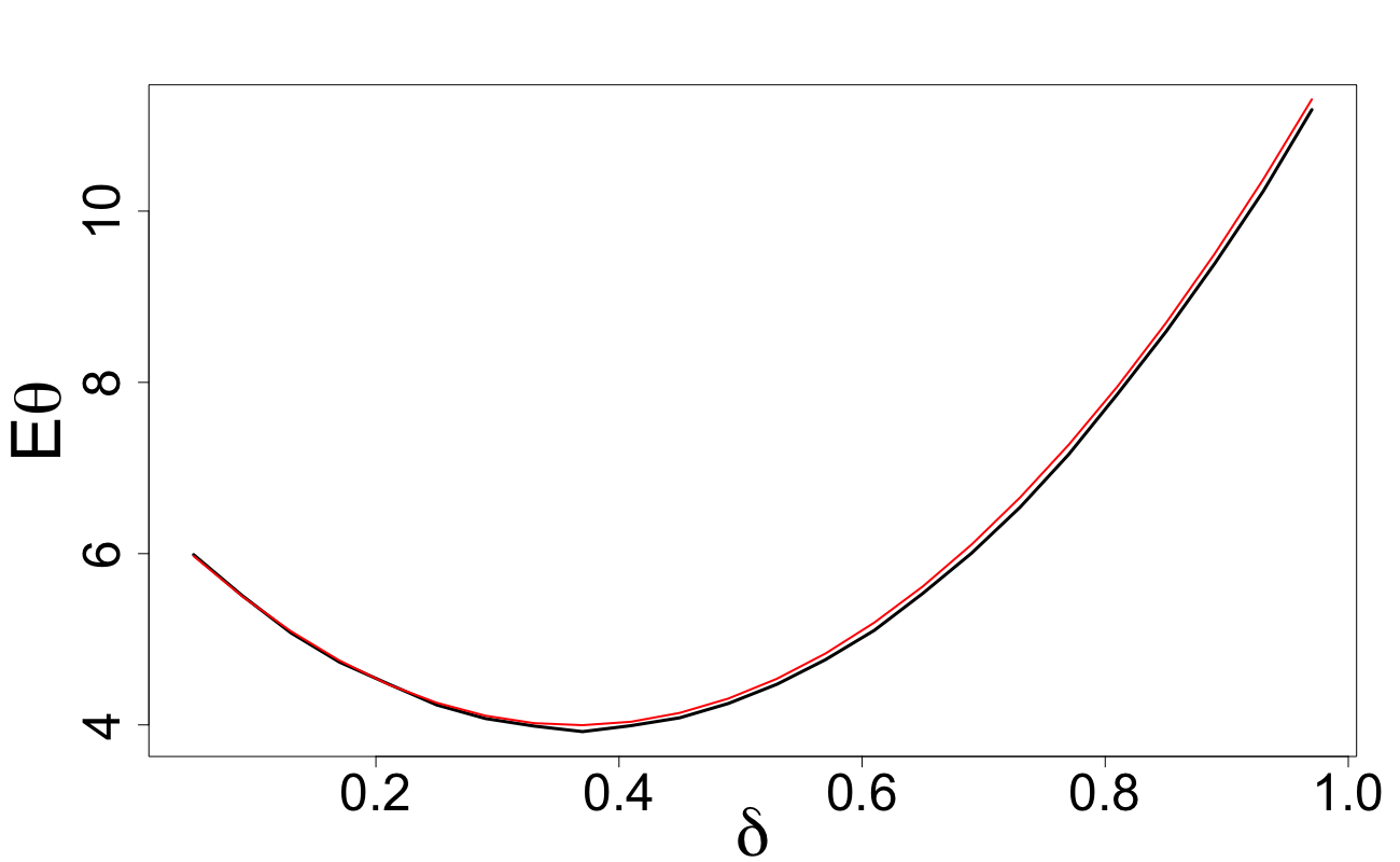
Figure 39: $\mathbb{E}\theta(\mathbb{Z}_{n})$ and approximation (34): $d=20$,
$\alpha=0$, $n=500$

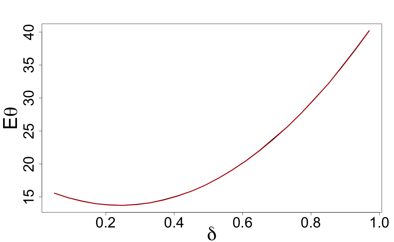
Figure 40: $\mathbb{E}\theta(\mathbb{Z}_{n})$ and approximation (34): $d=50$,
$\alpha=0$, $n=500$

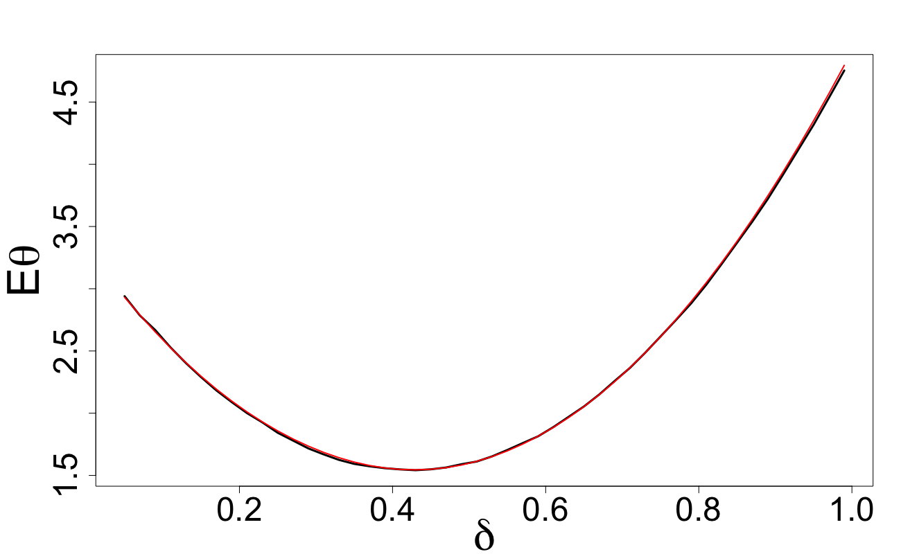
Figure 41: $\mathbb{E}\theta(\mathbb{Z}_{n})$ and approximation (35): $d=10$,
$n=100$

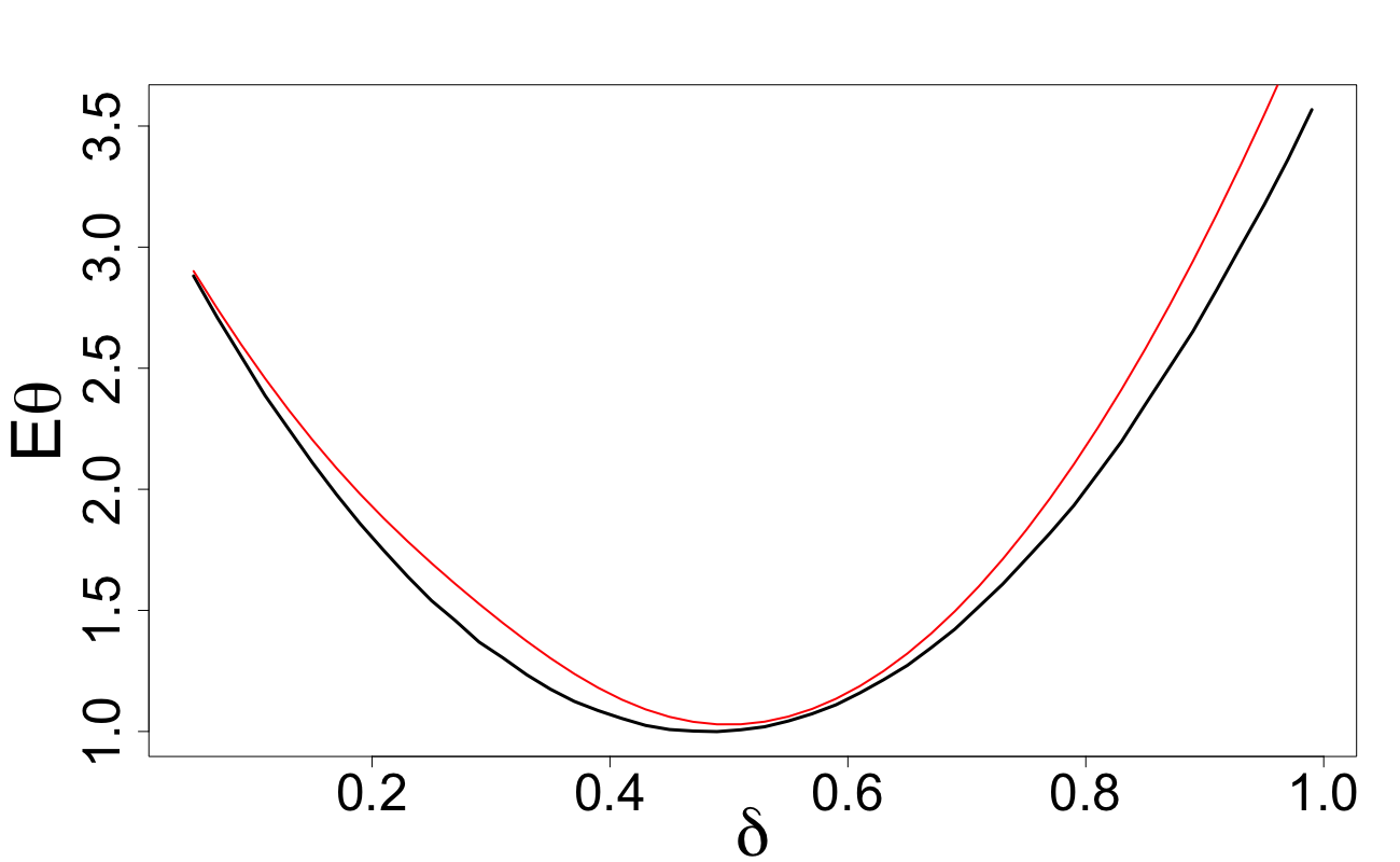
Figure 42: $\mathbb{E}\theta(\mathbb{Z}_{n})$ and approximation (35): $d=10$,
$n=500$

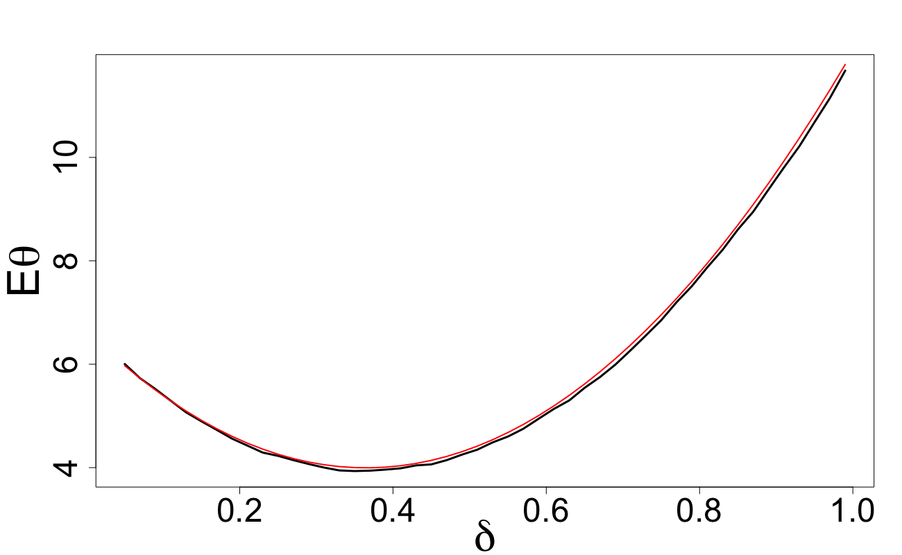
Figure 43: $\mathbb{E}\theta(\mathbb{Z}_{n})$ and approximation (35): $d=20$,
$n=500$

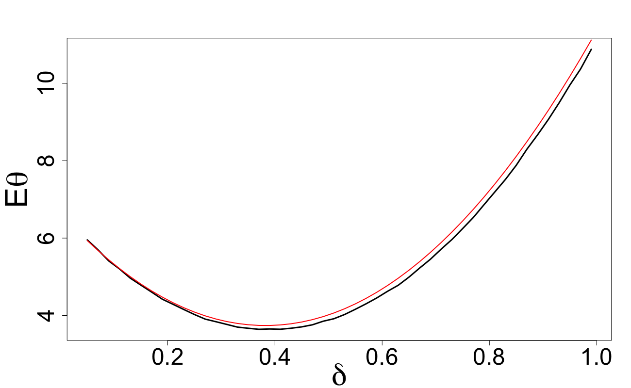
Figure 44: $\mathbb{E}\theta(\mathbb{Z}_{n})$ and approximation (35): $d=20$,
$n=1000$

8 Comparative numerical studies of covering properties for several designs

Let us extend the range of designs considered above by additing the following two designs.

Design 3. $Z_{1},\ldots,Z_{n}$ are taken from a low-discrepancy Sobol’s sequence on the cube $[-\delta,\delta]^{d}$.

Design 4. $Z_{1},\ldots,Z_{n}$ are taken from the minimum-aberration $2^{d-k}$ fractional factorial design on the vertices of the cube $[-\delta,\delta]^{d}$.

Unlike Designs 1, 2a, 2b and 3, Design 4 is non-adaptive and defined only for a particular $n$ of the form $n=2^{d-k}$ with some $k\geq 0$. We have included this design into the list of all designs as ”the golden standard”. In view of the numerical study in us and theoretical arguments in us1 , Design 4 with $k=1$ and optimal $\delta$ provides the best quantization we were able to find; moreover, we have conjectured in us1 that Design 4 with $k=1$ and optimal $\delta$ provides minimal normalized mean squared quantization error for all designs with $n\leq 2^{d}$. We repeat, Design 4 is defined for one particular value of $n$ only.

8.1 Covering comparisons

In Tables 3–4, we present results of Monte Carlo simulations where we have computed the smallest values of $r$ required to achieve the 0.9-coverage on average (on average, for Designs 1, 2a, 2b). The value inside the brackets shows the value of $\delta$ required to obtain the 0.9-coverage.

$d=10$
	$n=64$	$n=128$	$n=512$	$n=1024$
Design 1, $\alpha=0.5$	1.629 (0.58)	1.505 (0.65)	1.270 (0.72)	1.165 (0.75)
Design 1, $\alpha=1.5$	1.635 (0.80)	1.525 (0.88)	1.310 (1.00)	1.210 (1.00)
Design 2a	1.610 (0.38)	1.490 (0.46)	1.228 (0.50)	1.132 (0.50)
Design 2b	1.609 (0.41)	1.475 (0.43)	1.178 (0.49)	1.075 (0.50)
Design 3	1.595 (0.72)	1.485 (0.80)	1.280 (0.85)	1.170 (0.88)
Design 3, $\delta=1$	1.678 (1.00)	1.534 (1.00)	1.305 (1.00)	1.187 (1.00)
Design 4	1.530 (0.44)	1.395 (0.48)	1.115 (0.50)	1.075 (0.50)

Table 3: Values of $r$ and $\delta$ (in brackets) to achieve 0.9 coverage for $d=10$.

$d=20$
	$n=64$	$n=128$	$n=512$	$n=1024$
Design 1, $\alpha=0.5$	2.540 (0.44)	2.455 (0.48)	2.285 (0.55)	2.220 (0.60)
Design 1, $\alpha=1.5$	2.545 (0.60)	2.460 (0.65)	2.290 (0.76)	2.215 (0.84)
Design 2a	2.538 (0.28)	2.445 (0.30)	2.270 (0.36)	2.180 (0.42)
Design 2b	2.538 (0.29)	2.445 (0.30)	2.253 (0.37)	2.173 (0.42)
Design 3	2.520 (0.50)	2.445 (0.60)	2.285 (0.68)	2.196 (0.72)
Design 3, $\delta=1$	2.750 (1.00)	2.656 (1.00)	2.435 (1.00)	2.325 (1.00)
Design 4	2.490 (0.32)	2.410 (0.35)	2.220 (0.40)	2.125 (0.44)

Table 4: Values of $r$ and $\delta$ (in brackets) to achieve 0.9 coverage for $d=20$.

From Tables 3–4 we draw the following conclusions:

• Designs 2a and especially 2b provide very high quality coverage (on average) whilst being online procedures (that is, nested designs);

• Design 2b has significant benefits over Design 2a for values of $n$ close to $2^{d}$;

• properly $\delta$-tuned deterministic non-nested Design 4 provides superior covering;

• coverage properties of $\delta$-tuned low-discrepancy sequences are much better than of the original low-discrepancy sequences;

• coverage of an unadjusted low-discrepancy sequence is poor.

In Figures 46–46, after fixing $n$ and $\delta$, we plot $C_{d}(\mathbb{Z}_{n},r)$ as a function of $r$ for the following designs: Design 1 with $\alpha=1$ (red line), Design 2a (blue line), Design 2b (green line) and Design 3 with $\delta=1$ (black line). For Design 1 with $\alpha=1$, Design 2a and Design 2b, we have used approximations (19), (25) and (27) respectively to depict $C_{d}(\mathbb{Z}_{n},r)$ whereas for Design 3, we have used Monte Carlo simulations. For the first three designs, depending of the choice of $n$, the value of $\delta$ has been fixed based on the optimal value for quantization; these are the values inside the brackets in Tables 5–6.

From Figure 46, we see that Design 2b is superior and uniformly dominates all other designs for this choice of $d$ and $n$ (at least when the level of coverage is greater than 1/2). In Figure 46, since $n<<2^{d}$, the values of $C_{d}(\mathbb{Z}_{n},r)$ for Designs 2a and 2b practically coincide and the green line hides under the blue. In both figures we see that Design 3 with an unadjusted $\delta$ provides a very inefficient covering.

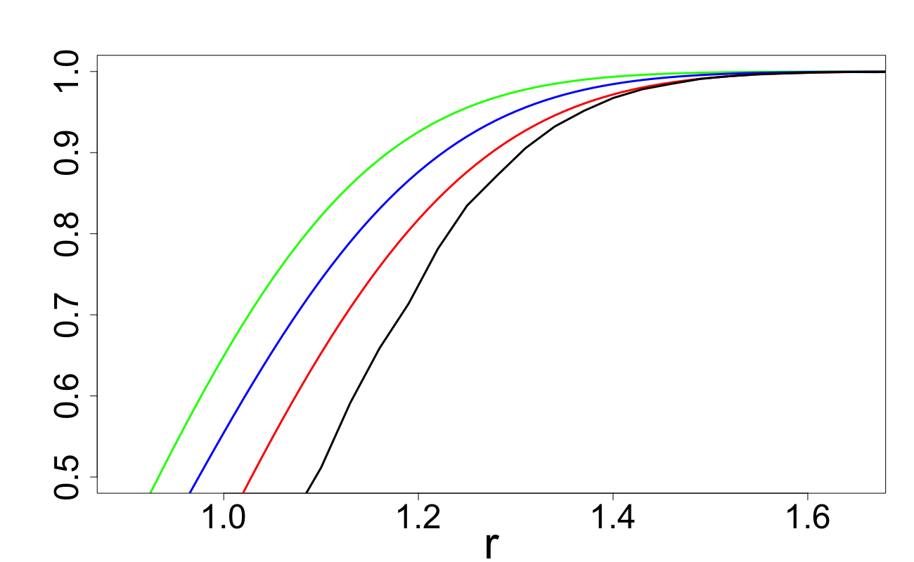
Figure 45: $C_{d}(\mathbb{Z}_{n},r)$ as a function of $r$ for several
designs: $d=10$, $n=512$

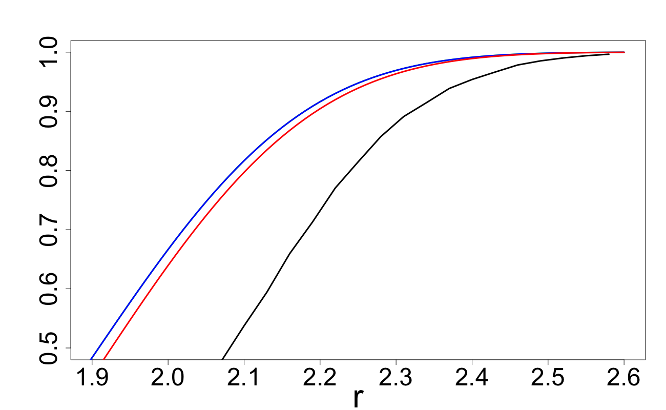
Figure 46: $C_{d}(\mathbb{Z}_{n},r)$ as a function of $r$ for several
designs: $d=20$, $n=1024$

8.2 Quantization comparisons

As follows from results of (niederreiter1992random, , Ch.6), for efficient covering schemes the order of convergence of the covering radius to 0 as $n\to\infty$ is $n^{-1/d}$. Therefore, for the mean squared distance (which is the quantization error) we should expect the order $n^{-2/d}$ as $n\to\infty$. Therefore, for sake of comparison of quantization errors $\theta_{n}$ across $n$ we renormalize this error from $\mathbb{E}\theta_{n}$ to $n^{2/d}\mathbb{E}\theta_{n}$.

In Figure 48–6, we present the minimum value of $n^{2/d}\mathbb{E}\theta_{n}$ for a selection of designs. In these tables, the value within the brackets corresponds to the value of $\delta$ where the minimum of $n^{2/d}\mathbb{E}\theta_{n}$ was obtained.

$d=10$
	$n=64$	$n=128$	$n=512$	$n=1024$
Design 1, $\alpha=0.5$	4.072 (0.56)	4.013 (0.60)	3.839 (0.68)	3.770 (0.69)
Design 1, $\alpha=1$	4.153 (0.68)	4.105 (0.72)	3.992 (0.80)	3.925 (0.84)
Design 1, $\alpha=1.5$	4.164 (0.80)	4.137 (0.86)	4.069 (0.96)	4.026 (0.98)
Design 2a	3.971 (0.38)	3.866 (0.44)	3.670 (0.48)	3.704 (0.50)
Design 2b	3.955 (0.40)	3.798 (0.44)	3.453 (0.48)	3.348 (0.50)
Design 3	3.998 (0.68)	3.973 (0.76)	3.936 (0.80)	3.834 (0.82)
Design 3, $\delta=1$	4.569 (1.00)	4.425 (1.00)	4.239 (1.00)	4.094 (1.00)
Design 4	3.663 (0.40)	3.548 (0.44)	3.221 (0.48)	3.348 (0.50)

Table 5: Minimum value of $n^{2/d}\mathbb{E}\theta_{n}$ and $\delta$ (in brackets) across selected designs; $d=10$.

$d=20$
	$n=64$	$n=128$	$n=512$	$n=1024$
Design 1, $\alpha=0.5$	7.541 (0.40)	7.515 (0.44)	7.457 (0.52)	7.421 (0.54)
Design 1, $\alpha=1$	7.552 (0.52)	7.563 (0.56)	7.528 (0.64)	7.484 (0.68)
Design 1, $\alpha=1.5$	7.561 (0.60)	7.571 (0.64)	7.556 (0.74)	7.527 (0.78)
Design 2a	7.488 (0.30)	7.461 (0.33)	7.346 (0.35)	7.248 (0.39)
Design 2b	7.487 (0.29)	7.458 (0.34)	7.345 (0.36)	7.234 (0.40)
Design 3	7.445 (0.48)	7.464 (0.56)	7.487 (0.64)	7.453 (0.66)
Design 3, $\delta=1$	9.089 (1.00)	9.133 (1.00)	8.871 (1.00)	8.681 (1.00)
Design 4	7.298 (0.32)	7.270 (0.33)	7.133 (0.36)	7.016 (0.40)

Table 6: Minimum value of $n^{2/d}\mathbb{E}\theta_{n}$ and $\delta$ (in brackets) across selected designs; $d=20$.

In Figure 48, we depict the c.d.f.’s for the distance $\varrho(X,\mathbb{Z}_{n})$ for Design 2a with $\delta=0.5$ (in red) and Design 3 with $\delta=0.8$ (in black). We can see that for $d=10$ and $n=512$, Design 2a stochastically dominates Design 3. The style of Figure 48 is the same as figure Figure 48, however we set $n=1024$ and Design 2a is replaced with Design 2b with $\delta=0.5$ (we also set $\delta=0.82$ for Design 3). Here we see a very clear stochastic dominance of the Design 2b over Design 4. All findings are consistent with Tables 5 and 6. In Figures 48 and 48, values of the parameter $\delta$ for all designs are chosen as numerically optimal, in accordance with Table 5.

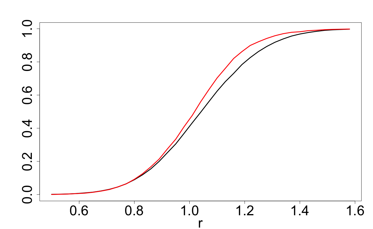
Figure 47: $d=10,n=512$: Design 2a with
$\delta=0.5$ stochastically dominates Design 3
with $\delta=0.8$.

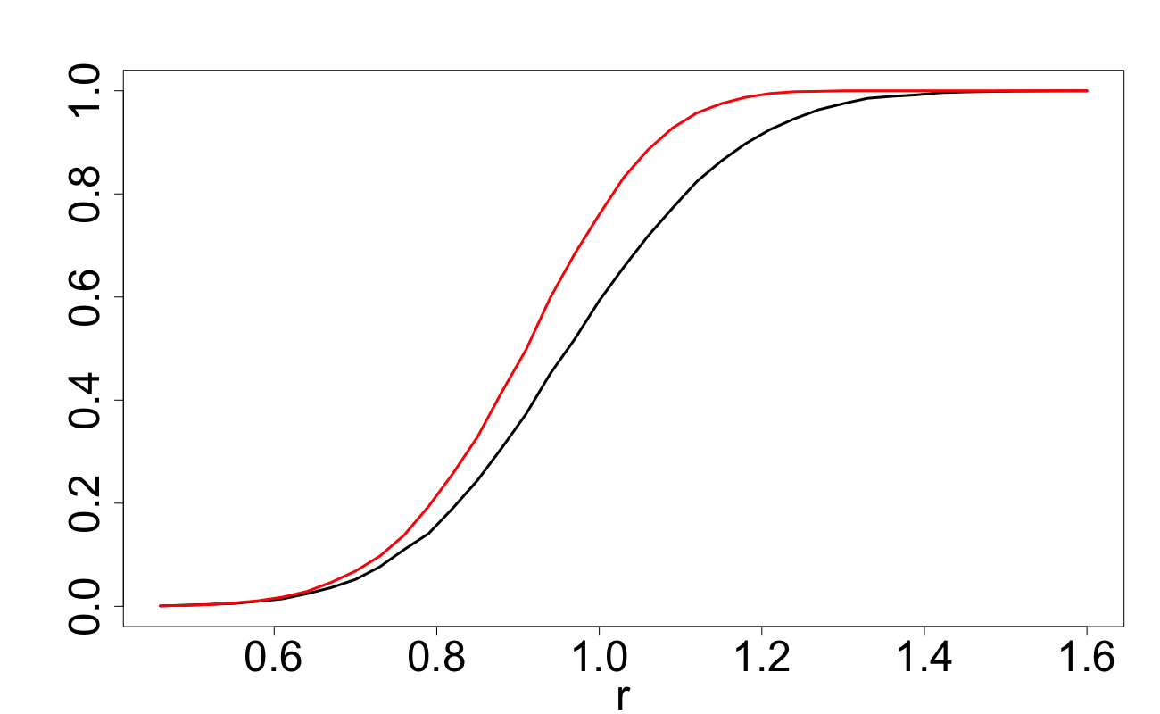
Figure 48: $d=10,n=1024$: Design 2b with
$\delta=0.5$ stochastically dominates Design 3
with $\delta=0.82$.

We make the following conclusions from analyzing results of this section:

• Designs 2a and 2b provide very good quantization per point. As expected, Design 2b is superior over Design 2a when $n$ is close to $2^{d}$; see Table 5.

• Properly $\delta$-tuned non-nested Design 4 is provides the best quantization per point of all designs considered.

• Properly $\delta$-tuned Design 3 is comparable in performance to Design 1 but it is not as efficient as Designs 2a, 2b and 4.

9 Covering and quantization in the $d$-simplex

9.1 Characteristics of interest

Consider the standard orthogonal $d$-simplex

$${\cal S}_{d}:=\left\{(u_{1},u_{2},\ldots,u_{d})\in\mathbb{R}^{d}\,\big{|}\,\sum_{i=1}^{d}u_{i}\leq 1\text{ and }u_{i}\geq 0\text{ for all }i\right\}\,$$

with $\text{vol}({\cal S}_{d})={1}/{d!}$. For a design $\mathbb{Z}_{n}=\{Z_{1},\ldots,Z_{n}\}$, consider the following two characteristics:

1. the proportion of the simplex ${\cal S}_{d}$ covered by ${\cal B}_{d}(\mathbb{Z}_{n},r)$:

   $$\mbox{$C_{d}(\mathbb{Z}_{n},r):=d!\,$vol$({\cal S}_{d}\cap{\cal B}_{d}(\mathbb{Z}_{n},r))$}\,,$$ (36)

2. $\theta(\mathbb{Z}_{n})=\mathbb{E}_{U}\min_{i=1,\ldots,n}\|U-Z_{i}\|^{2}$, the mean squared quantization error for $\mathbb{Z}_{n}$, where $U=(u_{1},\ldots,u_{d})$ is a random vector uniformly distributed in ${\cal S}_{d}$.

In this section, we investigate whether the $\delta$-effect seen in Sections 6, 7.5 and 8 for the cube is present for the simplex ${\cal S}_{d}$. We will consider two possible ways of scaling points in ${\cal S}_{d}$. Define the two $\delta$-simplices ${\cal S}^{(\delta)}_{d,1}$ and ${\cal S}^{(\delta)}_{d,2}$ as follows:

$${\cal S}^{(\delta)}_{d,1}:=\delta\cdot{\cal S}_{d}\,,$$

$${\cal S}^{(\delta)}_{d,2}:=\left\{(u_{1},u_{2},\ldots,u_{d})\in\mathbb{R}^{d}\,\big{|}\,\sum_{i=1}^{d}u_{i}\leq\frac{d+\delta}{d+1}\text{ and }u_{i}\geq\frac{1-\delta}{d+1}\text{ for all }i\right\}\,.$$

By construction, the value of $\delta$ in ${\cal S}^{(\delta)}_{d,2}$ scales the simplex around its centroid ${S}^{\ast}_{d}=\left(\frac{1}{d+1},\frac{1}{d+1},\ldots,\frac{1}{d+1}\right)$, where for $\delta=1$, we have ${\cal S}^{(\delta)}_{d,2}={\cal S}_{d}$. Simple depictions of ${\cal S}^{(\delta)}_{d,1}$ and ${\cal S}^{(\delta)}_{d,2}$ are given in Figures 50–50.

Figure 49: ${\cal S}_{d}$ and ${\cal S}^{(\delta)}_{d,1}$ with $d=2$ and $\delta=0.5$

Figure 50: ${\cal S}_{d}$ and ${\cal S}^{(\delta)}_{d,2}$ with $d=2$ and $\delta=0.5$

We will numerically assess covering and quantization characteristics for the following two designs.

Design S1. $Z_{1},\ldots,Z_{n}$ are i.i.d. random vectors uniformly distributed in the $\delta$-scaled simplex ${\cal S}^{(\delta)}_{d,1}$, where $\delta\in[0,1]$ is a parameter.

Design S2. $Z_{1},\ldots,Z_{n}$ are i.i.d. random vectors uniformly distributed in the $\delta$-scaled simplex ${\cal S}^{(\delta)}_{d,2}$, where $\delta\in[0,1]$ is a parameter.

To simulate points $Y$ uniformly distributed in the simplex ${\cal S}_{d}$, we can simply generate $d$ i.i.d. uniformly distributed points in $[0,1]$, add 0 and 1 to the collection of points and take the first $d$ spacings (out of the total number $d+1$ of these spacings). Points $Y^{\prime}=\delta Y$ and $Y^{\prime\prime}=\delta\cdot(Y-{S}^{\ast}_{d})+{S}^{\ast}_{d}$ are then uniform in ${\cal S}^{(\delta)}_{d,1}$ and ${\cal S}^{(\delta)}_{d,2}$ respectively. This procedure can be easily performed in R using the package ‘uniformly’.

9.2 Numerical investigation of the $\delta$-effect for $d$-simplex

Using the above procedure, we numerically study characteristics of Designs S1 and S2. In Figures 52–54 we plot ${C}_{d}(\mathbb{Z}_{n},r)$ as a functions of $\delta\in[0,1]$ across $n,r$ and $d$ for Design S1. The corresponding results for Design S2 are given in Figures 56–58. In Figures 60–60 and Figures 62–62, we depict $\mathbb{E}\theta(\mathbb{Z}_{n})$ for Designs S1 and S2 respectively for different $n$ and $d$. In each figure we plot values of $\mathbb{E}\theta(\mathbb{Z}_{n})$ for different values of $r$; a step in $r$ increase gives the next curve up.

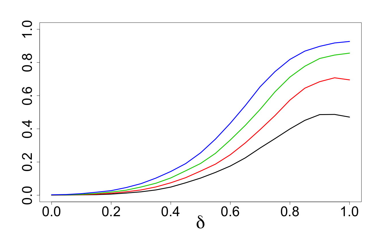
Figure 51: ${C}_{d}(\mathbb{Z}_{n},r)$ for Design S1: $d=5$, $n=128$,
$r$ from $0.11$ to $0.17$ increasing by $0.02$.

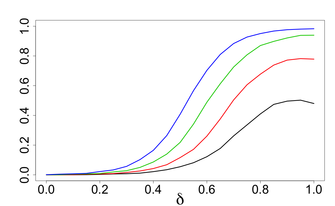
Figure 52: ${C}_{d}(\mathbb{Z}_{n},r)$ for Design S1: $d=10$, $n=512$,
$r$ from $0.13$ to $0.19$ increasing by $0.02$.

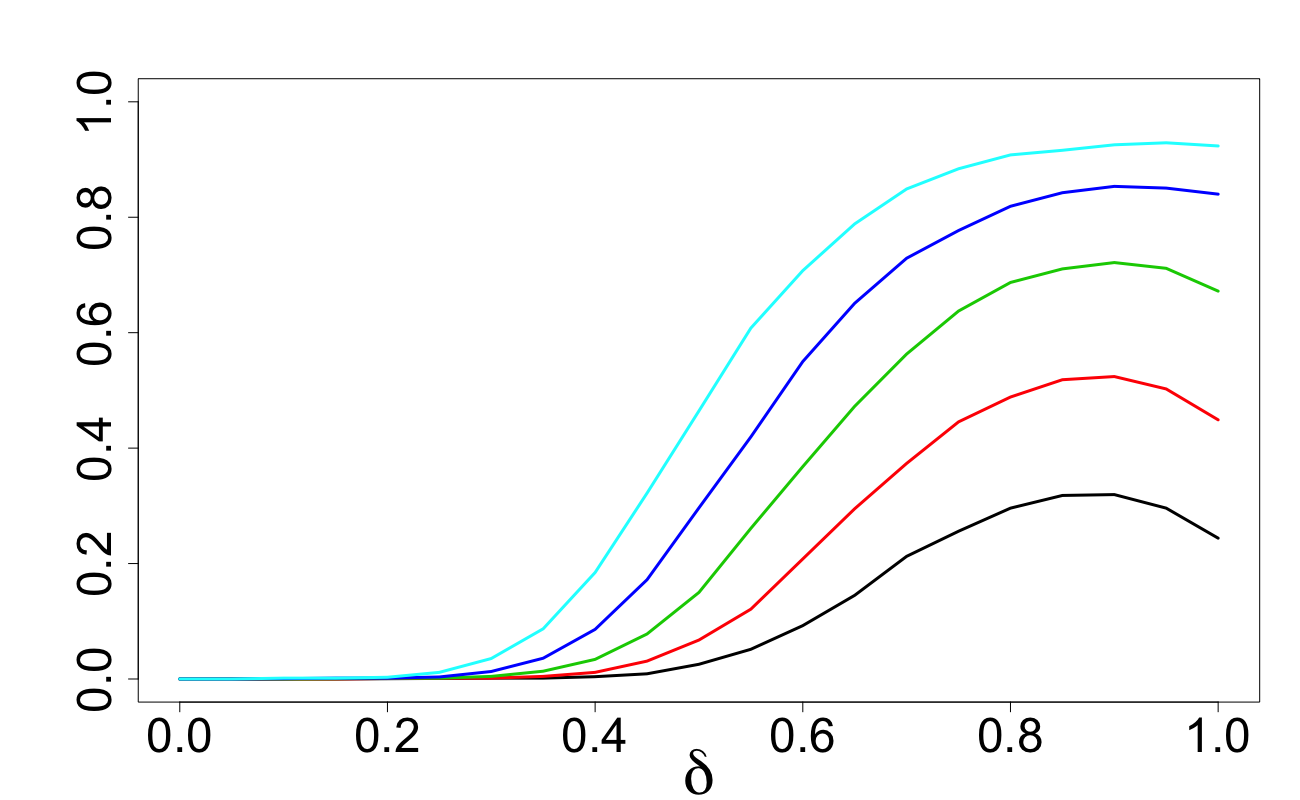
Figure 53: ${C}_{d}(\mathbb{Z}_{n},r)$ for Design S1: $d=20$,
$n=1024$, $r$ from $0.13$ to $0.17$ increasing by $0.01$.

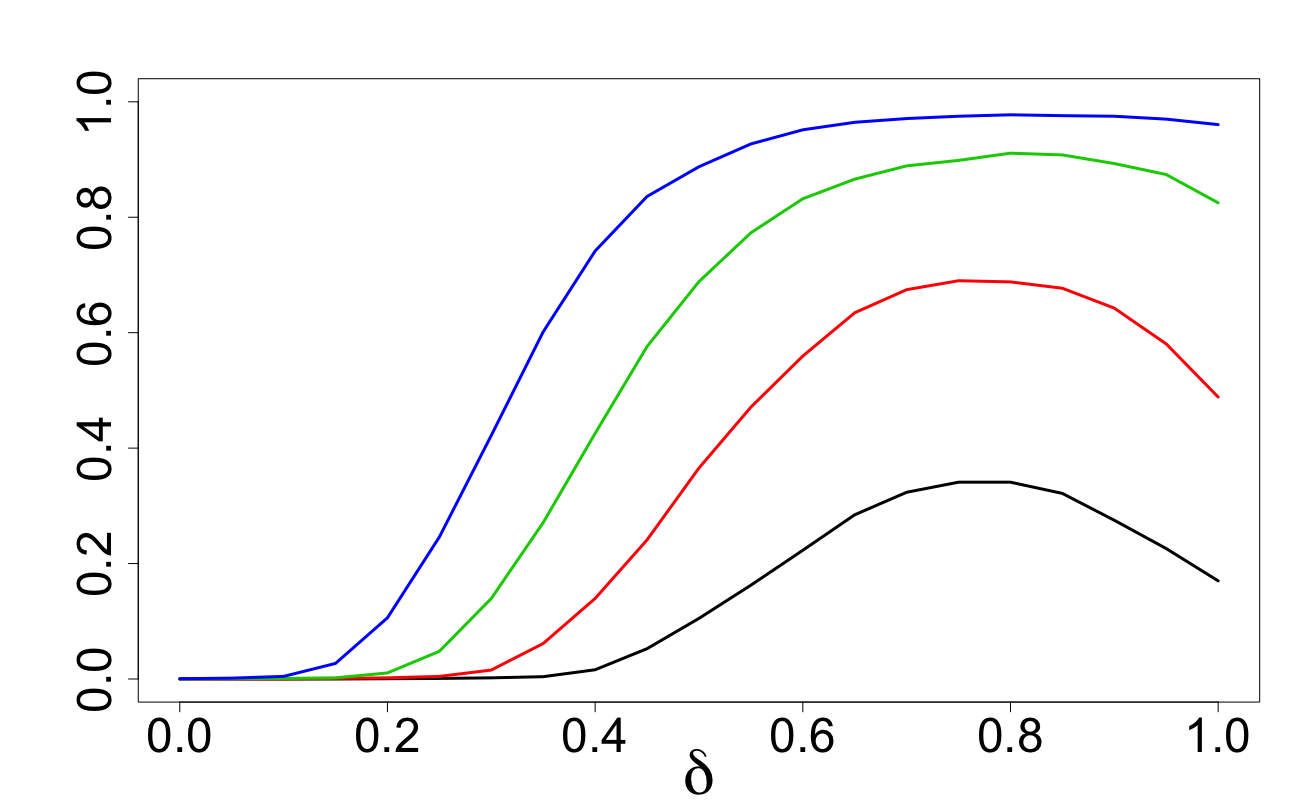
Figure 54: ${C}_{d}(\mathbb{Z}_{n},r)$ for Design S1: $d=50$, $n=1024$,
$r$ from $0.12$ to $0.15$ increasing by $0.01$.

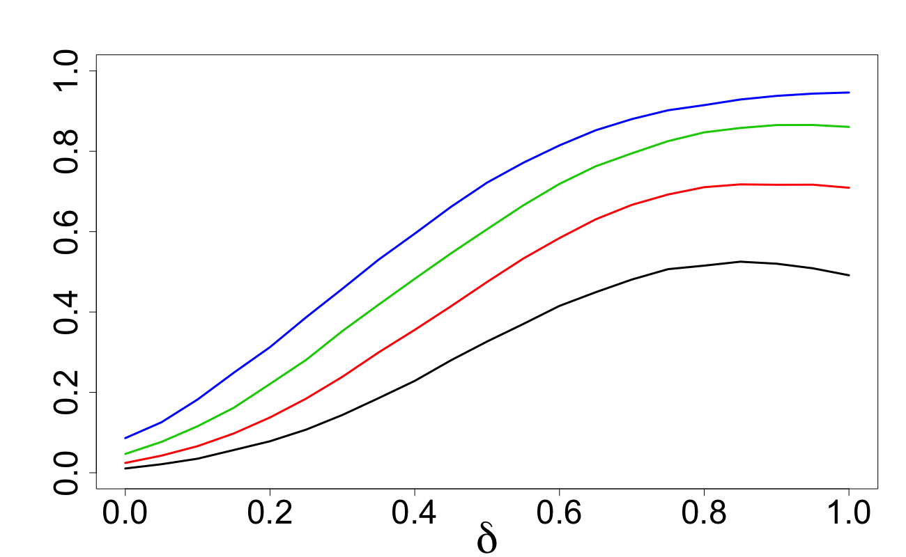
Figure 55: ${C}_{d}(\mathbb{Z}_{n},r)$ for Design S2: $d=5$,
$n=128$, $r$ from $0.11$ to $0.17$ increasing by $0.02$.

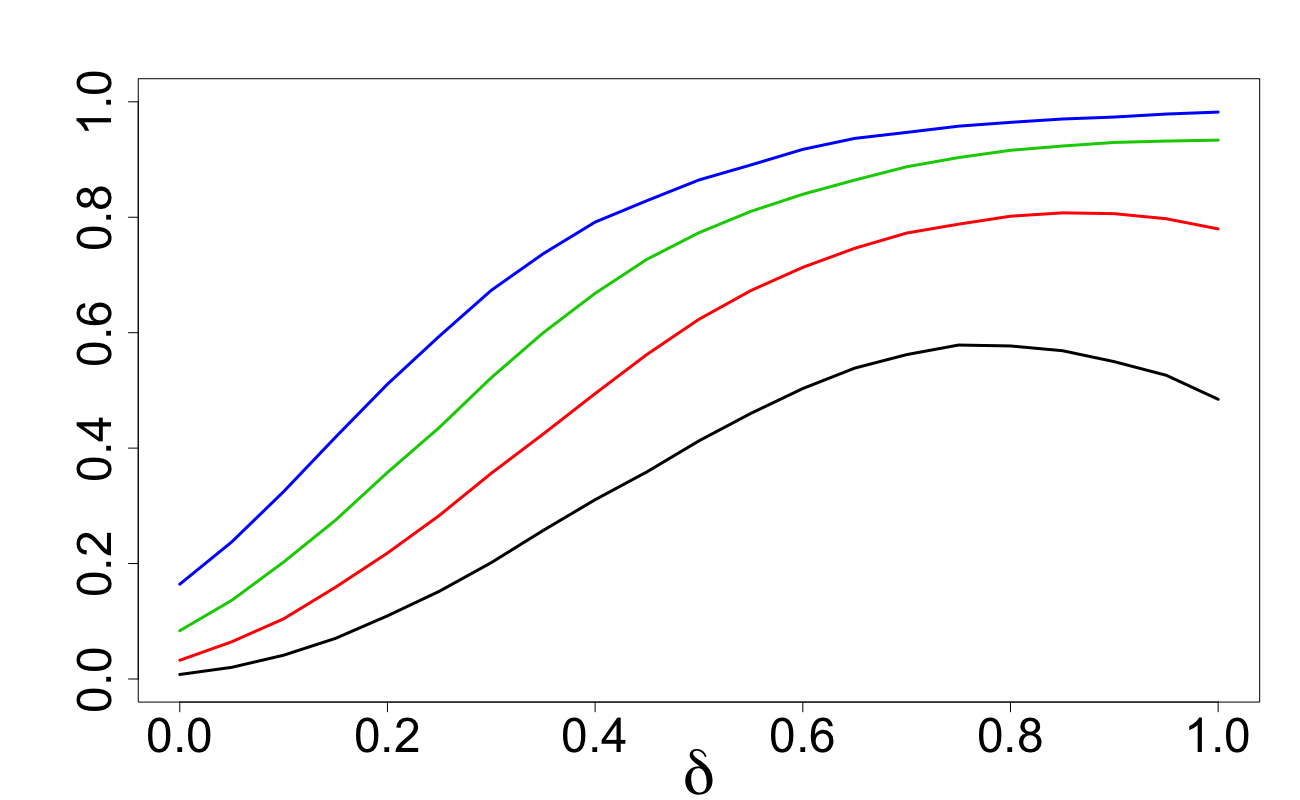
Figure 56: ${C}_{d}(\mathbb{Z}_{n},r)$ for Design S2: $d=10$, $n=512$,
$r$ from $0.13$ to $0.19$ increasing by $0.02$.

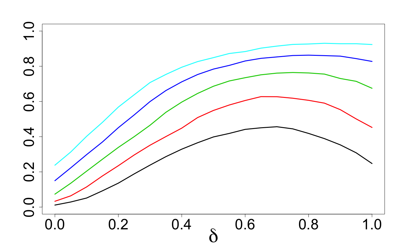
Figure 57: ${C}_{d}(\mathbb{Z}_{n},r)$ for Design S2: $d=20$,
$n=1024$, $r$ from $0.13$ to $0.17$ increasing by $0.01$.

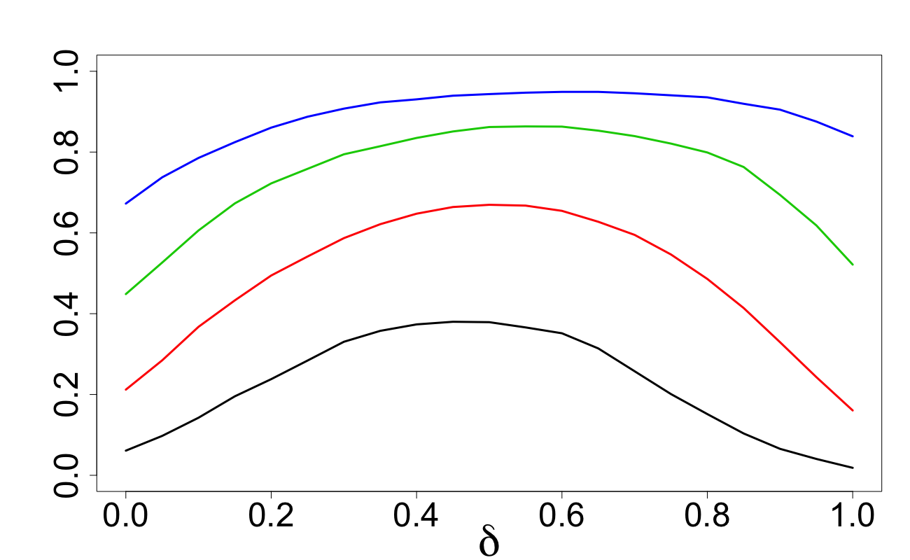
Figure 58: ${C}_{d}(\mathbb{Z}_{n},r)$ for Design S2: $d=50$, $n=1024$,
$r$ from $0.11$ to $0.14$ increasing by $0.01$.

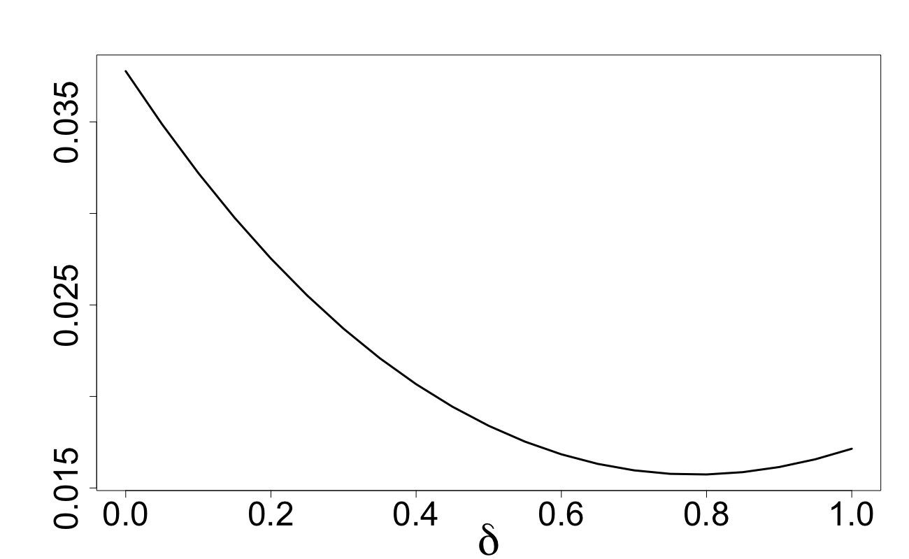
Figure 60: $\mathbb{E}\theta(\mathbb{Z}_{n})$ for Design S1: $d=50$, $n=1024$.

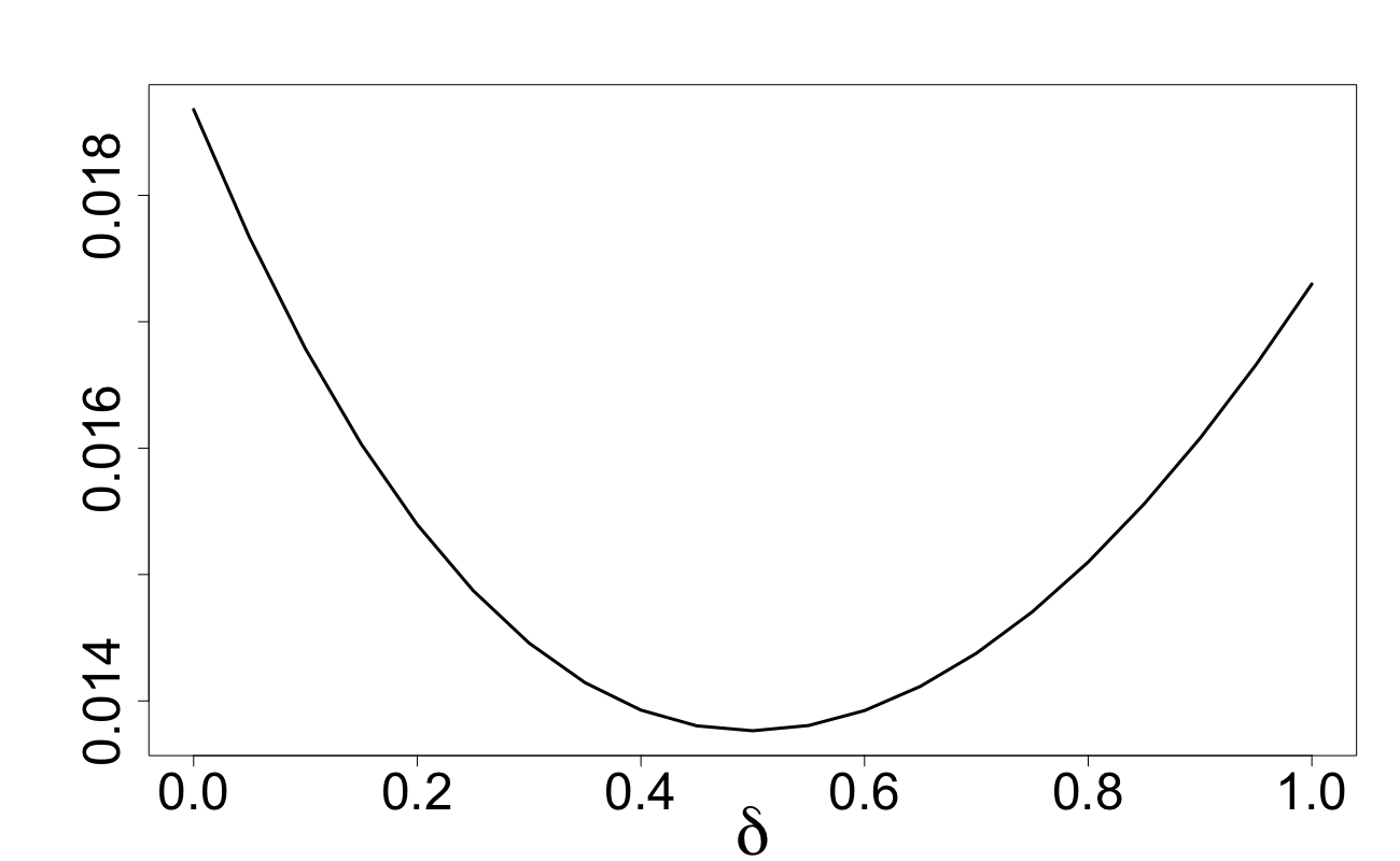
Figure 62: $\mathbb{E}\theta(\mathbb{Z}_{n})$ for Design S2: $d=50$, $n=1024$.

From the above figures, we arrive at the following conclusions:

• The $\delta$-effect for the simplex is much less prominent than for the cube.

• Between Designs S1 and S2, the $\delta$-effect is more apparent for Design S2; for example, compare Figure 60 with Figure 62.

10 Appendix: An auxiliary lemma

Lemma 1. Let $\delta>0$, $u\in\mathbb{R}$ and $\eta_{u,\delta}$ be a r.v. $\eta_{u,\delta}=(\xi-u)^{2}$, where r.v. $\xi\in[-\delta,\delta]$ has Beta${}_{\delta}(\alpha,\alpha)$ distribution with density

$$p_{\alpha,\delta}(t)=\frac{(2\delta)^{1-2\alpha}}{\mbox{Beta$(\alpha,\alpha)$}}[\delta^{2}-t^{2}]^{\alpha-1}\,,\;\;-\delta<t<\delta\,,\alpha>0;$$ (37)

Beta$(\cdot,\cdot)$ is the Beta-function. The r.v. $\eta_{u,\delta}$ is concentrated on the interval $[(\max(0,\delta-|u|))^{2},(\delta+|u|)^{2}]$. Its first three central moments are:

$$\mu_{u,\delta}^{(1)} = E\eta_{u,\delta}=u^{2}+\frac{{{\delta}}^{2}}{2\,{\alpha}+1}\,,$$

$$\mu_{u,\delta}^{(2)} = {\rm var}(\eta_{u,\delta})={\frac{4\delta^{2}}{2\,{\alpha}+1}}\left[u^{2}+{\frac{{{\delta}}^{2}{\alpha}}{\left(2\,{\alpha}+1\right)\left(2\,{\alpha}+3\right)}}\right]\,,$$

$$\mu_{u,\delta}^{(3)} = E\left[\eta_{u,\delta}-E\eta_{u,\delta}\right]^{3}={\frac{48{\alpha}\,{{\delta}}^{4}}{\left(2\,{\alpha}+1\right)^{2}\left(2\,{\alpha}+3\right)}}\left[u^{2}+{\frac{{{\delta}}^{2}\left(2\,{\alpha}-1\right)}{3\left(2\,{\alpha}+5\right)\left(2\,{\alpha}+1\right)}}\right]\,.$$

In the limiting case $\alpha=0$, where the r.v. $\xi$ is concentrated at two points $\pm\delta$ with equal weights, we obtain: $\mu_{u,\delta}^{(1)}=E\eta_{u,\delta}=u^{2}+\delta^{2}\,$ and

$$\mu_{u,\delta}^{(2k)}=\left[2\delta u\right]^{2k},\;\;\;\mu_{u,\delta}^{(2k+1)}=0,\;\;{\rm for}\;\;k=1,2,\ldots$$ (38)

References

- [1] J. Conway and N. Sloane. Sphere packings, lattices and groups. Springer Science & Business Media, 2013.
- [2] M. E. Johnson, L. M. Moore, and D. Ylvisaker. Minimax and maximin distance designs. Journal of statistical planning and inference, 26(2):131–148, 1990.
- [3] H. Niederreiter. Random number generation and quasi-Monte Carlo methods. SIAM, 1992.
- [4] J. Noonan and A. Zhigljavsky. Covering of high-dimensional cubes and quantization. SN Operations Research Forum, to appear, arXiv preprint arXiv:2002.06118, 2020.
- [5] J. Noonan and A. Zhigljavsky. Efficient quantization and weak covering of high dimensional cubes. arXiv preprint arXiv:2005.07938, 2020.
- [6] V. V. Petrov. Sums of independent random variables. Springer-Verlag, 1975.
- [7] V. V. Petrov. Limit theorems of probability theory: sequences of independent random variables. Oxford Science Publications, 1995.
- [8] B.L.S. Prakasa Rao. Asymptotic theory of statistical inference. Wiley, 1987.
- [9] L. Pronzato and W. G. Müller. Design of computer experiments: space filling and beyond. Statistics and Computing, 22(3):681–701, 2012.
- [10] A Sukharev. Minimax models in the theory of numerical methods. Springer Science & Business Media, 1992.
- [11] A. G. Sukharev. Optimal strategies of the search for an extremum. USSR Computational Mathematics and Mathematical Physics, 11(4):119–137, 1971.
- [12] G. F. Tóth. Packing and covering. In Handbook of discrete and computational geometry, pages 27–66. Chapman and Hall/CRC, 2017.
- [13] G. F. Tóth and W. Kuperberg. Packing and covering with convex sets. In Handbook of Convex Geometry, pages 799–860. Elsevier, 1993.
- [14] A. Žilinskas. On the worst-case optimal multi-objective global optimization. Optimization Letters, 7(8):1921–1928, 2013.