Global Optimization of Relay Placement for
Seafloor Optical Wireless Networks

Abstract

Optical wireless communication is a promising technology for underwater broadband access networks, which are particularly important for high-resolution environmental monitoring applications. This paper focuses on a deep-sea monitoring system, where an underwater optical wireless network is deployed on the seafloor. We model such an optical wireless network as a general queueing network and formulate an optimal relay placement problem, whose objective is to maximize the stability region of the whole system, i.e., the supremum of the traffic volume that the network is capable of accommodating. The formulated optimization problem is further shown to be non-convex, so that its global optimization is non-trivial. In this paper, we develop a global optimization method for this problem and we provide an efficient algorithm to compute an optimal solution. Through numerical evaluations, we show that a significant performance gain can be obtained by using the derived optimal solution.

Keywords: Underwater communication, Visible light, Optical network, Queueing network, Global optimization, Reverse convex programming.

1 Introduction

Real-time monitoring of underwater environments, such as ocean trenches and submarine volcanoes, is of great importance for scientific research toward the prevention and mitigation of natural disasters. In such monitoring applications, underwater wireless communication is a key enabling technology for bringing data from seafloor sensors to terrestrial base stations [1]. Traditionally, acoustic signals have been the primary medium for underwater wireless communications due to their ability to propagate over long distances with little energy dissipation. However, the main weakness of the acoustic channel is the quite limited data transmission capacity, which is inherent in the use of kHz-class carrier frequencies. Therefore, acoustic-based underwater communication networks cannot accommodate the large amount of traffic generated by high-specification sensors such as underwater LIDARs and video cameras [2], which will be essential for near-future real-time underwater monitoring systems.

Underwater optical wireless communication (UOWC) is a promising solution to this problem, which can achieve data rates of several hundred Mbps to about ten Gbps, provided that the transmission range is limited to tens to hundreds of meters [3, 4]. Because of this limitation on the propagation distance, it is necessary for the practical use of UOWC to construct a networked optical wireless infrastructure consisting of multiple relay nodes. Such an underwater network is called an underwater optical wireless network (UOWN), and its optimal design has become a major challenge for realizing underwater real-time monitoring applications. Although a wired link (optical fiber) can also be considered as a connection method between relay nodes, this paper focuses on a relay system that is interconnected with wireless optical communication, because the ease of relocation provides operational flexibility desirable for seafloor monitoring systems that are currently under development.

Motivation

Most previous works on UOWNs assume vertical network architectures [4, 5, 6, 7, 8, 9], where data packets generated by seafloor sensors are transferred to a terrestrial base station in multi-hop fashion via vertically deployed optical wireless relay nodes. In such a vertical network architecture, autonomous underwater vehicles (AUVs) hovering in the water are inevitably used as relay nodes in addition to those anchored to the seafloor.

Such architectures with relay AUVs are targeted at relatively shallow marine environments with depths not exceeding 1000 meters, and their use for deep-sea monitoring is impractical due to the following two reasons. Firstly, the monitoring of deep-sea environments with a vertical network requires a very large number of AUV relay nodes to connect seafloor sensors to nodes at the sea surface, resulting in enormous costs. Secondly, the AUV relay nodes must be controlled to keep hovering in the turbulent water, making it difficult to keep all the links stable. To the best of our knowledge, there has not been sufficient attention paid to investigating network architectures that can solve these problems of deep-sea environment monitoring.

Contributions

This paper proposes a seafloor optical wireless network (SOWN), which enables efficient data acquisition from deep-seafloor environments without employing hovering AUV relay nodes. The main components of the proposed SOWN are (i) a terrestrial base station, (ii) a sink node on the seafloor connected to the terrestrial base station with an optical fiber, and (iii) anchored relay nodes horizontally deployed on the seafloor; see Fig. 1 for an illustration. The SOWN serves as an infrastructure to accommodate data traffic originating from a variety of sensors on the seafloor. The sensing data generated by each sensor is first collected at the nearest relay node, then delivered to the sink node by optical wireless multi-hop transmission, and then transferred to the terrestrial base station via the optical fiber. Its main advantage being constructed without hovering AUV nodes, the SOWN is a suitable network architecture for deep-sea monitoring systems in terms of the cost-effectiveness and stability.

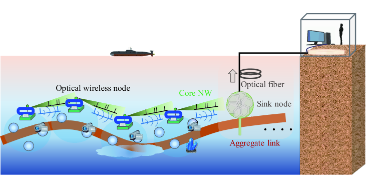
Figure 1: A seafloor optical wireless network.

The main focus of this paper is on the development of an optimal relay placement method, which is the most fundamental challenge toward the optimal design of the SOWN. Underwater relay-node placement problems have traditionally been discussed for acoustic-based networks [10, 11, 12, 13], where it is known to be optimal to use a constant relay spacing [10], provided that the carrier frequency is appropriately selected. The key observation in this paper, however, is that such a constant-spaced relay placement cannot fully extract the transmission capacity of the whole network in the SOWN, but rather a placement with optimally determined non-constant node spacing significantly improves the network performance. Such an improvement basically stems from the fact that the capacity of an underwater optical channel is significantly affected by the node distance, due to the rapid attenuation of the optical signal with propagation distance [14, 15, 16]. In order to efficiently utilize the resources of the whole network, it is then necessary to arrange relay nodes in such a way that the distance between the nodes gradually increases from the sink node to the end (leaf) node, because optical wireless links close to the sink node have to relay a large amount of sensing data transferred from upstream nodes and require a larger channel capacity than those away from the sink node.

In this paper, we make this idea concrete by modeling the relay placement in the SOWN mathematically and performing its detailed analysis. More specifically, we first introduce a queueing-network model whose input process differs depending on the relay-node placement, under a mild assumption that the packet generation follows a general stationary point process. Using this model, we then formulate an optimal relay placement problem that aims to maximize the stability region of the whole system. The stability region is defined as the range of total traffic load that the network can accommodate without exceeding the capacity of any communication links, which is of primary importance in designing communication networks because it determines the fundamental performance limit of the system as well known in the queueing theory.

The main technical challenge we have to address in this relay placement problem is that the formulated optimization problem is inherently non-convex, as will be shown later. Therefore its global optimization is non-trivial, and general-purpose off-the-shelf algorithms can basically yield only local optimal values. In this paper, we perform a detailed theoretical analysis of the optimal relay placement problem and develop a global optimization algorithm that can be executed quite efficiently.

As an initial study of the relay placement problem in the SOWN, this paper mainly focuses on a one-dimensional network, i.e., the case where relay nodes are placed along a straight line. Although this assumption may restrict the direct applicability of the results to be obtained, this simplification allows us to reveal the exact structural properties of the global optimal solution, as will be shown in this paper. Since the one-dimensional network is a fundamental building block of a more general two- or three-dimensional UOWNs, the mathematical analysis developed in this paper also provides theoretical insights into the network design of such general UOWNs; we shall later demonstrate how the mathematical results obtained for the one-dimensional network can be extended to the two-dimensional case. It is also worth noting that the one-dimensional SOWN itself has important practical applications for mitigating natural disasters (particularly earthquakes), such as high-resolution real-time monitoring of ocean trenches.

Organization

The rest of this paper is organized as follows. In Section 2, we provide a brief review of previous studies related to UOWNs and relay placement problems. In Section 3, we introduce a queueing-network model representing the SOWN and formulate an optimal relay placement problem based on it. In Section 4, we develop a global optimization method for the relay placement problem and investigate the mathematical structure of the obtained optimal solution. In Section 5, we first examine the performance of the obtained optimal solution through extensive numerical experiments. In particular, we show that the optimal placement with non-constant spacing significantly improves the system performance compared to the constant spacing case. We then demonstrate an extension of the obtained results to a two-dimensional seafloor network. Finally, this paper is concluded in Section 6.

2 Related works

Gbps-class transmission capacity in UOWC has been achieved by using visible light bands, where the effects of absorption and scattering losses are relatively small. UOWC is still in the early stages of development, and several demonstration experiments have been carried out in recent years [17, 18, 19, 20, 21]. On the other hand, theoretical investigations on UOWC channel characteristics have been carried out from earlier years, and various channel models have been proposed. Giles and Bankman [14] derived a basic signal-to-noise ratio (SNR) formula for UOWC channels, which was further extended to an end-to-end signal strength model by Doniec et al. [15], where its validity was confirmed in a real system. Elamassie et al. [16] have also extended this SNR formula and proposed a correction that takes into account the contribution of the scattered light that partially reaches the detector. For a more detailed characterization of the UOWC channel, Tang et al. [22] have proposed a channel impulse response model with a double gamma function. Jaruwatanadilok [23] has developed a channel model based on radiative transfer theory as well and Zhang et al. [24] have presented a stochastic channel model representing the spatiotemporal probability distribution of propagating photons, taking into account the non-scattering, single-scattering, and multiple-scattering components.

From the perspective of UOWC networking, Akhoundi et al. [25] have introduced an optical code-division multiple access (CDMA) underwater cellular network and evaluated its performance in several water types. Optical CDMA underwater networks have been further studied by Jamali et al. [26], reflecting the turbulent behavior of underwater channels. Jamali et al. [27] have also presented the benefits of serial relayed multi-hop transmission using a bit detection and transfer (BDF) strategy, showing that multi-hop transmission can significantly improve system performance by mitigating adverse effects on all channels. Vavoulas et al. [28] have studied an effective path loss model in UOWC and characterized the connectivity of long-distance underwater communications. Saeed et al. have analyzed network localization performances in terms of the network connectivity in [8] and proposed a localization framework for energy harvesting nodes in [9]. In [29], they have also discussed an optimal placement of seaface anchor nodes in terms of the localization accuracy. To evaluate the performance of a video streaming under the sea, Al-Halafi et al. [30] have modeled UOWC channels with M/G/1 queues, assuming that there are multiple laser diodes in the transmitter and multiple avalanche photodiodes in the receiver. Celik et al. [5] have analyzed the end-to-end bit error rates for the decode and forward (DF) and amplify and forward (AF) relaying in a vertical UOWN. Furthermore, in [6], a sector-based opportunistic routing protocol has been devised where packets are transmitted simultaneously to multiple relay nodes that fall within the range of a directional beam. Xing et al. [31] have investigated problems of minimizing energy consumption and maximizing SNR by performing relay node selection and power allocation simultaneously in the AF scheme.

As mentioned earlier, relay-node placement under water has been studied in the context of acoustic communication systems. Kam et al. [10] considered a problem of optimizing the frequency and node location to minimize the energy consumption. Souza et al. [11] considered the minimization of energy consumption taking into account the optimal number of hops, retransmission, coding rate, and SNR, where the distance between nodes of each hop is assumed to be constant. Liu et al. [12] have developed flow assignment and relay node placement methods in a vertical UOWN to maximize network lifetime, where it is assumed that relay nodes are fixed in horizontal coordinates and can be changed only in vertical coordinates. Prasad et al. [13] have discussed a problem for a two-hop network that minimizes the probability of receiving power falling below an outage-data-rate threshold by properly controlling the locations of relay nodes and the transmission power.

3 Model

Throughout the paper, we follow the convention that for any $k$-dimensional ($k=1,2,\ldots$) vector $\bm{y}\in\mathbb{R}^{k}$, its $i$th element is denoted by $y_{i}$. We further define empty sum terms as zero.

Let $\mathcal{N}=\{1,2,\ldots,N\}$ ($N=1,2,\ldots$) denote the set of relay nodes. Relay nodes are aligned on a subset $\mathcal{L}:=[0,L]$ of the real half-line $\mathbb{R}^{+}$, and the sink node is placed at the origin $x=0$. Let $x_{n}$ ($n=1,2,\ldots,N$) denote the position of the $n$th node. We assume $0\leq x_{n}\leq x_{n+1}$ ($n=1,2,\ldots,N-1$) without loss of generality. We call the sink node ‘the $0$th’ node, so that $x_{0}:=0$ is defined accordingly. We assume that $x_{N}=L$ holds and that the one-dimensional region $\mathcal{L}$ is completely covered by the sink node and $N$ relay nodes as described below.

We assume that generation times of data packets follow a general stationary point process and that the generation points of those packets are uniformly distributed on $\mathcal{L}$. Each packet is first collected by the nearest node from its generation point and then transferred to the sink node with multi-hop transmissions. More formally, we define the coverage area $\mathcal{C}_{n}\subseteq\mathbb{R}^{+}$ ($n=0,1,\ldots,N$) of the $n$th node as its Voronoi cell, which is given by a half-open interval $\mathcal{C}_{n}=[a_{n},b_{n})$ with

$$a_{0}=0,\;\;a_{n}=\frac{x_{n-1}+x_{n}}{2},\;n=1,2,\ldots,N,\quad b_{n}=a_{n+1},\;n=0,1,\ldots,N-1,\;\;b_{N}=x_{N}.$$ (1)

See Fig. 3 for an illustration. Clearly we have $\cup_{n=0}^{N}\mathcal{C}_{n}=[0,x_{N})$ and $\mathcal{C}_{i}\cap\mathcal{C}_{j}=\emptyset$ for $i\neq j$. We further assume that packet transmissions are performed in the store-and-forward manner (DF relaying, in other words). The system is then represented as a network of $N$ G/G/1 queues depicted in Fig. 3, where $\lambda$ denotes the mean number of generated packets per unit time (within the whole covered area $\mathcal{L}$) and $B$ denotes the mean data size.

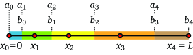
Figure 2: An illustration of the system model ($N=4$).

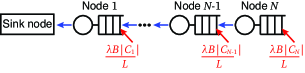
Figure 3: The SOWN modeled as a network of G/G/1 queues.

We define $\rho_{n}$ ($n=1,2,\ldots,N$) as the traffic intensity of external arrivals to the $n$th node, i.e.,

$$\rho_{n}=\frac{\lambda|\mathcal{C}_{n}|}{L}\cdot B=q|\mathcal{C}_{n}|,\qquad q:=\frac{\lambda B}{L}.$$ (2)

Observe that $q$ represents the amount of data brought into the system per unit time, normalized by the area length. Owing to [32, Page 142], the stability condition of this system is given by that for each node $i$, the total traffic intensity of relayed packets does not exceed the link capacity:

$$\sum_{n=i}^{N}\rho_{n}<R(d_{i}),\;\;i\in\mathcal{N},$$ (3)

where $d_{n}:=x_{n}-x_{n-1}$ ($n=1,2,\ldots$) denotes the distance between the ($n-1$)st and $n$th nodes, and $R(d)$ ($d\geq 0$) denotes the effective transmission rate between two nodes with distance $d$, which is formulated as follows.

Let $\mathrm{SNR}(d)$ ($d\geq 0$) denote the electrical SNR at distance $d$. A widely used model [14, 15, 16, 31, 33] for representing the SNR of a UOWC channel is that the $\mathrm{SNR}(d)$ takes a form proportional to $d^{-\alpha}e^{-Kd}$ for some coefficients $\alpha>0$ and $K>0$. In this expression, $d^{-\alpha}$ represents the signal attenuation due to the geometric spreading of the light beam and $\alpha=2$ is usually used to represent the spherical spreading. On the other hand, $e^{-Kd}$ represents the contribution of absorption and scattering losses, and $K$ is given by the sum of the absorption and scattering coefficients, which vary depending on the type of water and the light wavelength. Readers are referred to [3, 7, 15, 34] for more detailed explanations on such a theoretical characterization and its validation in a real system.

In this paper, to avoid the singularity of $d^{-\alpha}$ at the origin, we consider the following bounded expression for $\mathrm{SNR}(d)$, with a small $\epsilon>0$:

$$\mathrm{SNR}(d)=Ae^{-Kd}(\epsilon+d)^{-\alpha},$$ (4)

where $A$ denotes a constant that depends on physical parameters (an example will be given later in Section 5). It should be noted here that $\epsilon$ does not have a specific physical meaning: it is a parameter intended to correct the singular behavior that $d^{-\alpha}$ diverges near the origin, and the value of $\epsilon$ has little effect on $\mathrm{SNR}(d)$ unless $d$ is very small (such a correction term is often used in the radio communication literature [35]). Owing to the Shannon-Hartley theorem, with $W$ denoting the bandwidth, the effective transmission rate $R(d)$ ($d\geq 0$) is then expressed as

$$R(d)=W\log(1+\mathrm{SNR}(d)).$$ (5)

In order not to restrict the applicability of our theoretical results, however, we do not assume any specific expression for the function $R(d)$ in performing mathematical analysis below. Instead, we make only the following assumption on $R(d)$, which is clearly satisfied by (4) and (5):

Assumption 1.

The effective transmission rate $R:[0,\infty)\rightarrow[0,\infty)$ is a strictly decreasing, continuously differentiable convex function of the node distance, and $\lim_{d\to\infty}R(d)=0$.

Remark 2.

Another example of an expression for $R(d)$ (other than the Shannon capacity (5)) is given as follows. Suppose that sensing information is coded and modulated with (i) the modulation level $M$ [bits/symbol] and (ii) a forward-error-correction (FEC) code with code rate $\eta$ ($0<\eta<1$). Also suppose that the FEC code enables the receiver to decode the signal with a negligible error-rate, provided that the SNR does not exceed a threshold $\zeta$. This is an abstraction of UOWC channels implemented with standard modulation techniques, such as the on-off keying (OOK) and the quadrature amplitude modulation (QAM) [36].

In this setting, it is reasonable that the transmitter uses the maximum symbol rate (which equals the bandwidth $W$) such that the constraint $\mathrm{SNR}(d)\leq\zeta$ for error-free transmission is satisfied. Assuming that the noise spectral density is constant (i.e., white noise) over the operating frequency range, the expression (4) is rewritten as $\mathrm{SNR}(d)=A^{\prime}e^{-Kd}(\epsilon+d)^{-\alpha}W^{-1},$ where $A^{\prime}$ does not depend on the symbol rate $W$. $\mathrm{SNR}(d)$ then decreases with $W$, so that the maximum symbol rate is achieved if (and only if) $\mathrm{SNR}(d)=\zeta$, i.e., $W=A^{\prime}e^{-Kd}(\epsilon+d)^{-\alpha}\zeta^{-1}.$ As the effective transmission rate equals $\eta\cdot M\cdot W$, we then conclude $R(d)=\eta MA^{\prime}e^{-Kd}(\epsilon+d)^{-\alpha}\zeta^{-1},$ which clearly satisfies Assumption 1.

Remark 3.

A refinement of the SNR equation correcting the exponential term as $e^{-Kd^{\beta}}$ ($\beta\in(0,1]$) is proposed in [16]; the discussion above is still valid under such an extension.

We see from (2) and (3) that the stability region of the system varies depending on the node placement $\bm{x}:=(x_{1},x_{2},\ldots,x_{N})^{\top}$. Let $\rho_{n}(q,\bm{x})$ ($n=1,2,\ldots,N$) denote the traffic intensity $\rho_{n}$ of external arrivals to the $n$th node, represented as a function of the normalized traffic intensity $q$ and the placement of relay nodes $\bm{x}$ (cf. (2)). The size of the stability region is characterized by the normalized throughput limit $q_{\sup}(\bm{x})$, which is defined as the least upper bound of the normalized throughput $q$ for which the system is stable:

$$q_{\sup}(\bm{x}) =\sup\biggl{\{}q\in\mathbb{R}^{+}\ \biggl{|}\ \sum_{n=i}^{N}\rho_{n}(q,\bm{x})<R(x_{i}-x_{i-1}),\,i\in\mathcal{N}\biggr{\}}$$

$$=\max\biggl{\{}q\in\mathbb{R}^{+}\ \biggl{|}\ \sum_{n=i}^{N}\rho_{n}(q,\bm{x})\leq R(x_{i}-x_{i-1}),\,i\in\mathcal{N}\biggr{\}}.$$ (6)

The size of the stability region (i.e., the value of the normalized throughput limit $q_{\sup}(\bm{x})$) is the most fundamental performance metric in designing the communication network. In this paper, we thus employ $q_{\sup}(\bm{x})$ as the objective function of our optimal placement problem. Specifically, we develop a solution method to the following optimization problem:

$$\underset{\bm{x}\in\mathbb{R}^{N}}{\mathrm{maximize}}\;\;q_{\sup}(\bm{x})\quad\mathrm{s.t.}\;\;x_{N}=L,\;\;x_{i+1}\geq x_{i}\geq 0,\;\;i\in\{1,2,\ldots,N-1\},$$

which is rewritten as (cf. (6))

$$\underset{q\in\mathbb{R},\,\bm{x}\in\mathbb{R}^{N}}{\mathrm{maximize}}\;\;q\quad\mathrm{s.t.}\;\; \sum_{n=i}^{N}\rho_{n}(q,\bm{x})\leq R(x_{i}-x_{i-1}),\;\;i\in\{1,2,\ldots,N\},$$

$$x_{N}=L,\;\;x_{i+1}\geq x_{i},\;\;i\in\{1,2,\ldots,N-1\},$$

$$q\geq 0,\;\;x_{i}\geq 0,\;\;i\in\{1,2,\ldots,N\}.$$ (U₀)

Note that an optimal solution of (U₀) provides not only an optimal placement $\bm{x}^{*}$ of relay nodes but also the achievable maximum value of the normalized throughput limit $q_{\sup}^{*}:=q_{\sup}(\bm{x}^{*})$.

4 Global optimization method

In this section, we develop a global optimization method for (U₀). We start with rewriting (U₀) into a more comprehensive form. We have from (1) and (2),

$$\rho_{n}(q,\bm{x})=\frac{q(x_{n+1}-x_{n-1})}{2},\;\;n=1,2,\ldots,N-1,\quad\rho_{N}(q,\bm{x})=\frac{q(x_{N}-x_{N-1})}{2},$$ (7)

so that we can rewrite (U₀) in terms of the distance $d_{n}=x_{n}-x_{n-1}$ ($n=1,2,\ldots,N$) of nodes:

$$\underset{q\in\mathbb{R},\,\bm{d}\in\mathbb{R}^{N}}{\mathrm{maximize}}\;\;q\quad\mathrm{s.t.}\;\; R(d_{i})-\frac{qd_{i}}{2}-\sum_{n=i+1}^{N}qd_{n}\geq 0,\;\;i\in\{1,2,\ldots,N\},$$

$$q\geq 0,\;\;\sum_{i=1}^{N}d_{i}=L,\;\;d_{i}\geq 0,\;\;i\in\{1,2,\ldots,N\}.$$ (U)

It is readily verified that (U) does not have a convex feasible region: for fixed $q\geq 0$, each inequality constraint takes the form that a convex function is not less than $0$ (cf. Assumption 1), so that its feasible region is the complement of a convex set. Such constraints are known as reverse-convex constraints, and a class of optimization problems with this type of constraints is called the reverse-convex programming (RCP) [37]. In general, an optimization problem

$$\underset{\bm{y}\in\mathbb{R}^{K}}{\mathrm{maximize}}\;u(\bm{y})\quad\mathrm{s.t.}\;f_{i}(\bm{y})\geq 0,\;\;i=1,2,\ldots,M,$$ (R)

with $K$ variables and $M$ constraints ($M\geq K$) is called RCP if $u$ and $f_{i}$ ($i=1,2,\ldots,M$) are quasi-convex. Note here that any equality constraints of the form $\sum_{k=1}^{K}w_{k}y_{k}=c$ ($c\in\mathbb{R}$, $w_{k}\in\mathbb{R}$) can be translated into the double number of linear (thus reverse-convex) inequality constraints $\sum_{k=1}^{K}w_{k}y_{k}\leq c$ and $\sum_{k=1}^{K}w_{k}y_{k}\geq c$. Due to the non-convexity of its feasible region, global optimization for RCP is not an easy task in general, and various algorithms to find a globally optimal solution have been developed in the literature (see e.g., [37, 38, 39, 40] and references therein). Here we introduce a known theoretical property of RCP, which will be used in our analysis. Let $\mathcal{A}:=\{\bm{y};\,f_{i}(\bm{y})\geq 0\,(i=1,2,\ldots,M)\}$ denote the feasible region of (R) and let $\mathcal{I}(\bm{y}):=\{i\in\{1,2,\ldots,M\};\,f_{i}(\bm{y})=0\}$ ($\bm{y}\in\mathcal{A}$).

Definition 4 (​​[37, Def. 1]).

$\bar{\bm{y}}\in\mathcal{A}$ is called a basic solution of (R) if the matrix with row vectors $\{\nabla f_{i}(\bar{\bm{y}});\,i\in\mathcal{I}(\bar{\bm{y}})\}$ has rank $K$.

Lemma 5 (​​[37, Th. 9]).

If $u$ and $f_{i}$ ($i=1,2,\ldots,M$) are quasi-convex, (R) has an optimal solution which is also basic.

Remark 6.

A basic solution must satisfy at least $K$ constraints with equality. Lemma 5 thus implies that there exists an optimal solution that satisfies at least $K$ constraints with equality.

In what follows, we develop a global optimization method (U) utilizing its special structure. To that end, we first introduce the following subproblem for each $q>0$:

$$\underset{\bm{d}\in\mathbb{R}^{N}}{\mathrm{maximize}}\;\;\sum_{n=1}^{N}d_{n}\quad\mathrm{s.t.}\;\; R(d_{i})-\frac{qd_{i}}{2}-\sum_{n=i+1}^{N}qd_{n}\geq 0,\;\;i\in\{1,2,\ldots,N\},$$

$$d_{i}\geq 0,\;\;i\in\{1,2,\ldots,N\}.$$ (S_q)

The main difference between (U) and (S_q) is that $q$ is not variable but fixed in (S_q). Also, the coverage $\sum_{i=1}^{N}d_{i}$ of relay nodes is to be maximized in (S_q), while it is fixed to be $L$ in (U).

It is readily verified that the subproblem (S_q) still belongs to RCP. Owing to its special structure, however, a globally optimal solution of (S_q) is explicitly obtained. For a fixed $q>0$, we define a function $g_{q}:[0,\infty)\to(-\infty,R(0)/q]$ as

$$g_{q}(x)=\frac{R(x)}{q}-\frac{x}{2},\quad x\geq 0.$$ (8)

From Assumption 1, $g_{q}$ is a strictly decreasing continuous function, so that it has a unique inverse function $g_{q}^{-1}:(-\infty,R(0)/q]\to[0,\infty)$. The following results show that an optimal solution of (S_q) is explicitly constructed in terms of $g_{q}$ and $g_{q}^{-1}$:

Theorem 7.

• If $g_{q}^{-1}(0)\geq g_{q}(0)$, then the following $\bm{d}^{*}$ is an optimal solution of (S_q):

  $$\bm{d}^{*}=(0,0,\ldots,0,g_{q}^{-1}(0))^{\top}\in\mathbb{R}^{k}.$$ (9)

• If $g_{q}^{-1}(0)<g_{q}(0)$, a backward recursion

  $$d_{N}^{*}=g_{q}^{-1}(0),\quad d_{i}^{*}=g_{q}^{-1}\left(\sum_{n=i+1}^{N}d_{n}^{*}\right),\;\;i=1,2,\ldots,N-1$$ (10)

  well-defines $d_{1}^{*},d_{2}^{*},\ldots,d_{N}^{*}$ such that

  $$0<d_{i}^{*}<d_{i+1}^{*},\quad i=1,2,\ldots,N-1,$$ (11)

  and the following $\bm{d}^{*}$ is an optimal solution of (S_q):

  $$\bm{d}^{*}=(d_{1}^{*},d_{2}^{*},\ldots,d_{N}^{*})^{\top}\in\mathbb{R}^{N}.$$ (12)

Remark 8.

The proof of Theorem 7 is somewhat complicated because a careful treatment is necessary to differentiate between the two cases (i) and (ii). Basically, our proof is based on the fact mentioned in Remark 6 that there exists an optimal solution satisfying at least $N$ constraints with equality. Recall that (S_q) has $2N$ constraints: $N$ out of these are of the form $g_{q}(d_{i})\geq\sum_{n=i+1}^{N}d_{n}$ and the others are of the form $d_{i}\geq 0$. The solution (12) satisfies the former with equality for $i=1,2,\ldots,N$ and it has all non-zero elements. On the other hand, the solution (9) has only one non-zero element, and it satisfies $g_{q}(d_{i})>\sum_{n=i+1}^{N}d_{n}$ for $i=2,3,\ldots,N$.

We provide the proof of Theorem 7 in Appendix A.

The optimal solution given in Theorem 7 takes a different form depending on whether or not $g_{q}^{-1}(0)\geq g_{q}(0)$ holds. While it is easy to check if this inequality holds for given $q$, we also have a simple criterion shown in the following lemma, which is useful in the theoretical analysis below:

Lemma 9.

Let $q_{0}$ denote the unique solution of

$$R\left(\frac{R(0)}{q}\right)-\frac{R(0)}{2}=0,\quad q>0.$$ (13)

We then have

$$g_{q}^{-1}(0)\geq g_{q}(0),\;\;\forall q\geq q_{0},\qquad g_{q}^{-1}(0)<g_{q}(0),\;\;\forall q<q_{0}.$$ (14)

Proof.

Because $g_{q}(x)$ is strictly decreasing with respect to $x$,

$$g_{q}^{-1}(0)\geq g_{q}(0)\ \Leftrightarrow\ g_{q}(g_{q}(0))\leq 0\ \Leftrightarrow\ R\left(\frac{R(0)}{q}\right)-\frac{R(0)}{2}\leq 0,$$ (15)

where we used (8) and $q>0$ in the last equality. From Assumption 1, $R(R(0)/q)-R(0)/2$ is continuous and strictly increasing in $q$ and

$$\lim_{q\to 0+}\left[R\left(\frac{R(0)}{q}\right)-\frac{R(0)}{2}\right]=-\frac{R(0)}{2}<0,\quad\lim_{q\to\infty}\left[R\left(\frac{R(0)}{q}\right)-\frac{R(0)}{2}\right]=\frac{R(0)}{2}>0,$$ (16)

so that (13) has the unique solution. Lemma 9 now follows immediately from (15). ∎

We then relate the subproblem (S_q) with the original problem (U). For $q>0$, let $\bm{d}_{q}^{*}:=(d_{q,1}^{*},d_{q,2}^{*},\ldots,d_{q,N}^{*})^{\top}$ denote the optimal solution of (S_q) given in Theorem 7, and let $x_{q,N}^{*}:=\sum_{i=1}^{N}d_{q,i}^{*}$ denote the corresponding optimal value. The following theorem shows that we can obtain a globally optimal solution of (U) by iteratively solving (S_q):

Theorem 10.

• The optimal value $x_{q,N}^{*}$ of (S_q) is a continuous, strictly decreasing function of $q$ with $\lim_{q\to 0+}x_{q,N}^{*}=\infty$ and $\lim_{q\to\infty}x_{q,N}^{*}=0$.

• The optimal value $q_{\sup}^{*}$ of (U) is characterized as follows:

  $$x_{q,N}^{*}>L\ \Leftrightarrow\ q<q_{\sup}^{*},\quad\;x_{q,N}^{*}<L\ \Leftrightarrow\ q>q_{\sup}^{*},\quad\;x_{q,N}^{*}=L\ \Leftrightarrow\ q=q_{\sup}^{*}.$$ (17)

  Furthermore, $(q_{\sup}^{*},\bm{d}_{q_{\sup}^{*}}^{*})$ is an optimal solution of (U).

The proof of Theorem 10 is provided in Appendix B.

An important consequence of Theorem 10 is that a globally optimal solution of (U) is obtained by iteratively solving the subproblem (S_q) with Theorem 7. Theorem 10 (b) indicates that we can judge if a given value of $q>0$ is smaller, equal to, or greater than the optimal value $q_{\sup}^{*}$ of the original problem (U), by comparing the optimal value $x_{q,N}^{*}$ of the subproblem (S_q) with the area length $L$. It also indicates that an optimal placement $\bm{d}^{*}$ for (U) is equal to that for the subproblem (S_q) with $q=q_{\sup}^{*}$, which is explicitly calculated from Theorem 7 once $q_{\sup}^{*}$ is obtained. Theorem 10 (a) ensures (i) the existence of $q$ such that $x_{q,N}^{*}=L$ (equivalently $q=q_{\sup}^{*}$), and (ii) the monotonicity of $x_{q,N}^{*}$ with respect to $q$. Therefore, a standard bisection method enables us to numerically find the value of $q_{\sup}^{*}$, so that we can effectively compute the optimal placement $\bm{d}^{*}$ for the original problem (U); Algorithm 1 summarizes such a procedure.

Algorithm 1 A global optimization algorithm for (U), in which the optimal solution $\bm{d}_{q}^{*}$ and the optimal value $x_{q,N}^{*}$ of (S_q) is computed with Theorem 7.

1:Number of nodes $N$, area length $L$, transmission rate function $R(d)$ ($d\geq 0$), and output precision $\epsilon$.

2:An optimal solution $(q_{\sup}^{*},\bm{d}^{*})$ of (U).

3:Find $q_{\mathrm{low}}$ and $q_{\mathrm{up}}$ satisfying $0<q_{\mathrm{low}}<q_{\mathrm{up}}$, $x_{q_{\mathrm{low}},N}^{*}\geq L$, and $x_{q_{\mathrm{up}},N}^{*}<L$.

4:while $q_{\mathrm{up}}-q_{\mathrm{low}}\geq\epsilon$ do

5:    $q\leftarrow(q_{\mathrm{low}}+q_{\mathrm{up}})/2$.

6:    if $x_{q,N}^{*}\geq L$ then $q_{\mathrm{low}}\leftarrow q$   else $q_{\mathrm{up}}\leftarrow q$.

7:$q_{\sup}^{*}\leftarrow(q_{\mathrm{low}}+q_{\mathrm{up}})/2$ and $\bm{d}^{*}\leftarrow\bm{d}_{q_{\sup}}^{*}$.

Before closing this section, we conduct further investigations on mathematical structures of the obtained optimal solution. Let $q_{\sup}^{*}(L,N)$ ($L>0$, $N=1,2,\ldots$) denote the optimal value $q_{\sup}^{*}$ of the normalized throughput limit, represented as a function of the area length $L$ and the number of relay nodes $N$ for a fixed transmission rate function $R$.

Lemma 11.

For a fixed $N$ ($N=1,2,\ldots$), $q_{\sup}^{*}(L,N)$ is a strictly decreasing function of $L$.

Proof.

Lemma 11 immediately follows from Theorem 10 (a) and (b): $q_{\sup}^{*}(N,L)$ for fixed $N$ is determined by the unique solution of $x_{q,N}^{*}=L,\,q>0$, which is strictly decreasing with $L$. ∎

Theorem 12.

Let $L_{0}:=g_{q_{0}}^{-1}(0)$, where $q_{0}$ is defined in Lemma 9. For any $N=1,2,\ldots$, we have

$$g_{q_{\sup}^{*}(L,N)}^{-1}(0)\geq g_{q_{\sup}^{*}(L,N)}(0),\;\;\forall L\leq L_{0},\quad g_{q_{\sup}^{*}(L,N)}^{-1}(0)<g_{q_{\sup}^{*}(L,N)}(0),\;\;\forall L>L_{0},$$ (18)

i.e., if $L\leq L_{0}$, an optimal node placement for (U) is given by the form (9), and otherwise it is given by the form (12), regardless of the number of nodes $N$.

Proof.

We readily obtain Theorem 12 from Theorem 7 (i), Lemma 9, Theorem 10, and Lemma 11, noting that $q_{\sup}^{*}(L,N)=q_{0}\;\Leftrightarrow\;L=x_{q_{0},N}^{*}=g_{q_{0}}^{-1}(0)$. ∎

Theorem 12 shows that if the area length $L$ is smaller than or equal to $L_{0}$, the normalized throughput limit $q_{\sup}^{*}(L,N)$ is not affected by the number of nodes $N$, i.e., no performance gain can be obtained by increasing the number of relay nodes in that case. On the other hand, if $L\geq L_{0}$, we can verify from Theorem 10 (a) and Theorem 7 (ii) that $q_{\sup}^{*}(L,N)$ strictly increases with the number of nodes $N$.

Finally, we provide a further characterization of the sequence $d_{1}^{*},d_{2}^{*},\ldots,d_{N}^{*}$ defined by (10), restricting our attention to the case $g_{q}^{-1}(0)>g_{q}(0)$ (i.e., $L>L_{0}$ in view of Theorem 12). As shown in Theorem 7, it is optimal to place relay nodes with ascending node intervals in this case. In other words, if one determines node intervals in the reversed order (i.e., the interval between $N$th and $(N-1)$st nodes is determined first), the sequence of optimal node intervals $d_{N}^{*},d_{N-1}^{*},\ldots,d_{1}^{*}$ is decreasing. The following theorem shows that in the optimal placement, the decrease in node intervals is at least exponentially fast:

Theorem 13.

Let $\gamma$ denote a real number given by

$$\gamma=1+(g_{q}^{-1})^{\prime}(g(0))=1+\frac{1}{g_{q}^{\prime}(0)},$$ (19)

where $f^{\prime}$ denotes the derivative of function $f$. If $g_{q}^{-1}(0)>g_{q}(0)$, then $0<\gamma<1$ and

• if $(g_{q}^{-1})^{\prime}(0)>-1$, we have $d_{i}^{*}\leq\gamma^{N-i}d_{N}^{*}$ ($i=1,2,\ldots,N-1$), and

• if $(g^{-1})^{\prime}(0)\leq-1$, we have $d_{i}^{*}\leq\gamma^{N-i-1}d_{N-1}^{*},$ ($i=1,2,\ldots,N-2$).

The proof of Theorem 13 is provided in Appendix C.

5 Performance Evaluation and Extension

In this section, we evaluate the performance of the obtained optimal solution. We first present extensive numerical experiments to illustrate the effectiveness of the optimal solution, focusing on the one-dimensional SOWN discussed so far. We then provide an example of an optimal relay placement problem for a two-dimensional SOWN, which demonstrates how our result can be extended to a more general situation.

Throughout this section, we employ $R(d)$ given in (5) and the following SNR equation [14]:

$$\mathrm{SNR}(d)=\frac{P_{\mathrm{t}}D^{2}\cos{\varphi}}{4(\tan^{2}\theta)P_{\mathrm{n}}}\cdot\frac{e^{-Kr}}{(\epsilon+r)^{2}},$$ (20)

where $P_{\mathrm{t}}$ denotes the transmitter power, $P_{\mathrm{n}}$ denotes the noise power, $D$ denotes the receiver aperture diameter, $\varphi$ denotes the angle between the optical axis of the receiver and the line-of-sight between the transmitter and the receiver, $\theta$ denotes the half-angle transmitter beamwidth, $K$ denotes the beam attenuation coefficient, and $\epsilon$ denotes the constant introduced in (4). For the noise power $P_{\mathrm{n}}$, we employ a constant value representing thermal noise, assuming that the contribution of shot noise to $P_{\mathrm{n}}$ is negligible due to the small power of received optical signals.

Unless otherwise mentioned, we use parameter values summarized in Table 1 as the default values. We consider three different values for the beam attenuation coefficient $K$, reflecting its dependence on the light wavelength [41] (we restrict our attention to the case of pure water, based on empirical evidence [42] in the deep sea). We also set the area length $L=500$ [m] unless otherwise mentioned.

Table 1: Default parameter values in numerical experiments.

Symbol	Unit	Value
$P_{\mathrm{t}}$	Watt	$0.5$
$P_{\mathrm{n}}$	Watt	$2\times 10^{-6}$
$D$	Meter	$0.2$
$\varphi$	Degree	$10$
$\theta$	Degree	$10$
$W$	Hz	$5\times 10^{8}$
$K$	1/Meter	Red light (650 [nm]):                              $3\times 10^{-1}$
		Green light (550 [nm]):                              $7\times 10^{-2}$
		Blue light (450 [nm]):                              $2\times 10^{-2}$
$\epsilon$	Meter	1

5.1 Performance Evaluation of one-dimensional SOWCs

We start with providing an example of the optimal, non-constant node intervals we have obtained. Fig. 4 illustrates the optimal node placement for the case of green light and Fig. 6 shows the corresponding sequence of optimal node intervals $(d_{i}^{*})_{i=1,2,\ldots,N}$ (i.e., Fig. 6 plots the spacings of the placement in Fig. 4). We observe that the optimal node interval $d_{i}^{*}$ is increasing with $i$ and that there is a large difference between the values of $d_{1}^{*}$ and $d_{N}^{*}$. Fig. 6 shows the maximum normalized throughput limit $q_{\sup}^{*}$ (achieved by the optimal relay placement) as a function of the number $N$ of relay nodes for the three wavelengths. We observe that adding a few relay nodes to the network drastically expands the stability region of the system. Fig. 12 shows the maximum normalized throughput limit $q_{\sup}^{*}$ as a function of the area length $L$ for the blue light. For large values of $L$, we observe that $q_{\sup}^{*}$ exponentially decreases as $L$ increases. Furthermore, for relatively small values of $L$, only little difference can be seen between the values of $q_{\sup}^{*}$ for the number of nodes $N=5$, $N=10$, and $N=20$, and they coincide each other for quite small $L$, i.e., no performance gain can be obtained by using additional relay nodes (cf. Theorem 12).

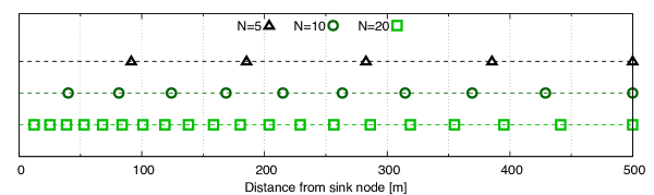
Figure 4: An illustration of the optimal placement of relay nodes for the green light, where each symbol represents a relay node.

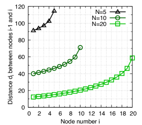
Figure 5: Optimal distances $\{d_{i}\}_{i=1,2,\ldots,N}$ between relay nodes for the green light.

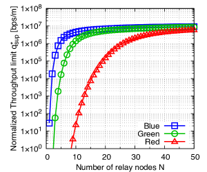
Figure 6: Impact of the number of relay nodes $N$ on the normalized throughput limit $q_{\sup}^{*}$.

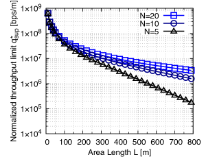
Figure 7: The normalized throughput limit $q_{\sup}^{*}$ as a function of coverage length $L$.

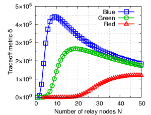
Figure 8: The tradeoff metric $\delta$ as a function of the number $N$ of relay nodes.

Figure 9: Performance improvement gained by the optimal solution, compared to the node placement with constant intervals.    Figure 10: Effect of the beam width $\theta$ on the tradeoff metric $\delta$.
Figure 11: Effect of the misalignment $\phi$ on the tradeoff metric $\delta$.    Figure 12: Effect of the receiver FOV on the tradeoff metric $\delta$.

As shown in Fig. 6, $q_{\sup}^{*}$ is a concave function of $N$: the impact of adding a relay node on improvement in $q_{\sup}^{*}$ decreases with an increase in the number $N$ of relay nodes. The saturation of $q_{\sup}^{*}$ with an increase in $N$ is due to the fact that link capacity is inherently bounded above by $R(0)$, so that $q_{\sup}^{*}$ cannot exceed $R(0)/L$ ($\simeq 1.13\times 10^{7}$ in the settings of Fig. 6). Therefore, a reasonable number of relay nodes can be determined by taking the cost-performance tradeoff into consideration. To discuss the tradeoff between the number of nodes and the system performance, we introduce a tradeoff metric $\delta:=q_{\sup}/N$. By definition, $\delta$ represents the (normalized) throughput of the system per relay node. Therefore, the number of relay nodes $N$ maximizing $\delta$ is optimal in the sense that it maximizes the cost-performance ratio. See Fig. 12, where the tradeoff metric $\delta$ is plotted as a function of $N$ for the three types of wavelengths. We observe that the optimal number of relay nodes depends on the light-wavelength and that the use of blue light is far more effective than that of green and red lights.

Fig. 12 compares the optimal placement with the constant-interval placement $d_{i}=L/N$ ($i=1,2,\ldots,N$), in terms of the tradeoff metric $\delta$; note here that between two different placements with the same $N$, the ratio of $\delta$ is equal to that of the normalized throughput limit $q_{\sup}$ itself. From Fig. 12 we observe that significant performance improvement is gained by using the optimized, non-constant node intervals.

We next discuss the effect of several practical aspects of the UOWC channel on the system performance. For brevity, we present the results focusing on the case of blue light. Fig. 12, Fig. 12, and Fig. 12 respectively show the effects of the beam width $\theta$, the misalignment $\phi$, and receivers’ field-of-view (FOV) on the tradeoff metric $\delta$, where we assume the focal length $F=0.6$ [m] (note that these figures have different scales from Fig. 12 and Fig. 12). We observe that the beam width and receivers’ FOV have a significant impact on the system performance, while the misalignment $\phi$ has a less impact on it. This result suggests that (i) improving the receiver FOV is particularly of great importance in developing optical devices for SOWNs and (ii) narrowing the beam width (as long as the line-of-sight (LOS) link is maintained) can effectively increase the system performance.

In general, underwater nodes may have uncertainty in their positioning due to the localization error. Fig. 16 shows the effect of such uncertainty on the system performance $\delta$, where the positions $x_{2},x_{3},\ldots,x_{N-1}$ of intermediate relay nodes are perturbed by independent Gaussian noise with mean zero and standard deviation $\sigma$. We observe that the optimal placement still attains a good performance even with the localization error. Also, we see that the optimal number of nodes in terms of the cost-performance ratio is invariant regardless of $\delta$.

Finally, we compare the proposed SOWN with a conventional UOWN with vertical relays. Suppose that the seafloor is covered by $N_{\mathrm{L}}$ relay nodes each of which collects data packets from an interval of length $L/N_{\mathrm{L}}$ and relays the packets to a tandem network of $N_{\mathrm{V}}$ vertically aligned relays with interval $V/N_{\mathrm{V}}$, where $V$ denotes the depth of the seafloor from the surface of the sea. In this vertical network, the normalized throughput limit is given by $q_{\sup}=\max\{q>0;\,(L/N_{\mathrm{L}})q\leq R(V/N_{\mathrm{V}})\}=N_{\mathrm{L}}R(V/N_{\mathrm{V}})/L$. In Fig. 16, $q_{\sup}$ of the vertical UOWN is plotted as a function of the total number of relay nodes $N=N_{\mathrm{L}}(N_{\mathrm{V}}+1)$ for a case with $V=3000$ [m] and $N_{\mathrm{L}}=5$, where $q_{\sup}$ in our proposed SOWN with $N=10$ is also plotted as a reference. As shown in the figure, to achieve similar performance to the proposed SOWN only with $N=10$, the vertical UOWN requires at least $N=150$ relay nodes for the blue light and more than $N=200$ relay nodes for the green light, which highlights the efficiency of the proposed scheme in collecting data from deep sea.

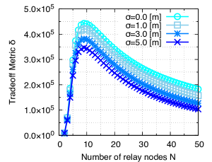
Figure 13: Effect of localization uncertainty on the tradeoff metric $\delta$.

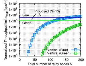
Figure 14: Comparison of the proposed SOWN with a conventional vertical UOWN ($N_{L}=5$).

Figure 15: A two-dimensional SOWN with $N_{\mathrm{L}}=4$ and $N_{\mathrm{H}}=3$.    Figure 16: Comparison of the optimal and constant relay intervals in the two-dimensional case ($N_{\mathrm{L}}=6$).

5.2 Extension to a two-dimensional SOWN

The optimization procedure we have developed can be extended to a two-dimensional SOWN as follows. Suppose that a two-dimensional area $\mathcal{L}\times\mathcal{H}\subset\mathbb{R}^{2}$ of a seafloor is covered by $N$ relay nodes, where $\mathcal{L}=[0,L]$ as before and $\mathcal{H}:=[0,H]$ ($H>0$). We assume that the sink node is placed at the origin $(0,0)$ and relay nodes are to be placed in a grid with non-constant spacings; the $i$th spacing along the $x$-axis is denoted by $\ell_{i}$ and the $j$th spacing along the $y$-axis is denoted by $h_{j}$. See Fig. 16 for an illustration. Let $N_{\mathrm{L}}$ (resp. $N_{\mathrm{L}}$) denote the number of nodes placed along the $x$-axis (resp. $y$-axis) for each row (resp. column). Note that the total number of relay nodes in the network (excluding the sink node) is given by $N=N_{\mathrm{L}}N_{\mathrm{H}}-1$. Hereafter we refer to the node placed at the $i$th column ($i=0,1,\ldots,N_{\mathrm{L}}-1$) and the $j$th row ($j=0,1,\ldots,N_{\mathrm{H}}-1$) as the ($i,j$)th node, where the $(0,0)$th node denotes the sink node. By definition, the position $(x_{i},y_{i})$ of the ($i,j$)th node is written as $(x_{i},y_{i})=(\sum_{k=1}^{i}\ell_{k},\sum_{k^{\prime}=1}^{j}h_{k^{\prime}})$. Similarly to the one-dimensional case, we assume that generation times of data packets follow a general point process with intensity $\lambda$, and the generation points of those packets are distributed uniformly on $\mathcal{L}\times\mathcal{H}$. The normalized traffic load $q$ is then defined as (cf. (2))

$$q=\frac{\lambda B}{LH},$$ (21)

where $B$ denotes the mean data size as before. Each packet is collected by the node nearest from its generation point and delivered to the sink node with multi-hop transmission. The cover area $\mathcal{C}_{i,j}$ of the ($i,j$)th node is then its two-dimensional Voronoi cell, which is a rectangle as depicted in Fig. 16. Also, the traffic intensity $\rho_{i,j}(q,\bm{x},\bm{y})$ of external arrivals to the ($i,j$)th node is given by $\rho_{i,j}(q,\bm{x},\bm{y})=q|\mathcal{C}_{i,j}|$; note here that cover areas $\mathcal{C}_{i,j}$ are, by definition, determined by the node placement ($\bm{x},\bm{y}$).

To formulate an optimal relay placement problem in the two-dimensional case, we have to specify the routing paths. Here we concentrate on the basic routing policy shown in Fig. 16: each packet is first transmitted along the $x$-axis to the left-most node and then transmitted along the $y$-axis to the sink node. In this setting, the one-dimensional optimal relay placement problem (U) maximizing the normalized throughput limit $q_{\sup}$ readily extends to the two-dimensional case:

$$\underset{q\in\mathbb{R},\,\bm{\ell}\in\mathbb{R}^{N_{\mathrm{L}}-1},\,\bm{h}\in\mathbb{R}^{N_{\mathrm{H}}-1},\,}{\mathrm{maximize}}\;\;q$$

$$\hskip 20.00003pt\mathrm{s.t.} R(\ell_{i})-\max_{j\in\mathcal{N}_{\mathrm{H}}}\left(\frac{h_{j}+h_{j+1}}{2}\right)\left(\frac{q\ell_{i}}{2}-\sum_{n=i+1}^{N}q\ell_{n}\right)\geq 0,\quad i\in\mathcal{N}_{\mathrm{L}},$$

$$R(h_{j})-L\left(\frac{qh_{j}}{2}-\sum_{n=j+1}^{N}qh_{n}\right)\geq 0,\;\;j\in\mathcal{N}_{\mathrm{L}},$$

$$q\geq 0,\;\;\sum_{i=1}^{N_{\mathrm{L}}}\ell_{i}=L,\;\;\sum_{j=1}^{N_{\mathrm{H}}}h_{j}=H,\;\;\ell_{i}\geq 0,\,i\in\mathcal{N}_{\mathrm{L}},\;\;h_{j}\geq 0,\,j\in\mathcal{N}_{\mathrm{H}}, \mbox{U}_{\mathrm{2D}}$$ ()

where $\mathcal{N}_{\mathrm{L}}:=\{1,2,\ldots,N_{\mathrm{L}}-1\}$, $\mathcal{N}_{\mathrm{H}}:=\{1,2,\ldots,N_{\mathrm{H}}-1\}$, and $h_{N_{\mathrm{H}}}:=0$.

Observe that for a fixed spacings $\bm{\ell}$ (resp. $\bm{h}$) along the $x$-axis (resp. $y$-axis), the optimization problem ($\mbox{U}_{\mathrm{2D}}$) reduces to the one-dimensional problem (U) by replacing $R(\cdot)$ with $R(\cdot)/L$ (resp. $R(\cdot)/\max_{j\in N_{\mathrm{H}}}((h_{j}+h_{j+1})/2)$). Assuming that communication links along the $y$-axis become bottlenecks of the system (we shall shortly come back to this point), we thus obtain optimal spacings $(\bm{\ell}^{*},\bm{h}^{*})$ by first solving (U) with $R(\cdot)$ replaced by $R(\cdot)/L$ to obtain $\bm{h}^{*}$ and then solving (U) with $R(\cdot)$ replaced by $R(\cdot)/\max_{j\in N_{\mathrm{H}}}((h_{j}^{*}+h_{j+1}^{*})/2)$ to obtain $\bm{\ell}^{*}$. Write the optimal value obtained at the first step as $q_{y}^{*}\cdot L$ and that obtained at the second step as $q_{x}^{*}\cdot\max_{j\in N_{\mathrm{H}}}(h_{j}^{*}+h_{j+1}^{*})/2$. The achieved objective value is then given by $\min(q_{x}^{*},q_{y}^{*})$, as it is the maximum $q$ satisfying all the constraints. That is, we can ensure that the above-mentioned assumption (communication links along the $y$-axis are bottlenecks) is indeed satisfied by checking if $q_{y}^{*}<q_{x}^{*}$ is satisfied. Because $q_{x}^{*}$ increases with $N_{L}$, we can find the minimum $N_{L}$ such that $q_{y}^{*}<q_{x}^{*}$ holds, and in that case, the maximum normalized throughput limit $q_{\sup}^{*}$ (i.e., the optimal value of ($\mbox{U}_{\mathrm{2D}}$)) is given by $q_{\sup}^{*}=q_{y}^{*}$. Therefore, the above procedure gives the optimal (i.e., the minimum) number of nodes $N_{L}$ along the $x$ axis as well as the optimal spacings $(\bm{\ell}^{*},\bm{h}^{*})$ of relay nodes.

Similarly to the one-dimensional case, we define the tradeoff metric $\delta:=q_{\sup}/N$. Fig. 16 compares the optimal relay placement with the constant placement $\bm{l}=(L/N_{\mathrm{L}},L/N_{\mathrm{L}},\ldots,L/N_{\mathrm{L}})$, $\bm{h}=(H/N_{\mathrm{H}},H/N_{\mathrm{H}},\ldots,H/N_{\mathrm{H}})$ for $N_{\mathrm{L}}=6$ and the blue light with the parameter values in Table 1. We observe that the optimal relay placement developed in this paper provides significant performance improvement also in the two-dimensional network.

6 Conclusions

In this paper, we considered an optimal relay placement problem for a one-dimensional SOWN. We modeled such a network as a queueing network with a general input process and we formulated the relay placement problem whose objective is to maximize the stability region of the whole system. We showed that this problem has a non-convex feasible region, whose global optimization is generally a difficult task. We then developed an algorithm (presented in Algorithm 1) to efficiently compute a globally optimal solution and investigated the mathematical structure of the obtained optimal solution. Through numerical evaluations, we showed that the obtained optimal solution provides a significant performance gain, compared to the conventional constant-interval relay placement. We further proposed a method to determine a reasonable number of relay nodes by introducing the tradeoff metric $\delta$, defined as the achieved system performance per relay node. We also presented extensive numerical experiments, where the proposed method is compared with a conventional vertical relay, and discussions on several practical aspects of UOWC channels, such as the misalignment, the FOV, and the uncertainty in node placement, are given.

We finally demonstrated how to extend the developed optimal placement into a two-dimensional SOWN. While we focused on the case of regular-grid topology and a simple routing policy depicted in Fig. 16, there would be various possible other directions for extensions. For example, the mathematical result shown in Theorem 13 suggests that it is efficient to employ relay intervals $d_{N},d_{N-1},\ldots,d_{1}$ which decreases at least exponentially fast. Future works include an application of this insight to two-dimensional networks with more flexible topologies and sophisticated routing mechanisms that enables us to deal with occurrences of node and link failure, which is the important aspect for the reliability of underwater networks as an infrastructure.

Appendix A Proof of Theorem 7

For ease of presentation, we introduce a slightly generalized problem. Let $g:[0,\infty)\to[-\infty,g(0))$ denote a convex function with $g(0)>0$ which is strictly decreasing and continuously differentiable. For $k=1,2,\ldots$, we define $f_{i}^{(k)}(\bm{y})$ ($\bm{y}\in\mathbb{R}^{k}$, $\bm{y}\geq\bm{0}$) as

$$f_{i}^{(k)}(\bm{y})=g(y_{i})-\sum_{n=1}^{i-1}y_{n},\;\;i=1,2,\ldots,k.$$ (22)

Let $\bm{f}^{(k)}(\bm{y}):=(f_{1}^{(k)}(\bm{y}),f_{2}^{(k)}(\bm{y}),\ldots,f_{k}^{(k)}(\bm{y}))^{\top}$ and $u^{(k)}(\bm{y}):=\sum_{i=1}^{k}y_{i}$. We consider the following optimization problem for $k=1,2,\ldots$:

$$\underset{\bm{y}\in\mathbb{R}^{k}}{\mathrm{maximize}}\;u^{(k)}(\bm{y})\quad\mathrm{s.t.}\;\bm{f}^{(k)}(\bm{y})\geq\bm{0},\,\bm{y}\geq\bm{0}. \mbox{P}^{(k)}$$ ()

Since $f_{i}^{(k)}$ and $u^{(k)}$ are both convex, ($\mbox{P}^{(k)}$) belongs to RCP. We can readily verify that ($\mbox{P}^{(N)}$) reduces to (S_q), letting $d_{n}=y_{N-n+1}$ ($n=1,2,\ldots,N$) and $g(x)=g_{q}(x)$ ($x\geq 0$).

Let $g^{-1}:(-\infty,g(0)]\to[0,\infty)$ denote the inverse function of $g$. Because $g$ is assumed to be convex and strictly decreasing, $g^{-1}$ is also convex and strictly decreasing. Note that

$$g^{-1}(g(0))=0,\quad g^{-1}(z)>0,\;\;-\infty<z<g(0).$$ (23)

Below we provide a proof of the following lemma, which readily implies Theorem 7:

Lemma 14.

• If $g^{-1}(0)\geq g(0)$, then the following $\bm{y}^{*}$ is an optimal solution of ($\mbox{P}^{(k)}$)

  $$\bm{y}^{*}=(g^{-1}(0),0,0,\ldots,0)^{\top}\in\mathbb{R}^{k},$$ (24)

• If $g^{-1}(0)<g(0)$, a recursion

  $$y_{1}^{*} =g^{-1}(0),\quad y_{i}^{*}=g^{-1}\left(\sum_{j=1}^{i-1}y_{j}^{*}\right),\;\;i=2,3,\ldots,$$ (25)

  well defines a sequence $\{y_{i}^{*}\}_{i=1,2,\ldots}^{*}$ such that

  $$0<y_{i+1}^{*}<y_{i}^{*},\quad i=1,2,\ldots,$$ (26)

  and for $k=1,2,\ldots$, the following $\bm{y}^{*}$ is an optimal solution of ($\mbox{P}^{(k)}$).

  $$\bm{y}^{*}=(y_{1}^{*},y_{2}^{*},\ldots,y_{k}^{*})^{\top}\in\mathbb{R}^{k}.$$ (27)

We start with considering the number of zeros that an optimal solution can have (see Remark 8). Let $\mathcal{A}^{(k)}\subseteq\mathbb{R}^{k}$ denote the set of feasible solutions of ($\mbox{P}^{(k)}$), and let $\mathcal{Y}^{(k)}\subseteq\mathcal{A}^{(k)}$ denote the set of optimal solutions. For $\bm{y}\in\mathbb{R}^{k}$, we define $\kappa(\bm{y})$ as the number of elements of $\bm{y}$ which are equal to zero. We define $\phi^{(k)}$ as the maximum number of zeros in an optimal solution of ($\mbox{P}^{(k)}$):

$$\phi^{(k)}=\max\{\kappa(\bm{y});\,\bm{y}\in\mathcal{Y}^{(k)}\}.$$ (28)

Lemma 15.

For $k=1,2,\ldots$, the optimal value of ($\mbox{P}^{(k)}$) is equal to that of ($\mbox{P}^{(k-\phi^{(k)})}$):

$$\max\{u^{(k)}(\bm{y});\,\bm{y}\in\mathcal{A}^{(k)}\}=\max\{u^{(k-\phi^{(k)})}(\bm{y});\,\bm{y}\in\mathcal{A}^{(k-\phi^{(k)})}\}.$$ (29)

Proof.

Since the case of $\phi^{(k)}=0$ is trivial, we assume $\phi^{(k)}>0$. For any $\bm{y}\in\mathbb{R}^{k}$, let $y_{+,i}$ denote the $i$th non-zero element of $\bm{y}$. Let $\mathcal{Y}_{+}^{(k)}:=\{(y_{+,1},y_{+,2},\ldots,y_{+,k-\phi^{(k)}})^{\top};\,\kappa(\bm{y})=\phi^{(k)},\bm{y}\in\mathcal{Y}^{(k)}\}.$ It is readily verified that $\mathcal{Y}_{+}^{(k)}\subseteq\mathcal{A}^{(k-\phi^{(k)})}$, and therefore $\max\{u^{(k)}(\bm{y});\,\bm{y}\in\mathcal{A}^{(k)}\}=\max\{u^{(k-\phi^{(k)})}(\bm{y});\,\bm{y}\in\mathcal{Y}_{+}^{(k)}\}\leq\max\{u^{(k-\phi^{(k)})}(\bm{y});\,\bm{y}\in\mathcal{A}^{(k-\phi^{(k)})}\}.$ We then obtain Lemma 15 because $\max\{u^{(k-\phi^{(k)})}(\bm{y});\,\bm{y}\in\mathcal{A}^{(k-\phi^{(k)})}\}\leq\max\{u^{(k)}(\bm{y});\,\bm{y}\in\mathcal{A}^{(k)}\}$ also follows from that $(\bar{\bm{y}},0,0,\ldots,0)^{\top}\in\mathbb{R}^{k}$ is a feasible solution of ($\mbox{P}^{(k)}$) for any $\bar{\bm{y}}\in\mathcal{Y}^{(k-\phi^{(k)})}$. ∎

Corollary 16.

$\phi^{(k-\phi^{(k)})}=0$ ($k=1,2,\ldots$).

Proof.

Because the case of $\phi^{(k)}=0$ is trivial, we assume $\phi^{(k)}>0$. If $\phi^{(k-\phi^{(k)})}>0$ holds, ($\mbox{P}^{(k-\phi^{(k)})}$) has an optimal solution $\hat{\bm{y}}\in\mathcal{Y}^{(k-\phi^{(k)})}$ such that $\kappa(\hat{\bm{y}})>0$. It then follows from Lemma 15 that $\hat{\bm{y}}_{\mathrm{e}}:=(\hat{\bm{y}},0,0,\ldots,0)^{\top}\in\mathbb{R}^{k}$ is an optimal solution of ($\mbox{P}^{(k)}$). This implies $\kappa(\hat{\bm{y}}_{e})=\kappa(\hat{\bm{y}})+\phi^{(k)}>\phi^{(k)}$, which contradicts the definition (28) of $\phi^{(k)}$. ∎

We can verify that $\nabla\bm{f}^{(k)}(\bm{y})$ is a lower-triangular matrix with non-zero (negative) diagonal elements. We thus have $\det(\nabla\bm{f}^{(k)}(\bm{y}))\neq 0$, so that $\mathrm{rank}(\nabla\bm{f}^{(k)}(\bm{y}))=k$. Therefore, if $\bar{\bm{y}}\in\mathbb{R}^{k}$ satisfies $\bm{f}^{(k)}(\bar{\bm{y}})=\bm{0}$ and $\bar{\bm{y}}\geq\bm{0}$, then it is a basic solution of ($\mbox{P}^{(k)}$). Furthermore, the following Lemma 17 immediately follows from Remark 6:

Lemma 17.

If $\bar{\bm{y}}\in\mathbb{R}^{k}$ is a basic solution of ($\mbox{P}^{(k)}$) satisfying $\bar{\bm{y}}>\bm{0}$, then $\bm{f}^{(k)}(\bar{\bm{y}})=\bm{0}$ holds.

Lemma 18.

For fixed $k$ ($k=1,2,\ldots$), the followings hold:

• If there exists no vector $\bar{\bm{y}}\in\mathbb{R}^{k}$ satisfying $\bm{\bar{\bm{y}}}>\bm{0}$ and $\bm{f}^{(k)}(\bar{\bm{y}})=\bm{0}$, then $\phi^{(k)}>0$.

• If $\phi^{(k)}=0$, then ($\mbox{P}^{(k)}$) has an optimal solution $\bar{\bm{y}}\in\mathbb{R}^{(k)}$ satisfying $\bar{\bm{y}}>\bm{0}$ and $\bm{f}^{(k)}(\bar{\bm{y}})=\bm{0}$.

Proof.

We first consider (ii). When $\phi^{(k)}=0$, the elements of each optimal solution of ($\mbox{P}^{(k)}$) are all positive. It then follows from Lemma 5 that ($\mbox{P}^{(k)}$) has an optimal solution $\bar{\bm{y}}>\bm{0}$ which is also basic. Therefore, we have $\bm{f}(\bar{\bm{y}})=\bm{0}$ from Lemma 17, which proves (ii).

We next consider (i). The contraposition of (ii) is that if there exists no optimal solution $\bar{\bm{y}}$ of ($\mbox{P}^{(k)}$) satisfying $\bm{\bar{\bm{y}}}>\bm{0}$ and $\bm{f}^{(k)}(\bar{\bm{y}})=\bm{0}$, then $\phi^{(k)}>0$. We thus have (i) from $\mathcal{Y}^{(k)}\subseteq\mathbb{R}^{k}$. ∎

We can readily verify that if $\{y_{i}^{*}\}_{i=1,2,\ldots}$ in (25) is well-defined, $\bm{y}=(y_{1}^{*},y_{2}^{*},\ldots,y_{k}^{*})^{\top}$ is the unique solution of $\bm{f}^{(k)}(\bm{y})=0$. Note that $y_{1}^{*}$ is always well defined, while $y_{i}^{*}$ ($i=1,2,\ldots$) is not well-defined if $\sum_{j=1}^{i-1}y_{i}^{*}>g(0)$ because the domain of $g^{-1}$ is $(-\infty,g(0)]$. We then define $N^{*}\in\{2,3,\ldots\}\cup\{\infty\}$ as

$$N^{*}=\sup\left\{i\in\{2,3,\ldots\};\,\sum_{j=1}^{i-2}y_{j}^{*}<g(0)\right\}.$$ (30)

By definition $y_{i}^{*}$ is well-defined at least for $1\leq i<N^{*}$. In addition, if $N^{*}<\infty$, then $\sum_{j=1}^{N^{*}-1}y_{j}^{*}\geq g(0)$, so that $g^{-1}(\sum_{j=1}^{N^{*}-1}y_{j}^{*})$ is either equal to zero or not well-defined. We thus have

$$y_{i}^{*}>0,\quad 1\leq i<N^{*}.$$ (31)

Furthermore, because $g^{-1}$ is a strictly decreasing function,

$$y_{i}^{*}<y_{i-1}^{*},\quad 1\leq i<N^{*}.$$ (32)

Let $\{z_{i}^{*}\}_{1\leq i<N^{*}}$ denote a sequence of non-negative numbers defined as

$$z_{0}^{*}=0,\quad z_{i}^{*}=\sum_{j=1}^{i}y_{j}^{*},\;\;1\leq i<N^{*},$$ (33)

for which we have from (31),

$$z_{i}^{*}<z_{i+1}^{*},\quad 0\leq i<N^{*}.$$ (34)

Additionally, because (25) and (33) imply

$$y_{i}^{*} =z_{i}^{*}-z_{i-1}^{*},\qquad 1\leq i<N^{*},$$ (35)

$$y_{i}^{*} =g^{-1}(z_{i-1}^{*}),\qquad 1\leq i<N^{*},$$ (36)

$z_{i}^{*}$ satisfies the following recursion:

$$z_{0}^{*}=0,\quad z_{i}^{*}=z_{i-1}^{*}+g^{-1}(z_{i-1}^{*}),\;\;1\leq i<N^{*}.$$ (37)

With defining a function $h:(-\infty,g(0)]\rightarrow\mathbb{R}$ as

$$h(z)=z+g^{-1}(z),\;\;-\infty<z\leq g(0),$$ (38)

we rewrite (37) as

$$z_{0}^{*}=0,\quad z_{i}^{*}=h(z_{i-1}^{*}),\;\;1\leq i<N^{*}.$$ (39)

It is readily verified from (23) and the definition of $h$ that

$$h(z) >z,\;\;-\infty<z<g(0),$$ (40)

$$h(g(0)) =g(0).$$ (41)

Lemma 19.

Either $N^{*}=2$ or $N^{*}=\infty$ holds. Specifically, if $g^{-1}(0)\geq g(0)$, then $N^{*}=2$, and otherwise $N^{*}=\infty$.

Proof.

Because $g^{-1}(0)\geq g(0)\Rightarrow N^{*}=2$ immediately follows from the definitions of $y_{i}^{*}$ and $N^{*}$, we consider the case of $g^{-1}(0)<g(0)$ below. We first show that

$$g^{-1}(0)<g(0)\ \Rightarrow\ g^{\prime}(0)<-1.$$ (42)

Since $g$ is assumed to be a convex function, its derivative $g^{\prime}$ is a non-decreasing function. It then follows that if $g^{\prime}(0)\geq-1$, then $g^{\prime}(y)\geq-1\;\mbox{for $y\geq 0$}$, so that

$$y_{1}^{*}=\int_{0}^{g^{-1}(0)}\mathrm{d}y\geq\int_{0}^{g^{-1}(0)}(-g^{\prime}(y))\mathrm{d}y=g(0),$$ (43)

i.e., $g^{\prime}(0)\geq-1\ \Rightarrow\ y_{1}^{*}\geq g(0)$. We thus obtain (42), taking the contraposition.

Below, we proceed by considering two exclusive cases, under the assumption $g^{-1}(0)<g(0)$.

Case 1. $(g^{-1})^{\prime}(0)>-1$: Because $g^{-1}:(-\infty,g(0)]\rightarrow[0,\infty)$ is a convex function as noted above, its derivative $(g^{-1})^{\prime}$ is a non-decreasing function, so that we have from $(g^{-1})^{\prime}(0)>-1$,

$$(g^{-1})^{\prime}(z)>-1,\quad 0\leq z\leq g(0).$$ (44)

It then follows from (38) that $h$ is a strictly increasing function. Furthermore, we obtain from $g^{-1}(z)>0$ ($-\infty\leq z<g(0)$) and (41),

$$0<h(z)<g(0),\;\;0\leq z<g(0).$$ (45)

We then have $N^{*}=\infty$ from the following relation obtained by the induction with (39) and (45):

$$0<z_{i}^{*}<g(0),\quad i=1,2,\ldots.$$ (46)

Case 2. $(g^{-1})^{\prime}(0)\leq-1$: From (42) and $(g^{-1})^{\prime}(g(0))=1/g^{\prime}(0)$, we have (cf. (44))

$$(g^{-1})^{\prime}(g(0))>-1.$$ (47)

Recall that $g$ is assumed to be continuously differentiable, so that $(g^{-1})^{\prime}(y)$ is a continuous function. We can then verify that there exists $\beta\in[0,g(0))$ satisfying $(g^{-1})^{\prime}(\beta)=-1$, using $(g^{-1})^{\prime}(0)\leq-1$ and the intermediate value theorem. Note that such $\beta$ is not necessarily unique, because $(g^{-1})^{\prime}$ is not necessarily strictly increasing. Instead, the set of such $\beta$ is bounded above, so that its maximum value $\beta^{*}$ is uniquely obtained:

$$\beta^{*}=\max\{\beta\in[0,g(0));\,(g^{-1})^{\prime}(\beta)=-1\}.$$ (48)

It is then readily verified that

$$(g^{-1})^{\prime}(z) \leq-1,\qquad 0\leq z\leq\beta^{*},$$ (49)

$$(g^{-1})^{\prime}(z) >-1,\qquad\beta^{*}<z\leq g(0).$$ (50)

We have from (49),

$$\beta^{*}=\int_{0}^{\beta^{*}}\mathrm{d}z \leq\int_{0}^{\beta^{*}}(-1)\cdot(g^{-1})^{\prime}(z)\mathrm{d}z=g^{-1}(0)-g^{-1}(\beta^{*})<g^{-1}(0),$$ (51)

so that (37) and $g^{-1}(0)<g(0)$ imply

$$\beta^{*}<z_{1}^{*}=g^{-1}(0)<g(0).$$ (52)

It follows from (38) and (50) that $h(z)$ is strictly increasing for $\beta^{*}<z\leq g(0)$. Furthermore, (40) implies $h(\beta^{*})>\beta^{*}$. We can then verify that (cf. (45)):

$$\beta^{*}<h(z)<g(0),\qquad\beta^{*}\leq z<g(0).$$ (53)

We then obtain $N^{*}=\infty$ because the induction using (52) and (53) yields

$$\beta^{*}<z_{i}^{*}<g(0),\quad i=1,2,\ldots.\qed$$ (54)

Lemma 20.

For $k=2,3,\ldots$, the followings hold:

• If $g^{-1}(0)\geq g(0)$, there exists no vector $\bar{\bm{y}}\in\mathbb{R}^{k}$ such that $\bm{f}^{(k)}(\bar{\bm{y}})=\bm{0}$ and $\bar{\bm{y}}>\bm{0}$.

• If $g^{-1}(0)<g(0)$, $\bar{\bm{y}}=(y_{1}^{*},y_{2}^{*},\ldots,y_{k}^{*})^{\top}$ is the unique solution of $\bm{f}^{(k)}(\bar{\bm{y}})=\bm{0}$ and $\bar{\bm{y}}>\bm{0}$.

Proof.

Lemma 20 immediately follows from (22), (25), Lemma 19, and the definition of $N^{*}$. ∎

We are now in a position to prove Lemma 14.

Proof of Lemma 14.

We first consider the case of $g^{-1}(0)\geq g(0)$. In this case, we have $\phi^{(k)}>0$ for $k=2,3,\ldots$ from Lemma 18 (i) and Lemma 20 (i). Note that $y_{1}=g^{-1}(0)$ is the optimal solution of ($\mbox{P}^{(1)}$), and its optimal value is also equal to $g^{-1}(0)$. Obviously, we have $\phi^{(2)}=1$, so that the optimal value of ($\mbox{P}^{(2)}$) equals to $g^{-1}(0)$. Owing to Lemma 15, the optimal value of ($\mbox{P}^{(3)}$) is then equal to $g^{-1}(0)$, which implies $\phi^{(3)}=2$. Therefore, proceeding in the same way, we can readily show that $\phi^{(k)}=k-1$ and the optimal value of $(\mbox{P}^{(k)})$ is equal to $g^{-1}(0)$ for $k=2,3,\ldots$. Because (24) achieves the optimal value $g^{-1}(0)$ of $(\mbox{P}^{(k)})$, we obtain Lemma 14 (i).

We next consider the case of $g^{-1}(0)<g(0)$. Note first that the well-definedness of $\{y_{i}\}_{i=1,2,\ldots}^{*}$ and (26) have been proved in (31), (32), and Lemma 19. It then follows from Lemma 20 (ii) that $(y_{1}^{*},y_{2}^{*},\ldots,y_{k-\phi^{(k)}}^{*})^{\top}\in\mathbb{R}^{k}$ is the unique solution of $\bm{f}^{(k-\phi^{(k)})}(\bar{\bm{y}})=\bm{0}$ and $\bar{\bm{y}}>\bm{0}$. Therefore, from Corollary 16 and Lemma 18 (ii), we can verify that $(y_{1}^{*},y_{2}^{*},\ldots,y_{k-\phi^{(k)}}^{*})^{\top}$ is an optimal solution of $(\mbox{P}^{(k-\phi^{(k)})})$ and that from Lemma 15, $\max\{u^{(k)}(\bm{y});\,\bm{y}\in\mathcal{A}^{(k)}\}=\sum_{i=1}^{k-\phi^{(k)}}y_{i}^{*}.$ Because $(y_{1}^{*},y_{2}^{*},\ldots,y_{k}^{*})^{\top}\in\mathcal{A}^{(k)}$, this equation implies $\sum_{i=1}^{k}y_{i}^{*}\leq\sum_{i=1}^{k-\phi^{(k)}}y_{i}^{*}$. Therefore, from (31) we have $\phi^{(k)}=0$, so that $(y_{1}^{*},y_{2}^{*},\ldots,y_{k}^{*})^{\top}$ is an optimal solution of $(\mbox{P}^{(k)})$. ∎

Appendix B Proof of Theorem 10

We first consider (a). Note first that Theorem 7 and Lemma 9 imply

$$x_{q,N}^{*}\geq g_{q}^{-1}(0),\quad 0<q<q_{0},\qquad x_{q,N}^{*}=g_{q}^{-1}(0),\quad q\geq q_{0},$$ (55)

so that we obtain $\lim_{q\to 0+}x_{q,N}^{*}\geq\lim_{q\to\infty}g_{q}^{-1}(0)=\infty,$ and $\lim_{q\to\infty}x_{q,N}^{*}=\lim_{q\to\infty}g_{q}^{-1}(0)=0.$

For $q\geq q_{0}$, we have from (55) that $x_{q,N}^{*}$ is continuous and strictly decreasing in $q$ (cf. (8)). We then assume $0<q<q_{0}$. Let $h_{q}:(-\infty,g_{q}(0)]\to\mathbb{R}$ be defined as (cf. (38))

$$h_{q}(s)=s+g_{q}^{-1}(s),\quad s>0.$$ (56)

We define $s_{q,i}$ ($i=1,2,\ldots,N$) as (cf. (33) and (39))

$$s_{q,1}=g_{q}^{-1}(0),\quad s_{q,i}=h_{q}(s_{i-1}),\;\;i=2,3,\ldots,N.$$ (57)

It is then readily verified from Theorem 7 that

$$x_{q,N}^{*}=s_{q,N},\quad 0<q<q_{0}.$$ (58)

$x_{q,N}^{*}$ is thus a continuous function of $q$. By definition, $s_{q,1}$ and $h_{q}(s)$ (for a fixed $s$) are strictly decreasing with respect to $q$ (cf. (8)). Furthermore, as shown in the proof of Lemma 19, for a fixed $q$, $h_{q}(s)$ is strictly increasing with respect to $s$ for $s_{q,1}=g_{q}^{-1}(0)<s\leq g_{q}(0)$. We can then show by induction that $s_{q,i}>s_{q^{\prime},i},$ ($i=1,2,\ldots,N$) for any $0<q<q^{\prime}<q_{0}$, which and (58) prove that $x_{q,N}^{*}$ is continuous and strictly decreasing for $0<q<q_{0}$.

What remains is to prove that $x_{q,N}^{*}$ is continuous at $q=q_{0}$. By definition of $q_{0}$, we have $\lim_{q\to q_{0}-}g_{q}^{-1}(0)=g_{q_{0}}(0)$, so that $\lim_{q\to q_{0}-}s_{q,i}=g_{q_{0}}(0)$ ($i=1,2,\ldots,N$). $x_{q,N}^{*}$ is thus continuous at $q=q_{0}$ because $\lim_{q\to q_{0}+}x_{q,N}^{*}=x_{q_{0}}^{*}=g_{q_{0}}^{-1}(0)=g_{q_{0}}(0).$

We then consider (b). We first show the following relations:

$$x_{q,N}^{*}>L\ \Rightarrow\ q<q_{\sup}^{*},\qquad x_{q,N}^{*} <L\ \Rightarrow\ q>q_{\sup}^{*}.$$ (59)

Suppose $x_{q,N}^{*}>L$ and define $\hat{q}:=qx_{q,N}^{*}/L$ and $\hat{d}_{i}:=d_{q,i}^{*}L/x_{q,N}^{*}$ ($i=1,2,\ldots,N$), where we have $\hat{q}>q$ and $\hat{d}_{i}\leq d_{q,i}^{*}$. It is then verified that $(\hat{q},\hat{d}_{1},\hat{d}_{2},\ldots,\hat{d}_{N})^{\top}$ is a feasible solution of (U), as $\sum_{i=1}^{N}\hat{d}_{i}=L$ and $R(\hat{d}_{i})\geq R(d_{q,i}^{*})$. We thus obtain $q_{\sup}^{*}\geq\hat{q}>q$ from the optimality of $q_{\sup}^{*}$, which proves the first relation in (59). On the other hand, the second relation follows from that

$$x_{q,N}^{*}<L\ \Rightarrow\ \mbox{ For any $\bm{d}\in\mathbb{R}^{N}$, $(q,\bm{d})$ is an infeasible solution of (\ref{opt:original}), }$$ (60)

which is proved by contradiction: if there exists $\bm{d}\in\mathbb{R}^{N}$ such that $(q,\bm{d})$ is a feasible solution of (U), $\bm{d}$ is also a feasible solution of (S_q) satisfying $\sum_{i=1}^{N}d_{i}=L$, contradicting $x_{q,N}^{*}<L$.

Taking the contrapositions of (59), we have $q\geq q_{\sup}^{*}\Rightarrow x_{q,N}^{*}\leq L$ and $q\leq q_{\sup}^{*}\Rightarrow x_{q,N}^{*}\geq L$, which implies $q=q_{\sup}^{*}\Rightarrow x_{q,N}^{*}=L$. Owing to Theorem 10 (a), this also implies $x_{q,N}^{*}=L\Rightarrow q=q_{\sup}^{*}$, so that we obtain the last equivalence relation in (17). Furthermore, $(q_{\sup}^{*},\bm{d}_{q_{\sup}^{*}}^{*})$ is an optimal solution of (U) because it is a feasible solution with the optimal objective value $q_{\sup}^{*}$.

Finally, the first and second equivalence relations in (17) are immediately obtained, noting that Theorem 10 (a) and the last relation in (17) imply $q<q_{\sup}^{*}\Leftrightarrow x_{q,N}^{*}>x_{q_{\sup}^{*},N}^{*}=L$ and $q>q_{\sup}^{*}\Leftrightarrow x_{q,N}^{*}<x_{q_{\sup}^{*},N}^{*}=L$. ∎

Appendix C Proof of Theorem 13

We consider the slightly generalized problem ($\mbox{P}^{(k)}$) considered in Appendix A, assuming $g^{-1}(0)<g(0)$. It is sufficient to show that under this assumption,

$$\gamma:=1+\frac{1}{g^{\prime}(0)}\in(0,1),$$ (61)

and that $y_{i}^{*}$ defined in (25) satisfies the followings: if $(g^{-1})^{\prime}(0)>-1$, then

$$0<y_{i}^{*}\leq\gamma^{i-1}g^{-1}(0),\;\;i=1,2,\ldots,$$ (62)

and otherwise

$$0<y_{i}^{*}\leq\gamma^{i-2}g^{-1}(g^{-1}(0)),\;\;i=2,3,\ldots.$$ (63)

Because (61) immediately follows from (42), we show (62) and (63) below.

We first consider the case $(g^{-1})^{\prime}(0)>-1$. As shown in the proof of Lemma 19, $h(z)$ ($0\leq z\leq g(0)$) is a strictly increasing function in this case. In addition, we have $(g^{-1})^{\prime}(z)\leq(g^{-1})^{\prime}(g(0))$ ($0\leq z\leq g(0)$) because $g^{-1}(z)$ is a convex function. We then have for any $0\leq t_{1}\leq t_{2}\leq g(0)$,

$$|h(t_{2})-h(t_{1})| =t_{2}-t_{1}+g^{-1}(t_{2})-g^{-1}(t_{1})$$

$$=t_{2}-t_{1}+\int_{t_{1}}^{t_{2}}(g^{-1})^{\prime}(t)\mathrm{d}t\leq t_{2}-t_{1}+(g^{-1})^{\prime}(g(0))\int_{t_{1}}^{t_{2}}\mathrm{d}t=\gamma|t_{2}-t_{1}|.$$ (64)

Furthermore, it follows from (41) and (45) that $0\leq h(z)\leq g(0)$ ($0\leq h(z)\leq g(0)$). Therefore, we can verify from (39) and Banach fixed point theorem that $\{z_{i}^{*}\}_{i=0,1,\ldots}$ converges to the unique fixed point of $h(z)$ ($0\leq z\leq g(0)$) given by $z=g(0)$. In addition, we have from (34) and (64),

$$y_{i+1}^{*} =z_{i+1}^{*}-z_{i}^{*}=h(z_{i}^{*})-h(z_{i-1}^{*})\leq\gamma(z_{i}^{*}-z_{i-1}^{*})=\gamma y_{i}^{*},\qquad i=1,2,\ldots$$ (65)

so that (62) is obtained by induction using $y_{1}^{*}=g^{-1}(0)$.

We next consider the case $(g^{-1})^{\prime}(0)\leq-1$. As shown in the proof of Lemma 19, $h(z)$ is strictly increasing for $\beta^{*}\leq z\leq g(0)$, where $\beta^{*}$ is defined in (48). We can then show in the same way as (64) that for any $\beta^{*}\leq t_{1}\leq t_{2}\leq g(0)$,

$$|h(t_{2})-h(t_{1})|\leq\gamma|t_{2}-t_{1}|.$$ (66)

Also, we have $\beta^{*}\leq h(z)\leq g(0)$ ($\beta^{*}\leq z\leq g(0)$) from (41) and (53). It thus follows from (52) and Banach fixed point theorem that $\{z_{i}^{*}\}_{i=0,1,\ldots}$ converges to the unique fixed point $z=g(0)$ of $h(z)$ in $\beta^{*}\leq z\leq g(0)$. Furthermore, in the same way as (65), we have $y_{i+1}^{*}\leq\gamma y_{i}^{*}$ ($i=2,3,\ldots$) from (34) and (66), so that we obtain (63) noting that $y_{2}^{*}=g^{-1}(g^{-1}(0))$ (see (25)). ∎

References

- [1] E. Felemban, F. K. Shaikh, U. M. Qureshi, A. A. Sheikh, and S. B.Qaisar, “Underwater sensor network applications: A comprehensive survey,” Int. J. of Distrib. Sens. Netw., vol. 11, no. 11, 2015.
- [2] I. F. Akyildiz, D. Pompili, and T. Melodia, “Underwater acoustic sensor networks: research challenges,” Ad Hoc Netw., vol. 3, no. 3, pp. 257–279, 2005.
- [3] H. Kaushal and G. Kaddoum, “Underwater optical wireless communication,” IEEE Access, vol. 4, pp. 1518–1547, 2016.
- [4] Z. Zeng, S. Fu, H. Zhang, Y. Dong, and J. Cheng, “A survey of underwater optical wireless communications,” IEEE Commun. Surv. Tutor., vol. 19, no. 1, pp. 204–238, 2017.
- [5] A. Celik, N. Saeed, B. Shihada, T. Y. Al-Naffouri, and M. Alouini, “End-to-end performance analysis of underwater optical wireless relaying and routing techniques under location uncertainty,” IEEE Trans. Wireless Commun., vol. 19, no. 2, pp. 1167–1181, 2020.
- [6] A. Celik, N. Saeed, B. Shihada, T. Y. Al-Naffouri, and M. Alouini, “SectOR: Sector-Based Opportunistic Routing Protocol for Underwater Optical Wireless Networks,” Proc. of 2019 IEEE WCNC, 2019.
- [7] N. Saeed, A. Celik, T. Y. Al-Naffouri, and M.-S. Alouini, “Underwater optical wireless communications, networking, and localization: A survey”, Ad Hoc Netw., vol. 94, 101935, 2019.
- [8] N. Saeed, A. Celik, M. Alouini, and T. Y. Al-Naffouri, “Performance analysis of connectivity and localization in multi-hop underwater optical wireless sensor networks,” IEEE Trans. Mobile Comput., vol. 18, no. 11, pp. 2604–2615, 2019.
- [9] N. Saeed, A. Celik, T. Y. Al-Naffouri, and M. Alouini, “Localization of energy harvesting empowered underwater optical wireless sensor networks,” IEEE Trans. Wireless Commun, vol. 18, no. 5, pp. 2652–2663, 2019.
- [10] C. Kam, S. Kompella, G. D. Nguyen, A. Ephremides, and Z. Jiang, “Frequency selection and relay placement for energy efficiency in underwater acoustic networks,” IEEE J. of Ocean. Eng., vol. 39, no. 2, pp. 331–342, 2014.
- [11] F. A. de Souza, B. S. Chang, G. Brante, R. D. Souza, M. E. Pellenz, and F. Rosas, “Optimizing the number of hops and retransmissions for energy efficient multi-hop underwater acoustic communications,” IEEE Sens. J., vol. 16, no. 10, pp. 3927–3938, 2016.
- [12] L. Liu, M. Ma, C. Liu, and Y. Shu, “Optimal relay node placement and flow allocation in underwater acoustic sensor networks,” IEEE Trans. on Commun., vol. 65, no. 5, pp. 2141–2152, 2017.
- [13] G. Prasad, D. Mishra, and A. Hossain, “Joint optimal design for outage minimization in DF relay-assisted underwater acoustic networks,” IEEE Commun. Lett., vol. 22, no. 8, pp. 172-4-1727, 2018.
- [14] J. W. Giles and I. N. Bankman, “Underwater optical communications systems. Part 2: basic design considerations,” Proc. IEEE MILCOM 2005, pp. 1700–1705, 2005.
- [15] M. Doniec, M. Angermann, and D. Rus, “An end-to-end signal strength model for underwater optical communications,” IEEE J. Ocean. Eng., vol. 38, no. 4, pp. 743–757, 2013.
- [16] M. Elamassie, F. Miramirkhani, and M. Uysal, “Performance characterization of underwater visible light communication,” IEEE Trans. Commun. vol. 67, no. 1, pp. 543–552, 2019.
- [17] K. Nakamura, I. Mizukoshi and M. Hanawa, “Optical wireless transmission of 405 nm, 1.45 Gbit/s optical IM/DD-OFDM signals through a 4.8 m underwater channel,” Opt. Exp., vol. 23, no. 2, pp. 1558–1566, 2015.
- [18] H. M. Oubei, J. R. Duran, B. Jaujua, H-Y. Wang, C-T. Tsai, Y-C. Chi, T. K. Ng, H-C. Kuo, J-H. He, M-S. Alouini, G-R. Lin and B. S. Ooi, “4.8 Gbit/s 16-QAM-OFDM transmission based on compact 450-nm laser for underwater wireless optical communication,” Opt. Exp., vol. 23, no. 18, pp. 23302–23309, 2015.
- [19] A. A-Halafi, H. M. Oubei, B. S. Ooi, and B. Shihada, “Real-time video transmission over different underwater wireless optical channels using directly modulated 520 nm laser diode,” IEEE J. Opt. Commun. Netw., vol. 9, no. 10, pp. 826–832, Oct. 2017.
- [20] T. C. Wu, Y. C. Chi, H. Y. Wang, C. T. Tsai, and G. R. Lin, “Blue laser diode enables underwater communication at 12.4 Gbps,” Sci. Rep., vol. 7 40480, 2017.
- [21] T. Kodama, K. Arai, K. Nagata, K. Nakamura, and M. Hanawa, “Underwater wireless optical access network with OFDM/SBMA system: Concept and demonstration,” Proc. OECC/PSC 2019, 2019.
- [22] S. Tang, Y. Dong, and X. Zhang, “Impulse response modeling for underwater wireless optical communication links,” IEEE Trans. Commun., vol. 62, no. 1, pp. 226–234, 2014.
- [23] S. Jaruwatanadilok, “Underwater wireless optical communication channel modeling and performance evaluation using vector radiative transfer theory,” IEEE J. Sel. Areas Commun., vol. 26, no. 9, pp. 1620–1627, 2008.
- [24] H. Zhang and Y. Dong, “General stochastic channel model and performance evaluation for underwater wireless optical links,” IEEE Trans. Wireless Commun., vol. 15, no. 2, pp. 1162–1173, 2016.
- [25] F. Akhoundi, J. A. Salehi, and A. Tashakori, “Cellular underwater wireless optical CDMA network: Performance analysis and implementation concepts,” IEEE Trans. Commun., vol. 63, no. 3, pp. 882–891, 2015.
- [26] M. V. Jamali, F. Akhoundi, and J. A. Salehi, ”Performance characterization of relay-assisted wireless optical CDMA networks in turbulent underwater channel.” IEEE Tran. Wireless Commun., vol. 15, no. 6, pp. 4104–4116, 2016.
- [27] M. V. Jamali, A. Chizari, and J. A. Salehi, “Performance analysis of multi-hop underwater wireless optical communication systems,” IEEE Photon. Technol. Lett., vol. 29, no. 5, pp. 462–465, 2017.
- [28] A. Vavoulas, H. G. Sandalidis, and D. Varoutas, “Underwater optical wireless networks: A k-connectivity analysis,” IEEE J. Ocean. Eng., vol. 39, no. 4, pp. 801–809, 2014.
- [29] N. Saeed, T. Y. Al-Naffouri, and M. Alouini, “Outlier detection and optimal anchor placement for 3-D underwater optical wireless sensor network localization,” IEEE Trans. Commun., vol. 67, no. 1, pp. 611–622, 2019.
- [30] A. Al-Halafi, A. Alghadhban, and B. Shihada, “Queuing delay model for video transmission over multi-channel underwater wireless optical networks,” IEEE Access, vol. 7, pp. 10515–10522, 2019.
- [31] F. Xing, H. Yin, X. Ji, and V. C. M. Leung, “Joint relay selection and power allocation for underwater cooperative optical wireless networks,” IEEE Trans. Wireless Commun., vol. 19, no. 1, pp. 251–264, 2020.
- [32] F. Baccelli and P. Brémaud, Elements of Queueing Theory, 2nd ed., Springer, Berlin, 2003.
- [33] S. Arnon and D. Kedar, “Non-line-of-sight underwater optical wireless communication network,” J. Opt. Soc. Am. A, vol. 26, no. 3, pp. 530–539, 2009.
- [34] C. D. Mobley, Light and Water: Radiative Transfer in Natural Waters. Academic Press, San Diego, CA, 1994.
- [35] J. G. Andrews, F. Baccelli, and R. K. Ganti, “A tractable approach to coverage and rate in cellular networks,” IEEE Trans. Commun., vol. 59, no. 11, pp. 3122–3134, 2011.
- [36] D. Lavery, T. Gerard, S. Erkilinc, Z. Liu, L. Galdino, P. Bayvel, and R. I. Killey, “Opportunities for optical access network transceivers beyond OOK [invited],” IEEE/OSA J. Opt. Commun. Netw., vol. 11, no. 2, pp. A186–A195, 2019.
- [37] R. J. Hillestad and S. E. Jacobsen, “Reverse convex programming,” Appl. Math. Optim., vol. 6, 63–78, 1980.
- [38] U. Ueing, “A combinatorial method to compute a global solution of certain non-convex optimization problems”, Numerical Methods for Non-Linear Optimization, F. A. Lootsma (ed.), 223–230, Academic Press, New York, NY, 1972.
- [39] H. Tuy, “Convex programs with an additional reverse convex constraint,” J. Optim. Theory Appl. vol. 52, no. 3, pp. 463–486, 1987.
- [40] K. Moshirvaziri and M. A. Amouzegar, “A deep-cutting-plane technique for reverse convex optimization,” IEEE Trans. Sys. Man Cyber. B, vol. 41, no. 4, pp. 1054–1060, 2011.
- [41] R. C. Smith and K. S. Baker, “Optical properties of the clearest natural waters (200–800 nm),” Appl. Opt., vol. 20, no. 2, pp. 177–184, 1981.
- [42] G. Riccobene et al. “Deep seawater inherent optical properties in the Southern Ionian Sea,” Astropart. Phys., vol. 27, no. 1, pp. 1–9, 2007.