Change-point tests for the tail parameter of Long Memory Stochastic Volatility time series
Abstract
We consider a change-point test based on the Hill estimator to test for structural changes in the tail index of Long Memory Stochastic Volatility time series. In order to determine the asymptotic distribution of the corresponding test statistic, we prove a uniform reduction principle for the tail empirical process in a two-parameter Skorohod space. It is shown that such a process displays a dichotomous behavior according to an interplay between the Hurst parameter, i.e., a parameter characterizing the dependence in the data, and the tail index. Our theoretical results are accompanied by simulation studies and the analysis of financial time series with regard to structural changes in the tail index.
Keywords: stochastic volatility; long-range dependence; change-point tests; tail empirical process; heavy tails; chaining
1 Introduction and motivation
The tail behavior of the marginal distribution of time series is of major relevance for statistics in applied sciences such as econometrics and hydrology, where heavy-tailed data occurs frequently. More precisely, time series from finance such as the log returns of exchange rates and stock market indices display heavy tails; see Mandelbrot, (1963). Furthermore, drastic events like the financial crisis in 2008 substantiate the importance of studying time series models that underlie financial data. Against this background, the identification of changes in the tail behavior of data-generating stochastic processes, that result in an increase or decrease in the probability of extreme events, is of utmost interest. In particular, the analysis of the tail behavior of financial data may pave the way for a corresponding adjustment of risk management for capital investments and, therefore, prevent from huge capital losses. Indeed, there is empirical evidence that the tail behavior of financial time series may change over time: Quintos et al., (2001) identify changes in the tail of Asian stock market indices, Galbraith and Zernov, (2004) find evidence for changes in the tail behavior of returns on U.S. equities, and Werner and Upper, (2004) detect structural breaks in high-frequency data of Bund future returns.
1.1 Tail index estimation and change-point problem
Let , , be a stationary time series whose marginal tail distribution function is regularly varying with index , , i.e., , where is slowly varying at infinity. Since the tail behavior of , , is primarily determined by the value of the tail index , identifying a change in the tail of data-generating processes corresponds to testing for a change-point in this parameter.
In particular, this means that, given a set of observations with , , we aim at deciding on the testing problem with
| and | ||||
Test statistics that are designed for identifying structural changes in the tail index are naturally derived from an estimation of the tail index . For some general results on tail index estimation see Drees, 1998a and Drees, 1998b . In this article, we focus on two estimators that are motivated by the fact that for a random variable with tail index
When we are given a set of observations , an approximation of the unknown distribution of by its empirical analogue gives the following estimator for the tail index:
| (1) |
where , , is a sequence with and . Replacing the deterministic levels in the formula for by for some , , where are the order statistics of the sample , yields the Hill estimator
As the most popular estimator for the tail index, established in Hill, (1975), the Hill estimator has been widely studied in the literature. Its limiting distribution was obtained under various model assumptions, including linear processes (Resnick and Stărică, (1997)), -mixing processes (Drees, (2000)), and Long Memory Stochastic Volatility models (Kulik and Soulier, (2011)). The first article that establishes a theory for change-point tests that are based on the Hill estimator seems to be Quintos et al., (2001). While Quintos et al., (2001) consider independent, identically distributed observations, ARCH- and GARCH-type processes, Kim and Lee, (2011) and Kim and Lee, (2012) extend their results to -mixing processes and residual-based change-point tests for processes with heavy-tailed innovations. In contrast, we study change-point tests for the tail index of Long Memory Stochastic Volatility time series based on the two estimators and . In fact, our results are the first to consider the change-point problem for stochastic volatility models and time series with long-range dependence.
To motivate the design of test statistics for deciding on the change-point problem , we temporarily assume that the change-point location is known, i.e., for a given we consider the testing problem with
For this testing problem, change-point tests have been considered in Phillips et al., (1990) and Koedijk et al., (1990). In order to decide on , we compare an estimation of the tail index based on the observations to an estimation of the tail index based on the whole sample . This idea leads to studying the following test statistic
Under the assumption that the change-point location is unknown under the alternative, it seems natural to consider the statistic for every potential change-point location and to decide in favor of the alternative hypothesis if the maximum of its values exceeds a predefined threshold. As a result, a change-point test for the testing problem that rests upon the estimator defined by (1) bases test decisions on the values of the statistic
| (2) |
with and with the sequential version of defined by
| (3) |
Likewise, a test statistic based on the Hill estimator is given by
with the sequential version of defined by
In this context, the most comprehensive theory for change-point tests is presented in Hoga, (2017). The author considers a number of test statistics based on different tail index estimators and derives their asymptotic distributions under the assumption of -mixing data generating processes.
In the following, we derive the asymptotic distribution of both estimators, i.e., and , and the corresponding tests statistics, i.e., and , under the hypothesis of stationary time series data. For this purpose, we first prove a limit theorem for the tail empirical process of Long Memory Stochastic Volatility time series in two parameters. This limit theorem does not necessarily relate to the change-point context. It can therefore be considered of independent interest and, thus, as the main theoretical result of our work. Our theoretical results are accompanied by simulation studies. As an empirical application of our tests, we consider Standard & Poor’s 500 daily closing index covering the period from January 2008 to December 2008, the year of the financial crisis. We identify a change in the data at exactly one day after Lehman Brothers filed for bankruptcy protection, an event which is thought to have played a major role in the unfolding of the crisis in 2007 –- 2008.
1.2 Tail empirical process
In order to derive the limit distribution of the tail estimators and , parametrized in , and the corresponding test statistics and , it is crucial to note that
| (4) |
where
As a result, asymptotics of the considered statistics can be derived from a limit theorem for the two-parameter tail empirical process
| (5) |
where does not correspond to the mean of , but rather to the limit of that mean, i.e., to
| (6) |
Among others, the tail empirical process in one parameter, i.e., , , has previously been studied in Mason, (1988), Einmahl, (1990), and Einmahl, (1992) for independent, identically distributed observations, in Rootzén, (2009) for absolutely regular processes, and in Kulik and Soulier, (2011) for Long Memory Stochastic Volatility time series. For the latter, the convergence of the two-parameter tail empirical process will be discussed in Section 2.2.
1.3 Long Memory Stochastic Volatility model
A phenomenon that is often encountered in the context of financial time series corresponds to the observation that the observations seem to be uncorrelated, whereas their absolute values or higher moments tend to be highly correlated. Another characteristic of financial time series is the occurrence of heavy tails. In particular, the distribution of the considered data often exhibits tails that are heavier than those of a normal distribution. The previously described features of financial data can be covered by stochastic volatility models.
Stochastic volatility model
The Long Memory Stochastic Volatility model that is taken as a basis of the theoretical results established in this article can be considered as a generalization of stochastic volatility models considered, for example, in Taylor, (1986). Initially, this model had been introduced by Breidt et al., (1998) and, independently, by Harvey, (2002). An overview of stochastic volatility models with long-range dependence and their basic properties is given in Deo et al., (2006) and in Hurvich and Soulier, (2009).
Stochastic volatility time series , , are typically defined via
| (7) |
where , , is a sequence of independent, identically distributed random variables with mean , and , , is a Gaussian process, independent of , .
While these models are often restricted to modeling a relatively fast decay of dependence in , , the so-called Long Memory Stochastic Volatility model allows for long-range dependence. In what follows, we will specify a corresponding dependence structure for , .
Subordinated Gaussian processes
The rate of decay of the autocovariance function is crucial to the definition of long-range dependence in time series.
Definition 1.1.
A (second-order) stationary, real-valued time series , , is called long-range dependent if its autocovariance function satisfies
with for some slowly varying function . We refer to as long-range dependence (LRD) parameter; see Pipiras and Taqqu, (2017), p. 17.
We will focus our considerations on long-range dependent subordinated Gaussian time series.
Definition 1.2.
Let , , be a Gaussian process. A process , , satisfying for some measurable function is called subordinated Gaussian process.
Remark 1.3.
For any particular distribution function , an appropriate choice of the transformation in Definition 1.2 yields a subordinated Gaussian process with marginal distribution . Moreover, there exist algorithms for generating Gaussian processes that, after suitable transformation, yield subordinated Gaussian processes with marginal distribution and a predefined covariance structure; see Pipiras and Taqqu, (2017), Section 5.8.4. To that effect, subordinated Gaussian processes constitute a comprehensive model for long-range dependent time series.
The subordinated random variables , , can be considered as elements of the Hilbert space , i.e., the space of all measurable, real-valued functions which are square-integrable with respect to the measure associated with the standard normal density function , equipped with the inner product
where and denotes a standard normally distributed random variable. In order to characterize the dependence structure of subordinated Gaussian processes, we consider their expansion in Hermite polynomials.
Definition 1.4.
For , the Hermite polynomial of order is defined by
The sequence of Hermite polynomials constitutes an orthogonal basis of . In particular, it holds that
As a result, every has an expansion in Hermite polynomials, i.e., for and standard normally distributed, we have
| (8) |
where denotes the norm induced by the inner product , and the so-called Hermite coefficients , , are given by
Given the Hermite expansion (8), it is possible to characterize the dependence structure of subordinated Gaussian time series , . Under the assumption that the Gaussian sequence , , is stationary and that is a one-to-one function, the behavior of the autocorrelations of the transformed process is completely determined by the dependence structure of the underlying process. However, this is not the case in general. In fact, it holds that
| (9) |
where denotes the autocovariance function of , ; see Pipiras and Taqqu, (2017).
Under the assumption that, as tends to , converges to with a certain rate, the asymptotically dominating term in the series (9) is the summand corresponding to the smallest integer for which the Hermite coefficient is non-zero. This index, which decisively depends on , is called Hermite rank.
Definition 1.5.
Let , for standard normally distributed and let , , be the Hermite coefficients in the Hermite expansion of . The smallest index for which is called the Hermite rank of , i.e.,
It follows from (9) that subordination of long-range dependent Gaussian time series potentially generates time series whose autocovariances decay faster than the autocovariances of the underlying Gaussian process. In some cases, the subordinated time series is long-range dependent as well, in other cases subordination may even yield short-range dependence. Given that , as , and given that is a function with Hermite rank , we have
It immediately follows that subordinated Gaussian time series , , are long-range dependent with LRD parameter and slowly-varying function whenever .
Given the previous definitions, we specify model assumptions that are taken as a basis for the results in the following sections.
Definition 1.6.
Let the data generating process , , satisfy
where , , is a sequence of independent, identically distributed random variables with mean , and , , is a long-range dependent subordinated Gaussian process with , , for some stationary, long-range dependent Gaussian process , , with LRD parameter and a non-negative measurable function (not equal to ). More precisely, assume that , , admits a linear representation with respect to an independent, standard normally distributed sequence , , i.e.,
with . Furthermore, suppose that , , is a sequence of independent, identically distributed random vectors. A sequence of random variables , , which satisfies the previous assumption is called a Long Memory Stochastic Volatility (LMSV) time series.
Remark 1.7.
The model assumptions generalize the preceding concepts of stochastic volatility models with long-range dependence by allowing for general subordinated Gaussian sequences , , and dependence between , , and , . Instead of claiming mutual independence of , , and , , the sequence of random vectors is assumed to be independent. In particular, this implies that for a fixed index , the random variables and are independent, while may depend on , . In many cases, an LMSV model incorporating this dependence structure is referred to as LMSV with leverage, as it allows for so-called leverage effects in financial time series. Not taking account of leverage, Definition 1.6 corresponds to the LMSV model considered in Kulik and Soulier, (2011), while a similar model with leverage is considered in Bilayi-Biakana et al., (2019).
It can be shown that random variables , , satisfying Definition 1.6 are uncorrelated, while their squares inherit the dependence structure from the subordinated Gaussian sequence , . Moreover, , , inherits the tail behavior from the sequence , if the marginal distribution of the random variables , , has a regularly varying right tail, i.e., for some and a slowly varying function , and if for some . More precisely, under these assumptions the following asymptotic equivalence holds:
This result is known as Breiman’s Lemma; see Breiman, (1965). On this account, it follows that Definition 1.6 is suited for modeling the previously described characteristic features of financial time series. In all following sections, we will therefore assume that the data-generating process , , corresponds to a LMSV time series specified by Definition 1.6.
1.4 Organisation of the paper
Equipped with the introductory remarks and definitions, we are in a position to discuss the structure of the paper. In Section 2 we state the technical assumptions that are needed for our theoretical results. These are followed by the main theorem on convergence of the two-parameter tail empirical process (Theorem 2.6). Convergence of estimators of the tail index (Corollaries 2.7 and 2.8) and the test statistics (Corollaries 2.10 and 2.11) are immediate consequences. Simulation studies are presented in Section 3, while real-data analysis can be found in Section 4. All the proofs are included in Section 5. In order to establish convergence of the two-parameter tail empirical process, we decompose it into a martingale and a long-range dependent part. The latter is dealt with in Section 5.1.2. For the former, we establish finite dimensional convergence (Section 5.1) using classical tools from martingale theory, while tightness of the two-parameter martingale part is handled by chaining. This is a theoretical novelty in the present context since the methods used in related papers are not suitable (the method used in Kulik and Soulier, (2011) cannot be applied to models with leverage, while the approach in Bilayi-Biakana et al., (2019) is not well-suited for two-parameter processes).
2 Main results
2.1 Assumptions
In this section, we establish the assumptions guaranteeing convergence of the two-parameter empirical process for LMSV time series. Initially, we specify the LMSV model yielding the main assumptions for the theory:
Assumption 2.1 (Main Assumptions).
Let , , satisfy Definition 1.6 with , , for some stationary, long-range dependent Gaussian process , , with autocovariance function and some independent, identically distributed sequence , , with regularly varying right tail, i.e., for some and a slowly varying function . Moreover, let denote the Hermite rank of and assume that .
In the following, we list some technical conditions that characterize the behavior of the slowly varying function and the moments of . For this, we introduce another condition on the distribution function .
Definition 2.2 (Second order regular variation).
Let for some and some slowly varying function that is represented by
for some constant and a measurable function . Furthermore, we assume that there exists a bounded, decreasing function on , regularly varying at infinity with parameter , i.e., , such that
for some constant and for all . We say that is second order regularly varying with tail index and rate function and we write .
Second-order regular variation allows to control the difference between and the function ; see Lemma 6.1 and 6.2 in the Appendix. Moreover, the specific form of guarantees continuity of .
Assumption 2.3 (Technical Assumptions).
Suppose the main assumptions hold. Additionally, we assume that
-
(TA.1)
and is regularly varying with index ;
-
(TA.2)
, where is defined by
(10) -
(TA.3)
for some ;
-
(TA.4)
.
Remark 2.4.
Assumption (TA.2) handles the bias which is created by centering the tail empirical process not by its mean, but rather by the limit of that mean.
Example 2.5.
The most commonly used second order assumption is that
with for some . It then holds that , for , for some constant . Furthermore, we have
In this case, (TA.2) can be replaced by the assumption .
2.2 Convergence of the tail empirical process
Recall that the tail empirical in two parameters is defined by
The following theorem establishes a characterization of its limit.
Theorem 2.6.
Let , , be a stationary time series with marginal tail distribution function . Moreover, assume that Assumptions 2.1 and 2.3 hold.
-
1.
If ,
(11) where , is the Hermite rank of , is an -th order Hermite process, , and is defined in (10).
-
2.
If ,
(12) where denotes a standard Brownian sheet.
The convergence holds in a two-parameter Skorohod space, i.e., denotes weak convergence in .
The dichotomy of the limiting process is explained by the decomposition of the tail empirical process into the sum of a martingale and a partial sum of long-range dependent random variables, which can be viewed as a special case of Doob’s decomposition; see Section 5.1.1. If , the martingale part in the decomposition becomes negligible, such that the limiting process arises from the convergence of the long-range dependent part. If , the long-range dependent part in the decomposition becomes negligible, such that the limiting process arises from the convergence of the martingale part. The same decomposition has already been employed in Kulik and Soulier, (2011), Betken and Kulik, (2019), and Bilayi-Biakana et al., (2019).
2.3 Convergence of the tail estimators
Recall that the considered tail index estimators are defined by
| and | ||||
Based on 2.6 the limiting distributions of and can be established in for any .
Corollary 2.7.
Corollary 2.8.
Remark 2.9.
-
1.
Following Kulik and Soulier, (2011), we conjecture that the proper scaling in the first case is , as well, yielding the same limit as in the second case. However, within the scope of this article, we will not consider the corresponding argument in detail.
- 2.
2.4 Asymptotic distribution of the test statistics
Recall that the considered test statistics for the change-point problem are defined by
| and | ||||
Using the convergence obtained in Corollaries 2.7 and 2.8, we derive the asymptotic distribution of the test statistics.
Corollary 2.10.
3 Simulations
For all simulations, the following specifications are made:
| (15) |
where
-
•
, , is an independent, identically distributed sequence of Pareto distributed random variables generated by the function
rgpd(fExtremespackage inR); -
•
, , is a fractional Gaussian noise sequence generated by the function
simFGN0(longmemopackage inR) with Hurst parameter ; -
•
.
Under the alternative, we insert a change of height at location by simulating independent, identically Pareto distributed observations , , with , , having tail index and , , having tail index .
We base test decisions on the statistic , where
| (16) |
and we choose a significance level of .
For the computation of the test statistic, the choice of , i.e., the number of largest observations that contribute to the estimation of the tail index, is considered a delicate issue. In fact, it has been shown in Hall, (1982) that the optimal choice of depends on the tail behavior of the data-generating process. Due to this circularity, DuMouchel, (1983) suggests to chose proportional to the sample size. As noted in Quintos et al., (2001), a corresponding choice of has been shown to perform well in simulations and is widely used by practitioners. Hence, we choose , i.e., defines the proportion of the data that the estimation of the tail index is based on.
The power of the testing procedures is analyzed by considering different choices for the height of the level shift, denoted by , and the location of the change-point, denoted by . In the tables, the columns that are superscribed by correspond to the frequency of a type 1 error, i.e., the rejection rate under the hypothesis.
Considering all simulation results, the first thing to note is that these concur with the expected behavior of change-point tests: An increasing sample size goes along with an improvement of the finite sample performance, i.e., the empirical size approaches the level of significance and the empirical power increases, the empirical power of the testing procedures increases when the height of the level shift increases, and the empirical power is higher for breakpoints located in the middle of the sample than for change-point locations that lie close to the boundary of the testing region.
Both Hurst parameter and tail index, seem to have a significant effect on the rejection rates of the change-point test. An increase in dependence, i.e., an increase of the Hurst parameter , leads to an increase in the number of rejections. On the one hand, this leads to an increase of power, on the other hand, it results in a larger deviation of the empirical size from the significance level. An increase of tail thickness, i.e., a decrease of the tail parameter , however, results in an improvement of the test’s performance in that the empirical power increases while the empirical size draws closer to the level of significance. Moreover, the empirical power of the test is higher for changes to heavier tails, i.e., the test tends to detect changes with a negative change-point height better.
Technically speaking, the particular case of a change with height from to does not fall under our model assumptions. For a change after a proportion of the data, the empirical power is extremely low in this case. However, for an early change, i.e., for , the empirical power is comparatively high.
| 0.1 | 300 | 0.088 | 0.088 | 0.086 | 0.109 | 0.192 | 0.097 | 0.086 | 0.086 | 0.145 | 0.418 | 0.100 | 0.110 | 0.128 | 0.641 | 0.056 | ||||
|---|---|---|---|---|---|---|---|---|---|---|---|---|---|---|---|---|---|---|---|---|
| 500 | 0.078 | 0.069 | 0.065 | 0.105 | 0.249 | 0.078 | 0.083 | 0.069 | 0.148 | 0.602 | 0.092 | 0.129 | 0.141 | 0.842 | 0.053 | |||||
| 1000 | 0.071 | 0.063 | 0.059 | 0.106 | 0.391 | 0.062 | 0.072 | 0.073 | 0.195 | 0.853 | 0.077 | 0.188 | 0.222 | 0.979 | 0.054 | |||||
| 0.2 | 300 | 0.071 | 0.065 | 0.058 | 0.078 | 0.176 | 0.072 | 0.073 | 0.071 | 0.112 | 0.485 | 0.076 | 0.125 | 0.178 | 0.816 | 0.095 | ||||
| 500 | 0.049 | 0.059 | 0.059 | 0.076 | 0.227 | 0.060 | 0.061 | 0.071 | 0.123 | 0.687 | 0.067 | 0.187 | 0.249 | 0.951 | 0.133 | |||||
| 1000 | 0.044 | 0.050 | 0.055 | 0.086 | 0.387 | 0.047 | 0.053 | 0.075 | 0.185 | 0.911 | 0.062 | 0.308 | 0.428 | 0.999 | 0.235 | |||||
| 0.1 | 300 | 0.112 | 0.103 | 0.096 | 0.137 | 0.217 | 0.114 | 0.100 | 0.102 | 0.159 | 0.443 | 0.106 | 0.130 | 0.131 | 0.642 | 0.055 | ||||
| 500 | 0.093 | 0.086 | 0.087 | 0.123 | 0.262 | 0.096 | 0.082 | 0.091 | 0.166 | 0.626 | 0.095 | 0.131 | 0.148 | 0.835 | 0.052 | |||||
| 1000 | 0.084 | 0.069 | 0.070 | 0.118 | 0.385 | 0.077 | 0.077 | 0.086 | 0.213 | 0.866 | 0.084 | 0.199 | 0.239 | 0.979 | 0.062 | |||||
| 0.2 | 300 | 0.087 | 0.083 | 0.083 | 0.105 | 0.196 | 0.080 | 0.085 | 0.090 | 0.131 | 0.502 | 0.084 | 0.134 | 0.184 | 0.824 | 0.092 | ||||
| 500 | 0.075 | 0.080 | 0.071 | 0.099 | 0.256 | 0.073 | 0.073 | 0.081 | 0.147 | 0.702 | 0.075 | 0.196 | 0.263 | 0.959 | 0.122 | |||||
| 1000 | 0.068 | 0.063 | 0.067 | 0.109 | 0.408 | 0.068 | 0.077 | 0.090 | 0.211 | 0.919 | 0.066 | 0.317 | 0.458 | 0.999 | 0.235 | |||||
| 0.1 | 300 | 0.140 | 0.125 | 0.124 | 0.149 | 0.248 | 0.130 | 0.135 | 0.124 | 0.186 | 0.477 | 0.116 | 0.132 | 0.148 | 0.637 | 0.053 | ||||
| 500 | 0.131 | 0.122 | 0.113 | 0.156 | 0.313 | 0.108 | 0.119 | 0.112 | 0.197 | 0.662 | 0.101 | 0.146 | 0.171 | 0.842 | 0.053 | |||||
| 1000 | 0.108 | 0.109 | 0.108 | 0.167 | 0.446 | 0.107 | 0.113 | 0.115 | 0.254 | 0.881 | 0.090 | 0.217 | 0.264 | 0.984 | 0.058 | |||||
| 0.2 | 300 | 0.118 | 0.110 | 0.116 | 0.135 | 0.250 | 0.107 | 0.112 | 0.118 | 0.174 | 0.560 | 0.092 | 0.171 | 0.217 | 0.837 | 0.078 | ||||
| 500 | 0.122 | 0.111 | 0.103 | 0.157 | 0.319 | 0.101 | 0.109 | 0.118 | 0.192 | 0.743 | 0.079 | 0.209 | 0.299 | 0.957 | 0.123 | |||||
| 1000 | 0.098 | 0.107 | 0.113 | 0.165 | 0.491 | 0.100 | 0.117 | 0.142 | 0.269 | 0.935 | 0.076 | 0.360 | 0.493 | 0.999 | 0.215 | |||||
| 0.1 | 300 | 0.175 | 0.164 | 0.165 | 0.192 | 0.308 | 0.166 | 0.151 | 0.162 | 0.215 | 0.530 | 0.120 | 0.152 | 0.167 | 0.650 | 0.059 | ||||
| 500 | 0.167 | 0.165 | 0.164 | 0.201 | 0.395 | 0.152 | 0.151 | 0.159 | 0.244 | 0.715 | 0.105 | 0.166 | 0.198 | 0.834 | 0.053 | |||||
| 1000 | 0.175 | 0.171 | 0.176 | 0.247 | 0.554 | 0.156 | 0.166 | 0.185 | 0.322 | 0.924 | 0.104 | 0.239 | 0.289 | 0.982 | 0.056 | |||||
| 0.2 | 300 | 0.169 | 0.158 | 0.168 | 0.194 | 0.341 | 0.140 | 0.162 | 0.161 | 0.215 | 0.646 | 0.102 | 0.200 | 0.268 | 0.846 | 0.063 | ||||
| 500 | 0.177 | 0.183 | 0.171 | 0.213 | 0.458 | 0.153 | 0.158 | 0.180 | 0.275 | 0.821 | 0.101 | 0.262 | 0.373 | 0.964 | 0.079 | |||||
| 1000 | 0.207 | 0.203 | 0.215 | 0.281 | 0.625 | 0.175 | 0.192 | 0.230 | 0.372 | 0.966 | 0.100 | 0.414 | 0.557 | 0.999 | 0.154 | |||||
| 0.1 | 300 | 0.088 | 0.086 | 0.085 | 0.104 | 0.127 | 0.097 | 0.099 | 0.092 | 0.105 | 0.145 | 0.100 | 0.148 | 0.198 | 0.183 | 0.069 | ||||
|---|---|---|---|---|---|---|---|---|---|---|---|---|---|---|---|---|---|---|---|---|
| 500 | 0.078 | 0.071 | 0.071 | 0.083 | 0.129 | 0.078 | 0.072 | 0.075 | 0.105 | 0.203 | 0.092 | 0.155 | 0.238 | 0.254 | 0.078 | |||||
| 1000 | 0.071 | 0.058 | 0.060 | 0.076 | 0.151 | 0.062 | 0.061 | 0.075 | 0.106 | 0.373 | 0.077 | 0.216 | 0.376 | 0.594 | 0.137 | |||||
| 0.2 | 300 | 0.071 | 0.069 | 0.068 | 0.075 | 0.099 | 0.072 | 0.074 | 0.073 | 0.089 | 0.156 | 0.076 | 0.149 | 0.230 | 0.272 | 0.658 | ||||
| 500 | 0.049 | 0.052 | 0.059 | 0.063 | 0.120 | 0.060 | 0.062 | 0.070 | 0.084 | 0.262 | 0.067 | 0.185 | 0.328 | 0.532 | 0.891 | |||||
| 1000 | 0.044 | 0.050 | 0.052 | 0.056 | 0.160 | 0.047 | 0.055 | 0.072 | 0.096 | 0.521 | 0.062 | 0.295 | 0.550 | 0.912 | 0.997 | |||||
| 0.1 | 300 | 0.112 | 0.100 | 0.110 | 0.124 | 0.139 | 0.114 | 0.102 | 0.104 | 0.125 | 0.168 | 0.106 | 0.146 | 0.191 | 0.176 | 0.061 | ||||
| 500 | 0.093 | 0.091 | 0.092 | 0.100 | 0.145 | 0.096 | 0.096 | 0.091 | 0.110 | 0.206 | 0.095 | 0.178 | 0.245 | 0.251 | 0.082 | |||||
| 1000 | 0.084 | 0.074 | 0.075 | 0.092 | 0.176 | 0.077 | 0.076 | 0.091 | 0.116 | 0.393 | 0.084 | 0.236 | 0.388 | 0.591 | 0.122 | |||||
| 0.2 | 300 | 0.0868 | 0.081 | 0.073 | 0.087 | 0.113 | 0.080 | 0.085 | 0.097 | 0.100 | 0.185 | 0.084 | 0.148 | 0.246 | 0.297 | 0.653 | ||||
| 500 | 0.075 | 0.071 | 0.076 | 0.080 | 0.122 | 0.073 | 0.077 | 0.082 | 0.104 | 0.285 | 0.075 | 0.206 | 0.343 | 0.532 | 0.879 | |||||
| 1000 | 0.068 | 0.068 | 0.073 | 0.084 | 0.187 | 0.068 | 0.066 | 0.088 | 0.114 | 0.571 | 0.066 | 0.305 | 0.567 | 0.922 | 0.994 | |||||
| 0.1 | 300 | 0.140 | 0.135 | 0.132 | 0.136 | 0.152 | 0.130 | 0.141 | 0.126 | 0.134 | 0.186 | 0.116 | 0.164 | 0.211 | 0.182 | 0.062 | ||||
| 500 | 0.131 | 0.122 | 0.126 | 0.130 | 0.166 | 0.108 | 0.123 | 0.137 | 0.135 | 0.216 | 0.101 | 0.185 | 0.283 | 0.251 | 0.073 | |||||
| 1000 | 0.108 | 0.117 | 0.115 | 0.127 | 0.220 | 0.107 | 0.108 | 0.128 | 0.145 | 0.434 | 0.090 | 0.266 | 0.420 | 0.599 | 0.113 | |||||
| 0.2 | 300 | 0.118 | 0.119 | 0.121 | 0.123 | 0.149 | 0.107 | 0.119 | 0.109 | 0.125 | 0.203 | 0.092 | 0.177 | 0.261 | 0.300 | 0.619 | ||||
| 500 | 0.122 | 0.107 | 0.117 | 0.123 | 0.173 | 0.101 | 0.111 | 0.121 | 0.135 | 0.326 | 0.079 | 0.227 | 0.370 | 0.540 | 0.851 | |||||
| 1000 | 0.098 | 0.113 | 0.113 | 0.137 | 0.259 | 0.100 | 0.111 | 0.129 | 0.157 | 0.625 | 0.076 | 0.332 | 0.588 | 0.922 | 0.994 | |||||
| 0.1 | 300 | 0.175 | 0.181 | 0.187 | 0.169 | 0.173 | 0.166 | 0.165 | 0.177 | 0.168 | 0.192 | 0.120 | 0.193 | 0.268 | 0.176 | 0.054 | ||||
| 500 | 0.167 | 0.181 | 0.180 | 0.167 | 0.204 | 0.152 | 0.164 | 0.175 | 0.160 | 0.252 | 0.105 | 0.212 | 0.324 | 0.266 | 0.056 | |||||
| 1000 | 0.175 | 0.180 | 0.192 | 0.195 | 0.289 | 0.156 | 0.170 | 0.200 | 0.202 | 0.509 | 0.104 | 0.295 | 0.492 | 0.602 | 0.080 | |||||
| 0.2 | 300 | 0.169 | 0.171 | 0.174 | 0.166 | 0.184 | 0.140 | 0.155 | 0.179 | 0.163 | 0.261 | 0.102 | 0.206 | 0.349 | 0.304 | 0.501 | ||||
| 500 | 0.177 | 0.175 | 0.197 | 0.183 | 0.252 | 0.153 | 0.164 | 0.197 | 0.182 | 0.414 | 0.101 | 0.259 | 0.455 | 0.580 | 0.759 | |||||
| 1000 | 0.207 | 0.215 | 0.229 | 0.236 | 0.377 | 0.175 | 0.200 | 0.222 | 0.243 | 0.755 | 0.100 | 0.412 | 0.684 | 0.941 | 0.966 | |||||
4 Data
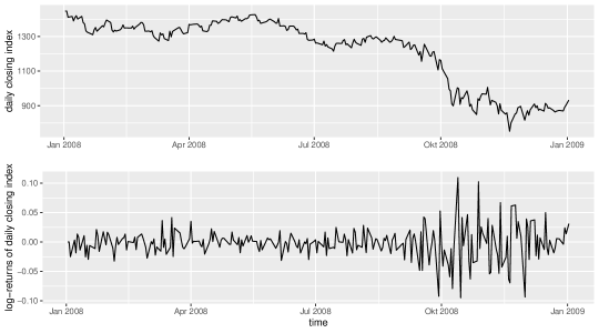
The analysis of financial time series, such as stock market prices, usually focuses on log returns instead of the observed data itself. As an example, we consider the log returns of the daily closing indices of Standard & Poor’s 500 (S&P 500, in short) defined by
where denotes the value of the index on day , in the period from January 2008 to December 2008; see Figure 1.
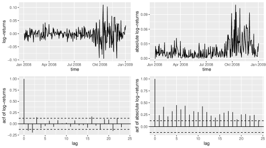
Comparing the plots of the sample autocorrelation function of the log returns and the sample autocorrelation function of their absolute values in Figure 2, we observe a phenomenon that is often encountered in the context of financial data: the log returns of the index appear to be uncorrelated, whereas the absolute log returns tend to be highly correlated.
Moreover, the plot in Figure 1 shows that the considered time series exhibits volatility clustering, meaning that large price changes, i.e., log returns with relatively large absolute values, tend to cluster. This indicates that observations are not independent across time, although the absence of linear autocorrelation suggests that the dependence is nonlinear; see Cont, (2005).
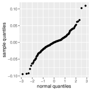
Another characteristic of financial time series is the occurrence of heavy tails. In particular, probability distributions of log returns often exhibit tails which are heavier than those of a normal distribution. For the S&P 500 data, this property is highlighted by the Q-Q plot in Figure 3.
All of the previously described features of financial data can be covered by the LMSV model considered in our paper.
In view of the fact that the LMSV model captures properties of the log returns of Standard & Poor’s 500 daily closing index, we are interested in analyzing the data with respect to a change in the tail index.
As in our simulations, we base the test decision on the statistic defined in (16). We choose , i.e., defines the proportion of the data that the estimation of the tail index is based on. Choosing , the value of the test statistic corresponds to . The 95%-quantile of the limit distribution equals . Choosing the critical value for the hypothesis test correspondingly, the value of therefore indicates a change-point in the tail index at a level of significance of 5%.
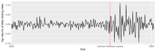
A natural estimate for the change-point location is given by that point in time , where attains its maximum. For the considered data, this point in time corresponds to September 16, 2008, i.e., one day after September 15, 2008, the day Lehman Brothers filed for bankruptcy protection; see Figure 4.
5 Proofs
5.1 Proof of Theorem 2.6
5.1.1 Decomposition of the tail empirical process
Recall that
where
To prove Theorem 2.6, we consider the following decomposition:
| where | ||||
Obviously, it holds that
for and . In particular, the convergence holds uniformly on compact subsets of . Moreover, for any it holds that
Note that
Due to Proposition 2.8 in Kulik and Soulier, (2011) and (TA.2) we have
which implies
Since
by (TA.3) and Breiman’s Lemma, it therefore suffices to study weak convergence of the process
For this, we consider the following decomposition:
| (17) |
where
and
| (18) |
We call the martingale part, while we refer to as the long-range dependent part.
5.1.2 The long-range dependent part
Proposition 5.1 (Weak convergence of ).
Proof.
Note that
| (19) |
and
As a result, we can rewrite as follows:
where
| (20) |
Due to regular variation of , we have
| (21) |
Furthermore, it holds that
| (22) |
where .
In the following, we will see that the first and the second summand in (22) are negligible. For this, it suffices to show that
Note that
Due to second order regular variation of , Lemma 6.1 implies that for any
Thus, it follows that
By (TA.2) and (TA.3), i.e., since and , it holds that
This completes the proof of Proposition 5.1. ∎
5.1.3 The martingale part
The goal of this section is to prove the following proposition:
Proposition 5.2.
Under the assumptions of Theorem 2.6, for any , the sequence , , converges in distribution to in , where denotes a standard Brownian sheet.
First, we establish convergence of the finite dimensional distributions. Then, we proceed with a proof of tightness. For the latter, we use chaining arguments; see Section 5.1).
The martingale part: Convergence of the finite dimensional distributions
We have to prove that for all positive integers and , all with and all , the vector with entries , , , converges in distribution to , , . For this, it suffices to consider the case . Indeed, if , we include , , in a decreasing order between and , i.e., such that , and if , we include , between and in an increasing order, i.e., . Letting , the convergence in distribution of the vector with entries , , , to , , , implies convergence of , , , to , , .
Let be an integer and let and be real numbers such that and . Define t intervals , and for , let . Moreover, define random variables
for .
Lemma 5.3.
The sequence of random vectors , , converges in distribution to , where the random variables , , are independent, and for all , the random variable is Gaussian, centered, and has variance , where .
This lemma directly provides convergence of the finite dimensional distributions, after having applied the continuous mapping theorem to the function
Proof of Lemma 5.3.
By the Cramér-Wold device, we have to prove that for each collection of real numbers , , the sequence , , converges to a normal distribution with mean zero and variance
| (23) |
We will prove this by applying the following central limit theorem for martingale difference arrays. For this, recall that , , , is a martingale difference array with respect to the filtration , , , if for all , , , is -measurable and .
Theorem 5.4 (Theorem VIII. 1 in Pollard, (1984)).
Let be a martingale difference array with respect to the filtration , such that is square integrable for all and . Moreover, assume that
-
1.
for each positive ,
(24) -
2.
(25)
Then, the sequence , , converges in distribution to a normal law with mean zero and variance defined in (23).
We express as a sum of martingale differences. For , define
If for some the integer satisfies , then we define
and if , we define .
In this way, and defining as the -algebra given by (18), the array , , , is a square integrable martingale difference array with respect to the filtration , , . Let us check (24). Observe that for all and , . Hence, for all ,
Consequently, for a fixed , when is such that , the indicator vanishes and hence (24) holds.
Let us check (25). It suffices to prove that for all
| (26) |
To this aim, we decompose :
Observe that using (19)
where we set for all . Moreover, it holds that
Hence, the expression on the left hand side of (26) is bounded by
where
Here we omit the dependence on in and in order to ease notations. We start with . Using stationarity, it suffices to prove that for all , , where
Applying Lemma 6.2 with , , and , we get
Using the ergodic theorem for the first term, the fact that allows us to conclude that as goes to infinity.
The treatment of and is the same: we take expectations and bound one of the factors using (43) in Lemma 6.2 when and (45) in Lemma 6.2 when . We then conclude by the dominated convergence theorem.
This finishes the proof of Lemma 5.3. ∎
The martingale part: Tightness
Lemma 5.5.
Proof.
Define
In order to prove tightness of , we validate the following tightness criterion: for all
Writing
it suffices to show
| (27) |
and
| (28) |
5.1.4 Proof of (27).
In order to prove (27), we apply a chaining technique.
For this, we define the intervals
for . Then, the expression inside in (27) is bounded by
| (29) |
In the following, we consider the first summand only, since for the second summand analogous considerations hold, i.e., it remains to show that
For this, it suffices to show that
We write , i.e., and . Note that
Define refining partitions for with , for , by
and choose such that
From the definition of we obtain
Then, with and , it follows that
As a result, we have
| (30) |
Since
it follows that
Additionally, we conclude that
For further estimation, we use Freedman’s inequality: if , , is a martingale difference sequence such that , where is a positive constant, then for all
see Theorem 1.6 in Freedman, (1975).
For this purpose, we define
Then, it follows that
Furthermore, for , which is chosen later, define
and
Since is continuous and since we can assume without loss of generality that is ultimately strictly decreasing, it holds that
and, consequently,
For an estimation by Freedman’s inequality, we have to specify . Choosing for some constant , where , , is a sequence with and , it follows (with ) that
for a corresponding choice of . Therefore, we have
As a result, an application of Freedman’s inequality yields
Noting that there exists a constant such that for all
elementary calculations yield
It follows that
Therefore, in order to finish the proof of (27), it remains to show that
Since for an event and a -algebra
it holds that
Therefore, we arrive at
Note that
| (31) |
where
so that
| (32) |
According to Lemma 6.2 in the appendix it holds that
Therefore, given Assumption (TA.2), it follows that
For the first summand in (31), it follows by Lemma 6.2 in the appendix that
According to Assumptions (TA.3) and (TA.4) the expectation of the summands on the right-hand side is finite and hence, for each ,
Finally, we consider the last summand in (31):
Obviously, depends neither on nor on . Due to the non-central limit theorem in Taqqu, (1979), it holds that
Choosing , it follows that
Hence, we have
5.1.5 Proof of (28).
Initially, note that
As before, we apply a chaining technique in order to prove (28). For this, we define the intervals
for .
5.2 Proof of Corollaries 2.7, 2.8, 2.10, and 2.11
Proof of Corollary 2.7.
An argument from Kulik and Soulier, (2011) is repeated and hence many technicalities are omitted. Note that the arguments below are model-free and only use the conclusion of Theorem 2.6.
It holds that
where
By substracting and adding , the following equality holds:
where if and if .
We note that, compared to Kulik and Soulier, (2011), the last term appears additionally due to the fact that we consider the two-parameter processes.
Rewriting as an integral and replacing by , we have
| (33) |
We will show weak convergence of the sequence
| (34) |
in by an application of the continuous mapping theorem. For this, we have to initially show that terms of the form are negligible. Noting that , it follows by Theorem 2.6 that
| (35) |
Indeed, Theorem 2.6 implies that in probability and
As a consequence, rewriting as
| (36) |
and combining Theorem 2.6 with (35) shows that the limit of the sequence corresponds to the limit of
| (37) |
By Theorem 2.6 and the continuous mapping theorem, we conclude that , , converges in distribution to , where it the limiting process in (11) or (12), respectively. Using the same arguments as in Kulik and Soulier, (2011), it can be shown that the convergence of , , can be easily extended to convergence of
| (38) |
Hence, we conclude that
in .
If , separation of the variables and shows that the limit vanishes. This finishes the proof of Corollary 2.7. ∎
Proof of Corollary 2.8.
Define
Then, it holds that
According to Skorokhod’s representation theorem (Theorem 2.3.4 in Shorack and Wellner, (1986)) and Theorem 2.6, we may assume without loss of generality that
where if , if , and denotes the corresponding limiting process in Theorem 2.6. In order to apply Vervaat’s Lemma as stated by Lemma 5 in Einmahl et al., (2010), we rephrase the above convergence as:
| (39) |
for any and with
Choosing , it follows that
As a result, Vervaat’s Lemma yields
| (40) |
Setting , we arrive at
The first two summands on the right-hand side converge to almost surely according to (39) and (40). Moreover, we have a.s. uniformly in and such that it follows by a continuity argument that the third summand converges to almost surely, as well.
6 Appendix: Second-order regular variation
The following lemmata originate in Kulik and Soulier, (2011) and are essential to the proof of Theorem 2.6.
Lemma 6.1 (Lemma 4.1 in Kulik and Soulier, (2011)).
Assume that . For positive there exists a constant such that
| (41) |
This implies that
| (42) |
Using boundedness of , we get the following simplified version of inequality (41):
| (43) |
We also need the following bound on the increments of .
Lemma 6.2 (Lemma 4.2 in Kulik and Soulier, (2011)).
Assume that . For positive there exists a constant such that for all and
| (44) |
Using again boundedness of , we get the following simplified version of inequality (44):
| (45) |
References
- Betken and Kulik, (2019) Betken, A. and Kulik, R. (2019). Testing for change in long-memory stochastic volatility time series. Journal of Time Series Analysis, 40(5):707 – 738.
- Bilayi-Biakana et al., (2019) Bilayi-Biakana, C., Ivanoff, G., and Kulik, R. (2019). The tail empirical process for long memory stochastic volatility models with leverage. Electronic Journal of Statistics, 13(2):3453 – 3484.
- Breidt et al., (1998) Breidt, F. J., Crato, N., and de Lima, P. (1998). The detection and estimation of long memory in stochastic volatility. Journal of Econometrics, 83(1 – 2):325 – 348.
- Breiman, (1965) Breiman, L. (1965). On some limit theorems similar to the arc-sin law. Teoriya Veroyatnostei i ee Primeneniya, 10:351 – 360.
- Cont, (2005) Cont, R. (2005). Long range dependence in financial markets. In Fractals in engineering, pages 159 – 179. Springer.
- Deo et al., (2006) Deo, R., Hsieh, M., Hurvich, C. M., and Soulier, P. (2006). Long memory in nonlinear processes. In Dependence in probability and statistics, volume 187 of Lecture Notes in Statistics, pages 221 – 244. Springer, New York.
- (7) Drees, H. (1998a). A general class of estimators of the extreme value index. Journal of Statistical Planning and Inference, 66(1):95 – 112.
- (8) Drees, H. (1998b). On smooth statistical tail functionals. Scandinavian Journal of Statistics, 25:187 – 210.
- Drees, (2000) Drees, H. (2000). Weighted approximations of tail processes for -mixing random variables. Annals of Applied Probability, 10(4):1274 – 1301.
- DuMouchel, (1983) DuMouchel, W. H. (1983). Estimating the stable index in order to measure tail thickness: a critique. Annals of Statistics, 11(4):1019 – 1031.
- Einmahl, (1990) Einmahl, J. H. J. (1990). The empirical distribution function as a tail estimator. Statistica Neerlandica, 44(2):79 – 82.
- Einmahl, (1992) Einmahl, J. H. J. (1992). Limit theorems for tail processes with application to intermediate quantile estimation. Journal of Statistical Planning and Inference, 32(1):137 – 145.
- Einmahl et al., (2010) Einmahl, J. H. J., Gantner, M., and Sawitzki, G. (2010). Asymptotics of the shorth plot. Journal of Statistical Planning and Inference, 140(11):3003 – 3012.
- Freedman, (1975) Freedman, D. A. (1975). On tail probabilities for martingales. The Annals of Probability, pages 100 – 118.
- Galbraith and Zernov, (2004) Galbraith, J. W. and Zernov, S. (2004). Circuit breakers and the tail index of equity returns. Journal of Financial Econometrics, 2(1):109 – 129.
- Hall, (1982) Hall, P. (1982). On some simple estimates of an exponent of regular variation. Journal of the Royal Statistical Society: Series B (Statistical Methodology), 44(1):37 – 42.
- Harvey, (2002) Harvey, A. C. (2002). Long memory in stochastic volatility. In Forecasting Volatility in the Financial Markets, pages 307 – 320. Butterwoth-Heinemann Finance.
- Hill, (1975) Hill, B. M. (1975). A simple general approach to inference about the tail of a distribution. Annals of Statistics, 3(5):1163 – 1174.
- Hoga, (2017) Hoga, Y. (2017). Change point tests for the tail index of -mixing random variables. Econometric Theory, 33(4):915 – 954.
- Hurvich and Soulier, (2009) Hurvich, C. M. and Soulier, P. (2009). Stochastic Volatility Models with Long Memory, pages 345 – 354. Springer.
- Kim and Lee, (2011) Kim, M. and Lee, S. (2011). Change point test for tail index for dependent data. Metrika, 74(3):297 – 311.
- Kim and Lee, (2012) Kim, M. and Lee, S. (2012). Change point test of tail index for autoregressive processes. Journal of the Korean Statistical Society, 41(3):305 – 312.
- Koedijk et al., (1990) Koedijk, K. G., Schafgans, M. M., and De Vries, C. G. (1990). The tail index of exchange rate returns. Journal of International Economics, 29(1-2):93 – 108.
- Kulik and Soulier, (2011) Kulik, R. and Soulier, P. (2011). The tail empirical process for long memory stochastic volatility sequences. Stochastic Processes and their Applications, 121(1):109 – 134.
- Mandelbrot, (1963) Mandelbrot, B. B. (1963). The Variation of Certain Speculative Prices. Business, 36:394 – 419.
- Mason, (1988) Mason, D. M. (1988). A strong invariance theorem for the tail empirical process. In Annales de l’IHP Probabilités et statistiques, volume 24, pages 491 – 506.
- Phillips et al., (1990) Phillips, P. C., Loretan, M., et al. (1990). Testing covariance stationarity under moment condition failure with an application to common stock returns. Technical report, Cowles Foundation for Research in Economics, Yale University.
- Pipiras and Taqqu, (2017) Pipiras, V. and Taqqu, M. S. (2017). Long-Range Dependence and Self-Similarity, volume 45. Cambridge University Press.
- Pollard, (1984) Pollard, D. (1984). Convergence of stochastic processes. Springer Series in Statistics. Springer-Verlag, New York.
- Quintos et al., (2001) Quintos, C., Fan, Z., and Phillips, P. (2001). Structural change tests in tail behaviour and the Asian crisis. The Review of Economic Studies, 68(3):633 – 663.
- Resnick and Stărică, (1997) Resnick, S. I. and Stărică, C. (1997). Asymptotic behavior of hill’s estimator for autoregressive data. Communications in Statistics. Stochastic Models, 13(4):703 – 721. Heavy tails and highly volatile phenomena.
- Rootzén, (2009) Rootzén, H. (2009). Weak convergence of the tail empirical process for dependent sequences. Stochastic Processes and their Applications, 119(2):468 – 490.
- Shorack and Wellner, (1986) Shorack, G. R. and Wellner, J. A. (1986). Empirical processes with applications to statistics. Wiley Series in Probability and Mathematical Statistics: Probability and Mathematical Statistics. John Wiley & Sons, Inc., New York.
- Taqqu, (1979) Taqqu, M. S. (1979). Zeitschrift für wahrscheinlichkeitstheorie und verwandte gebiete. Zeitschrift, 50(1):53 – 83.
- Taylor, (1986) Taylor, S. J. (1986). Modelling Financial Time Series. Wiley, New York.
- Werner and Upper, (2004) Werner, T. and Upper, C. (2004). Time variation in the tail behavior of Bund future returns. Journal of Futures Markets: Futures, Options, and Other Derivative Products, 24(4):387 – 398.