Risk-Aware Motion Planning for a Limbed Robot with Stochastic Gripping Forces Using Nonlinear Programming

Abstract

We present a motion planning algorithm with probabilistic guarantees for limbed robots with stochastic gripping forces. Planners based on deterministic models with a worst-case uncertainty can be conservative and inflexible to consider the stochastic behavior of the contact, especially when a gripper is installed. Our proposed planner enables the robot to simultaneously plan its pose and contact force trajectories while considering the risk associated with the gripping forces. Our planner is formulated as a nonlinear programming problem with chance constraints, which allows the robot to generate a variety of motions based on different risk bounds. To model the gripping forces as random variables, we employ Gaussian Process regression. We validate our proposed motion planning algorithm on an 11.5 kg six-limbed robot for two-wall climbing. Our results show that our proposed planner generates various trajectories (e.g., avoiding low friction terrain under the low risk bound, choosing an unstable but faster gait under the high risk bound) by changing the probability of risk based on various specifications.

I INTRODUCTION

Planning complex motions for limbed robots is challenging because planners need to design footsteps and a body trajectories while considering the robot kinematics and reaction forces. Motion planning for limbed robots has been studied by a number of researchers. Sampling-based planning, such as the Probabilistic-Roadmap (PRM), samples the environment and generates the motion while satisfying static equilibrium and kinematics for a robot [1], [2]. Optimization-based planning, such as Mixed-Integer Convex Programming (MICP) and Nonlinear Programming (NLP), solves the solution given constraints using optimization algorithms such as gradient descent [3]-[9].

While many papers discuss motion planning for the robot, few studies have investigated how planning is affected by stochastic gripping forces. One of the open problems in motion planning of a limbed robot equipped with grippers is the stochastic nature of gripping [10], [11]. For example, the gripping forces caused by spine grippers depend on the stochastically distributed asperity strength (Fig. 2). Thus, risk results from the randomness of the gripping force. By considering risk in a probabilistic manner, the planner can design a variety of trajectories based on various specifications.

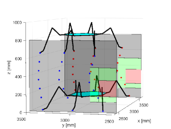
Figure 1: A planned trajectory for wall climbing that considers risk arising from slippery terrain. The black area shows a high friction area, the green area shows a low friction area, and the red area shows a zero friction area. Blue and red dots show the planned foot positions, and the hexagons show the body of the robot.

The stochastic planning problem can be categorized into two approaches: robust approaches [5]-[7], [12] and risk-bounded approaches [7], [8], [13]-[15]. In robust approaches, the planners design trajectories that guarantee the feasibility of the motion given the uncertainty bounds. A soft constraints-based robust planning was investigated in [6], where the planner allows the solution to be at the boundary of stability. Tas showed the planner to remain collision-free for the worst-case uncertainty for automated driving [12].

On the other hand, the risk-bounded approach designs trajectories that guarantee the feasibility of the motion given the probability density function (PDF): it prevents the probability of violating state constraints (violation probability) from being higher than a pre-specified probability. Prete formulated a chance-constrained optimization problem of a bipedal robot by approximating a joint chance constraints with linear inequality constraints [7]. Planning on slippery terrain was in [8], where the planner utilizes the prediction of the coefficient of friction to design the motion of the body and footsteps, respectively. Our approach is similar to [8], but we model the stochastic contact force of the robot and formulate the planning algorithm considering the trajectory of a body and footsteps simultaneously.

For tasks with a higher probability of failure (e.g., climbing on slippery terrain) [15], the risk-bounded approach has advantages over the robust approach. Because the robust approach often uses a much less informative deterministic model, it is likely to generate conservative solutions with the worst-case uncertainty bound. For demanding tasks, this may be infeasible, with such a planner generating no possible solution and failing to achieve specified goals. In contrast, because the risk-bounded approach can be more aggressive, the problem may be feasible, generating trajectories that carry a probability of failure through risk-taking alongside a non-zero chance of successfully achieving the goal. The violation probability provides a tuning knob to define a Pareto boundary on the risk between failure while finding a trajectory vs. failure while executing a found trajectory. This user-defined parameter can be task- and environment-specific, in contrast to the rigidity of the robust approach.

In this paper, we address a motion planning algorithm formulated as NLP for a limbed robot with stochastic gripping forces. Our proposed planner solves for stable postures and forces simultaneously with guaranteed bounded risk. In addition, chance constraints are introduced into the planner that restrict contact forces in a probabilistic manner. We employ a Gaussian Process (GP), a non-parametric Bayesian regression tool, to acquire the PDF of the gripping force. Our proposed motion planning algorithm is validated on an 11.5 kg hexapod robot with spine grippers for multi-surface climbing. While we focus on multi-surface robotic climbing with spine grippers in this paper, our proposed planner can be applied to other robots with any type of grippers for performing any task (e.g., planning of walking, grasping) as long as the robot has contact points with stochastic models.

The contributions of this paper are as follows:

1. We formulate risk-bounded NLP-based planning that considers the stochasticity of gripping forces.

2. We employ the Gaussian Process to model gripping forces as random variables.

3. We validate the algorithm in hardware experiments.

II PROBLEM FORMULATION

This section describes the friction cone considering maximum gripping forces, model of a position-controlled limbed robot with multi-contact surfaces, and the modeling process of a gripping force through GP.

II-A Friction Cone with Stochastic Gripping Forces

With grippers, the friction cone constraint can be relaxed on the contact point. For our spine-based gripper, even under a zero normal load, the spines insert into the microscopic gaps on the surface (Fig. 2), generating a significant amount of shear force (Fig. 6) [19]. For a magnet-based gripper, the reaction forces includes the additional magnetic force imposed by the gripper itself, offsetting the friction cone as seen by the rest of the robot.

Thus, we modify the regular friction cone, adding in an offset shear force when a normal force is zero to account for the gripping force. As the normal force increases, the maximal allowable shear force increase in the same way as a regular frictional force, with a coefficient of friction $\lambda$ that is assumed to be a constant only depending on the property of the contact surface. This contact model is illustrated in Fig. 3, where ${\mbox{\boldmath$f$}}^{r}$ is the reaction force between the surface and the gripper. ${\mbox{\boldmath$f$}}^{g,m}$ is the maximum gripping force from grippers under a zero normal force. Note that ${\mbox{\boldmath$f$}}^{g,m}$ is measured per gripper as a unit. In general, ${\mbox{\boldmath$f$}}^{g,m}$ can have both normal and shear components. However, for our spine grippers, the normal component of ${\mbox{\boldmath$f$}}^{g,m}$ is relatively small, so we assume that the gripper generates only shear adhesion. The gripper does not slip when ${\mbox{\boldmath$f$}}^{r}$ is within this friction cone, as indicated by the shaded region in Fig. 3. Since the interaction between the micro-spines and the surface is highly random, ${\mbox{\boldmath$f$}}^{g,m}$ is naturally modeled as a Gaussian random variable. However, the orientation of the spine and the number of spines in contact with the surface also change as the orientation of the gripper changes, which leads to a shift of the mean and standard deviation of ${\mbox{\boldmath$f$}}^{g,m}$. We learn this model from data by GP. With GP, our proposed planner is able to deal with the stochastic nature of gripping taking into account the gripper orientation.

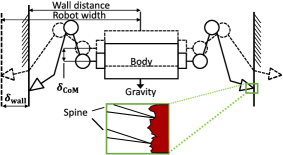
Figure 2: Deflection of a multi-limbed robot bracing between walls

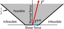
Figure 3: Friction cone considering stochastic gripping forces

II-B Model of Reaction Force Using Limb Compliance

During multi-surface locomotion, the robot leverages the compliance from its motors in order to squeeze itself between multi-surfaces, as depicted in Fig. 2. One difficulty multi-limbed robots have is that reaction forces are statically indeterminate [16]. Consequently, reaction forces cannot be determined by static equilibrium equations when the robot supports its weight more than three contact points. Hence, in order to calculate the reaction force under this condition, the deformation of the robotic system should be considered.

From the standard elasticity theory, ${\color[rgb]{0,0,0}{\mbox{\boldmath$f$}}^{r}}$ can be described as the spring force using the Virtual Joint Method [17]:

$${\color[rgb]{0,0,0}{\mbox{\boldmath$f$}}^{r}}={\mbox{\boldmath$K$}}\left({{\mbox{\boldmath$\delta$}}}_{\operatorname{wall}}-{{\mbox{\boldmath$\delta$}}}_{\operatorname{CoM}}\right)$$ (1)

$${\mbox{\boldmath$K=\left(Jk^{-1}J{{}^{\top}}\right)^{-1}$}},\ {\mbox{\boldmath$k$}}=diag(k_{i}),i=1,\ldots,{\color[rgb]{0,0,0}H}$$ (2)

where $K$ is the stiffness matrix for ${\color[rgb]{0,0,0}H}$ degree-of-freedom limb. $k$ is a diagonal matrix that has $k_{i}$ diagonal elements, and $k_{i}$ is the spring coefficients of the position-controlled servos. $J$ is a $3\times{\color[rgb]{0,0,0}H}$ Jacobian matrix. The deflection is imposed by terrain where ${{\mbox{\boldmath$\delta$}}}_{\operatorname{wall}}$ is the displacement of the terrain and ${\mbox{\boldmath$\delta$}}_{\operatorname{CoM}}$ is the body deflection, sag-down, due to the compliance as shown in Fig. 2.

II-C Model of Gripping Force Using Gaussian Process

The objective of using GP is to predict the maximum gripping force ${\mbox{\boldmath$f$}}^{g,m}$ in a probabilistic way.

There are many design decisions that go into the formulation of the GP problem, including choice of kernel, distance metric, and associated weighting between state variables [18]. We can start with the simplest formulation with all state variables equally weighted under the Euclidean distance metric using the squared exponential kernel as a starting point. In practice, this choice was observed to work well enough to not necessitate further design. A more general characterization of the effects of these hyperparameters can be found in [18]. In this work, we assume that the maximum gripping forces by spine grippers is a function of the gripper orientation and the coefficient of friction [10], [11], [19], [20]. This is because with a microscopic view, the spine-asperity interaction is different depending on how a spine is inclined with respect to the asperity as shown in Fig. 2. GP can handle the effects of other unmodeled parameters by treating them into uncertainty. Hence, the state $s$ is a four-dimensional vector with ${\mbox{\boldmath$s$}}=[\alpha,\beta,\gamma,\lambda]^{\top}$ where $\alpha$, $\beta$, $\gamma$ are the Euler angles along $x$, $y$, $z$ axis defined in Fig. 4.

Here, we assume that the maximum shear force follows Gaussian distribution. Given a data set $S=\left\{{\mbox{\boldmath$s$}}_{1},\cdots,{\mbox{\boldmath$s$}}_{n}\right\}$ with the measured shear forces ${\mbox{\boldmath$y$}}^{g,m}=\left[y^{g,m}_{1},\ldots,y^{g,m}_{n}\right]^{\top}$, the maximum shear force ${\mbox{\boldmath$f$}}^{g,m}$ by a gripper can therefore be modeled as:

$${\color[rgb]{0,0,0}{\mbox{\boldmath$f$}}^{g,m}({\mbox{\boldmath$s$}})}\sim\mathcal{GP}({\mbox{\boldmath$\mu$}}^{g,m}({\mbox{\boldmath$s$}}),{\mbox{\boldmath$\kappa$}}^{g,m}({\mbox{\boldmath$s$}},{\mbox{\boldmath$s_{*}$}}))$$ (3)

where, ${\mbox{\boldmath$f$}}^{g,m}=\left[f^{g,m}_{1},\ldots,f^{g,m}_{n}\right]^{\top}$, $n$ is the number of samples from a GP. ${\mbox{\boldmath$\mu$}}^{g,m}({\mbox{\boldmath$s$}})=\left[\mu^{g,m}_{1}({\mbox{\boldmath$s$}}),\ldots,\mu^{g,m}_{n}({\mbox{\boldmath$s$}})\right]^{\top}$ is the mean and ${\mbox{\boldmath$[$}}{\color[rgb]{0,0,0}{\mbox{\boldmath$\kappa$}}^{g,m}]_{i,j}}={\color[rgb]{0,0,0}\kappa^{g,m}}\left({\mbox{\boldmath$s$}}_{i},{\mbox{\boldmath$s$}}_{j}\right)$ is the covariance matrix, where $\kappa^{g,m}(\cdot,\cdot)$ is a positive definite kernel. In this work, we employ the squared exponential kernel as follows:

$${\color[rgb]{0,0,0}\kappa^{g,m}}\left({\mbox{\boldmath$s$}}_{i},{\mbox{\boldmath$s$}}_{j}\right)=\sigma_{f}^{2}\exp\left(-\frac{1}{2}\frac{\left|{\mbox{\boldmath$s$}}_{i}-{\mbox{\boldmath$s$}}_{j}\right|^{2}}{\ell^{2}}\right)$$ (4)

where $\sigma_{f}^{2}$ represents the amplitude parameter and $l$ defines the smoothness of the function ${\mbox{\boldmath$f$}}^{g,m}$.

Here, let ${\mbox{\boldmath$D$}}=[{\mbox{\boldmath$s$}}_{1},\cdots,{\mbox{\boldmath$s$}}_{n}]^{\top}$ be the matrix of the inputs. In order to predict the mean and variance matrix at ${\mbox{\boldmath$D$}}_{*}$, we obtain the predictive mean and variance of the maximum shear force by assuming that it is jointly Gaussian as follows:

$${\color[rgb]{0,0,0}\hat{{\mbox{\boldmath$f$}}}^{g,m}}=\mathbb{E}\left[{\mbox{\boldmath$f$}}^{g,m}\left({\mbox{\boldmath$D$}}_{*}\right)\right]={\mbox{\boldmath$\kappa$}}_{*}^{\top}\left({\mbox{\boldmath$K$}}_{D}+\sigma_{n}^{2}{\mbox{\boldmath$I$}}\right)^{-1}{\mbox{\boldmath$y$}}_{g}$$ (5)

$${\color[rgb]{0,0,0}\hat{{\mbox{\boldmath$\Sigma$}}}^{g,m}}=\mathbb{V}\left[{\mbox{\boldmath$f$}}^{g,m}\left({\mbox{\boldmath$D$}}_{*}\right)\right]={\mbox{\boldmath$\kappa$}}_{**}-{\mbox{\boldmath$\kappa$}}_{*}^{\top}\left({\mbox{\boldmath$K$}}_{D}+\sigma_{n}^{2}{\mbox{\boldmath$I$}}\right)^{-1}{\mbox{\boldmath$\kappa$}}_{*}$$ (6)

where ${\mbox{\boldmath$\kappa$}}_{*}={\mbox{\boldmath$\kappa$}}^{g,m}\left(D_{*},D\right)$, ${\mbox{\boldmath$K$}}_{D}={\mbox{\boldmath$\kappa$}}^{g,m}\left(D,D\right)$, ${\mbox{\boldmath$\kappa$}}_{**}={\mbox{\boldmath$\kappa$}}^{g,m}\left(D_{*},D_{*}\right)$, and $\sigma_{n}^{2}$ is the variance of the Gaussian observation noise with zero mean.

Our GP procedure can be generalizable to model other gripping forces as long as the gripping force changes continuously as the orientation of the gripper changes. For instance, the GP approach can be used to model the gecko gripper force [21] using the detachment angle as the state of the GP.

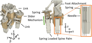
Figure 4: Mechanical design of the spine gripper

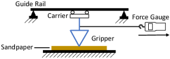
Figure 5: Experiment setup to evaluate maximum gripping forces on sandpaper

II-D Spine Gripper for Wall Climbing

A three-finger spine-based gripper was designed (Fig. 4) using spine cells based on [20]. Each finger consists of a spine cell with 25 machine needles loaded with 5 mN/mm springs, and a slider mechanism holds the cell with one compliant plastic spring. The diameter of the needle at the tip is 0.93 mm, and it is made of carbon steel. The gripper center module includes one spine palm with the same spine configurations as the cells. The attachment component is fixed at the tip of the robot limb at $37\mathrm{°}$ from the limb axis to maximize the contact area. The finger, center, and attachment members are assembled with a one-slider, two linkage mechanism (Fig. 4). This linkage system is designed to provide a passive micro grip as the center palm presses up against a wall. The three fingers are located at $120\mathrm{°}$ apart from each other in $z$-axis and tilted about $15\mathrm{°}$ from $z$-axis.

II-E Data Collection

TABLE I: Varied orientations for collecting datasets of GP

Training	$\alpha,\beta=$$,$$,$$$, $\gamma=$$,$$,$$$, $\lambda=1.1,2.3$
Testing	$\alpha=$$,$$,\cdots,$$|\{\beta=$$,\gamma=$$,\lambda=2.3$}
	$\beta=$$,$$,\cdots,$$|\{\alpha=$$,\gamma=$$,\lambda=2.3$}
	$\gamma=$$,$$,$$,\cdots,$$|\{\alpha=$$,\beta=$$,\lambda=2.3$}
	$\lambda=1.1,1.4,1.82,2.3|\{\alpha=$$,\beta=$$,\gamma=$$$}

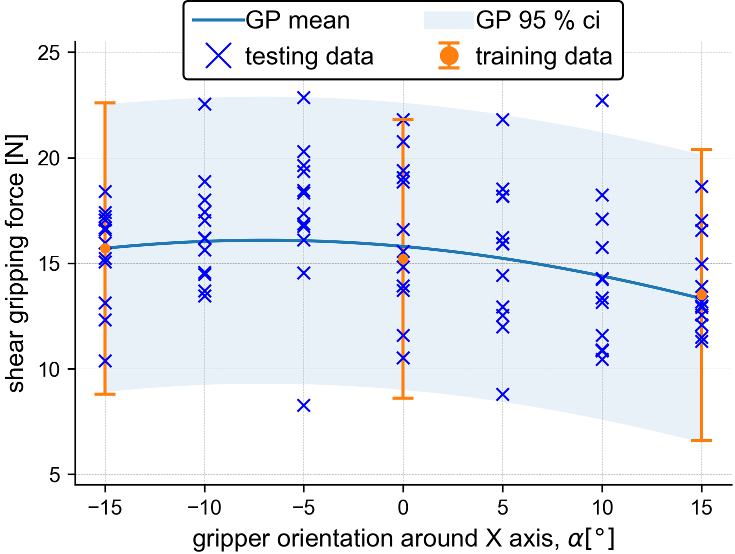
(a) $\beta=$$,\gamma=$$,\lambda=2.3$

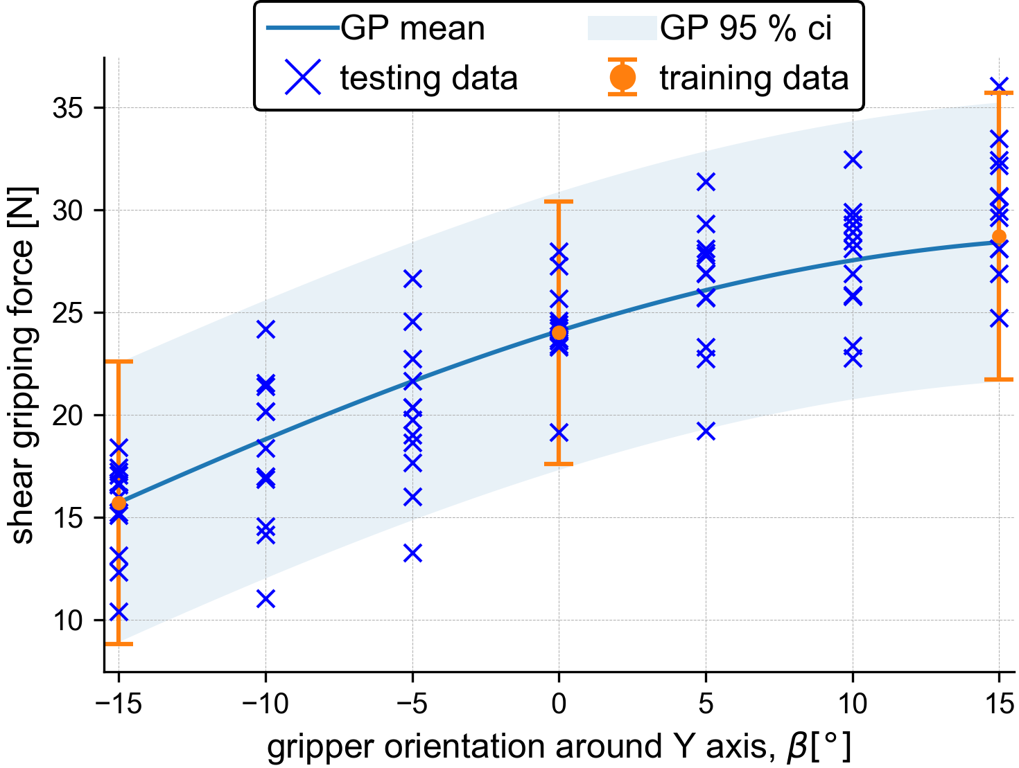
(b) $\alpha=$$,\gamma=$$,\lambda=2.3$

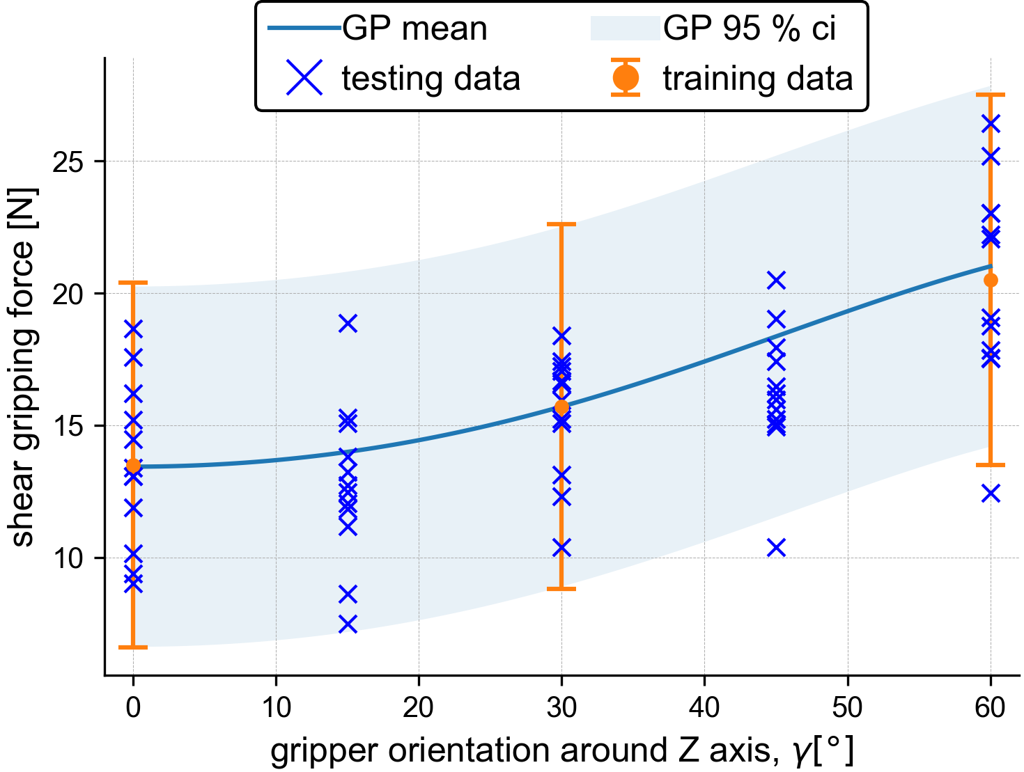
(c) $\alpha=$$,\beta=$$,\lambda=2.3$

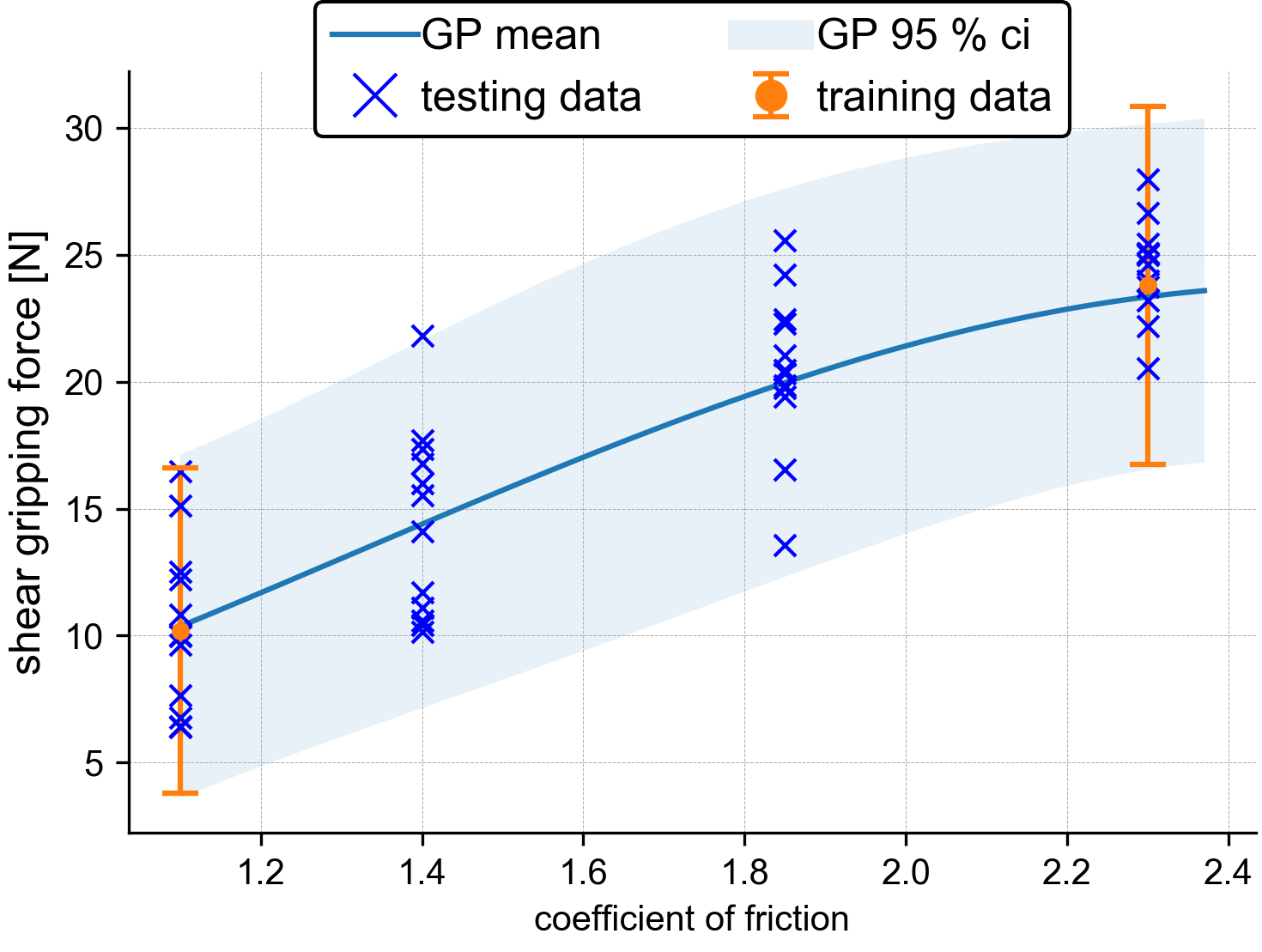
(d) $\alpha=$$,\beta=$$,\gamma=0$

Figure 6: The predicted maximum gripping force PDF from GP, the training data PDF, and the testing dataset

To collect a dataset, maximum gripping forces ${\mbox{\boldmath$f$}}^{g,m}$ were evaluated with a minimal normal force at varied orientations as summarized in Table I. We collected 20 data sequences for every orientation as a training dataset and 10 data sequences as a testing dataset. The coefficient of friction between spines and environments was measured by loading a constant mass on the gripper. A small activation force is necessary to compress spine springs and ensure that the spines are touching the wall, but is assumed to be negligible. These orientations were selected to cover possible gripper angles during regular wall climbing. The gripper was fixed to a linear slider at an orientation and pulled by a force gauge on 36-grit and 80-grit sandpapers that are commonly used to emulate rough surface with microscopic asperities [20], as shown in Fig. 5. The GP hyperparameters were optimized using the BFGS algorithm [22]. The obtained testing data with the predicted PDF of the maximum gripping force and the PDF of the training data is illustrated in Fig. 6. The predicted maximum gripping force and the training data are displayed as a mean $\pm$ with a 95 % confidence interval. Overall, we show that the GP prediction works well with different states.

III RISK-AWARE MOTION PLANNING

In this section, we present a complete risk-aware motion planning algorithm formulated as (8a)-(8k). The objective of our proposed planner is to find the optimal trajectory for the Center of Mass (CoM) position, its orientation, the foot position, and the reaction force for each foot in order to arrive at the destination while satisfying constraints. Our proposed planner enables the robot to find feasible trajectories that consider risk from the grippers under various environments.

We define one round of movement made by a robot when its body and all of its limbs have moved onto the next footholds. Note that for each round, the planner investigates several critical instants between two postures with pre-defined gait as explained in detail in Section IV. At $j$-th round, $\Gamma$ is the decision variables that are given as:

$$\Gamma=\{{\mbox{\boldmath$p$}}_{i,j},{{\mbox{\boldmath$P$}}}_{\operatorname{CoM},j},{{\mbox{\boldmath$\Theta$}}}_{\operatorname{CoM},j},{{\mbox{\boldmath$\theta$}}}_{i,j},{\mbox{\boldmath$f$}}^{r}_{i,j},{\color[rgb]{0,0,0}\hat{{\mbox{\boldmath$f$}}}_{i,j}^{g,m},\hat{{\mbox{\boldmath$\Sigma$}}}_{i,j}^{g,m}}\}$$ (7)

where ${\mbox{\boldmath$p$}}_{i,j}$ is the foot $i$ position, ${{\mbox{\boldmath$P$}}}_{\operatorname{CoM},j}$ is the position of the body, ${{\mbox{\boldmath$\Theta$}}}_{\operatorname{CoM},j}$ is the orientation of the body, ${{\mbox{\boldmath$\theta$}}}_{i,j}$ are the joint angles for the limb $i$, and

$$\underset{\Gamma}{\operatorname{minimize}}\ \color[rgb]{0,0,0}\Psi_{tot}$$ (8a)

s.t., for each round $$j=1,\ldots,N$$

and for each limb $$i=1,\ldots,L$$

$$|\Delta{\mbox{\boldmath$P$}}_{\operatorname{CoM}}|\leq\Delta{\mbox{\boldmath$P$}}_{\operatorname{Th}} \color[rgb]{0,0,0}\operatorname{(linear\ stride)}$$ (8b)

$$|\Delta{\mbox{\boldmath$\Theta$}}_{\operatorname{CoM}}|\leq\Delta{\mbox{\boldmath$\Theta$}}_{\operatorname{Th}} \color[rgb]{0,0,0}\operatorname{(angular\ stride)}$$ (8c)

$$|\Delta{\mbox{\boldmath$p$}}_{i}|\leq\Delta{\mbox{\boldmath$p$}}_{\operatorname{Th}} \color[rgb]{0,0,0}\operatorname{(foot\ stride)}$$ (8d)

$$\mathbf{{\mbox{\boldmath$p$}}}_{i,j}\in\mathcal{R}({\mbox{\boldmath$P$}}_{\operatorname{CoM},j},{\mbox{\boldmath$\Theta$}}_{\operatorname{CoM},j},{\mbox{\boldmath$\theta$}}_{i,j}) \color[rgb]{0,0,0}\operatorname{(kinematics)}$$ (8e)

$$\color[rgb]{0,0,0}\mathbf{{\mbox{\boldmath$p$}}}_{i,j}\in\mathcal{T} \color[rgb]{0,0,0}\operatorname{(contact\ region)}$$ (8f)

$$\color[rgb]{0,0,0}\sum_{i=1}^{L}{\mbox{\boldmath$f$}}^{r}_{i,j}+{\mbox{\boldmath$F$}}_{tot}={\mbox{\boldmath$0$}} \color[rgb]{0,0,0}\operatorname{(force\ eqm)}$$ (8g)

$$\color[rgb]{0,0,0}\sum_{i=1}^{L}\left({\mbox{\boldmath$p$}}_{i,j}\times{\mbox{\boldmath$f$}}^{r}_{i,j}\right)+{\mbox{\boldmath$M$}}_{tot}={\mbox{\boldmath$0$}} \color[rgb]{0,0,0}\operatorname{(moment\ eqm)}$$ (8h)

$${\mbox{\boldmath$\tau$}}_{i,j}={\mbox{\boldmath$J$}}\left({\mbox{\boldmath$\theta$}}_{i,j}\right)^{\top}\color[rgb]{0,0,0}{\mbox{\boldmath$f$}}^{r}_{i,j} \color[rgb]{0,0,0}\operatorname{(joint\ torque)}$$ (8i)

$$\left\|{\mbox{\boldmath$\tau$}}_{i,j}\right\|_{2}\leq{\mbox{\boldmath$\tau$}}_{\operatorname{Th}} \color[rgb]{0,0,0}\operatorname{(torque\ limit)}$$ (8j)

$${\mbox{\boldmath$f$}}^{r}_{i,j}\in\mathcal{F}\left({\color[rgb]{0,0,0}\lambda}_{i,j}({\mbox{\boldmath$p$}}_{i,j}),{\mbox{\boldmath$n$}}_{i,j},{\color[rgb]{0,0,0}{\mbox{\boldmath$f$}}^{g,m}_{i,j}}\right) {\color[rgb]{0,0,0}\operatorname{(friction\ cone)}}$$ (8k)

${\mbox{\boldmath$f$}}^{r}_{i,j}$ is defined in Section II-A. In this study, ${\mbox{\boldmath$f$}}^{g,m}_{i,j}$ is treated as a random variable based on the model of GP, which follows ${\mbox{\boldmath$f$}}^{g,m}_{i,j}\sim N\left(\hat{{\mbox{\boldmath$f$}}}_{i,j}^{g,m}(s_{i,j}),\hat{{\mbox{\boldmath$\Sigma$}}}_{i,j}^{g,m}(s_{i,j})\right)$. Equation (8a) is the cost function that depends on the robot’s state. Equation (8b), (8c), and (8d) bound the range of travel between rounds. Equation (8e) represents the forward kinematics constraints. In (8f), it ensures that ${\mbox{\boldmath$p$}}_{i,j}$ is within the feasible terrain where the robot is able to put its limb. In this paper, we assume that the robot generates a quasi-static motion. Hence, the planner has the static equilibrium constraints expressed by (8g) and (8h), where ${\mbox{\boldmath$F$}}_{tot}$ and ${\mbox{\boldmath$M$}}_{tot}$ is the external force and moment, respectively. In this work, only gravity is considered as the external force. Equation (8i) and (8j) ensure that the motor torque is lower than the maximum motor torque where $J\left({\mbox{\boldmath$\theta$}}_{i}\right)$ is a Jacobian matrix. The reaction force ${\mbox{\boldmath$f$}}^{r}_{i}$ is constrained by (8k), which describes the friction cone constraints to prevent the robot from slipping where ${\lambda}_{i,j}({\mbox{\boldmath$p$}}_{i,j})$ denotes the coefficient of friction at ${\mbox{\boldmath$p$}}_{i,j}$. Note that this constraints (8k) is also stochastic constraints due to ${\mbox{\boldmath$f$}}^{r}_{i}$. Equation (8k) can be converted into deterministic constraints, which is explained in Section III-B.

Compared to sampling-based approaches such as RRT, NLP is able to formulate relatively complicated constraints such as friction cone constraints (8k), which are typically difficult for the sampling-based approaches to handle in terms of computation. In addition, MICP approaches such as [3], [5], [9] can increase the computation speed by decoupling the pose state from wrench states. However, they potentially limit the robot’s mobility. The robot may not choose the trajectory on the low friction terrain in case the planner first solves the pose problem and then solves the wrench problem later since the pose optimization problem does not consider the wrench information. Although MICP can plan the trajectories considering both wrench and pose state simultaneously, it needs to sacrifice the accuracy by assuming an envelope approximation on bilinear terms [3] or allow relatively expensive computation as the number of the integer variables increases, which is intractable for high degree-of-freedom (DoF) robots (e.g., our robot has 24 DoF). In contrast, NLP can simultaneously solve the trajectory reasoning both the pose and the wrench with relatively less computation [4].

III-A Deterministic Constraints

Here, we explain two deterministic constraints (8e), (8f), that are not explicitly shown in (8a)-(8k).

III-A1 Kinematics

Forward kinematics (8e) is given as:

$${{\mbox{\boldmath$p$}}}_{i,j}={{\mbox{\boldmath$R$}}({\mbox{\boldmath$\Theta$}}_{\operatorname{CoM},j}){\mbox{\boldmath$p$}}^{b}_{i,j}+{\mbox{\boldmath$P$}}_{\operatorname{CoM},j}}$$ (9)

where ${\mbox{\boldmath$R$}}({\mbox{\boldmath$\Theta$}}_{\operatorname{CoM}})$ is the rotation matrix from the world frame to the body frame, ${\mbox{\boldmath$p$}}^{b}_{i}$ is the foot position relative to the body frame.

III-A2 Feasible Contact Regions

We utilize NLP to formulate the planning algorithm so that any nonlinear terrain (i.e., non-flat terrain), such as tube and curve, can be directly described.

If a robot traverses on the flat terrain, the footstep regions are convex polygons as follows:

$${\mbox{\boldmath$C$}}_{r}{\mbox{\boldmath$p$}}_{i,j}\leq{\mbox{\boldmath$D$}}_{r}$$ (10)

III-B Chance Constraints

Here, we show that the friction cone constraints in (8k) can be expressed using chance constraints, which allow the planner to convert the stochastic constraints into deterministic constraints.

One key characteristic of robotic climbing is that climbing is a highly risky operation: a robot can easily fall without planning its motion correctly. Hence, it needs to restrict reaction forces using the friction cone constraints given as:

$${\mbox{\boldmath$n$}}_{i,j}^{\top}{\mbox{\boldmath$f$}}_{i,j}^{r}\geq 0$$ (11)

$$\left\|{\mbox{\boldmath$f$}}_{i,j}^{r}-\left({\mbox{\boldmath$n$}}_{i,j}^{\top}{\mbox{\boldmath$f$}}_{i,j}^{r}\right){\mbox{\boldmath$n$}}_{i,j}^{\top}\right\|_{2}\leq{\color[rgb]{0,0,0}\lambda}_{i}\left({\mbox{\boldmath$n$}}_{i,j}^{\top}{\mbox{\boldmath$f$}}_{i,j}^{r}\right){\color[rgb]{0,0,0}+{\mbox{\boldmath$f$}}_{i,j}^{g,m}}$$ (12)

To decrease the computation of solving for the NLP solver, we simplify the (12) by linearizing them as follows:

$$\left|{\mbox{\boldmath$\zeta$}}_{i,j}^{\top}{\mbox{\boldmath$f$}}_{i,j}^{r}\right|\leq{\lambda}_{i}\left({\mbox{\boldmath$n$}}_{i}^{\top}{\mbox{\boldmath$f$}}_{i,j}^{r}\right){\color[rgb]{0,0,0}+{\mbox{\boldmath$f$}}_{i,j}^{g,m}}$$ (13)

$$\left|{\mbox{\boldmath$\xi$}}_{i,j}^{\top}{\mbox{\boldmath$f$}}_{i,j}^{r}\right|\leq{\lambda}_{i}\left({\mbox{\boldmath$n$}}_{i}^{\top}{\mbox{\boldmath$f$}}_{i,j}^{r}\right){\color[rgb]{0,0,0}+{\mbox{\boldmath$f$}}_{i,j}^{g,m}}$$ (14)

where ${\mbox{\boldmath$\zeta$}}_{i,j}$, ${\mbox{\boldmath$\xi$}}_{i,j}$ are any tangential direction vectors on the wall plane.

Regarding (8k) formulated as (11), (13), (14), we rearrange the equations and the joint chance constraint is given by:

$${\color[rgb]{0,0,0}\operatorname{Pr}\left(\bigwedge_{j=1,\ldots,N}\bigwedge_{k=1,\ldots,M}{\mbox{\boldmath$\alpha$}}_{i,j}^{k\top}{\mbox{\boldmath$f$}}_{i,j}^{g,m}\leq\beta_{i,j}^{k}\right)\geq 1-\Delta_{\operatorname{}}}$$ (15)

where ${\mbox{\boldmath$\alpha$}}_{i,j}^{k}$ are coefficient vectors, and $\beta_{i,j}^{k}$ are coefficient scalars that consist of the convex polytopes defined in (11), (13), (14). In (15), $M$ denotes the number of constraints defining the polytopes. $\Delta_{\operatorname{}}$ is the user-defined violation probability, where the probability of violating constraints is under the $\Delta_{\operatorname{}}$. We can regard $\Delta$ as relating to the likelihood that gripper slip will be responsible for the failure of the robot. For example, if $\Delta_{\operatorname{}}$ is high, the planner can explore a larger space because the feasible region expands in optimization. As a result, the robot tends to plan a trajectory with a high violation probability by assuming that the gripper generates enough force. For a robotic climbing task, these chance constraints enable the robot to perform challenging motions that would be infeasible without considering the gripping force. In contrast, if $\Delta_{\operatorname{}}$ is small, the planner tends to generate more conservative motions because the robot assumes that the gripper does not output enough force to support the weight of the robot.

Imposing (15) is computationally intractable. Thus, using Boole’s inequality, Blackmore [13], showed that the feasible solution to (15) is the feasible solution to the following equations:

$${\color[rgb]{0,0,0}\operatorname{Pr}\left({\mbox{\boldmath$\alpha$}}_{i,j}^{k\top}{\mbox{\boldmath$f$}}_{i,j}^{g,m}\leq\beta_{i,j}^{k}\right)\geq 1-\Delta_{j,k}}$$ (16)

$$\sum_{j=1}^{N}\sum_{k=1}^{M}\Delta_{j,k}\leq\Delta_{\operatorname{}}$$ (17)

for all $j=1,\ldots,N,\quad k=1,\ldots,M$. The violation probability for each constraint per round $\Delta_{j,k}$ is constrained in (17), in order not to exceed the given $\Delta_{\operatorname{}}$. Because non-uniform risk allocation (17) is also computationally expensive [14], we use the following relation:

$$\color[rgb]{0,0,0}{\Delta_{j,k}}=\frac{\Delta_{\operatorname{}}}{NM}$$ (18)

${\mbox{\boldmath$\alpha$}}_{i,j}^{k\top}{\mbox{\boldmath$f$}}_{i,j}^{g,m}$ is a multivariate Gaussian distribution such that ${\mbox{\boldmath$\alpha$}}_{i,j}^{k\top}{\mbox{\boldmath$f$}}_{i,j}^{g,m}\sim N\left({\mbox{\boldmath$\alpha$}}_{i,j}^{k\top}\hat{{\mbox{\boldmath$f$}}}_{i,j}^{g,m},{\mbox{\boldmath$\alpha$}}_{i,j,k\top}\hat{{\mbox{\boldmath$\Sigma$}}}^{g,m}_{i,j}{\mbox{\boldmath$\alpha$}}_{i,j}^{k}\right)$. Thus, the stochastic constraints (16) can be then converted into a deterministic constraint as given by:

$$\begin{split}\color[rgb]{0,0,0}\operatorname{Pr}\left({\mbox{\boldmath$\alpha$}}_{i,j}^{k\top}{\mbox{\boldmath$f$}}_{i,j}^{g,m}\leq\beta_{i,j}^{k}\right)&=\color[rgb]{0,0,0}\Phi\left(\frac{\beta_{i,j}^{k}-{\mbox{\boldmath$\alpha$}}_{i,j}^{k\top}\hat{{\mbox{\boldmath$f$}}}_{i,j}^{g,m}}{\sqrt{{\mbox{\boldmath$\alpha$}}_{i,j}^{k\top}\hat{{\mbox{\boldmath$\Sigma$}}}^{g,m}_{i,j}{\mbox{\boldmath$\alpha$}}_{i,j}^{k}}}\right)\\ &\color[rgb]{0,0,0}\geq 1-\Delta_{j,k}\end{split}$$ (19)

where $\Phi$ is the cumulative distribution function of the standard normal distribution. It can be transformed further as follows:

$$\color[rgb]{0,0,0}{\mbox{\boldmath$\alpha$}}_{i,j}^{k\top}\hat{{\mbox{\boldmath$f$}}}_{i,j}^{g,m}+\sqrt{{\mbox{\boldmath$\alpha$}}_{i,j}^{k\top}\hat{{\mbox{\boldmath$\Sigma$}}}^{g,m}_{i,j}{\mbox{\boldmath$\alpha$}}_{i,j}^{k}}\Phi^{-1}\left(1-\Delta_{j,k}\right)\leq\beta_{i,j}^{k}$$ (20)

where $\Phi^{-1}$ is the inverse function of $\Phi$.

III-C Cost Function

The cost function consists of intermediate costs and a terminal cost. In this work, the target mission is to arrive at the destination. Thus, the terminal cost is the distance from the position of the last pose to the destination.

$${\color[rgb]{0,0,0}\Psi_{\operatorname{D}}}=\left({{\mbox{\boldmath$q$}}}_{N}-{{\mbox{\boldmath$q$}}}_{D}\right)^{\top}{\mathbf{W}}_{\operatorname{D}}\left({{\mbox{\boldmath$q$}}}_{N}-{{\mbox{\boldmath$q$}}}_{d}\right)$$ (21)

where ${\mathbf{W}}_{\operatorname{D}}$ is the weighting matrix and ${{\mbox{\boldmath$q$}}}_{N}=\left[{{\mbox{\boldmath$p$}}}_{1,N},\ldots,{{\mbox{\boldmath$p$}}}_{L,N}\right]$ while ${{\mbox{\boldmath$q$}}}_{d}$ is the configuration at the destination. The intermediate costs restrict a large amount of shifting in terms of linear and rotational motion of a body and the foot position as follows:

$${\color[rgb]{0,0,0}\Psi_{\operatorname{BPos}}}=\Delta{{\mbox{\boldmath$P$}}}_{\operatorname{CoM}}^{\top}{\mathbf{W}}_{\operatorname{BPos}}\Delta{{\mbox{\boldmath$P$}}}_{\operatorname{CoM}}$$ (22)

$${\color[rgb]{0,0,0}\Psi_{\operatorname{Foot}}}=\sum_{i=1}^{L}\Delta{{\mbox{\boldmath$p$}}}_{i}^{\top}{\mathbf{W}}_{\operatorname{Foot}}\Delta{{\mbox{\boldmath$p$}}}_{i}$$

$${\color[rgb]{0,0,0}\Psi_{\operatorname{BRot}}}=\Delta{\Theta}_{\operatorname{CoM}}^{\top}\mathbf{{W}_{\operatorname{BRot}}}\Delta{\Theta}_{\operatorname{CoM}}$$

where ${\mathbf{W}}_{\operatorname{BPos}}$, ${\mathbf{W}}_{\operatorname{Foot}}$, and ${\mathbf{W}}_{\operatorname{BRot}}$ are the weighting matrix.

III-D Two Step Optimization for a Position-Controlled Robot

Although our proposed motion planner works for any limbed robot, there is a drawback for a position-controlled robot when wall-climbing. For the position-controlled robot, it is necessary to compute how much ${{\mbox{\boldmath$\delta$}}}_{\operatorname{wall}}$ is necessary to generate the planned reaction forces. Therefore, the planner needs to include additional constraints from (1), (2) to realize the planned trajectory. However, we observed that the nonlinear solver has a numerical issue with (2), so it is intractable for the solver to solve our proposed NLP in (8a)-(8k) with (1), (2). To avoid this problem, we decouple the optimization problem into two-step problems shown in (23a)-(23l) and (24a)-(24d):

$$\underset{\Gamma}{\operatorname{minimize}}\ \color[rgb]{0,0,0}\Psi_{\operatorname{D}}+\sum_{j=1}^{N-1}(\Psi_{\operatorname{BPos}}+\Psi_{\operatorname{Foot}}+\Psi_{\operatorname{BRot}})$$ (23a)

$$\text{s.t.}|{\mbox{\boldmath$P$}}_{\operatorname{CoM},j+1}-{\mbox{\boldmath$P$}}_{\operatorname{CoM},j}|\leq\Delta{\mbox{\boldmath$P$}}_{\operatorname{Th}}$$ (23b)

$$|{\mbox{\boldmath$\Theta$}}_{\operatorname{CoM},j+1}-{\mbox{\boldmath$\Theta$}}_{\operatorname{CoM},j}|\leq\Delta{\mbox{\boldmath$\Theta$}}_{\operatorname{Th}}$$ (23c)

$$|{\mbox{\boldmath$p$}}_{i,j+1}-{\mbox{\boldmath$p$}}_{i,j}|\leq\Delta{\mbox{\boldmath$p$}}_{\operatorname{Th}}$$ (23d)

$${{\mbox{\boldmath$p$}}}_{i,j}={{\mbox{\boldmath$R$}}({\mbox{\boldmath$\Theta$}}_{\operatorname{CoM},j}){\mbox{\boldmath$p$}}^{b}_{i,j}+{\mbox{\boldmath$P$}}_{\operatorname{CoM},j}}$$ (23e)

$${\mbox{\boldmath$C$}}_{r}{\mbox{\boldmath$p$}}_{i,j}\leq{\mbox{\boldmath$D$}}_{r}$$ (23f)

$$\color[rgb]{0,0,0}\sum_{i=1}^{L}{{\mbox{\boldmath$f$}}}_{i,j}^{r}+{\mbox{\boldmath$F$}}_{tot}={\mbox{\boldmath$0$}}$$ (23g)

$$\color[rgb]{0,0,0}\sum_{i=1}^{L}\left({\mbox{\boldmath$p$}}_{i,j}\times{{\mbox{\boldmath$f$}}}_{i,j}^{r}\right)+{\mbox{\boldmath$M$}}_{tot}={\mbox{\boldmath$0$}}$$ (23h)

$${\mbox{\boldmath$\tau$}}_{i,j}={\mbox{\boldmath$J$}}\left({\mbox{\boldmath$\theta$}}_{i,j}\right)^{\top}{\color[rgb]{0,0,0}{\mbox{\boldmath$f$}}^{r}_{i,j}}$$ (23i)

$$\left\|{\mbox{\boldmath$\tau$}}_{i,j}\right\|_{2}\leq\Delta{\mbox{\boldmath$\tau$}}$$ (23j)

$$\color[rgb]{0,0,0}{\mbox{\boldmath$\alpha$}}_{i,j}^{k\top}\hat{{\mbox{\boldmath$f$}}}_{i,j}^{g,m}+\sqrt{{\mbox{\boldmath$\alpha$}}_{i,j}^{k\top}\hat{{\mbox{\boldmath$\Sigma$}}}^{g,m}_{i,j}{\mbox{\boldmath$\alpha$}}_{i,j}^{k}}\Phi^{-1}\left(1-\Delta_{j,k}\right)\leq\beta_{i,j}^{k}$$ (23k)

$${\color[rgb]{0,0,0}{\Delta_{j,k}}=\frac{\Delta_{\operatorname{}}}{NM}}$$ (23l)

$${\operatorname{find}}\ {\mbox{\boldmath$\delta$}}_{\operatorname{wall},i,j},{\mbox{\boldmath$\delta$}}_{\operatorname{CoM},i,j}$$ (24a)

$$\text{s.t.}\left\|{\mbox{\boldmath$\delta$}}_{\operatorname{wall},i,j}\right\|_{2}\leq{\mbox{\boldmath$\delta$}}_{\operatorname{Th,wall},i,j}$$ (24b)

$${\color[rgb]{0,0,0}{\mbox{\boldmath$f$}}^{r}_{i,j}}={\mbox{\boldmath$K$}}_{i}\left({\mbox{\boldmath$\delta$}}_{\operatorname{wall},i,j}-{\mbox{\boldmath$\delta$}}_{\operatorname{CoM},i,j}\right)$$ (24c)

$$K_{i,j}=\left({\mbox{\boldmath$J$}}\left({\mbox{\boldmath$\theta$}}_{i,j}\right)k^{-1}{\mbox{\boldmath$J$}}\left({\mbox{\boldmath$\theta$}}_{i,j}\right)^{\top}\right)^{-1}$$ (24d)

the first planner is in charge of the pose and the reaction force of the robot, and the second planner finds ${\mbox{\boldmath$\delta$}}_{\operatorname{wall},i,j},{\mbox{\boldmath$\delta$}}_{\operatorname{CoM},i,j}$, which are the control inputs to a position-controlled robot. In (24a)-(24d), the constraint (24b) ensures that ${\mbox{\boldmath$\delta$}}_{\operatorname{wall},i,j}$ is bounded under a certain threshold.

We argue that this decoupling is reasonable because the first planner solves the "essential" problem (e.g., How much reaction force is necessary? What is the footstep trajectory?) to plan the force and pose trajectory. The second planner only computes the control input to the motors, and it does not have a significant effect on the entire motion planning. As explained, if the robot is force controlled, the planner does not need to consider (1), (2). As a result, the second optimization is not necessary for a force-controlled robot, and the whole motion is planned only based on the first optimization problem.

IV RESULTS

In this section, we evaluate our proposed planner by testing the robot’s performance in three different tasks: energy-efficient climbing, climbing on non-uniform terrains, and climbing with a tripod gait.

We utilize Ipopt solver [23] to solve the planning problem on an Intel Core i7-8750H machine. The derivative of constraints are provided by CasAdi [24]. The optimizer is initialized with the default configuration of the robot (Fig. 1, bottom configuration), and the specifications of the computation for Section IV-B is summarized in Table II.

TABLE II: NLP specifications for climbing on non-uniform walls

# of rounds $N$	Variables	Constraints	Average T-solve (Ipopt)
1	1744	779	0.4 minutes
2	3937	1680	6 minutes
4	11761	4994	16 minutes
7	23479	9965	248 minutes

We implement the results of our proposed planning algorithm (i.e., the motion plan), on a six-limbed robot, each limb of which has three DoF. Each joint uses pairs of Dynamixel MX-106 motors, providing a maximum torque at 27 Nm. The robot is equipped with a battery, computer, and IMU. The robot runs a PID loop to regulate its body orientation. No other sensor is used to control its linear position. The robot weighs 11.5 kg. The width of the robot’s body is 442 mm while its height at its standing state is 180 mm. In each experiment, the robot climbs between two walls at a distance of 1200 mm, where the wall is covered with sandpapers of different grit size to adjust the coefficient of friction. All hardware demonstrations can be viewed in the accompanied video.

IV-A Energy Efficient Planning

The objective of this task is to assess the consumed energy of climbing with two different violation probabilities. While the robot can grip the wall with a low violation probability (e.g., $\Delta_{\operatorname{}}=0.0005$), there is a disadvantage of consuming more energy. On the other hand, the robot may perform an energy-efficient motion with a higher violation probability (e.g., $\Delta_{\operatorname{}}=0.1$). Here, we set $N=7$, ${\color[rgb]{0,0,0}M=6}$ to compute $\Delta_{j,k}$. To show the trade-off between the consumed energy and the violation probability, we let the robot climb on the walls with one leg gait where the robot first lifts its right front limb, puts it on the next position, pushes its body up, lifts its right middle limb, and so on. Within each round, the planner investigates 12 critical instants for one leg gait: 6 instants after the robot lifts one limb, and 6 instants after the robot places the limb on the next position and pushes its body. The planner solves the optimization problem for these 12 instants. We measure the current $I_{i,t}$ and the voltage $V_{i,t}$ of each limb $i$ online when the robot climbs on the wall covered by the 36-grit sandpapers with one leg gait and estimated the power per one limb at every sampling time $t$. The power $P_{i,t}$ is estimated as follows:

$$P_{i,t}=V_{i,t}\times I_{i,t}$$ (25)

We plot the consumed power for two consecutive limbs from the hardware experiment in Fig. 7. Fig. 7 shows that the consumed power of a limb decreases when the limb is in the air while the other limbs increase the consumed power to increase the reaction force. Furthermore, the robot consumes more power with smaller $\Delta_{\operatorname{}}$, which means that the robot needs to push the wall to increase $f^{r}$. In contrast, if $\Delta_{\operatorname{}}=0.1$, the solution requires less power, but has a larger probability of slipping. In Fig. 8, the total consumed energy from these limbs was calculated by integrating their power over time spent climbing. In our robot, the robot could decrease the energy by 46.5 % under $\Delta_{\operatorname{}}=0.1$ compared with the energy under $\Delta_{\operatorname{}}=0.0005$.

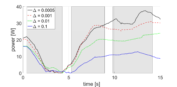
(a) Time history of the consumed power for right front limb

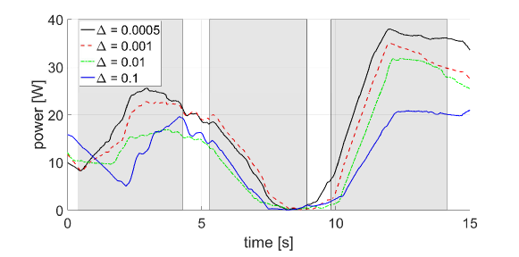
(b) Time history of the consumed power for right middle limb

Figure 7: Time history of the consumed power under the different violation probabilities. The shaded regions are when the robot lifts a specific limb and puts it on the next position, and white regions are when the robot pushes its body up. The figure shows that the consumed power of a particular limb decreases when the limb is in the air, while it increases when the limb is on the wall to generate the normal force on the wall.

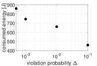
Figure 8: Consumed energy with different $\Delta_{\operatorname{}}$ during $t=0-15$ s

IV-B Climbing on Non-uniform Walls

This scenario demonstrates that the robot designs different trajectories under the different violation probability to climb on walls with varying coefficients of friction. The planned trajectories are shown in Fig. 9. In this example, the robot climbs between two walls where the terrain shown in black is covered by 36-grit sandpapers ($\lambda=2.3$), the terrain shown in green is covered by 80-grit sandpapers ($\lambda=1.1$), and the terrain shown in red is covered by the material with $\lambda=0$ as shown in Fig. 9. The varying coefficients of friction are modeled by a parabola function, which encourages the solver to converge on a solution. In the left panel of Fig. 9, the violation probability $\Delta_{\operatorname{}}$ is 0.1 while in the right panel, the violation probability $\Delta_{\operatorname{}}$ is 0.001 for ${\color[rgb]{0,0,0}M=6}$ and $N=7$.

The left panel of Fig. 9 illustrates that the robot avoids the red area (zero friction) and puts its foot mostly in the black area (high friction), but sometimes also in the green area (low friction) to minimize the trajectory length. In the right panel of Fig. 9, the violation probability is decreased, and the robot footsteps completely remain inside the high friction area. As a result, our proposed NLP-based planner operates the pose and forces together and makes a trade-off between a shorter but more risky trajectory and a longer but safer trajectory. This cannot be achieved if the planner decouples the footstep and force planning, such as in [9]. Fig. 10 shows the trajectory with higher risk bound $\Delta_{\operatorname{}}=0.1$ and compares the foot location at $t=146$ with the foot location with $\Delta_{\operatorname{}}=0.001$ in the hardware experiment. We notice that at $t=146$ s, the foot touches the white area where the coefficient of friction is 0, which never happened with $\Delta_{\operatorname{}}=0.001$. Since the robot only controls its body orientation based on IMU feedback and does not control its linear position, the implemented trajectory does not strictly follow the planned one. We observe that lower risk bound is beneficial in this situation to avoid failure since it compensates for the tracking error by the imperfect controller.

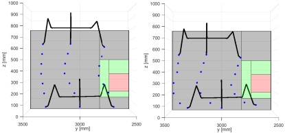
Figure 9: Side view of planned footsteps on non-uniform walls under: left $\Delta_{\operatorname{}}=0.1$, right $\Delta_{\operatorname{}}=0.001$. In the left panel, the robot puts its feet on low and high friction terrain by taking a high risk bound. In the right panel, the robot puts its feet only on high friction terrain.

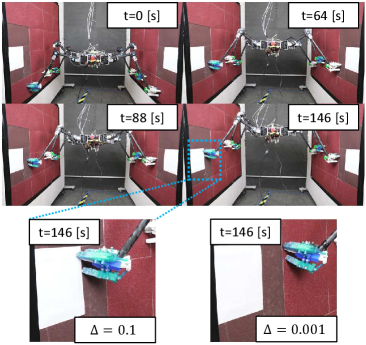
Figure 10: Snapshots of climbing experiments on non-uniform walls under the different violation probabilities

IV-C Climbing with Less Stable Gait: Tripod Gait

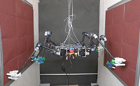
Figure 11: Climbing with tripod gait. Left: A planned trajectory of the tripod gait under $\Delta_{\operatorname{}}=0.4$. Red arrows indicate the reaction forces from the walls. Right: A snapshot of climbing experiments with the tripod gait under $\Delta_{\operatorname{}}=0.4$.

In this scenario, we demonstrate that the robot can conduct a tripod gait, when it lifts three legs simultaneously, by setting the violation probability much higher. Before installing the gripper on the current six-limbed robot, it was almost infeasible to climb on the walls with the tripod gait because of the torque limits of the motors. With the grippers installed, however, the robot has a greater chance to climb on the walls with a tripod gait. If we set $\Delta=0$, the problem is infeasible since the constraints under the worst-case uncertainty are conservative. This result would be equivalent to the results of other robust algorithm such as [12], where the optimization-based robust approach with the worst-case uncertainty is proposed. However, by utilizing the chance constraints and increasing the violation probability, the planner generates a feasible solution. In our trial, we set the violation probability $\Delta_{\operatorname{}}=0.4$ for ${\color[rgb]{0,0,0}M=6}$ and $N=3$, and allowed the robot to climb on a wall covered by 36-grit sandpapers. The planner investigates 4 critical instants: 2 instants after the robot lifts three limbs, and 2 instants after the robot places them down and pushes its body. The planned trajectory is illustrated in the left panel of Fig. 11. As shown in the right under the condition, the robot succeeded in climbing on the walls with the tripod gait and its climbing velocity was 2.5 cm/s, which is three times faster than the one leg gait.

V CONCLUSION and FUTURE WORKS

In this paper, we presented a motion planning algorithm for limbed robots with stochastic gripping forces. Our proposed planner exploits NLP to simultaneously plan a pose and force with guaranteed bounded risk. Maximum gripping forces are modeled as a Gaussian distribution by employing the GP, which provides the planner with the mean and the covariance information to formulate the chance constraints. We showed that under our planning framework, the robot demonstrates rich - sometimes drastically different - behaviors, including planning a risky but energy-efficient motion versus a safe but exhausting motion, avoiding danger zones like low friction environments, and choosing fast but less stable motions (i.e., a tripod gait) based on the different violation probabilities $\Delta_{\operatorname{}}$ in hardware experiments.

The current limitation in this work is that the actual probability of failure is not strictly equal to pre-defined $\Delta_{\operatorname{}}$ because other sources of uncertainty exist, such as sensor noises. In future work, we will extend our planner to take into consideration these sources.

References

- [1] T. Bretl, S. Lall, J. C. Latombe, and S. Rock, “Multi-step motion planning for free-climbing robots,” in Algorithmic Foundations of Robotics VI, Springer, pp. 59–74, 2004.
- [2] A. Shkolnik, M. Levashov, I. R. Manchester, and R. Tedrake, “Bounding on rough terrain with the LittleDog robot,” Int. J. Rob. Res., vol. 30, issue 2, pp. 192–215, 2011.
- [3] A. K. Valenzuela, “Mixed-integer convex optimization for planning aggressive motions of legged robots over rough terrain,” PhD Thesis, Massachusetts Institute of Technology, 2016.
- [4] A. W. Winkler, C. D. Bellicoso, M. Hutter, and J. Buchli, “Gait and trajectory optimization for legged systems through phase-based end-effector parameterization,” IEEE Robot. Autom. Lett., vol. 3, no. 3, pp. 1560–1567, 2018.
- [5] B. Aceituno-Cabezas et al., “Simultaneous contact, gait, and motion planning for robust multilegged locomotion via mixed-integer convex optimization,” IEEE Robot. Autom. Lett., vol. 3, no 3, pp. 2531–2538, 2018.
- [6] A. W. Winkler et al., “Fast trajectory optimization for legged robots using vertex-based ZMP constraints,” IEEE Robot. Autom. Lett., vol. 2, no 4, pp. 2201-2208, 2017.
- [7] A. D. Prete and N. Mansard, “Robustness to joint-torque-tracking errors in task-space inverse dynamics,” IEEE Trans. Robot., vol. 32, no 5, pp. 1091-1105, 2016.
- [8] M. Brandão et al., “Material recognition CNNs and hierarchical planning for biped robot locomotion on slippery terrain,” in Proc. 2016 IEEE-RAS Conf. Humanoid Robots, pp. 81–88, 2016.
- [9] X. Lin, J. Zhang, J. Shen, G. Fernandez, and D. W. Hong, "Optimization based motion planning for multi-limbed vertical climbing robots," in Proc. 2019 IEEE/RSJ Conf. Intell. Robots Syst., pp. 1918-1925, 2019.
- [10] S. Wang, H. Jiang, and M. R Cutkosky, “Design and modeling of linearly-constrained compliant spines for human-scale locomotion on rocky surfaces,” Int. J. Rob. Res., vol. 36, issue 9, pp. 985-999, 2017.
- [11] H. Jiang, S. Wang, and M. R Cutkosky, "Stochastic models of compliant spine arrays for rough surface grasping,“ Int. J. Rob. Res., vol. 37, no. 7, pp.669-687, 2018.
- [12] O. S. Tas and C. Stiller, “Limited visibility and uncertainty aware motion planning for automated driving,” in Proc. 2018 IEEE Intelligent Vehicles Symposium, pp. 1171–1178, 2018.
- [13] L. Blackmore and M. Ono, ”Convex chance constrained predictive control without sampling,” in Proc. AIAA Guid. Navigat. Control Conf., 2009.
- [14] M. Ono and B. C. Williams, “An efficient motion planning algorithm for stochastic dynamic systems with constraints on probability of failure,” in Proc. 2008 AAAI Conf. Artif. Intell., pp. 3427–3432, 2008.
- [15] M. Ono, M. Pavone, Y. Kuwata, and J. B. Balaram, “Chance-constrained dynamic programming with application to risk-aware robotic space exploration,” Autom. Robots, vol. 39, no. 4, pp. 555–571, 2015.
- [16] X. Lin, H. Krishnan, Y. Su, and D. W. Hong, “Multi-limbed robot vertical two wall climbing based on static indeterminacy modeling and feasibility region analysis,” in Proc. 2018 IEEE/RSJ Conf. Intell. Robots Syst., pp. 4355-4362, 2018.
- [17] A. Pashkevich, A. Klimchik, and D. Chablat, “Enhanced stiffness modeling of manipulators with passive joints, Mechanism and machine theory,” Mech. Mach. Theory , vol. 46, pp. 662-679, 2011.
- [18] C. Rasmussen and C. Williams, “Gaussian processes for machine learning,” MIT press, vol. 1, 2006.
- [19] K. Nagaoka et al., "Passive spine gripper for free-climbing robot in extreme terrain," IEEE Robot. Autom. Lett., vol. 3, no 3, pp. 1765- 1770, 2018.
- [20] A. Asbeck et al., "Scaling hard vertical surfaces with compliant microspine arrays," Int. J. Rob. Res., vol. 25, no. 12, pp. 1165-1179, 2006.
- [21] K. Autumn et al., "Frictional adhesion: a new angle on gecko attachment," J. Exp. Biol., vol. 209, issue 18, pp. 3569-3579, 2006.
- [22] R. Fletcher, “Practical methods of optimization,” NY: John Wiley Sons, vol. 2, 1981.
- [23] A. Waechter and L. T. Biegler, “On the implementation of an interior-point filter line-search algorithm for large-scale nonlinear programming,” Mathematical Programming , vol. 106, no. 1, pp. 25–57, 2006.
- [24] J. A. E. Andersson et al., “CasADi – A software framework for nonlinear optimization and optimal control,” Mathematical Programming, vol. 11, no. 1, pp. 1-36, 2019.