Continuation Newton methods with the residual trust-region time-stepping scheme for nonlinear equations

Abstract

For nonlinear equations, the homotopy methods (continuation methods) are popular in engineering fields since their convergence regions are large and they are quite reliable to find a solution. The disadvantage of the classical homotopy methods is that their computational time is heavy since they need to solve many auxiliary nonlinear systems during the intermediate continuation processes. In order to overcome this shortcoming, we consider the special explicit continuation Newton method with the residual trust-region time-stepping scheme for this problem. According to our numerical experiments, the new method is more robust and faster to find the required solution of the real-world problem than the traditional optimization method (the built-in subroutine fsolve.m of the MATLAB environment) and the homotopy continuation methods (HOMPACK90 and NAClab). Furthermore, we analyze the global convergence and the local superlinear convergence of the new method.

1 Introduction

In engineering fields, we often need to solve the equilibrium state of the differential equation Liao2012 ; MM1990 ; Robertson1966 ; VL1994 as follows:

$$\frac{dx}{dt}=F(x),\;x(t_{0})=x_{0}.$$ (1)

That is to say, it requires to solve the following system of nonlinear equations:

$$F(x)=0,$$ (2)

where $F:\;\Re^{n}\to\Re^{n}$ is a vector function. For the nonlinear system (2), there are many popular traditional optimization methods CGT2000 ; DS2009 ; Higham1999 ; NW1999 and the classical homotopy continuation methods AG2003 ; Doedel2007 ; OR2000 ; WSMMW1997 to solve it.

For the traditional optimization methods such as the trust-region methods More1978 ; Yuan1998 ; Yuan2015 and the line search methods Kelley2003 ; Kelley2018 , the solution $x^{\ast}$ of the nonlinear system (2) is found via solving the following equivalent nonlinear least-squares problem

$$\min_{x\in\Re^{n}}f(x)=\frac{1}{2}\|F(x)\|^{2},$$ (3)

where $\|\cdot\|$ denotes the Euclidean vector norm or its induced matrix norm. Generally speaking, the traditional optimization methods based on the merit function (3) are efficient for the large-scale problems since they have the local superlinear convergence near the solution $x^{\ast}$ CGT2000 ; NW1999 .

However, the line search methods and the trust-region methods are apt to stagnate at a local minimum point $x^{\ast}$ of problem (3), when the Jacobian matrix $J(x^{\ast})$ of $F(x^{\ast})$ is singular or nearly singular, where $J(x)={\partial F(x)}/{\partial x}$ (see p. 304, NW1999 ). Furthermore, the termination condition

$$\|\nabla f(x_{k})\|=\|J(x_{k})^{T}F(x_{k})\|<\epsilon,$$ (4)

may lead these methods to early stop far away from the local minimum $x^{\ast}$. It can be illustrated as follows. We consider

$$F(x)=Ax=0,\hskip 5.69054ptA=\begin{bmatrix}1&0\\ 0&10^{-6}\end{bmatrix}.$$ (5)

It is not difficult to know that the linear system (5) has a unique solution $x^{\ast}=(0,\,0)$. If we set $\epsilon=10^{-6}$, the traditional optimization methods will early stop far away from $x^{\ast}$ provided that $x_{k}=(0,\;c),\;c<10^{6}$.

For the classical homotopy methods, the solution $x^{\ast}$ of the nonlinear system (2) is found via constructing the following homotopy function

$$H(x,\,\lambda)=(1-\lambda)G(x)+\lambda F(x),$$ (6)

and attempting to trace an implicitly defined curve $\lambda(t)\in H^{-1}(0)$ from the starting point $(x_{0},\,0)$ to a solution $(x^{\ast},\,1)$ by the predictor-corrector methods AG2003 ; Doedel2007 , where the zero point of the artificial smooth function $G(x)$ is known. Generally speaking, the homotopy continuation methods are more reliable than the merit-function methods and they are very popular in engineering fields Liao2012 . The disadvantage of the classical homotopy methods is that they require significantly more function and derivative evaluations, and linear algebra operations than the merit-function methods since they need to solve many auxiliary nonlinear systems during the intermediate continuation processes.

In order to overcome this shortcoming of the traditional homotopy methods, we consider the special continuation method based on the following Newton flow AS2015 ; Branin1972 ; Davidenko1953 ; Tanabe1979

$$\frac{dx(t)}{dt}=-J(x)^{-1}F(x),\;x(t_{0})=x_{0},$$ (7)

and construct a special ODE method with the new time-stepping scheme based on the trust-region updating strategy to follow the trajectory of the Newton flow (7). Consequently, we obtain its steady-state solution $x^{\ast}$, i.e. the required solution $x^{\ast}$ of the nonlinear system (2).

The rest of this article is organized as follows. In the next section, we consider the explicit continuation Newton method with the trust-region updating strategy for nonlinear equations. In section 3, we prove the global convergence and the local superlinear convergence of the new method under some standard assumptions. In section 4, some promising numerical results of the new method are also reported, in comparison to the traditional trust-region method (the built-in subroutine fsolve.m of the MATLAB environment MATLAB ; More1978 ) and the classical homotopy continuation methods (HOMOPACK90 WSMMW1997 and NAClab LLT2008 ; ZL2013 ; Zeng2019 ). Finally, some conclusions and the future work are discussed in section 5. Throughout this article, we assume that $F(\cdot)$ exists the zero point $x^{\ast}$.

2 Continuation Newton methods

In this section, based on the trust-region updating strategy, we construct a new time-stepping scheme for the continuation Newton method to follow the trajectory of the Newton flow and obtain its steady-state solution $x^{\ast}$.

2.1 The continuous Newton flow

If we consider the damped Newton method with the line search strategy for the nonlinear system (2) Kelley2003 ; NW1999 , we have

$$x_{k+1}=x_{k}-\alpha_{k}J(x_{k})^{-1}F(x_{k}).$$ (8)

We denote $o(\alpha)$ as the higher-order infinitesimal of $\alpha$, that is to say,

$$\lim_{\alpha\to 0}\frac{o(\alpha)}{\alpha}=0.$$

In equation (8), if we let $x_{k}=x(t_{k})$, $x_{k+1}=x(t_{k}+\alpha_{k})+o(\alpha_{k})$ and $\alpha_{k}\to 0$, we obtain the continuous Newton flow (7). Actually, if we apply an iteration with the explicit Euler method HNW1993 ; SGT2003 to the continuous Newton flow (7), we also obtain the damped Newton method (8). Since the Jacobian matrix $J(x)$ may be singular, we reformulate the continuous Newton flow (7) as the more general formula:

$$-J(x)\frac{dx(t)}{dt}=F(x),\hskip 5.69054ptx(t_{0})=x_{0}.$$ (9)

The continuous Newton flow (9) is an old method and can be backtracked to Davidenko’s work Davidenko1953 in 1953. After that, it was investigated by Branin Branin1972 , Deuflhard et al PHP1975 , Tanabe Tanabe1979 and Kalaba et al KZHH1977 in 1970s, and applied to nonlinear boundary problems by Axelsson and Sysala AS2015 recently. The continuous and even growing interest in this method originates from its some nice properties. One of them is that the solution $x(t)$ of the continuous Newton flow converges to the steady-state solution $x^{\ast}$ from any initial point $x_{0}$, as described by the following property 1.

Property 1

(Branin Branin1972 and Tanabe Tanabe1979 ) Assume that $x(t)$ is the solution of the continuous Newton flow (9), then $f(x(t))=\|F(x)\|^{2}$ converges to zero when $t\to\infty$. That is to say, for every limit point $x^{\ast}$ of $x(t)$, it is also a solution of the nonlinear system (2). Furthermore, every element $F^{i}(x)$ of $F(x)$ has the same convergence rate $e^{-t}$ and $x(t)$ can not converge to the solution $x^{\ast}$ of the nonlinear system (2) on the finite interval when the initial point $x_{0}$ is not a solution of the nonlinear system (2).

Proof.  Assume that $x(t)$ is the solution of the continuous Newton flow (9), then we have

$$\frac{d}{dt}\left(e^{t}F(x)\right)=e^{t}J(x)\frac{dx(t)}{dt}+e^{t}F(x)=0.$$

Consequently, we obtain

$$F(x(t))=F(x_{0})e^{-t}.$$ (10)

From equation (10), it is not difficult to know that every element $F^{i}(x)$ of $F(x)$ converges to zero with the linear convergence rate $e^{-t}$ when $t\to\infty$. Thus, if the solution $x(t)$ of the continuous Newton flow (9) belongs to a compact set, it has a limit point $x^{\ast}$ when $t\to\infty$, and this limit point $x^{\ast}$ is also a solution of the nonlinear system (2).

If we assume that the solution $x(t)$ of the continuous Newton flow (9) converges to the solution $x^{\ast}$ of the nonlinear system (2) on the finite interval $(0,\,T]$, from equation (10), we have

$$F(x^{\ast})=F(x_{0})e^{-T}.$$ (11)

Since $x^{\ast}$ is a solution of the nonlinear system (2), we have $F(x^{\ast})=0$. By substituting it into equation (11), we obtain

$$F(x_{0})=0.$$

Thus, it contradicts the assumption that $x_{0}$ is not a solution of the nonlinear system (2). Consequently, the solution $x(t)$ of the continuous Newton flow (9) can not converge to the solution $x^{\ast}$ of the nonlinear system (2) on the finite interval. ∎

Remark 1

The inverse $J(x)^{-1}$ of the Jacobian matrix $J(x)$ can be regarded as the preconditioner of $F(x)$ such that the solution elements $x^{i}(t)\,(i=1,\,2,\ldots,n)$ of the continuous Newton flow (7) have the roughly same convergence rates and it mitigates the stiff property of the ODE (7) (the definition of the stiff problem can be found in HW1996 and references therein). This property is very useful since it makes us adopt the explicit ODE method to follow the trajectory of the Newton flow.

Actually, if we consider $F(x)=Ax$, from the ODE (9), we have

$$A\frac{dx}{dt}=-Ax,\;x(0)=x_{0}.$$ (12)

By integrating the linear ODE (12), we obtain

$$x(t)=e^{-t}x_{0}.$$ (13)

From equation (13), we know that the solution $x(t)$ of the ODE (12) linearly converges to zero with the same rate $e^{-t}$ when $t$ tends to infinity.

2.2 Continuation Newton methods

From subsection 2.1, we know that the solution $x(t)$ of the continuous Newton flow (9) has the nice global convergence property. On the other hand, when the Jacobian matrix $J(x)$ is singular or nearly singular, the ODE (9) is the system of differential-algebraic equations (DAEs) and its trajectory can not be efficiently followed by the general ODE method such as the backward differentiation formulas (the built-in subroutine ode15s.m of the MATLAB environment AP1998 ; BCP1996 ; HW1996 ; MATLAB ; SGT2003 ). Thus, we need to construct the special method to handle this problem. Furthermore, we expect that the new method has the global convergence as the homotopy continuation methods and the fast convergence rate near the solution $x^{\ast}$ as the merit-function methods. In order to achieve these two aims, we construct the special continuous Newton method with the new step size $\alpha_{k}=\Delta t_{k}/(1+\Delta t_{k})$ and the time step $\Delta t_{k}$ is adaptively adjusted by the trust-region updating strategy for problem (9).

Firstly, we apply the implicit Euler method to the continuous Newton flow (9) AP1998 ; BCP1996 , then we obtain

$$J(x_{k+1}){(x_{k+1}-x_{k})}/{\Delta t_{k}}=-F(x_{k+1}).$$ (14)

The scheme (14) is an implicit method. Thus, it needs to solve a system of nonlinear equations at every iteration. To avoid solving the system of nonlinear equations, we replace $J(x_{k+1})$ with $J(x_{k})$ and substitute $F(x_{k+1})$ with its linear approximation $F(x_{k})+J(x_{k})(x_{k+1}-x_{k})$ in equation (14). Thus, we obtain the continuation Newton method as follows:

$$J(x_{k})s_{k} =-({\Delta t_{k}}/{(1+\Delta t_{k})})F(x_{k}),$$ (15)

$$x_{k+1} =x_{k}+s_{k}.$$ (16)

Remark 2

The explicit continuation Newton method (15)-(16) is similar to the damped Newton method (8) if we let $\alpha_{k}=\Delta t_{k}/(1+\Delta t_{k})$ in equation (15). However, from the view of the ODE method, they are different. The damped Newton method (8) is obtained by the explicit Euler method applied to the continuous Newton flow (9), and its time step $\alpha_{k}$ is restricted by the numerical stability HW1996 ; SGT2003 . That is to say, the large time step $\alpha_{k}$ can not be adopted in the steady-state phase. The explicit continuation Newton method (15)-(16) is obtained by the implicit Euler method and its linear approximation applied to the continuous Newton flow (9), and its time step $\Delta t_{k}$ is not restricted by the numerical stability for the linear test equation $dx/dt=-\lambda x,\;\lambda>0$. Therefore, the large time step $\Delta t_{k}$ can be adopted in the steady-state phase for the explicit continuation Newton method (15)-(16), and it mimics the Newton method near the steady-state solution $x^{\ast}$ such that it has the fast local convergence rate. The most of all, the new time step $\alpha_{k}=\Delta t_{k}/(\Delta t_{k}+1)$ is favourable to adopt the trust-region updating strategy for adaptively adjusting the time step $\Delta t_{k}$ such that the explicit continuation Newton method (15)-(16) accurately follows the trajectory of the continuous Newton flow in the transient-state phase and achieves the fast convergence rate near the steady-sate solution $x^{\ast}$.

For the real-world problem, the Jacobian matrix $J(x)$ may be singular, which arises from the physical property. For example, for the chemical kinetic reaction problem (1), the elements of $x(t)$ represent the reaction concentrations and they must satisfy the linear conservation law Logan1996 . A system is called to satisfy the linear conservation law (Shampine1998 , or p. 35, SGT2003 ), if there is a constant vector $c\neq 0$ such that

$$c^{T}x(t)=c^{T}x(0)$$ (17)

holds for all $t\geq 0$. If there exists a constant vector $c$ such that

$$c^{T}F(x)=0,\quad\forall x\in\Re^{n},$$ (18)

we have

$$c^{T}J(x)=0,\quad\forall x\in\Re^{n}.$$ (19)

From equation (19), we know that the Jacobian matrix $J(x)$ is singular. For this case, the solution $x(t)$ of the ODE (1) satisfies the linear conservation law (17).

For the isolated singularity of the Jacobian matrix $J(x)$, there are some efficient approaches to handle this problem Griewank1985 . Here, since the singularity set of the Jacobian matrix $J(x)$ may be connected, we adopt the regularization technique Hansen1994 ; KK1998 to modify the explicit continuation Newton method (15)-(16) as follows:

$$\left(\mu_{k}I-J(x_{k})\right)s_{k}^{P} =F(x_{k}),$$ (20)

$$s_{k} =({\Delta t_{k}}/{(1+\Delta t_{k})})s_{k}^{P},$$ (21)

$$x_{k+1} =x_{k}+s_{k},$$ (22)

where $\mu_{k}$ is a small positive number. In order to achieve the fast convergence rate near the solution $x^{\ast}$, the regularization continuation Newton method (20)-(22) is required to approximate the Newton method $x_{k+1}=x_{k}-J(x_{k})^{-1}F(x_{k})$ near the solution $x^{\ast}$ DM1974 . Thus, we select the regularization parameter $\mu_{k}$ as follows:

$$\mu_{k}=\begin{cases}c_{\epsilon},\;\text{if}\;\Delta t_{k}\leq 1/c_{\epsilon},\\ 1/\Delta t_{k},\;\text{others},\end{cases}$$ (23)

where $c_{\epsilon}$ is a small positive constant such as $c_{\epsilon}=10^{-6}$ in practice.

It is not difficult to verify that the regularization continuation Newton method (20)-(22) preserves the linear conservation law (17) if it exists a constant vector $c\in\Re^{n}$ such that $c^{T}F(x)=0,\;\forall x\in\Re^{n}$. Actually, from $c^{T}F(x)=0$, we have $c^{T}J(x)=0$. Therefore, from equations (20)-(22), we obtain

$$c^{T}x_{k+1}=c^{T}x_{k}+c^{T}s_{k}=c^{T}x_{k}+\frac{1}{\mu_{k}}c^{T}\left(\frac{\Delta t_{k}}{1+\Delta t_{k}}F(x_{k})+J(x_{k})s_{k}\right)=c^{T}x_{k}.$$ (24)

That is to say, the regularization continuation Newton method (20)-(22) preserves the linear conservation law (17).

2.3 The residual trust-region time-stepping scheme

Another issue is how to adaptively adjust the time-stepping size $\Delta t_{k}$ at every iteration. A popular way to control the time-stepping size is based on the trust-region technique CGT2000 ; Deuflhard2004 ; Higham1999 ; LLT2007 ; Luo2010 . For this time-stepping scheme, it needs to select suitable a merit function and construct an approximation model of the merit function. Here, we adopt the residual $\|F(x)\|$ as the merit function and adopt $\|F(x_{k})+J(x_{k})s_{k}\|$ as the approximation model of $\|F(x_{k}+s_{k})\|$. Thus, according to the following ratio:

$$\rho_{k}=\frac{\|F(x_{k})\|-\|F(x_{k}+s_{k})\|}{\|F(x_{k})\|-\|F(x_{k})+J(x_{k})s_{k})\|},$$ (25)

we enlarge or reduce the time step $\Delta t_{k}$ at every iteration. A particular adjustment strategy is given as follows:

$$\Delta t_{k+1}=\begin{cases}\gamma_{1}\Delta t_{k},&{\text{if}\;\left|1-\rho_{k}\right|\leq\eta_{1},}\\ \Delta t_{k},&{\text{else if}\;\eta_{1}<\left|1-\rho_{k}\right|<\eta_{2},}\\ \gamma_{2}\Delta t_{k},&{\text{others},}\end{cases}$$ (26)

where the constants are selected as $\gamma_{1}=2,\;\gamma_{2}=0.5,\;\eta_{1}=0.25,\;\eta_{2}=0.75$ according to our numerical experiments.

Remark 3

This new time-stepping scheme based on the trust-region updating strategy has some advantages compared to the traditional line search strategy Luo2005 . If we use the line search strategy and the damped Newton method (8) to track the trajectory $z(t)$ of the continuous Newton flow (9), in order to achieve the fast convergence rate in the steady-state phase, the time step size $\alpha_{k}$ of the damped Newton method is tried from 1 and reduced by half with many times at every iteration. Since the linear model $F(x_{k})+J(x_{k})s_{k}$ may not approximate $F(x_{k}+s_{k})$ well in the transient-state phase, the time step size $\alpha_{k}$ will be small. Consequently, the line search strategy consumes the unnecessary trial steps in the transient-state phase. However, the selection scheme of the time step size based on the trust-region updating strategy (25)-(26) can overcome this shortcoming.

According to the above discussions, we give the detailed implementation of the regularization continuation Newton method with the residual trust-region time-stepping scheme for nonlinear equations in Algorithm 1.

Algorithm 1 Continuation Newton methods with the residual trust-region time-stepping scheme (The CNMTr method)

0:    Function $F:\;\Re^{n}\to\Re^{n}$, the initial point $x_{0}$   (optional), and the tolerance $\epsilon$   (optional).

0:    An approximation solution $x^{\ast}$ of nonlinear equations.

1:  Set the default $x_{0}=\text{ones}(n,\;1)$ and $\epsilon=10^{-6}$ when $x_{0}$ or $\epsilon$ is not provided by the calling subroutine.

2:  Initialize the parameters: $\eta_{a}=10^{-6},\;\eta_{1}=0.25,\;\gamma_{1}=2,\;\eta_{2}=0.75,\;\gamma_{2}=0.5,\;\text{maxit}=400$.

3:  Set $\Delta t_{0}=10^{-2}$, flag_success_trialstep = 1, $\text{itc}=0,\;k=0$.

4:  Evaluate $F_{k}=F(x_{k})$ and $J_{k}=J(x_{k})$. Compute the residual $Res_{0}=\|F(x_{0})\|_{\infty}$.

5:  while (itc $<$ maxit) do

6:     if (flag_success_trialstep == 1) then

7:        Set itc = itc + 1.

8:        Compute $\text{Res}_{k}=\|F_{k}\|_{\infty}$.

9:        if ($\text{Res}_{k}<\epsilon$) then

10:           break;

11:        end if

12:        Solve the linear system (20) to obtain the Newton step $s_{k}^{P}$.

13:     end if

14:     Compute $s_{k}={\Delta t_{k}}/{(1+\Delta t_{k})}\,s_{k}^{P}$.

15:     Set $x_{k+1}=x_{k}+s_{k}$.

16:     Evaluate $F(x_{k+1})$.

17:     if $\|F(x_{k})\|<\|F(x_{k})+J(x_{k})s_{k}\|$ then

18:        $\rho_{k}=-1$;

19:     else

20:        Compute the ratio $\rho_{k}$ from equation (25).

21:     end if

22:     Adjust the time-stepping size $\Delta t_{k+1}$ according to the trust-region updating strategy (26).

23:     if $(\rho_{k}\geq\eta_{a})$ then

24:        Accept the trial point $x_{k+1}$. Set flag_success_trialstep = 1.

25:     else

26:        Set $x_{k+1}=x_{k}$, $F_{k+1}=F_{k}$, $s_{k+1}^{P}=s_{k}^{P}$, flag_success_trialstep = 0.

27:     end if

28:     Set $k\longleftarrow k+1$.

29:  end while

3 Convergence analysis

In this section, we discuss some theoretical properties of Algorithm 1. Firstly, we estimate the lower bound of the predicted reduction $\|F(x_{k})\|-\|F(x_{k})+J(x_{k})s_{k}\|$, which is similar to the estimate of the trust-region method for the unconstrained optimization problem Powell1975 .

Lemma 1

Assume that it exists a positive constant $m$ such that

$$\|J(x_{k})y\|\geq m\|y\|,\;\forall y\in\Re^{n},\;k=0,\,1,\,2,\,\ldots.$$ (27)

Furthermore, we suppose that $s_{k}$ is the solution of the regularization continuation Newton method (20)-(22), where the regularization parameter $\mu_{k}$ defined by equation (23) and the constant $c_{\epsilon}$ satisfy $\mu_{k}\leq c_{\epsilon}<0.5m$. Then, we have the following estimation

$$\|F(x_{k})\|-\|F(x_{k})+J(x_{k})s_{k}\|\geq c_{r}\,\|F(x_{k})\|\,{\Delta t_{k}}/{(1+\Delta t_{k})},$$ (28)

where the positive constant $c_{r}$ satisfies $0<c_{r}<1$.

Proof.  From equations (20)-(21), we have

$$-J(x_{k})s_{k}+\mu_{k}s_{k}=({\Delta t_{k}}/{(1+\Delta t_{k})})F(x_{k}).$$ (29)

Thus, from equation (29), we obtain

$$\|J(x_{k})s_{k}+F(x_{k})\|=\left\|\mu_{k}s_{k}+{F(x_{k})}/{(1+\Delta t_{k})}\right\|$$

$$\quad=\left\|\mu_{k}({\Delta t_{k}}/{(1+\Delta t_{k})})\,(-J(x_{k})+\mu_{k}I)^{-1}F(x_{k})+{F(x_{k})}/{(1+\Delta t_{k})}\right\|$$

$$\quad\leq({1}/{(1+\Delta t_{k})})\,\left(\Delta t_{k}\left\|\left(-{J(x_{k})}/{\mu_{k}}+I\right)^{-1}\right\|+1\right)\|F(x_{k})\|.$$ (30)

According to the definition of the induced matrix norm GV2013 , we have

$$\left\|\left(-{J(x_{k})}/{\mu_{k}}+I\right)^{-1}\right\|=\max_{z\neq 0}{\left\|\left(-{J(x_{k})}/{\mu_{k}}+I\right)^{-1}z\right\|}/{\|z\|}$$

$$=\max_{y\neq 0}\frac{\|y\|}{\left\|\left(-{J(x_{k})}/{\mu_{k}}+I\right)y\right\|}=\frac{1}{\min_{\|y\|=1}\left\|\left(-{J(x_{k})}/{\mu_{k}}+I\right)y\right\|}.$$ (31)

On the other hand, when $\|y\|=1$, from the nonsingular assumption (27) of matrix $J(x_{k})$, we have

$$\left\|\left(-{J(x_{k})}/{\mu_{k}}+I\right)y\right\|=\left\|-{J(x_{k})y}/{\mu_{k}}+y\right\|$$

$$\hskip 5.69054pt\geq{\|J(x_{k})y\|}/{\mu_{k}}-\|y\|\geq{m}/{\mu_{k}}-1.$$ (32)

Thus, from the assumption $\mu_{k}\leq c_{\epsilon}<0.5m$ and equations (31)-(32), we have

$$\left\|\left(-{J(x_{k})}/{\mu_{k}}+I\right)^{-1}\right\|\leq{\mu_{k}}/{(m-\mu_{k})}\leq{c_{\epsilon}}/{(m-c_{\epsilon})}.$$ (33)

By substituting inequality (33) into inequality (30), we have

$$\|J(x_{k})s_{k}+F(x_{k})\|\leq(\left(1+{c_{\epsilon}\Delta t_{k}}/{(m-c_{\epsilon})}\right)/{(1+\Delta t_{k})})\|F(x_{k})\|.$$

That is to say, we obtain

$$\|F(x_{k})\|-\|F(x_{k})+J(x_{k})s_{k}\|\geq\left(\frac{m-2c_{\epsilon}}{m-c_{\epsilon}}\right)\frac{\Delta t_{k}}{1+\Delta t_{k}}\|F(x_{k})\|.$$ (34)

We set $c_{r}=(m-2c_{\epsilon})/(m-c_{\epsilon})$ in the above inequality (34). Then, we obtain the estimation (28). ∎

In order to prove that the sequence $\{\|F(x_{k})\|\}$ converges to zero when $k$ tends to infinity, we also need to estimate the lower bound of the time step size $\Delta t_{k}$.

Lemma 2

Assume that $F:\;\Re^{n}\to\Re^{n}$ is continuously differentiable and its Jacobian function $J$ is Lipschitz continuous. That to say, it exists a positive number $L$ such that

$$\|J(x)-J(y)\|\leq L\|x-y\|$$ (35)

holds for all $x,\,y\in\Re^{n}$. Furthermore, we suppose that the sequence $\{x_{k}\}$ is generated by Algorithm 1 and the nonsingular condition (27) of matrix $J(x_{k})$ holds. Then, when the regularization parameter $\mu_{k}$ defined by equation (23) and the constant $c_{\epsilon}$ satisfy $\mu_{k}\leq c_{\epsilon}<0.5m$, it exists a positive number $\delta_{\Delta t}$ such that

$$\Delta t_{k}\geq\delta_{\Delta t}>0,\;k=0,\,1,\;2,\dots,$$ (36)

where $\Delta t_{k}$ is adaptively adjusted by formulas (25)-(26).

Proof.  From the Lipschitz continuous assumption (35) of $J(\cdot)$, we have

$$\left\|F(x_{k+1})-F(x_{k})-J(x_{k})s_{k}\right\|=\left\|\int_{0}^{1}J(x_{k}+ts_{k})s_{k}dt-J(x_{k})s_{k}\right\|$$

$$=\left\|\int_{0}^{1}(J(x_{k}+ts_{k})-J(x_{k}))s_{k}dt\right\|\leq\int_{0}^{1}\|(J(x_{k}+ts_{k})-J(x_{k}))s_{k}\|dt$$

$$\leq\int_{0}^{1}\|J(x_{k}+ts_{k})-J(x_{k})\|\|s_{k}\|dt\leq\int_{0}^{1}L\|s_{k}\|^{2}tdt=0.5\,L\|s_{k}\|^{2}.$$ (37)

On the other hand, from equations (20)-(21), we have

$$\|s_{k}\| =({\Delta t_{k}}/{(1+\Delta t_{k})})\left\|\left(-J(x_{k})+\mu_{k}I\right)^{-1}F(x_{k})\right\|$$

$$\leq({\Delta t_{k}}/{(1+\Delta t_{k})})\left\|\left(-J(x_{k})+\mu_{k}I\right)^{-1}\right\|\|F(x_{k})\|.$$ (38)

Similarly to the estimation (33), from the assumption $\mu_{k}\leq c_{\epsilon}<0.5m$ and the nonsingular assumption (27) of $J(x_{k})$, we have

$$\left\|(-J(x_{k})+\mu_{k}I)^{-1}\right\|\leq{1}/{(m-\mu_{k})}\leq{1}/{(m-c_{\epsilon})}.$$ (39)

Thus, from inequalities (37)-(39), we obtain

$$\left\|F(x_{k+1})-F(x_{k})-J(x_{k})s_{k}\right\|\leq\frac{L}{2(m-c_{\epsilon})^{2}}\left(\frac{\Delta t_{k}}{1+\Delta t_{k}}\right)^{2}\|F(x_{k})\|^{2}.$$ (40)

From the definition (25) of $\rho_{k}$, the estimation (34), and inequality (40), we have

$$|\rho_{k}-1|=\left|\frac{\|F(x_{k})\|-\|F(x_{k+1})\|}{\|F(x_{k})\|-\|F(x_{k})+J(x_{k})s_{k}\|}-1\right|$$

$$\hskip 5.69054pt\leq\frac{\|F(x_{k+1})-F(x_{k})-J(x_{k})s_{k}\|}{\|F(x_{k})\|-\|F(x_{k})+J(x_{k})s_{k}\|}\leq\frac{L}{2(m-2c_{\epsilon})^{2}}\left(\frac{\Delta t_{k}}{1+\Delta t_{k}}\right)\|F(x_{k})\|.$$ (41)

According to Algorithm 1, we know that the sequence $\{\|F(x_{k})\|\}$ is monotonically decreasing. Consequently, we have $\|F(x_{k})\|\leq\|F(x_{0})\|,\;k=1,\,2,\,\dots$. We set

$$\bar{\delta}_{\Delta t}\triangleq{2(m-2c_{\epsilon})^{2}\eta_{1}}/{(\|F(x_{0})\|L)}.$$ (42)

Assume that $K$ is the first index such that $\Delta t_{K}\leq\bar{\delta}_{\Delta t}$. Then, from inequalities (41)-(42), we obtain $|\rho_{K}-1|<\eta_{1}$. Consequently, $\Delta t_{K+1}$ will be greater than $\Delta t_{K}$ according to the adaptive adjustment scheme (26). We set $\delta_{\Delta t}=\min\{\Delta t_{K},\bar{\delta}_{\Delta t}\}$. Then, $\Delta t_{k}\geq\delta_{\Delta t}$ holds for all $k=0,\,1,\,2,\,\dots$. ∎

By using the estimation results of Lemma 1 and Lemma 2, we can prove that the sequence $\{\|F(x_{k})\|\}$ converges to zero when $k$ tends to infinity.

Theorem 3.1

Assume that $F:\;\Re^{n}\to\Re^{n}$ is continuously differentiable and its Jacobian function $J$ satisfies the Lipschitz condition (35). Furthermore, we suppose that the sequence $\{x_{k}\}$ is generated by Algorithm 1 and $J(x_{k})$ satisfies the nonsingular assumption (27). Then, when the regularization parameter $\mu_{k}$ defined by equation (23) and the constant $c_{\epsilon}$ satisfy $\mu_{k}\leq c_{\epsilon}<0.5m$, we have

$$\lim_{k\to\infty}\inf\;\|F(x_{k})\|=0.$$ (43)

Proof.  According to Algorithm 1 and inequality (41), we know that there exists an infinite subsequence $\{x_{k_{l}}\}$ such that

$$\frac{\|F(x_{k_{l}})\|-\|F(x_{k_{l}}+s_{k_{l}})\|}{\|F(x_{k_{l}})\|-\|F(x_{k_{l}})+J(x_{k_{l}})s_{k_{l}}\|}\geq\eta_{a},\;l=1,\,2,\,\ldots.$$ (44)

Otherwise, all steps are rejected after a given iteration index, then the time step size $\Delta t_{k}$ will keep decreasing, which contradicts equation (36).

From inequalities (28), (36) and (44), we have

$$\|F(x_{k_{l}})\|-\|F(x_{k_{l}}+s_{k_{l}})\|\geq\frac{\eta_{a}c_{r}\Delta t_{k_{l}}}{(1+\Delta t_{k_{l}})}\|F(x_{k_{l}})\|\geq\frac{\eta_{a}c_{r}\delta_{\Delta t}}{(1+\delta_{\Delta t})}\|F(x_{k_{l}})\|.$$ (45)

Therefore, from equation (45) and $\|F(x_{k+1})\|\leq\|F(x_{k})\|$, we have

$$\|F(x_{0})\|\geq\|F(x_{0})\|-\lim_{k\to\infty}\|F(x_{k})\|=\sum_{k=0}^{\infty}(\|F(x_{k})\|-\|F(x_{k+1})\|)$$

$$\hskip 5.69054pt\geq\sum_{l=0}^{\infty}(\|F(x_{k_{l}})\|-\|F(x_{k_{l}}+s_{k_{l}})\|)\geq\frac{\eta_{a}c_{r}\delta_{\Delta t}}{1+\delta_{\Delta t}}\sum_{l=0}^{\infty}\|F(x_{k_{l}})\|.$$ (46)

Consequently, from inequality (46), we obtain

$$\lim_{k_{l}\to\infty}\|F(x_{k_{l}})\|=0.$$ (47)

That is to say, the result (43) is true. Furthermore, from $\|F(x_{k+1})\|\leq\|F(x_{k})\|$ and equation (47), it is not difficult to know $\lim_{k\to\infty}\|F(x_{k})\|=0$. ∎

Under the nonsingular assumption of $J(x^{\ast})$ and the local Lipschitz continuity (35) of $J(\cdot)$, we analyze the local superlinear convergence rate of Algorithm 1 near the solution $x^{\ast}$ as follows. For convenience, we define the neighbourhood $B_{\delta}(x^{\ast})$ of $x^{\ast}$ as

$$B_{\delta}(x^{\ast})=\{x:\|x-x^{\ast}\|\leq\delta\}.$$

Theorem 3.2

Assume that $F:\;\Re^{n}\to\Re^{n}$ is continuously differentiable and $F(x^{\ast})=0$. Furthermore, we suppose that $J$ satisfies the local Lipschitz continuity (35) around $x^{\ast}$ and the nonsingular condition (27) when $x\in B_{\delta}(x^{\ast})$. Then, when the regularization parameter $\mu_{k}$ defined by equation (23) and the constant $c_{\epsilon}$ satisfy $\mu_{k}\leq c_{\epsilon}<0.5m$, there exists a neighborhood $B_{r}(x^{\ast})$ such that the sequence $\{x_{k}\}$ generated by Algorithm 1 with $x_{0}\in B_{r}(x^{\ast})$ superlinearly converges to $x^{\ast}$.

Proof.  The framework of its proof can be roughly described as follows. Firstly, we prove that the sequence $\{x_{k}\}$ linearly converges to $x^{\ast}$ when $x_{0}$ gets close enough to $x^{\ast}$. Then, we prove $\lim_{k\to\infty}\Delta t_{k}=\infty$. Finally, we prove that the search step $s_{k}$ approximates the Newton step $s_{k}^{N}$. Consequently, the sequence $\{x_{k}\}$ superlinearly converges to $x^{\ast}$.

Firstly, similarly to the estimation (33), from the assumption $\mu_{k}\leq c_{\epsilon}<0.5m$, we obtain

$$\left\|(\mu_{k}I-J(x_{k}))^{-1}\right\|\leq{1}/{(m-c_{\epsilon})},\;\forall x_{k}\in B_{\delta}(x^{\ast}),\;k=0,\,1,\,2,\ldots.$$ (48)

We denote $e_{k}=x_{k}-x^{\ast}$. From equations (20)-(21), we have

$$e_{k+1} =e_{k}+s_{k}=e_{k}+\frac{\Delta t_{k}}{1+\Delta t_{k}}\left(\mu_{k}I-J(x_{k})\right)^{-1}(F(x_{k})-F(x^{\ast}))$$

$$=e_{k}+\frac{\Delta t_{k}}{1+\Delta t_{k}}\left(\mu_{k}I-J(x_{k})\right)^{-1}\int_{0}^{1}J(x^{\ast}+te_{k})e_{k}dt.$$ (49)

By rearranging the above equation (49), we obtain

$$e_{k+1}=\frac{1}{1+\Delta t_{k}}e_{k}+\frac{\Delta t_{k}}{1+\Delta t_{k}}\left(\mu_{k}I-J(x_{k})\right)^{-1}\int_{0}^{1}\left(J(x^{\ast}+te_{k})-J(x_{k})+\mu_{k}I\right)e_{k}dt.$$

By using the Lipschitz continuous assumption (35) of $J(\cdot)$, the estimation (48), and the assumption $\mu_{k}\leq c_{\epsilon}<0.5m$, we have

$$\|e_{k+1}\|\leq{\|e_{k}\|}/{(1+\Delta t_{k})}$$

$$\hskip 5.69054pt+({\Delta t_{k}}/{(1+\Delta t_{k})})\left\|\left(\mu_{k}I-J(x_{k})\right)^{-1}\right\|\int_{0}^{1}\left(\left\|J(x^{\ast}+te_{k})-J(x_{k})\right\|+\mu_{k}\right)\|e_{k}\|dt$$

$$\hskip 5.69054pt\leq{\|e_{k}\|}/{(1+\Delta t_{k})}+({\Delta t_{k}}/{((1+\Delta t_{k})(m-\mu_{k}))})\left(\mu_{k}+0.5L\|e_{k}\|\right)\|e_{k}\|$$

$$\hskip 5.69054pt=\frac{1+\frac{1}{m-\mu_{k}}\left(\mu_{k}+0.5L\|e_{k}\|\right){\Delta t_{k}}}{1+\Delta t_{k}}\|e_{k}\|\leq\frac{1+\frac{1}{m-c_{\epsilon}}\left(c_{\epsilon}+0.5L\|e_{k}\|\right){\Delta t_{k}}}{1+\Delta t_{k}}\|e_{k}\|.$$ (50)

We denote

$$q_{k}\triangleq\frac{1+\left(c_{\epsilon}+0.5L\|e_{k}\|\right){\Delta t_{k}}/({m-c_{\epsilon}})}{1+\Delta t_{k}},$$ (51)

and select $x_{0}\in B_{\delta}(x^{\ast})$ to satisfy

$$\|e_{0}\|<{(m-2c_{\epsilon})}/{L}.$$ (52)

We set $r=\min\{\delta,(m-2c_{\epsilon})/L\}$. When $x_{0}\in B_{r}(x^{\ast})$, from equations (50)-(52) and the assumption $c_{\epsilon}<0.5m$, by induction, we have

$$\|e_{k+1}\|\leq q_{k}\|e_{k}\|,\;q_{k}<\frac{1+{0.5\Delta t_{k}\,m}/{(m-c_{\epsilon})}}{1+\Delta t_{k}}<1,\;k=0,\,1,\,\ldots.$$ (53)

It is not difficult to know that $f(t)\triangleq(1+\alpha t)/(1+t)$ is monotonically decreasing when $0\leq\alpha<1$. Thus, from the estimation (36) of the time step size $\Delta t_{k}$ and inequality (53), we obtain

$$\|e_{k+1}\|\leq q_{k}\|e_{k}\|\leq q\|e_{k}\|,\;q\triangleq\frac{1+{0.5\delta_{\Delta t}m}/{(m-c_{\epsilon})}}{1+\delta_{\Delta t}}<1.$$

Therefore, we have

$$\|e_{k+1}\|\leq q^{k}\|e_{0}\|\to 0,\;\text{when}\;k\to\infty.$$ (54)

That is to say, we obtain $\lim_{k\to\infty}x_{k}=x^{\ast}$.

Secondly, from equations (20)-(21) and inequality (48), we have

$$\|s_{k}\| =({\Delta t_{k}}/{(1+\Delta t_{k})})\left\|(-J(x_{k})+\mu_{k}I)^{-1}F(x_{k})\right\|$$

$$\leq\frac{\Delta t_{k}}{1+\Delta t_{k}}\left\|(-J(x_{k})+\mu_{k}I)^{-1}\right\|\|F(x_{k})\|\leq\frac{1}{m-c_{\epsilon}}\frac{\Delta t_{k}}{1+\Delta t_{k}}\|F(x_{k})\|.$$ (55)

Similarly to the estimation (41), from the definition (25) of $\rho_{k}$, inequalities (34) and (55), we have

$$|\rho_{k}-1| =\left|\frac{\|F(x_{k})\|-\|F(x_{k+1})\|}{\|F(x_{k})\|-\|F(x_{k})+J(x_{k})s_{k}\|}-1\right|$$

$$\leq\frac{0.5L}{(m-2c_{\epsilon})^{2}}\left(\frac{\Delta t_{k}}{1+\Delta t_{k}}\right)\|F(x_{k})\|\leq\frac{0.5L}{(m-2c_{\epsilon})^{2}}\|F(x_{k})\|.$$ (56)

Since $\{\|F(x_{k})\|\}$ is monotonically decreasing and $\lim_{k\to\infty}x_{k}=x^{\ast},\;F(x^{\ast})=0$, we can select a sufficiently large number $K$ such that

$$\|F(x_{k})\|\leq\frac{2\eta_{1}(m-2c_{\epsilon})^{2}}{L},\;\text{when}\;k\geq K.$$ (57)

From inequalities (56)-(57), we have

$$|\rho_{k}-1|\leq\eta_{1},\;\text{when}\;k\geq K.$$

This means $\Delta t_{k+1}=\gamma_{1}\Delta t_{k}$ when $k\geq K$, according to the time-stepping scheme (26). That is to say, we have

$$\lim_{k\to\infty}\Delta t_{k}=\infty.$$ (58)

Finally, since $\lim_{k\to\infty}\Delta t_{k}=\infty$, we can select a sufficiently large number $K_{\mu}$ such that $1/\Delta t_{k}<c_{\epsilon}$ when $k\geq K_{\mu}$. Consequently, from the definition (23) of the regularization parameter $\mu_{k}$, we obtain $\mu_{k}=1/\Delta t_{k}$ when $k\geq K_{\mu}$. By substituting it into inequality (50), we have

$$\frac{\|e_{k+1}\|}{\|e_{k}\|}\leq\frac{1}{1+\Delta t_{k}}+\frac{\Delta t_{k}}{1+\Delta t_{k}}\frac{1}{m-\mu_{k}}\left(\mu_{k}+0.5L\|e_{k}\|\right)$$

$$\hskip 5.69054pt=\frac{1}{1+\Delta t_{k}}+\frac{\Delta t_{k}}{1+\Delta t_{k}}\frac{1}{m-{1}/{\Delta t_{k}}}\left(1/{\Delta t_{k}}+0.5L\|e_{k}\|\right),\;\text{when}\;k\geq K_{\mu}.$$ (59)

From equations (54) and (58), we know $\lim_{k\to\infty}\|e_{k}\|=0$ and $\lim_{k\to\infty}\Delta t_{k}=\infty$, respectively. Therefore, by combining them with inequality (59), we obtain

$$\lim_{k\to\infty}\frac{\|e_{k+1}\|}{\|e_{k}\|}=0.$$

That is to say, the sequence $\{x_{k}\}$ superlinearly converges to $x^{\ast}$. ∎

For the real-world problem, the singularity of $J(x)$ may arise from the linear conservation law such as the conservation of mass or the conservation of charge Luo2009 ; Shampine1998 ; Shampine1999 ; SGT2003 . In the rest of this section, we analyze convergence properties of Algorithm 1 when $J(x)$ is singular. Similarly to the standard assumption of the nonlinear dynamical system, we suppose that $J(\cdot)$ satisfies the one-sided Lipschitz condition (see p. 303, Deuflhard2004 or p. 180, HW1996 ) as follows:

$$y^{T}J(x)y\leq-\nu\|y\|^{2},\;\text{for}\;y\in{S}_{c}=\left\{y|c^{T}y=0\right\},\;\nu>0,$$ (60)

where the constant vector $c$ satisfies $c^{T}F(x)=0,\;\forall x\in\Re^{n}$. The positive number $\nu$ is called the one-sided Lipschitz constant. Under the assumption of the one-sided Lipschitz condition (60), we know that matrix $(\mu I-J(x))$ is nonsingular when $\mu>0$. We state it as the following property 2.

Property 2

Assume that $J(\cdot)$ satisfies the one-sided Lipschitz condition (60). Then, matrix $(\mu I-J(x))$ is nonsingular when $\mu>0$, and the solution $s_{k}$ of equations (20)-(21) satisfies $c^{T}s_{k}=0$.

Proof.  We prove it by contradiction. If we assume that matrix $(\mu I-J(x))$ is singular, there exists a nonzero vector $y$ such that

$$(\mu I-J(x))y=0.$$ (61)

Consequently, from the assumption $c^{T}F(x)=0$, we have

$$c^{T}y=c^{T}(J(x)y)/\mu=\left(c^{T}J(x)\right)y/\mu=0.$$

Thus, from the one-sided Lipschitz condition (60) and $\mu>0,\;\nu>0$, we obtain

$$y^{T}(\mu I-J(x))y=\mu\|y\|^{2}-y^{T}J(x)y\geq(\mu+\nu)\|y\|^{2}>0,$$

which contradicts the assumption (61). Therefore, matrix $(\mu I-J(x))$ is nonsingular.

From equations (20)-(21), we have

$$\left(\mu_{k}I-J(x_{k})\right)s_{k}=({\Delta t_{k}}/{(1+\Delta t_{k})})F(x_{k}).$$ (62)

By combining it with the assumption $c^{T}F(x_{k})=0$, we obtain

$$c^{T}(\mu_{k}I-J(x_{k}))s_{k}=({\Delta t_{k}}/{(1+\Delta t_{k})})c^{T}F(x_{k})=0.$$ (63)

Therefore, by substituting $c^{T}J(x_{k})=0$ into equation (63), we have

$$\mu_{k}c^{T}s_{k}=c^{T}J(x_{k})s_{k}=\left(c^{T}J(x_{k})\right)s_{k}=0.$$ (64)

That is to say, we obtain $c^{T}s_{k}=0$. ∎

Similarly to the estimation (28) of $\|F(x_{k})\|-\|F(x_{k})+J(x_{k})s_{k}\|$ for the nonsingular Jacobian matrix $J(x_{k})$, we also have its lower-bounded estimation when $J(x_{k})$ is singular, $k=0,\,1,\,2,\,\ldots$.

Lemma 3

Assume that $J(x_{k})$ satisfies the one-sided Lipschitz condition (60) and $s_{k}$ is the solution of equations (20)-(22). Then, we have

$$\|F(x_{k})\|-\|F(x_{k})+J(x_{k})s_{k}\|\geq c_{s}({\Delta t_{k}}/{(1+\Delta t_{k})})\|F(x_{k})\|,$$ (65)

where the positive constant $c_{s}$ satisfies $0<c_{s}<1$.

Proof.  From Property 2, we know that matrix $(\mu I-J(x_{k}))$ is nonsingular and $s_{k}$ satisfies $c^{T}s_{k}=0$. From equations (20)-(21) and the Cauchy-Schwartz inequality $|x^{T}y|\leq\|x\|\|y\|$, we have

$$\mu_{k}\|s_{k}\|^{2}-s_{k}^{T}J(x_{k})s_{k}={s_{k}^{T}F(x_{k})\Delta t_{k}}/{(1+\Delta t_{k})}\leq({\Delta t_{k}}/{(1+\Delta t_{k})})\|s_{k}\|\|F(x_{k})\|.$$ (66)

By substituting one-sided Lipschitz condition (60) into equation (66), we obtain

$$(\mu_{k}+\nu)\|s_{k}\|^{2}\leq\mu_{k}\|s_{k}\|^{2}-s_{k}^{T}J(x_{k})s_{k}\leq({\Delta t_{k}}/{(1+\Delta t_{k})})\|s_{k}\|\|F(x_{k})\|.$$

Consequently, we have

$$\|s_{k}\|\leq\frac{1}{\mu_{k}+\nu}\frac{\Delta t_{k}}{1+\Delta t_{k}}\|F(x_{k})\|.$$ (67)

From equations (20)-(21) and (67), we have

$$\|F(x_{k})+J(x_{k})s_{k}\|=\left\|\mu_{k}s_{k}+\frac{1}{1+\Delta t_{k}}F(x_{k})\right\|\leq\mu_{k}\|s_{k}\|+\frac{1}{1+\Delta t_{k}}\|F(x_{k})\|$$

$$\hskip 5.69054pt\leq\frac{\mu_{k}}{\mu_{k}+\nu}\frac{\Delta t_{k}}{1+\Delta t_{k}}\|F(x_{k})\|+\frac{1}{1+\Delta t_{k}}\|F(x_{k})\|.$$ (68)

From the definition (23) of the parameter $\mu_{k}$, we know $\mu_{k}\leq c_{\epsilon}$. By substituting it into inequality (68), we obtain

$$\|F(x_{k})\|-\|F(x_{k})+J(x_{k})s_{k}\|\geq\frac{\nu}{\mu_{k}+\nu}\frac{\Delta t_{k}}{1+\Delta t_{k}}\|F(x_{k})\|$$

$$\quad\geq\frac{\nu}{c_{\epsilon}+\nu}\frac{\Delta t_{k}}{1+\Delta t_{k}}\|F(x_{k})\|.$$ (69)

We set $c_{s}=\nu/(c_{\epsilon}+\nu)$. Then, from equation (69), we obtain the estimation (65). ∎

Similarly to the lower-bounded estimation (36) of the time step size $\Delta t_{k}$ for the nonsingular Jacobian matrix $J(x_{k})$, we also have its lower-bounded estimation when $J(x_{k})$ is singular, $k=0,\,1,\,2,\,\ldots$.

Lemma 4

Assume that $F:\;\Re^{n}\to\Re^{n}$ is continuously differentiable and $J(\cdot)$ satisfies the Lipschitz continuity (35) and the one-sided Lipschitz condition (60). The sequence $\{x_{k}\}$ is generated by Algorithm 1. Then, there exists a positive $\delta_{s}$ such that

$$\Delta t_{k}\geq\delta_{s}>0,\;k=1,\;2,\ldots,$$ (70)

where $\Delta t_{k}$ is adaptively updated by the trust-region updating strategy (25)-(26).

Proof.  From the Lipschitz continuity (35) of $J(\cdot)$, we have

$$\left\|F(x_{k+1})-F(x_{k})-J(x_{k})s_{k}\right\|=\left\|\int_{0}^{1}(J(x_{k}+ts_{k})-J(x_{k}))s_{k}dt\right\|$$

$$\hskip 5.69054pt\leq\int_{0}^{1}\|J(x_{k}+ts_{k})-J(x_{k})\|\|s_{k}\|dt\leq\int_{0}^{1}L\|s_{k}\|^{2}tdt=0.5L\|s_{k}\|^{2}.$$ (71)

By substituting the estimation (67) of $s_{k}$ into inequality (71), we obtain

$$\left\|F(x_{k+1})-F(x_{k})-J(x_{k})s_{k}\right\|\leq\frac{0.5L}{(\mu_{k}+\nu)^{2}}\left(\frac{\Delta t_{k}}{1+\Delta t_{k}}\right)^{2}\|F(x_{k})\|^{2}.$$ (72)

Thus, from the definition (25) of $\rho_{k}$, inequalities (69) and (72), we obtain

$$|\rho_{k}-1|=\left|\frac{\|F(x_{k})\|-\|F(x_{k+1})\|}{\|F(x_{k})\|-\|F(x_{k})+J(x_{k})s_{k}\|}-1\right|\leq\frac{\|F(x_{k+1})-F(x_{k})-J(x_{k})s_{k}\|}{\|F(x_{k})\|-\|F(x_{k})+J(x_{k})s_{k}\|}$$

$$\quad\leq\frac{L}{2\nu(\mu_{k}+\nu)}\left(\frac{\Delta t_{k}}{1+\Delta t_{k}}\right)\|F(x_{k})\|\leq\frac{L}{2\nu^{2}}\left(\frac{\Delta t_{k}}{1+\Delta t_{k}}\right)\|F(x_{k})\|.$$ (73)

According to Algorithm 1, we know that the sequence $\{\|F(x_{k})\|\}$ is monotonically decreasing. Consequently, we have $\|F(x_{k})\|\leq\|F(x_{0})\|$,   $k=1,\,2,\,\dots$. We set

$$\bar{\delta}_{s}={2\nu^{2}\eta_{1}}/{(\|F(x_{0})\|L)}.$$ (74)

If we assume that $K$ is the first index such that $\Delta t_{K}\leq\bar{\delta}_{s}$, then, from inequalities (73)-(74), we obtain $|\rho_{K}-1|<\eta_{1}$. Consequently, $\Delta t_{K+1}$ will be greater than $\Delta t_{K}$ according to the time-stepping scheme (26). Set $\delta_{s}=\min\{\Delta t_{K},\bar{\delta}_{s}\}$. Then, we have $\Delta t_{k}\geq\delta_{s},\;k=0,\,1,\,2,\,\dots$. ∎

Now, from Lemma 3 and Lemma 4, we know that the sequence $\{\|F(x_{k})\|\}$ converges to zero when $k$ tends to infinity and its proof is similar to the proof of Theorem 3.1. We state it as the following theorem 3.3 and omit its proof.

Theorem 3.3

Assume that $F:\;\Re^{n}\to\Re^{n}$ is continuously differentiable and its Jacobian function $J(\cdot)$ satisfies the Lipschitz continuity (35) and the one-sided Lipschitz condition (60). The sequence $\{x_{k}\}$ is generated by Algorithm 1. Then, we have

$$\lim_{k\to\infty}\inf\;\|F(x_{k})\|=0.$$ (75)

Theorem 3.4

Assume that $F:\;\Re^{n}\to\Re^{n}$ is continuously differentiable and its Jacobian function $J(\cdot)$ satisfies the Lipschitz continuity (35) and the one-sided Lipschitz condition (60). Furthermore, we suppose that the sequence $\{x_{k}\}$ is generated by Algorithm 1 and its subsequence $\{x_{k_{i}}\}$ converges to $x^{\ast}$. Then, the sequence $\{x_{k}\}$ superlinearly converges to $x^{\ast}$.

Proof.  The framework of its proof can be roughly described as follows. Firstly, we prove $\lim_{k\to\infty}\Delta t_{k}=\infty$. Then, we prove that the sequence $\{x_{k}\}$ linearly converges to $x^{\ast}$. Finally, we prove that the search step $s_{k}$ approximates the Newton step $s_{k}^{N}$. Consequently, the sequence $\{x_{k}\}$ superlinearly converges to $x^{\ast}$.

From Property 2, we know that matrix $(\mu I-J(x_{k}))$ is nonsingular and $s_{k}$ satisfies $c^{T}s_{k}=0$, where the constant vector $c$ satisfies $c^{T}F(x)=0$ for all $x\in\Re^{n}$ and $s_{k}$ is the solution of equations (20)-(21).

Firstly, we prove that there exists an index $K$ such that $\Delta t_{k}$ will be enlarged at every iteration when $k\geq K$. Consequently, we have $\lim_{k\to\infty}\Delta t_{k}=\infty$. From the lower-bounded estimation (69) of $F(x_{k})-F(x_{k}+s_{k})$ and inequality (73), we have

$$|\rho_{k}-1|=\left|\frac{\|F(x_{k})\|-\|F(x_{k+1})\|}{\|F(x_{k})\|-\|F(x_{k})+J(x_{k})s_{k}\|}-1\right|$$

$$\quad\leq\frac{L}{2\nu(\mu_{k}+\nu)}\left(\frac{\Delta t_{k}}{1+\Delta t_{k}}\right)\|F(x_{k})\|\leq\frac{L}{2\nu^{2}}\|F(x_{k})\|.$$ (76)

Since the subsequence $\{x_{k_{i}}\}$ converges to $x^{\ast}$, there exists an index $K_{F}$ such that

$$\|F(x_{K_{F}})\|\leq{2\eta_{1}\nu^{2}}/{L}.$$ (77)

Furthermore, according to Algorithm 1, we know that the sequence $\{\|F(x_{k})\|\}$ is monotonically decreasing. Consequently, we have $\|F(x_{k})\|\leq\|F(x_{K_{F}})\|$ when $k\geq K_{F}$. Thus, from inequalities (76)-(77), we have

$$|\rho_{k}-1|\leq\eta_{1},\;\text{when}\;k\geq K_{F}.$$ (78)

Consequently, according to the time-stepping scheme (26), we know that $\Delta t_{k+1}=\gamma_{1}\Delta t_{k}$ when $k\geq K_{F}$. Therefore, we obtain $\lim_{k\to\infty}\Delta t_{k}=\infty$.

Secondly, we prove that the sequence $\{x_{k}\}$ linearly converges to $x^{\ast}$ as follows. We denote

$$e_{k}=x_{k}-x^{\ast}.$$ (79)

From equations (20)-(21) and (79), we have

$$e_{k+1}=e_{k}+s_{k}=e_{k}+({\Delta t_{k}}/{(1+\Delta t_{k})})\left(\mu_{k}I-J(x_{k})\right)^{-1}F(x_{k}).$$ (80)

By rearranging inequality (80), we obtain

$$\left(\mu_{k}I-J(x_{k})\right)e_{k+1}=\left(\mu_{k}I-J(x_{k})\right)e_{k}+({\Delta t_{k}}/{(1+\Delta t_{k})})(F(x_{k})-F(x^{\ast}))$$

$$\quad=\mu_{k}e_{k}-{J(x_{k})e_{k}}/{\Delta t_{k}}+({\Delta t_{k}}/{(1+\Delta t_{k})})\int_{0}^{1}\left(J(x^{\ast}+te_{k})-J(x_{k})\right)e_{k}dt.$$ (81)

Since $c^{T}s_{k}$ = 0 and the subsequence $\{x_{k_{i}}\}_{i=1}^{+\infty}$ converges to $x^{\ast}$, from equation (80), we have

$$c^{T}e_{k+1}=c^{T}e_{k}+c^{T}s_{k}=c^{T}e_{k}=\cdots=c^{T}e_{k_{i}}\to 0,\;\text{when}\;i\to\infty.$$

That is to say, we have $c^{T}e_{k}=0,\;k=0,\,1,\,\ldots$. Thus, from the one-sided Lipschitz condition (60) and the Cauchy-Schwartz inequality $|x^{T}y|\leq\|x\|\,\|y\|$, we have

$$\|e_{k+1}\|\left\|\left(\mu_{k}I-J(x_{k})\right)e_{k+1}\right\|\geq e_{k+1}^{T}\left(\mu_{k}I-J(x_{k})\right)e_{k+1}$$

$$=\mu_{k}e^{T}_{k+1}e_{k+1}-e^{T}_{k+1}J(x_{k})e_{k+1}\geq(\mu_{k}+\nu)\|e_{k+1}\|^{2}.$$ (82)

By rearranging inequality (82), we obtain

$$\|e_{k+1}\|\leq{\left\|\left(\mu_{k}I-J(x_{k})\right)e_{k+1}\right\|}/{(\mu_{k}+\nu)}.$$ (83)

From the continuity of $J$ at $x^{\ast}$, there exists the positive constants $M$ and $\epsilon$ such that

$$\|J(x)\|\leq M\;\text{when}\;\|x-x^{\ast}\|<\epsilon.$$

Since the subsequence $\{x_{k_{i}}\}$ converges to $x^{\ast}$, there exists $K_{1}$ such that $\|x_{K_{1}}-x^{\ast}\|<\epsilon$. By combining it with $\lim_{k\to\infty}\Delta t_{k}=\infty$, we can select a sufficiently large number $K_{2}$ such that $\Delta t_{K_{2}}\geq 4M/\nu$ and $\|e_{K_{2}}\|\leq 0.5\nu/L$. We set $K=\max\{K_{1},\,K_{2}\}$.

From equation (81) and the Lipschitz continuity (35), we have

$$\|(\mu_{K}I-J(x_{K}))e_{K+1}\|\leq\mu_{K}\|e_{K}\|+{\|J(x_{K})\|\|e_{K}\|}/{\Delta t_{K}}$$

$$\hskip 5.69054pt+\int_{0}^{1}\|J(x^{\ast}+te_{K})-J(x_{K})\|\|e_{K}\|dt\,{\Delta t_{K}}/{(1+\Delta t_{K})}$$

$$\hskip 5.69054pt\leq\left(\mu_{K}+{M}/{\Delta t_{K}}\right)\|e_{K}\|+\int_{0}^{1}L\|e_{K}\|^{2}tdt\leq\left(\mu_{K}+{M}/{\Delta t_{K}}+0.5L\|e_{K}\|\right)\|e_{K}\|.$$

By combining it with inequality (83), $\Delta t_{K}\geq(4M)/\nu$, and $\|e_{K}\|\leq\nu/(2L)$, we obtain

$$\|e_{K+1}\|\leq\frac{\mu_{K}+{M}/{\Delta t_{K}}+0.5L\|e_{K}\|}{\mu_{K}+\nu}\|e_{K}\|\leq\frac{\mu_{K}+0.5\nu}{\mu_{K}+\nu}\|e_{K}\|<\|e_{K}\|<\epsilon.$$ (84)

Therefore, by induction, we obtain

$$\|e_{k+1}\|\leq\frac{\mu_{k}+{M}/{\Delta t_{k}}+0.5L\|e_{k}\|}{\mu_{k}+\nu}\|e_{k}\|\leq\frac{\mu_{k}+0.5\nu}{\mu_{k}+\nu}\|e_{k}\|,\;\text{when}\;k\geq K.$$ (85)

Furthermore, from the definition (23), we know that $\mu_{k}<c_{\epsilon}$. By substituting it into inequality (85), we have

$$\|e_{k+1}\|\leq q\|e_{k}\|\leq\cdots\leq q^{(k-K+1)}\|e_{K}\|,\;q\triangleq\frac{c_{\epsilon}+1/2\nu}{c_{\epsilon}+\nu}<1,\;\text{when}\;k\geq K.$$

Consequently, we obtain $\lim_{k\to\infty}\|e_{k}\|=0$.

Finally, we prove that the sequence $\{x_{k}\}$ superlinearly converges to $x^{\ast}$. Since $\lim_{k\to\infty}\Delta t_{k}=\infty$, we can select a sufficiently large number $K_{\mu}$ such that $1/\Delta t_{k}<c_{\epsilon}$ when $k\geq K_{\mu}$. Thus, from the definition (23) of the regularization parameter $\mu_{k}$, we know $\mu_{k}=1/\Delta t_{k}$ when $k\geq K_{\mu}$. By substituting it into equation (85), we obtain

$$\frac{\|e_{k+1}\|}{\|e_{k}\|} \leq\frac{\mu_{k}+{M}/{\Delta t_{k}}+0.5L\|e_{k}\|}{\mu_{k}+\nu}=\frac{{1}/{\Delta t_{k}}+{M}/{\Delta t_{k}}+0.5L\|e_{k}\|}{{1}/{\Delta t_{k}}+\nu}.$$ (86)

Consequently, from $\lim_{k\to\infty}\Delta t_{k}=\infty$, $\lim_{k\to\infty}\|e_{k}\|=0$, and equation (86), we have $\lim_{k\to\infty}{\|e_{k+1}\|}/{\|e_{k}\|}=0$. That is to say, the sequence $\{x_{k}\}$ superlinearly converges to $x^{\ast}$. ∎

4 Numerical Experiments

In this section, for some real-world equilibrium problems and the classical test problems of nonlinear equations, we test the performance of Algorithm 1 (CNMTr) and compare it with the trust-region method (the built-in subroutine fsolve.m of the MATLAB environment MATLAB ; More1978 ) and the homotopy methods (HOMPACK90 WSMMW1997 , and NAClab LLT2008 ; ZL2013 ; Zeng2019 ).

HOMPACK90 WSMMW1997 is a classical homotopy method implemented by fortran 90 for nonlinear equations and it is very popular in engineering fields. Another state-of-the-art homotopy method is the built-in subroutine psolve.m of the NAClab environment LLT2008 ; ZL2013 . Since psolve.m only solves the polynomial systems, we replace psolve.m with its subroutine GaussNewton.m (the Gauss-Newton method) for non-polynomial systems. Therefore, we compare these two homotopy methods with Algorithm 1, too.

We collect $26$ test problems of nonlinear equations, some of which come from the equilibrium problems of chemical reactions HW1996 ; KLH1982 ; Robertson1966 ; VL1994 , and some of which come from the classical test problems Deuflhard2004 ; DS2009 ; LUL1994 ; MGH1981 ; NW1999 . Their simple descriptions are given by Table 1. Their dimensions vary from $1$ to $3000$. The Jacobian matrix $J(\cdot)$ of $F(\cdot)$ is singular for some test problems. The codes are executed by a HP Pavilion notebook with an Intel quad-core CPU. The termination condition is given by

$$\|F(x^{it})\|_{\infty}\leq 10^{-12}.$$ (87)

The numerical results are arranged in Table 3 and Table 2. The number of iterations of CNMTr and fsolve is illustrated by Figure 1. The computational time of these four methods (CNMTr, HOMPACK90, fsolve and NAClab) is illustrated by Figure 2. From Table 3 and Table 2, we find that CNMTr performs well for those test problems. However, the trust-region method (fsolve) and the classical homotopy methods (HOMPACK90 and NAClab) fail to solve some problems, which especially come from the real-world problems with the non-isolated singular Jacobian matrices such as examples $1,\,2,\,3,\,4,\,6,\,21,\,23$. Furthermore, from Figures 1 and 2, we also find that CNMATr has the same fast convergence property as the traditional optimization method (fsolve).

Table 1: Test problems.

Problems	dimension	problem descriptions
Exam 1	$n=3$	Robertson problem, an autocatalytic reaction HW1996 ; Robertson1966
Exam 2	$n=4$	E5, the chemical pyrolysis HW1996
Exam 3	$n=20$	The pollution problem VL1994
Exam 4	$n=5$	The stability problem of an aircraft (p. 279, NW1999 )
Exam 5	$n=1$	$F(x)=\sin(5x)-x$ (p. 279, NW1999 )
Exam 6	$n=2$	$e^{x^{2}+y^{2}}-3=0$, $x+y-\sin\big{(}3(x+y)\big{)}=0$ (p. 149, Deuflhard2004 )
Exam 7	$n=2$	$x=0,\;-2y=0$
Exam 8	$n=3000$	Extended Rosenbrock function (p. 362, DS2009 or MGH1981 )
Exam 9	$n=3000$	Extended Powell singular function (p. 362, DS2009 or MGH1981 )
Exam 10	$n=3000$	Trigonometric function (p. 362, DS2009 or MGH1981 )
Exam 11	$n=3$	Helical valley function (p. 362, DS2009 )
Exam 12	$n=4$	Wood function (p. 362, DS2009 )
Exam 13	$n=3000$	Extended Cragg and Levy function LUL1994
Exam 14	$n=3000$	Singular Broyden problem LUL1994
Exam 15	$n=10$	The tridiagonal system LUL1994
Exam 16	$n=10$	The discrete boundary-value problem LUL1994
Exam 17	$n=100$	Broyden tridiagonal problem LUL1994
Exam 18	$n=5$	The asymptotic boundary value problem PHP1975
Exam 19	$n=3$	The box problem MGH1981
Exam 20	$n=2$	$f_{1}(x)=x_{1}^{2}+x_{2}^{2}-2$, $f_{2}(x)=e^{x_{1}-1}+x_{2}^{2}-2$ (p.149, DS2009 )
Exam 21	$n=2$	Powell badly scaled function MGH1981
Exam 22	$n=2$	Chemical equilibrium problem 1 KLH1982
Exam 23	$n=6$	Chemical equilibrium problem 2 KLH1982
Exam 24	$n=10$	Brown almost linear function MGH1981
Exam 25	$n=3000$	$a=2*\text{ones}(n,1),\;b=\text{ones}((n-1),1)$, $A=\text{diag}(a,1)+\text{diag}(b,1)+\text{diag}(b,-1)$, $Ax-\lambda x=0,\;x^{T}x=1$
Exam 26	$n=3000$	$a=\text{ones}(n,1),\;b=\text{ones}((n-1),1),\;c=2*b$, $A=\text{diag}(a,1)+\text{diag}(b,1)+\text{diag}(c,-1)$, $Ax-\lambda x=0,\;x^{T}x=1$

Table 2: Numerical results.

Exam	CNMTr		HOMPACK90		fsolve		NAClab (psolve)
	CPU (s)	$\|F(x^{it})\|_{\infty}$	CPU (s)	$\|F(x^{it})\|_{\infty}$	CPU (s)	$\|F(x^{it})\|_{\infty}$	CPU (s)	$\|F(x^{it})\|_{\infty}$
1	7.46E-02	4.87E-13	6.31E-01	5.01E-04 (failed)	2.52E-01	1.64E-07	6.84E-01	0 (failed)
2	2.55E-02	9.86E-14	1.09	3.06 (failed)	3.57E-02	1.39E-12 (far sol.)	7.55E-01	4.27E-20 (failed)
3	1.39E-02	9.61E-14	1.02	3.12 (failed)	3.32E-02	9.24E-05 (far sol.)	1.42	0 (failed)
4	1.71E-02	1.17E-15	7.94E-01	0.74 (failed)	1.34E-03	1.93 (failed)	1.35	1.40E+01 (failed)
5	2.98E-02	4.66E-15	5.87E-01	2.60E-12	4.67E-02	5.51E-01 (failed)	1.36	1.96 (failed)
6	3.01E-02	1.11E-16	5.49E-01	1.34E-02 (failed)	2.87E-02	3.44E-15	3.43E-01	4.39 (failed)
7	1.18E-02	3.05E-13	7.52E-01	0	1.36E-02	2.34E-09	2.85E-01	0
8	1.24E+01	3.91E-13	4.21E+02	5.12E-13	8.64E+02	3.20E-13	3.65E+04	7.12E-12
9	2.07E+01	4.10E-13	4.83E+02	6.84E-12	3.55E+02	7.50E-13	3.97E+04	5.21E-13
10	1.94E+01	4.05E-13	5.31E+02	6.31E-15	3.85E+03	6.75 (failed)	4.02E+03	1.20E+04 (failed)
11	4.37E-02	2.58E-13	8.37E-01	2.15E-14	1.69E-02	1.39E-17	4.39E-01	9.90E+02 (failed)
12	1.24E-01	6.77E-13	7.53E-01	8.94E-13	2.07E-01	5.25E-01 (failed)	8.62E-01	6.02E-12
13	4.30E+01	9.58E-13	6.03E+02	9.68E-13	6.91E+02	4.57E-01 (failed)	4.13E+03	4.84E+08 (failed)
14	1.87E+01	6.31E-13	5.91E+02	8.41E-13	4.12E+02	1.48E-06	4.10E+04	8.13E-12
15	3.80E-02	1.42E-14	8.06E-01	3.84E-14	1.99E-02	5.72E-13	4.71E+02	5.18E-13
16	4.67E-02	2.44E-14	2.94	6.57E-14	1.16E-02	6.76E-13	9.20E-01	4.15E-13
17	1.30	6.17E-13	3.54E+01	5.71E-13	2.51E-02	8.88E-16	9.13E+01	3.16E-12
18	1.40E-02	3.81E-16	2.09	6.14E-16	8.02E-03	7.19E-12	7.74E-01	1 (failed)
19	2.07E-02	5.84E-15	2.54	6.58E-12	8.13E-03	4.96E-13	5.45E-01	0
20	6.57E-03	2.66E-15	5.28	5.14E-13	1.09E-02	2.22E-16	3.51E-01	8.53 (failed)
21	1.23E-03	8.77E-15	7.53E-01	1.22E-02 (failed)	5.29E-02	3.55E-05	4.17E-01	1 (failed)
22	5.58E-03	0	7.79E-01	0	6.73E-02	2.73 (failed)	5.41E-01	0
23	1.62E-02	4.48E-13	4.92	1.09E+02 (failed)	4.84E-02	1.05E+02 (failed)	8.31E-01	5.47E+14 (failed)
24	5.30E-02	1.24E-14	7.63E-01	6.26E-13	9.83E-03	4.23E-12	9.00E-01	2.22E-16
25	7.94E+02	6.09E-13	4.87E+02	4.13E-13	3.91E+03	3.55E-15	4.07E+04	1.45E-12
26	1.31E+03	2.30E-13	9.12E+02	6.14E-12	7.77E+03	5.55E-16	7.09E+04	6.14E-12

Table 3: Statistical results.

	CNMTr	HOMPACK90	fsolve	NAClab
number of failed problems	0	7	9	13
number of the minimum time	19	0	7	0

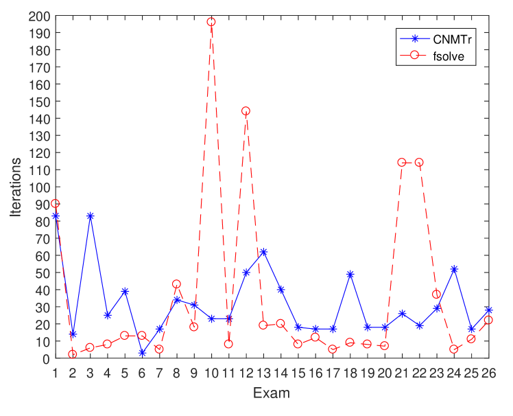
Figure 1: The number of iterations.

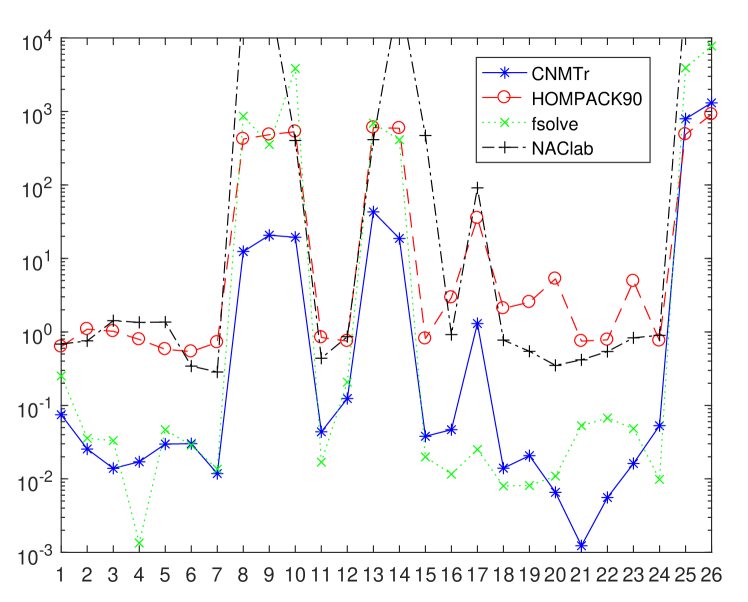
Figure 2: The computational time.

5 Conclusions

In this article, we consider the continuation Newton method with the new time-stepping scheme (CNMTr) based on the trust-region updating strategy. We also analyze its local and global convergence for the nonsingular Jacobian and singular Jacobian problems. Finally, for some classical test problems, we compare it with the classical homotopy methods (HOMPACK90 and psolve.m) and the traditional optimization method (fsolve.m). Numerical results show that CNMTr is more robust and faster than the traditional optimization method. From our point of view, the continuation Newton method with the trust-region updating strategy (Algorithm 1) is worth investigating further as a special continuation method. We have also extended it to the linear programming problem LY2021 , the unconstrained optimization problem LXLZ2021 and the underdetermined system of nonlinear equations LX2021 . The promising results are reported for those problems therein.

Acknowledgments   This work was supported in part by Grant 61876199 from National Natural Science Foundation of China, and Grant YJCB2011003HI from the Innovation Research Program of Huawei Technologies Co., Ltd.. The authors are grateful to two anonymous referees for their helpful comments and suggestions.

References

- (1) Allgower, E.L., Georg, K.: Introduction to Numerical Continuation Methods, SIAM, Philadelphia (2003)
- (2) Ascher, U.M., Petzold, L.R.: Computer Methods for Ordinary Differential Equations and Differential-Algebraic Equations, SIAM, Philadelphia (1998)
- (3) Axelsson, O., Sysala, S.: Continuation Newton methods. Comput. Math. Appl. 70, 2621-2637 (2015)
- (4) Branin, F.H.: Widely convergent method for finding multiple solutions of simultaneous nonlinear equations. IBM J. Res. Dev. 16, 504-521 (1972)
- (5) Brenan, K.E., Campbell, S.L., L. R. Petzold, L.R.: Numerical solution of initial-value problems in differential-algebraic equations, SIAM, Philadelphia (1996)
- (6) Conn, A.R., Gould, N., Toint, Ph.L: Trust-Region Methods, SIAM, Philadelphia (2000)
- (7) Davidenko, D.F.: On a new method of numerical solution of systems of nonlinear equations (in Russian). Dokl. Akad. Nauk SSSR 88, 601-602 (1953)
- (8) Deuflhard, P.: Newton Methods for Nonlinear Problems: Affine Invariance and Adaptive Algorithms, Springer, Berlin (2004)
- (9) Deuflhard, P., Pesch, H.J., Rentrop, P.: A modified continuation method for the numerical solution of nonlinear two-point boundary value problems by shooting techniques. Numer. Math. 26, 327-343 (1975)
- (10) Dennis, J.E, Schnabel, R.B: Numerical Methods for Unconstrained Optimization and Nonlinear Equations, SIAM, Philadelphia (1996)
- (11) Dennis, J.E, Moré, J.J.: A characterization of superlinear convergence and its application to quasi-Newton methods. Math. Comput. 28, 549-560 (1974)
- (12) Doedel, E.J.: Lecture notes in numerical analysis of nonlinear equations. in: Krauskopf, B., Osinga, H.M., Galán-Vioque, J. (Eds.): Numerical Continuation Methods for Dynamical Systems, pp. 1-50, Springer, Berlin (2007)
- (13) Golub, G.H, Van Loan, C.F.: Matrix Computation (4th ed.), The John Hopkins University Press, Baltimore (2013)
- (14) Griewank, A.: On solving nonlinear equations with simple singularities or nearly singular solutions. SIAM Rev. 27, 537-563 (1985)
- (15) Hairer, E., Nørsett, S.P., G. Wanner, G.: Solving Ordinary Differential Equations I, Nonstiff Problems (2nd ed.), Springer, Berlin (1993)
- (16) Hairer, E., Wanner, G.: Solving Ordinary Differential Equations II, Stiff and Differential-Algebraic Problems (2nd ed.), Springer, Berlin (1996)
- (17) Hansen, P.C.: Regularization Tools: A MATLAB package for analysis and solution of discrete ill-posed problems. Numer. Algorithms 6, 1-35 (1994)
- (18) Hiebert, K.L.: An evaluation of mathematical software that solves systems of nonlinear equations. ACM Trans. Math. Softw. 8, 5-20 (1982)
- (19) Higham, D.J.: Trust region algorithms and timestep selection. SIAM J. Numer. Anal. 37, 194-210 (1999)
- (20) Kalaba, R.F., Zagustin, E., Holbrow, W., Huss, R.: A modification of Davidenko’s method for nonlinear systems. Comput. Math. Appl. 3, 315-319 (1977)
- (21) Kelley, C.T., Keyes, D.E.: Convergence analysis of pseudo-transient continuation. SIAM J. Numer. Anal. 35, 508-523 (1998)
- (22) Kelley, C.T.: Solving Nonlinear Equations with Newton’s Method, SIAM, Philadelphia (2003)
- (23) Kelley, C.T.: Numerical methods for nonlinear equations. Acta Numer. 27, 207-287 (2018)
- (24) Luo, X.-L.: Singly diagonally implicit Runge-Kutta methods combining line search techniques for unconstrained optimization. J. Comput. Math. 23, 153-164 (2005)
- (25) Lee, T.L., Li, T.Y., Tsai, C.H.: HOM4PS-2.0: a software package for solving polynomial systems by the polyhedral homotopy continuation method. Computing 83, 109-133 (2008)
- (26) Levenberg, K.: A method for the solution of certain problems in least squares. Q. Appl. Math. 2, 164-168 (1944)
- (27) Liao, S.J.: Homotopy Analysis Method in Nonlinear Differential Equations, Springer, Berlin (2012)
- (28) Logan, S.R.: Fundamentals of Chemical Kinetics, Longman Group Limited, London (1996)
- (29) Lukšan, L.: Inexact trust region method for large sparse systems of nonlinear equations. J. Optim. Theory Appl. 81, 569-590 (1994)
- (30) Luo, X.-L., Liao, L.-Z., Tam, H.-W.: Convergence analysis of the Levenberg-Marquardt method, Optim. Methods Softw. 22, 659-678 (2007)
- (31) Luo, X.-L.: A trajectory-following method for solving the steady state of chemical reaction rate equations. J. Theor. Comput. Chem. 8, 1025-1044 (2009)
- (32) Luo, X.-L.: A second-order pseudo-transient method for steady-state problems. Appl. Math. Comput. 216, 1752-1762 (2010)
- (33) Luo, X.-L., Yao, Y.-Y.: Primal-dual path-following methods and the trust-region updating strategy for linear programming with noisy data, J. Comput. Math., published online at http://doi.org/10.4208/jcm.2101-m2020-0173, or available at http://arxiv.org/abs/2006.07568, 2021
- (34) Luo, X.-L., Lv, J.-H. Lv, Sun, G.: Continuation methods with the trusty time-stepping scheme for linearly constrained optimization with noisy data, Optim. Eng., published online at http://doi.org/10.1007/s11081-020-09590-z, January 2021
- (35) Luo, X.-L., Xiao, H., Lv, J.H., Zhang, S. Zhang, Explicit pseudo-transient continuation and the trust-region updating strategy for unconstrained optimization, Appl. Numer. Math. 165, 290-302 (2021), http://doi.org/10.1016/j.apnum.2021.02.019
- (36) Luo, X.-L. Luo, Xiao, H. Xiao: Generalized continuation Newton methods and the trust-region updating strategy for the underdetermined system, arXiv preprint available at https://arxiv.org/abs/2103.05829, submitted, March 9, 2021.
- (37) MATLAB 9.6.0 (R2019a), The MathWorks Inc., http://www.mathworks.com, 2019.
- (38) Marquardt, D.: An algorithm for least-squares estimation of nonlinear parameters. SIAM J. Appl. Math. 11, 431-441 (1963) 1963.
- (39) Meintjes, K., Morgan, A.P.: Chemical equilibrium systems as numerical test problems, ACM Trans. Math. Softw. 16, 143-151 (1990)
- (40) Moré, J.J.: The Levenberg-Marquardt algorithm: Implementation and theory. in: Watson G.A. (eds.): Numerical Analysis, Lecture Notes in Mathematics, vol. 630, pp. 105-116, Springer, Berlin (1978)
- (41) Moré, J.J., Garbow, B.S., Hillstrom, K.E.: Testing unconstrained optimization software. ACM Trans. Math. Softw. 7, 17-41 (1981)
- (42) Nocedal, J., Wright, S.J.: Numerical Optimization, Springer, Berlin (1999)
- (43) Ortega, J.M., Rheinboldt, W.C.: Iteration Solution of Nonlinear Equations in Several Variables, SIAM, Philadelphia (2000)
- (44) Powell, M.J.D.: Convergence properties of a class of minimization algorithms. in: Mangasarian, O.L., Meyer, R.R., Robinson, S.M. (eds.): Nonlinear Programming 2, pp. 1-27, Academic Press, New York (1975)
- (45) Robertson, H.H.: The solution of a set of reaction rate equations. in: Walsh, J. (ed.): Numerical Analysis, an Introduction, Academic Press, pp. 178-182, New York (1966)
- (46) Shampine, L.F.: Linear conservation laws for ODEs. Comput. Math. Appl. 35, 45-53 (1998)
- (47) Shampine, L.F.: Conservation laws and the numerical solution of ODEs II. Comput. Math. Appl. 38, 61-72 (1999)
- (48) Shampine, L.F., Gladwell, I., Thompson, S.: Solving ODEs with MATLAB, Cambridge University Press, Cambridge (2003)
- (49) Shampine, L.F., Thompson, S., Kierzenka, J.A., Byrne, G.D.: Non-negative solutions of ODEs. Appl. Math. Comput. 170, 556-569 (2005)
- (50) Tanabe, K.: Continuous Newton-Raphson method for solving an underdetermined system of nonlinear equations. Nonlinear Anal. 3, 495-503 (1979)
- (51) Verwer, J.G., Van Loon M.: An evaluation of explicit pseudo-steady state approximation schemes for stiff ODE systems from chemical kinetics. J. Comput. Phys. 113, 347-352 (1994)
- (52) Watson, L.T., Sosonkina, M., Melville, R.C., Morgan, A.P., Walker, H.F.: HOMPACK90: A suite of fortran 90 codes for globally convergent homotopy algorithms. ACM Trans. Math. Softw. 23, 514-549 (1997)
- (53) Yuan, Y.X.: Trust region algorithms for nonlinear equations, Information 1, 7-20 (1998)
- (54) Yuan, Y.X.: Recent advances in trust region algorithms, Math. Program. 151, 249-281 (2015)
- (55) Zeng, Z.G., Li, T.Y.: NAClab: A Matlab toolbox for numerical algebraic computation, ACM Commun. Comput. Algebra 47, 170-173 (2013), http://homepages.neiu.edu/~zzeng/naclab.html
- (56) Zeng, Z.G.: A Newton’s iteraton convergence quadratically to nonisolated solutions too. the preprint of Department of Mathematics, Northeastern Illionis University, Chicago (2019), http://homepages.neiu.edu/~zzeng