On the dynamics of the Coronavirus epidemic and the unreported cases: the Chilean case Andrés Navas   &    Gastón Vergara-Hermosilla

Introduction

One of the main problems faced in the mathematical modeling of the coronavirus epidemic has been the lack of quality data. In particular, it is estimated that a large number of cases have been unreported, especially those of asymptomatic patients. This is mostly due to the strong demand of tests required by a relatively complete report of the infected cases. Although the countries/regions that have managed to control the epidemic have been precisely those that have been able to develop a great capacity of testing, this has not been achieved in most of the situations.

In general, the number of unreported patients has been estimated by extrapolating data from the reported cases assuming that both numbers vary proportionally. However, this view can be criticized (al least) in two directions:

– It does not consider the dynamical role of the unreported cases in the evolution of the epidemic and, by extension, in the number of reported cases;

– it does not allow a possible variation of the proportion between the numbers of reported and unreported cases when the conditions of social distancing remain unchanged.

In this work, we address these points incorporating the unreported cases into the modeling. In a first introductory section, we discuss from a mathematical perspective what happens when the testing capacity is very low. Using a very simple argument we show that, in this context, the dynamics of the disease is actually governed by the growth of the number of unreported cases, and that of the reported patients becomes much smaller (in a progressive way) than that of the total cases. Although the discussion is presented in a context of extreme (hence “ideal”) conditions, it certainly illustrates how essential is to consider the role of the unreported cases to analyze the global evolution of the epidemic.

Several mathematical models have been proposed to deal with the unreported cases and their role in the progression of the epidemic. In the second section of this work we address one of them, with the acronym SIRU, recently proposed by Zhihua Liu, Pierre Magal, Ousmane Seydi and Glen Webb [10, 11, 12]. After a brief presentation of the model and an explanation of why it is more adjusted to the current epidemic, we proceed to establish a series of structural results. Although this does not completely close the study of the qualitative properties of the underlying differential equations, we can already glimpse an analogy with those of the classical SIR model. However, we stress an important difference: in the SIRU model, the curves that appear do not necessarily have a single peak. Specifically, we exhibit a simple method to detect parameters that give rise to curves with at least two peaks.

The model of Liu, Magal, Seydi and Webb has already been used to describe the evolution of the epidemic in various countries (China, South Korea, the United Kingdom, Italy, France and Spain). In the last section of this work, we implement this modeling to the global Chilean scenario using the official COVID-19 data provided by the Chilean government [13]. However, unlike [10, 11, 12], our implementation is novel in that it uses a variable transmission rate for the disease, which is more pertinent according to the local epidemiological evolution.

This work concludes with a section of general conclusions in which some future lines of research are also described.

1 On the dynamics with low testing capacity

1.1 The context

We denote by $U$ the number of positive cases that one would expect to detect within a certain unit of time in some region using the maximal capacity of testing that is available. Suppose that the epidemic has evolved to a point where the number of detected cases in this unit time is systematically very close to this threshold $U$. The reported contagion curve is then taking a plateau shape, but a question immediately arises: has the contagion process entered into an stationary phase -with a reproduction rate $R$ equal to 1 or slightly higher-, or is a significant number of positive cases being indetected?

It is impossible to answer a priori to this question. However, it is very unlikely that the process enters a stationary regime exactly when the threshold is reached. We argue below that, if the entry into an stationary regime has not occurred, then not only a fixed “proportion” of the number of cases is being undetected, but this is the case of a much larger amount; more precisely, the latter follows an exponential rate growth.

1.2 A mathematical argument

To simplify the discussion, our unit time will be equal to the total period of the disease. For an instant $i$, we denote by $c_{i}$ the number of reported positive cases, and by $C_{i}$ that of total cases. We assume that, while $c_{i}$ remains below the threshold, it assumes values very close to it in the future evolution. We write this as follows:

$$U-v\leq c_{i}\leq U,$$

where $v$ is relatively small compared to $U$.

We will also assume that we are not in a stationary regime (that is, the apparent stationarity is actually a consequence of a default of testing). Therefore, the value of $C_{i}$ is substantially greater than the threshold and, consequently, than $c_{i}$. At the instant $i$, the number of cases that are not being detected is $C_{i}-c_{i}$. These individuals will have a higher social activity than those detected as infected (since the latter will be quarantined). Therefore, the average number of new infected individuals by these undetected agents will be a value $\hat{\mathcal{R}}$ strictly larger than $\mathcal{R}$.

Thus, on average, the detected infected individuals of time $i$ generate $\mathcal{R}$ new infections at time $i+1$, while those undetected at time $i$ (whose number is $C_{i}-c_{i}$) each generate $\hat{\mathcal{R}}$ new infections. Therefore, the following inequality holds:

$$C_{i+1}\geq\mathcal{R}c_{i}+\hat{\mathcal{R}}\,[C_{i}-c_{i}].$$

Since $\mathcal{R}\geq 1$, this implies

$$C_{i+1}\geq c_{i}+\hat{\mathcal{R}}\,[C_{i}-c_{i}],$$

hence

$$C_{i+1}-c_{i+1}\geq c_{i}-c_{i+1}+\hat{\mathcal{R}}\,[C_{i}-c_{i}].$$

Since $c_{i}\geq U-v$ and $c_{i+1}\leq U$, the above implies

$$C_{i+1}-c_{i+1}\geq\hat{\mathcal{R}}\,[C_{i}-c_{i}]-v.$$

By simple recurrence, for an initial time $i_{0}$ and all $n\geq 1$, this gives

$$C_{i_{0}+n}-c_{i_{0}+n} \geq \hat{\mathcal{R}}\,[C_{i_{0}+n-1}-c_{i_{0}+n-1}]-v$$

$$\geq \hat{\mathcal{R}}\,[\hat{\mathcal{R}}\,[C_{i_{0}+n-2}-c_{i_{0}+n-2}]-v]-v\,\,=\,\,\hat{\mathcal{R}}^{2}\,[C_{i_{0}+n-2}-c_{i_{0}+n-2}]-v\,[1+\hat{\mathcal{R}}]$$

$$\vdots$$

$$\geq \hat{\mathcal{R}}^{n}\,[C_{i_{0}}-c_{i_{0}}]-v\,[1+\hat{\mathcal{R}}+\hat{\mathcal{R}}^{2}+\ldots+\hat{\mathcal{R}}^{n-1}]\,\,=\,\,\hat{\mathcal{R}}^{n}\,[C_{i_{0}}-c_{i_{0}}]-v\,\left[\frac{\hat{R}^{n}-1}{\hat{\mathcal{R}}-1}\right]$$

$$\geq \hat{\mathcal{R}}^{n}\left[C_{i_{0}}-c_{i_{0}}-\frac{v}{\hat{\mathcal{R}}-1}\right].$$

In other words,

$$C_{i_{0}+n}\geq c_{i_{0}+n}+\hat{\mathcal{R}}^{n}\left[C_{i_{0}}-c_{i_{0}}-\frac{v}{\hat{\mathcal{R}}-1}\right].$$

It is natural to expect that the term $v/(\hat{R}-1)$ is (very) small with respect to $C_{i_{0}}-c_{i_{0}}$. Indeed, on the one hand, $\hat{R}$ does not approximate indefinitely to $1$ (since the undetected infected individuals do not significantly reduce their social activity); on the other hand, our analysis deals with times for which $C_{i}$ is very (although, a priori, not exponentially) greater than $c_{i}$. (A more robust argument consists in choosing not only a single initial time $i_{0}$, but to implement the previous inequality along a sequence of consecutive times and finally average along these inequalities.)

Assuming all of the above, the conclusion is clear: the number of infected people $C_{i_{0}+n}$ is much higher than the number $c_{i_{0}+n}$ of reported infected individuals. Indeed, the difference between the two is bounded from below by an exponential of ratio $\hat{\mathcal{R}}$, while that the evolution of the detected cases is governed by the rate $\mathcal{R}$, which is strictly less than $\hat{\mathcal{R}}$. So, the curve that we see (that of the values $c_{i+n}$) is not only very far from the real one (that of $C_{i+n}$), but the difference between them has an exponential growth that we are not perceiving.

1.3 A more theoretical discussion

The “toy argument” above shows something evident: if we are not able to follow the evolution of an epidemic through appropriate mass testing, then we lose track of the infectious curve. In more sophisticated terms, what it reveals is that as long we are not aware that the reproduction rate $\mathcal{R}$ is strictly smaller than $1$, the dynamical system of the epidemic moves in a regime of either slight exponential growth or, at least, of instability. In such a regime, small variations of the initial conditions can lead to exponential explosion. Now, to a large extent, these initial conditions are provided by official data. However, if these move around the maximum of what the system can detect, then we can hardly know how accurate they are and, therefore, whether we really are in a stationary situation or whether we have advanced to an exponential explosion of cases that we are not perceiving. For this reason, for each instance in which the number of positive detected cases becomes nearly constant (that is, when the curve of reported cases begins to acquire a plateau shape), it seems reasonable to apply a substantive increase in the number of tests (both in quantity and spectrum). If this leads to a significant increase in the number of positive cases, then most likely this would mean that, actually, the regime was not stationary, but was simply exceeding a threshold above which a significant amount of infections cannot be reported. We will return to this point in the general conclusions of this work.

2 About the model of Liu, Magal, Seydi and Webb

2.1 Presentation

The key argument in the preceding section is that unreported patients have a greater dynamic role than those that are reported (since the former do not enter into quarantine), and therefore they contribute more importantly to the epidemic. However, in the traditional SIR model, both types of patients are part of the same compartment. In [10], Liu, Magal, Seydi and Webb solve this problem by separating them into two compartments. Denoting respectively by $S,I,R$ and $U$ the susceptible individuals, infected individuals who do not yet have symptoms (and are at incubation stage), reported infected individuals, and unreported (either asymptomatic or low symptomatic) infected individuals, they consider the following diagram flux:

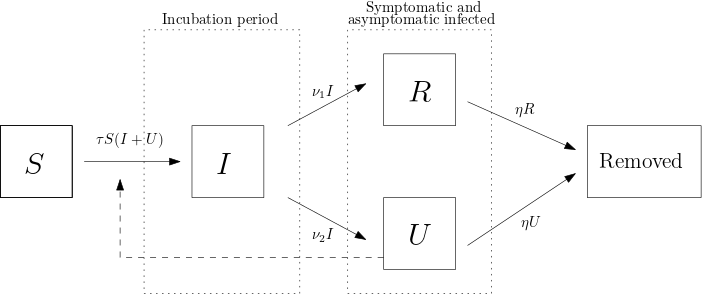
Figure 1: Diagram flux

The differential equations attached to the diagram above and that govern the dynamics of the epidemic are the following:

$$\left\{\begin{array}[]{l}S^{\prime}(t)=-\tau S(t)[I(t)+U(t)]\\ I^{\prime}(t)=\tau S(t)[I(t)+U(t)]-\nu I(t)\\ R^{\prime}(t)=\nu_{1}I(t)-\eta R(t)\\ U^{\prime}(t)=\nu_{2}I(t)-\eta U(t),\end{array}\right.$$ (1)

where $t\geq t_{0}$ corresponds to time, with $t_{0}$ being the starting date for the study (as in [10, 11, 12], in the implementation, we will consider the time $t_{0}$ corresponding to the beginning of the epidemic). Although this system of differential equations makes perfect sense when prescribing any initial condition, in epidemiological modeling one is naturally lead to use data of the following type:

$$S(t_{0})=S_{0}>0,\quad I(t_{0})=I_{0}>0,\quad R(t_{0})\geq 0\quad\mbox{and}\quad U(t_{0})=U_{0}\geq 0.$$

The parameters used in the model are described in the Table below. In particular, note that $\nu=\nu_{1}+\nu_{2}$. In addition, all the parameters that are considered $\tau,\nu,\nu_{1},\nu_{2},\eta$ are positive.

Symbol	Interpretation
$t_{0}$	Initial time.
$S_{0}$	Number of individuals susceptible to the disease at time $t_{0}$.
$I_{0}$	Number of infected individuals (in incubation period) without symptoms at time $t_{0}$.
$R_{0}$	Number of reported infected individuals at time $t_{0}$.
$U_{0}$	Number of unreported infected individuals at time $t_{0}$.
$\tau$	Transmission rate of the disease.
$1/\nu$	Average time during which the infectious asymptomatic individuals remain in incubation.
$f$	Fraction of asymptomatic infected individuals that become reported infected.
$\nu_{1}=f\nu$	Rate at which asymptomatic infected cases become reported.
$\nu_{2}=(1-f)\nu$	Rate at which asymptomatic infected become unreported infected individuals (asymptomatic or mildly symptomatic).
$1/\eta$	Average time during which an infected individual presents symptoms.

Table 1: Parameters and initial conditions of the model.

Note that in the first of the equations of (1), namely

$$S^{\prime}(t)=-\tau S(t)\,[I(t)+U(t)],$$

the role of $I$ and $U$ in the spread of the infection is the same. This is the essential point of the model: it gives the same dynamic role to those who are infected and do not have symptoms as to those who are not reported, because the latter do not go into quarantine and, in fact, have a similar social activity. Certainly, the model can be refined in many directions; for example, one could give different though still dynamical roles to $I$ and $U$ by attaching to them different positive parameters $\tau_{1}\neq\tau_{2}$ (this could be justified by that $U$ includes individuals with low symptomaticity who can practice self-care). However, it is already worth to visualize some of the main properties of this model and to implement it in specific situations following this general format.

2.2 Some basic qualitative properties

We next consider the system of equations (1) in more detail. We will assume an epidemic situation, which is summarized by the condition

$$\tau S_{0}-\nu>0.$$ (2)

We will also consider the initial conditions of Liu, Magal, Seydi and Webb:

$$S_{0}>0,\,\,I_{0}>0,\,\,R_{0}=0\,\,\mbox{ and }\,\,U_{0}=\frac{\nu_{2}\,I_{0}}{\eta+\chi_{2}}$$ (3)

for a certain $\chi_{2}>0$. (The precise value of the parameter $\chi_{2}$ will be given in the next section; here we just retain the fact that it is positive.) For simplicity, our starting time will be $t_{0}:=0$.

Theorem 2.1.

In an epidemic situation (2) and starting with the initial conditions (3), the following three properties are fulfilled:

1. For all time $t>0$, the values of $S(t)$, $U(t),I(t)$ and $R(t)$ exist, are positive and strictly smaller than $P:=S_{0}+I_{0}+U_{0}$ (the total population);

2. $S(t)$ converges to a certain positive limit value $S_{\infty}$ as $t\to\infty$, while $I(t),R(t),U(t)$ converge to $0$;

3. $R(t)/U(t)$ converges to $\nu_{1}/\nu_{2}$ from below.

Proof.

We first note that, due to (2) and (3), we have

$$S^{\prime}(0)=-\tau S_{0}I_{0}<0,$$

$$I^{\prime}(0)=(\tau S_{0}-\nu)I_{0}+\tau S_{0}U_{0}>0,$$

$$R^{\prime}(0)=\nu_{1}I_{0}>0,$$

$$U^{\prime}(0)=\nu_{2}I_{0}-\eta U_{0}=\nu_{2}I_{0}\left(1-\frac{\eta}{\eta+\chi_{2}}\right)>0.$$

Therefore, there exists $\varepsilon>0$ such that $S(t),I(t),R(t)$ and $U(t)$ (are defined in $[0,\varepsilon)$ and) are strictly positive. The arguments that follow are inspired by an observation contained in the classical book of Vladimir Arnold [1].

(i) Suppose $S$ vanishes, and let $T>0$ be the first time this occurs. Let $C>0$ be such that $I(t)+U(t)\leq C$ for all $t\in[0,T]$. Then $S^{\prime}(t)\geq-\tau CS(t)$, and hence, for $t\in[0,T)$, we have

$$\frac{S^{\prime}(t)}{S(t)}\geq-\tau C.$$

Integrating between $0$ and $s<T$, this gives

$$\log(S(s))-\log(S_{0})\geq-\tau Cs,$$

and then,

$$S(s)\geq S_{0}\,e^{-\tau Cs}.$$

Letting $s$ go to $T$, this contradicts the assumption $S(T)=0$.

Suppose now that $U$ vanishes, and let $T>0$ be the first time this occurs. If $I$ has not vanished until this time, then $U^{\prime}(t)=\nu_{2}I(t)-\eta U(t)\geq-\eta U(t)$ for all $t\in[0,T]$. By integration, this gives

$$U(T)\geq U_{0}\,e^{-\eta T},$$

which contradicts our assumption. Hence, $I$ should have vanished in $[0,T]$.

The same argument above shows that if $R$ vanishes at a time $T>0$, then $I$ must have vanished at some time in $[0,T]$.

Finally, suppose that $I$ vanishes, and let $T$ be the first moment this occurs. Then, $U(t)\geq 0$ for all $t\in[0,T]$, and therefore

$$I^{\prime}(t)=\tau S(t)\,[I(t)+U(t)]-\nu I(t)\geq-\nu I(t).$$

However, by integration, this again gives a contradiction, namely $I(T)\geq I_{0}e^{-\nu T}$.

We next show that neither $I$ nor $U$ explode (that is, none of them tends to infinity along an increasing sequence of times tending to a finite time $T$). Indeed, if anyone does it in time $T$ then, from the above, $P\geq S(t)\geq 0$ on $[0,T)$, and $U,I$ are positive on this interval. Therefore, on $[0,T)$,

$$(I+U)^{\prime}=\tau P\,[I+U]-\nu_{1}I-\eta U\leq\tau P\,[I+U],$$

which implies by integration that $(I+U)(t)\leq(I_{0}+U_{0})\,e^{\tau Pt}$ for $t\in[0,T)$. Letting $t$ go to $T$, this contradicts the explosion.

To see that $R$ does not explode, we proceed again by contradiction: if this occurs at time $T$, then from $R=\nu_{1}I-\eta R\leq\nu_{1}I$ we deduce $R(t)\leq R_{0}\,e^{\nu_{1}C}$ for all $t\in[0,T)$ and $C:=\max_{t\in[0,T]}I(t)$.

Finally, $S$ does not explode because it is decreasing and positive.

In conclusion, $S,I,R,U$ are all positive and do not explode. To prove that they are bounded from above by $P$, we introduce the equation of the deletted (removed) individuals from the system:

$$D^{\prime}(t)=\eta\,[R(t)+U(t)],\qquad D(0)=0.$$

We have a constant population $P=S(t)+I(t)+R(t)+U(t)+D(t)$, and since $D^{\prime}>0$, we have that $D(t)>0$ for all $t>0$. Now, since $S,I,R,U$ are positive for $t>0$, we conclude that each of them must be strictly smaller than $P$.

(ii) First we show that $S$ converges towards a positive limit. Let $S_{\infty}$ be the limit of $S$ (which exists because $S$ is decreasing). Denoting $c:=\min\{\eta,\nu\}$, we have

$$(I+U)^{\prime}=\tau S\,[I+U]-\nu_{1}I-\eta U\leq(\tau S-c)\,(I+U).$$

Since $S^{\prime}=-\tau S\,[I+U]$, this implies

$$(I+U)^{\prime}\leq\frac{(\tau S-c)\,S^{\prime}}{-\tau S}=-S^{\prime}+\frac{c}{\tau}\frac{S^{\prime}}{S}.$$

Integrating between $0$ and $t>0$, this gives

$$(I+U+S)(t)-(I_{0}+U_{0}+S_{0})\leq\frac{c}{\tau}\log\left(\frac{S(t)}{S_{0}}\right).$$

Since $I_{0}+U_{0}+S_{0}=P$, this implies

$$-P\leq\frac{c}{\tau}\log\left(\frac{S(t)}{S_{0}}\right).$$

Thus, for all $t>0$, we have   $S(t)\geq S_{0}e^{-\frac{\tau}{c}P},$   and therefore,   $S_{\infty}\geq S_{0}e^{-\frac{\tau}{c}P}>0.$

Next, we simultaneously prove that $I$ and $U$ converge to $0$ (the convergence of $R$ to $0$ will be then a consequence of the convergence of $R/U$ to $\nu_{1}/\nu_{2}$ proved in (iii) below). To do this, we first note that, since

$$S^{\prime}=-\tau S\,[I+U],$$

it follows that there is a sequence of times $t_{n}\to\infty$ such that $(I+U)(t_{n})\to 0$. Otherwise, there would exist $c>0$ such that $(I+U)(t)\geq c$ for all $t>0$, which implies $S^{\prime}/S\leq-\tau c$, and therefore $S(t)\leq S_{0}e^{-c\tau t}$. However, for $t$ large enough, this contradicts the inequality $S(t)\geq S_{\infty}>0$.

Now, since $\varepsilon>0$, we may fix $T$ such that $(I+U)(T)\leq\varepsilon/2$ and $S(t)\leq S_{\infty}+\varepsilon/2$ for all $t\geq T$. We claim that $(I+U)(t)\leq\varepsilon$ for all $t\geq T$. (Since $\varepsilon>0$ was arbitrarily chosen, this concludes the proof of the convergence of $I+U$ towards $0$.) To prove this, note that, since $(S+I+U)^{\prime}(t)=-\nu_{1}I-\eta U<0$, we have $(S+I+U)(t)\leq(S+I+U)(T)$ for all $t\geq T$, hence

$$(I+U)(t)\leq(I+U)(T)+[S(T)-S(t)]\leq\frac{\varepsilon}{2}+\frac{\varepsilon}{2}=\varepsilon,$$

as we wanted to show.

(iii) To prove that $R/U$ converges to $\nu_{1}/\nu_{2}$, we first remark that

$$\left(\frac{R}{U}\right)^{\prime}=\frac{R^{\prime}U-RU^{\prime}}{U^{2}}=\frac{(\nu_{1}I-\eta R)\,U-R\,(\nu_{2}I-\eta U)}{U^{2}}=\nu_{2}\,\frac{I}{U}\left(\frac{\nu_{1}}{\nu_{2}}-\frac{R}{U}\right).$$ (4)

Therefore,

$$\frac{R}{U}>\frac{\nu_{1}}{\nu_{2}}\Longrightarrow\left(\frac{R}{U}\right)^{\prime}(t)<0,$$

$$\frac{R}{U}<\frac{\nu_{1}}{\nu_{2}}\Longrightarrow\left(\frac{R}{U}\right)^{\prime}(t)>0.$$

In other words, if $R/U$ is smaller (resp. greater) than $\nu_{1}/\nu_{2}$ at a point $t$, then it is increasing (resp. decreasing) around this point.

We first prove that $R/U$ cannot be equal to $\nu_{1}/\nu_{2}$ at any point. To do this, we note that $R_{0}/U_{0}=0\neq\nu_{1}/\nu_{2}$. We define $\varphi:=\frac{\nu_{1}}{\nu_{2}}-\frac{R}{U}$. Equality (4) then becomes

$$\varphi^{\prime}=-\nu_{2}\frac{I}{U}\varphi.$$

If $T$ were the first instant at which $R/U=\nu_{1}/\nu_{2}$, then $T$ would be the first zero of $\varphi$. By (i), there exists $C>0$ such that $\nu_{2}I/U\leq C$ on $[0,T]$. Since $R_{0}=0$, one has $\varphi(t)>0$ for all positive but small-enough $t$. Choosing such a $t$ smaller than $T$ we obtain, on $[t,T),$

$$\frac{\varphi^{\prime}}{\varphi}\geq-C.$$

By integration, this gives $\varphi(T)\geq\varphi(t)\,e^{t-T}$, which contradicts the fact that $\varphi(T)=0$.

To prove the convergence of $R/U$ towards $\nu_{1}/\nu_{2}$, which is equivalent to that of $\varphi$ towards $0$, we will use the fact (proven below) that $I/U$ is bounded from below by a positive constant $c$. Assuming this, we have

$$\frac{\varphi^{\prime}}{\varphi}\leq-\nu_{2}\,c,$$

and hence,

$$\varphi(T)\leq\varphi(t)\,e^{(t-T)\nu_{2}c},$$

which converges to $0$ as $T\to\infty$.

To conclude, we must show that $I/U$ does not approach zero. For this, we begin by noting that

$$\left(\frac{I}{U}\right)^{\prime}=\frac{I^{\prime}U-IU^{\prime}}{U^{2}}=\frac{(\tau S\,[I+U]-\nu I)\,U-I\,(\nu_{2}I-\eta U)}{U^{2}}=\tau S-\nu_{2}\left(\frac{I}{U}\right)^{2}+\frac{I}{U}(\tau S+\eta-\nu).$$

Since $S\geq S_{\infty}$, if $I/U$ is very small, then the derivative $(I/U)^{\prime}$ becomes positive, and therefore $I/U$ grows. As a consequence, $I/U$ cannot arbitrarily approximate $0$. ∎

There are several remarks to the proof above.

Remark 2.2.

The proof above applies to more general initial conditions than (3): it only requires that the values $S_{0}>0,I_{0}>0,R_{0}\geq 0$ and $U_{0}\geq 0$ are such that $I^{\prime}(t_{0})$, $R^{\prime}(t_{0})$ and $U^{\prime}(t_{0})$ are all positive. However, note that, at this level of generality, in statement (iii) above the convergence of $R/U$ towards $\nu_{1}/\nu_{2}$ can occur from above, and even the quotient $R/U$ can remain constant and equal to $\nu_{1}/\nu_{2}$ throughout the whole evolution.

Remark 2.3.

In the classical SIR model, the fact that the population of susceptibles converges towards a positive limit is often presented as a consequence of the so-called final size relation [5]. In our context, $S^{\prime}$ not only depends on $I$, but also on $U$. For this reason, it is hard to expect such a simple relation, and this partly justifies the use of robust estimates in the preceding proof.

Remark 2.4.

The convergence of $R$ and $U$ towards $0$ must hold at a speed lower than $e^{-\eta t}$. Indeed, from the last two equations of the system one obtains

$$\frac{R^{\prime}+\eta R}{\nu_{1}}=I=\frac{U^{\prime}+\eta U}{\nu_{2}},$$

which can be rewritten in the form $\nu_{2}(Re^{\eta t})^{\prime}=\nu_{1}(Ue^{\eta t})^{\prime}$. By integration, this gives

$$\nu_{2}Re^{\eta t}=\nu_{1}Ue^{\eta t}+C,\qquad\mbox{where}\quad C:=-\nu_{1}U_{0}.$$

Therefore,

$$\frac{R}{U}=\frac{\nu_{1}}{\nu_{2}}+\frac{C}{\nu_{2}\,Ue^{\eta t}}.$$

Since $R/U$ converges to $\nu_{1}/\nu_{2}$, the product $Ue^{\eta t}$ must tend to infinity, thus showing our claim for $U$. The claim for $R$ immediately follows from this.

Remark 2.5.

Another observation is related to the proportion $R/U$. Since this number grows throughout the epidemic, the dynamic variability that we mentioned at the beginning of this work holds. Moreover, the convergence of $R/U$ towards $\nu_{1}/\nu_{2}$ tells us what should be the values of the parameters in the implementation. We will return to this point for a specific case in the next section.

Remark 2.6.

Finally, we must mention that one of the basic results on the SIR model has not been incorporated into the theorem above, namely, that of the uniqueness of the peak of the curve of infected cases. In fact, this uniqueness is no longer valid for the SIRU model. Below we draw an example of a double peak for the reported and unreported cases curves. Note that though this occurs under initial conditions different from (3), it holds in a context in which the theorem is still valid, according to Remark 2.2.

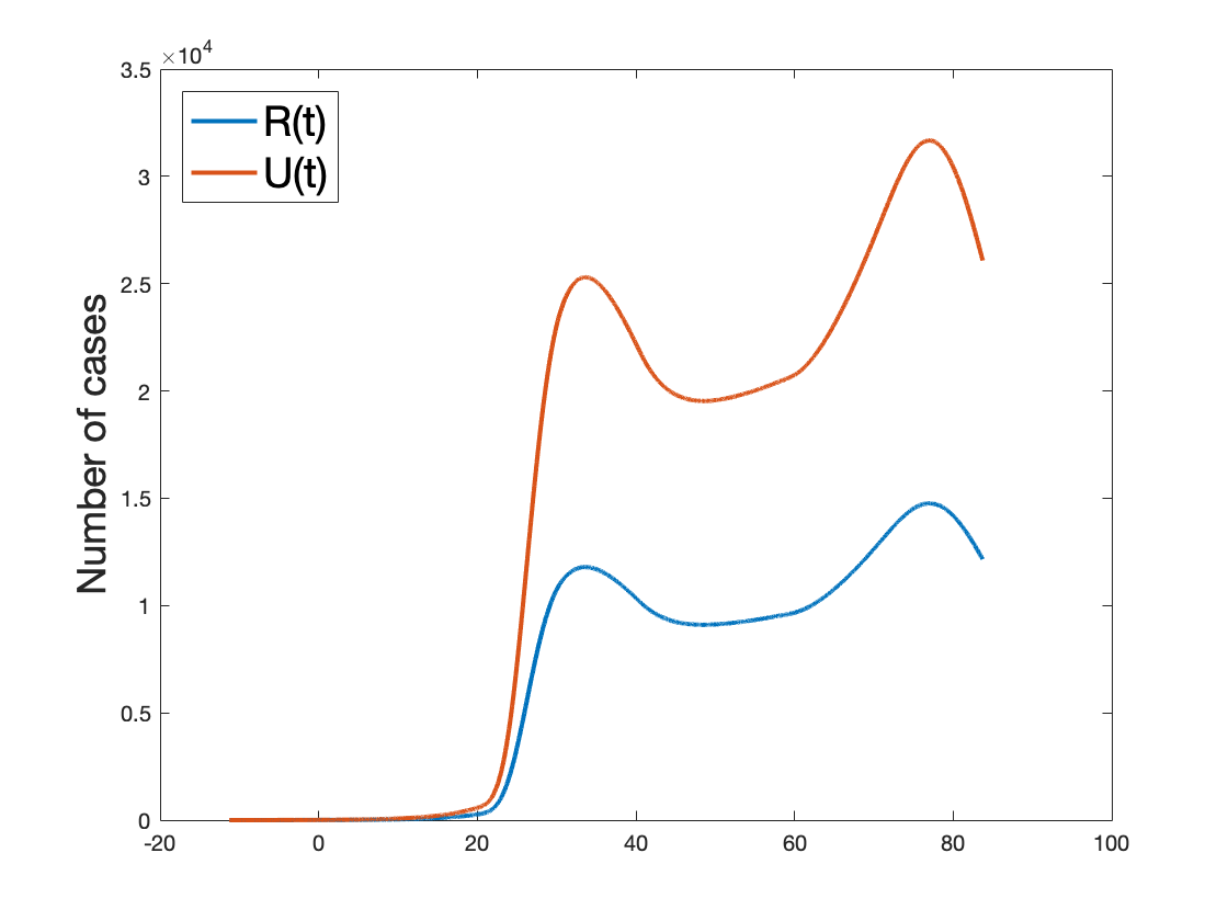
Figure 2: A double peak for the curves.

Examples of this type can be easily obtained. For the curve $R$, one starts by imposing the conditions $R^{\prime}(t_{p})=0$ and $R^{\prime\prime}(t_{p})>0$ for a time $t_{p}>0$ different from the starting time. These conditions can be translated into conditions only on the values of $S,I,R$ and $U$ at that time. Then the SIRU equations are implemented in both directions of time around $t_{p}$. This moment will hence correspond to a local minimum of the curve, necessarily located between two peaks.

The same argument allows to build examples in which the curve of infected cases has two peaks. Naturally, this is due to the presence of $U$ in the derivative of $I$, which is an absent element of the SIR model. In fact, in this one, the condition $I^{\prime}=0$ necessarily implies $I^{\prime\prime}<0$, as a straightforward computation shows. This occurs only at the peak of the curve, which corresponds to the time when herd immunity is achieved.

3 Observations based on official numbers

3.1 General implementation of the SIRU model

Our goal now is to compare the data available on COVID-19 in Chile until May 14 (2020) [13] with what is predicted by the SIRU model, so that we can estimate the evolution of the number of unreported cases throughout the period. We point out that a first estimate of unreported cases in (some regions of) Chile using the data of March 2020 and the SIRU model was carried out by Mónica Candia and Gastón Vergara-Hermosilla in [6].

To begin with, let us point out that in outbreaks of influenza disease, the parameters $\tau,\ \nu,\ \nu_{1},\ \nu_{2},\ \eta$, as well as the initial values $S_{0},I_{0}$ and $U_{0}$, are generally unknown. However, it is possible to identify them from specific time data of reported symptomatic cases. The cumulative number of infectious cases reported at a time $t$, denoted by $CR(t)$, is given by

$$CR(t):=\nu_{1}\int_{t_{0}}^{t}I(s)ds.$$

This is data that is openly available. Likewise, the cumulative number of unreported cases at a time $t$ is

$$CU(t):=\nu_{2}\int_{t_{0}}^{t}I(s)ds.$$

We note that, up to constants, these values coincide respectively with

$$R(t)+\eta\int_{t_{0}}^{t}R(s)\,ds\qquad\mbox{ and }\qquad U(t)+\eta\int_{t_{0}}^{t}U(s)\,ds.$$

Following the scheme used by Liu, Magal, Seydi and Webb, we will assume that, at an early stage of the disease, $CR(t)$ has an (almost) exponential form:

$$CR(t)=\chi_{1}\exp(\chi_{2}t)-\chi_{3}.$$

For simplicity, we will assume that $\chi_{3}=1$. The values of $\chi_{1}$ and $\chi_{2}$ will then be adjusted to the accumulated data of cases reported in the early phase of the epidemic using a classical least squares method (after passing to logarithmic coordinates). According to the above (see [10] for details), for numerical simulations, the initial time for the beginning of the exponential growth phase is fitted at

$$t_{0}:=-\frac{1}{\chi_{2}}\cdot\log\left(\chi_{1}\right).$$

Again, for simplicity, we will identify the initial value $S_{0}$ to that of the total population of Chile (since there is no prior immunity against the virus). Once the values of $\nu$, $\eta$ and $f$ are set, the conditions at the beginning of the disease are naturally fitted as

$$I_{0}:=\frac{\chi_{2}}{f\left(\nu_{1}+\nu_{2}\right)}=\frac{\chi_{2}}{\nu_{1}},\quad U_{0}:=\left(\frac{(1-f)\left(\nu_{1}+\nu_{2}\right)}{\eta+\chi_{2}}\right)I_{0}=\frac{\nu_{2}\,I_{0}}{\eta+\chi_{2}},\quad R_{0}:=0.$$

We recall that $1/\nu$ corresponds to the average time during which patients are asymptomatic infectious. As in [10, 11, 12], we will let this parameter be equal to 7 (days), and the same value will be used for the average time in which patients are reported or unreported infectious:

$$\tau=\eta=1/7.$$

Note that although the incubation period has been reported as being slightly smaller, the lag in the delivery of the results of the PCR tests in Chile justifies this choice.

3.2 On the fraction of unreported cases

To implement the SIRU system we still need to establish a good value for the parameter $f$ (the fraction of symptomatic cases that are reported). Once this is fitted, we will have the values of

$$\nu_{1}=f\nu\quad\mbox{ y }\quad\nu_{2}=(1-f)\nu,$$

and we will just need to fit the value of $\tau$.

Before continuing, it is worth pointing out that in [10, 11, 12] there is no major discussion on the criterion used to establish the value of $f$ in the different scenarios. Actually, a value issued by the medical counterpart is assumed as valid. (For example, $f=0.8$ is considered for China.) In our modeling, we will use the work of Baeza-Yates [4] and that of Castillo and Pastén [7], who use the case fatality rate of the disease (with the correct correction according to its duration; see [2, 9]) to give estimates for the right number of infected individuals. Since Baeza-Yates’ argument is simpler and is not included in an academic publication, we borrow it below in a language closer to that of the SIRU model. As we will see, it yields a method to adjusting the value of $f$ that can be used in almost all contexts.

Since we know that $R/U$ converges towards $\nu_{1}/\nu_{2}$, we assume for this calculation that $R/U$ is simply equal to $\nu_{1}/\nu_{2}$. In addition, we will argue in discrete units of time (in days). Then we have

$$R(n)=f\,[R(n)+U(n)]$$

If $d$ is the average time of illness to death and $M(n)$ the number of deaths in day $n$, then the case fatality rate $L$ corresponds to

$$L=\frac{M(n)}{[R(n-d)+U(n-d)]}.$$

Moreover, the reported case fatality rate is

$$L_{R}=\frac{M(n)}{R(n-d)}=\frac{M(n)}{[R(n-d)+U(n-d)]}\cdot\frac{[R(n-d)+U(n-d)]}{R(n-d)}=\frac{L}{f}.$$

This gives

$$f=\frac{L}{L_{R}}.$$

In the Chilean context, deaths in the period studied occurred within $9.4$ days after the disease was reported. Adjusting $d=9$, the computation of $L_{R}$ is made feasible from the data available in [13].

Finally, regarding the natural case fatality ratio $L$ of the disease, it is deduced from international studies that, after adjusting it to the age distribution of the Chilean population, it should vary between $0.2\%$ and $1\%$, with a very high tendency to be around $0.6\%$. In summary, this gives a parameter $f$ varying between $0.1$ and $0.5$, with a high tendency to be close to $\frac{1}{3.4}\sim 0.3$.

3.3 Variations in the transmission rate

Given the heterogeneity of the safeguard measures taken by the Chilean government, instead of directly applying the SIRU model, it became more pertinent to us to consider a variable transmission rate $\tau$ (as a function of time). To analyze the variation of the values of $\tau(t)$, we observe how the percentage of the Chilean population subjected to confinement has been changing, which is illustrated below:

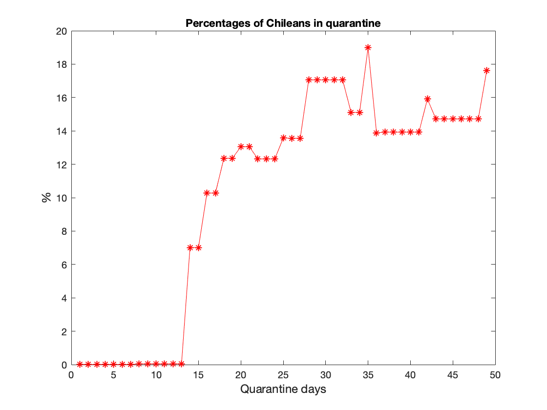
Figure 3: Variation of the percentages of the population in quarantine in Chile corresponding to the first 49 days from March 13, 2020.

We hence propose a function $\tau(t)$ of the form

$$\tau(t)=\left\{\begin{array}[]{ll}\tau_{0}&\mbox{ if }t\in\mathcal{I}_{1}=[N_{0},N_{1}],\\ \tau_{1}(t)=\tau_{0}\exp(-\mu_{1}(t-N_{1}))&\mbox{ if }t\in\mathcal{I}_{2}=(N_{1},N_{2}],\\ \vdots&\,\,\vdots\\ \tau_{r}(t)=\tau_{r-1}(t)\exp(-\mu_{r-1}(t-N_{r-1}))&\mbox{ if }t\in\mathcal{I}_{r}=(N_{r-1},N_{r}],\end{array}\right.$$

where the $\mathcal{I}_{i}$’s correspond to successive time intervals. For the Chilean context, according to the graph of quarantines illustrated above (Figure 3), the chosen time intervals are those described in Table 2 below:

Interval	Time frame	$N_{i}$
$\mathcal{I}_{1}$	from March 3 to 22	March 22
$\mathcal{I}_{2}$	from March 23 to April 1	April 1
$\mathcal{I}_{3}$	from April 2 to 11	April 11
$\mathcal{I}_{4}$	from April 12 to 21	April 21
$\mathcal{I}_{5}$	from April 22 to 31	April 31
$\mathcal{I}_{6}$	from May 1 to 10	May 10
$\mathcal{I}_{7}$	from May 11 to 14	May 14

Table 2: Time intervals used in our numerical simulations.

Following [10, 11, 12], the value of the transmission rate in $\mathcal{I}_{1}$ is fitted to

$$\tau_{0}:=\left(\frac{\chi_{2}+\nu}{S_{0}}\right)\left(\frac{\eta+\chi_{2}}{\nu_{2}+\eta+\chi_{2}}\right).$$

Then, the parameters $\mu_{i}$ are chosen in such a way that the reported cumulated cases in the numerical simulation align with the data of the reported cumulative number of infections at time $t$ according to [13]. This is implemented with various values of $f$, following the guidelines of the preceding subsection (specifically, we work with $f=0.2$, $f=0.3$ and $f=0.4$). A summary is described in the following Table:

Parameter	$f=0.2$	$f=0.3$	$f=0.4$
$\mu_{1}$	8.3$\cdot 10^{-4}$	8.3$\cdot 10^{-4}$	8.3$\cdot 10^{-4}$
$\mu_{2}$	2.1$\cdot 10^{-6}$	2.1$\cdot 10^{-6}$	2.1$\cdot 10^{-6}$
$\mu_{3}$	5$\cdot 10^{-6}$	5$\cdot 10^{-6}$	5$\cdot 10^{-6}$
$\mu_{4}$	1.41$\cdot 10^{-6}$	1.41$\cdot 10^{-6}$	1.41$\cdot 10^{-6}$
$\mu_{5}$	5.08$\cdot 10^{-5}$	5.08$\cdot 10^{-5}$	5.08$\cdot 10^{-5}$
$\mu_{6}$	2.96$\cdot 10^{-4}$	2.96$\cdot 10^{-4}$	2.96$\cdot 10^{-4}$

Table 3: Parameters $\mu_{i}$ corresponding to the different values of $f$ considered in our numerical simulations.

Using the data of the cumulated reported cases available in [13], we can finally proceed to the simulations, which are shown below. They illustrate numerical estimates for the curves of $CR(t),\ CU(t),\ R(t)$ and $U(t)$.

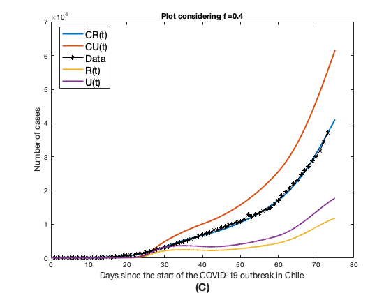
Figure 4: Plots of the numerical approximations of the functions $CR(t),\ CU(t),\ R(t)$ and $U(t)$ obtained from the numerical solutions of the model (1) applied to the Chilean context based on the data of reported cumulated cases up to 14 May 2020 [13]. The plots (A), (B) and (C) were obtained by considering $f=0.2$, $f=0.3$ and $f=0.4$ respectively, using the parameters $\eta=1/7$ and $\nu=1/7$.

Discussion and future work

The epidemic outbreak of the new human coronavirus COVID-19 was first detected in Wuhan, China, in late 2019. In Chile, the first case was reported on March 3, 2020, in Talca (Maule region). Since then, modeling the epidemic in the country has faced the problem of the low availability of disaggregated data [3].

The first part of this work was inspired by the situation experienced in Chile during the month of April, when the number of reported cases stabilized around 450 per day. According to most specialists, this was not accurately representing the genuine epidemiological evolution. Although it is difficult to argue that our reasoning from the first section fully applies to this situation (in particular, because the number of daily tests during the period was variable), the explosive increase of cases that subsequently occurred should call us to reflection on the point. Nevetheless, it is clear that this increase was also due in part to the relaxation of the protection measures, which is reflected not only in the absolute (and exponential) increase in the number of cases, but also in the proportion of positive cases with respect to tests (the latter despite of the significant increase in the number of tests [8]).

The first part of the work naturally led us to model the dynamics of the epidemic incorporating a compartment for unreported cases so that we could deal with their active role in the evolution. To do this, we used the SIRU model recently introduced/implemented by Liu, Magal, Seydi and Webb in [10, 11, 12]. Since the qualitative theory of the underlying differential equations has not yet been treated, we developed some essenttial points of it in the second section, thus rigorously establishing fundamental structure theorems. However, we pointed out an important difference with the SIR model, namely, the possibility of multiple peaks for the curves of infected, reported and unreported patients. For the future, it would be desirable to complete the qualitative description of the solutions of the equations with respect to the parameters, with an emphasis on the phenomenon of multiplicity of peaks. For example, until now we do not know whether there can be more than two peaks and/or whether there is any restriction on the relative position between them. Without any doubt, this discussion is relevant for the implementation of disease containment policies, since it is directly related to the recognition of the moment when the curves begin to definitively descend.

In the last section of the work, we implemented an extension of the model to the case of Chile. To do this, we considered a variable transmission rate, which is more appropriate according to the local reality. Our rate is coupled to the official statistics provided by the government in [13], information that also allowed us to make the parametric afjustement. The last ingredient to launch the simulations was to fit the value of the fraction $f$ of infected individuals that were reported during the period of study. For this we used the work of Baeza-Yates [4] and that of Castillo and Pastén [7]. Naturally, our modeling is consistent with their estimates. In particular, in Section 2.3 of [7], the authors estimate the number of real cases for April 28 as 43095, which is remarkably close to the number of total cases that can be inferred from the plot (B) in Figure 4 obtained by considering $f=0.3$. We point out that the prediction of Castillo and Pastén is recovered with complete accuracy through the method used in this work for the value $f=0.31791$. According to our modeling, on April 28, a percentage of $31.791\%$ of the infections was reported to health agencies, and consequently $68.209\%$ of the infected cases was not reported.

Although the estimates above were obtained a posteriori, their complementarity puts us in a good position to use them for modeling the future evolution of the epidemic. However, working in this direction requires great caution. In particular, it would be necessary to consider a variable parameter $f$, since both the quantity and the criteria of the tests have been modified during late May. Despite this, we strongly believe that the basis for pursuing the implementation of the SIRU model are fullfilled, and it would be very useful to advance in a more compartmentalized and georeferenced implementation of it.

Acknowledgments. We would like to thank María Paz Bertoglia, Mónica Candia, Alicia Dickenstein, Yamileth Granizo, Rafael Labarca, Mario Ponce and Marius Tucsnak for their reading, their kind remarks and suggestions of bibliography.

Andrés Navas

Dpto. de Matemáticas y Ciencias de la Computación,

Universidad de Santiago de Chile

e-mail: andres.navas@usach.cl

Gastón Vergara-Hermosilla

Institut de Mathématiques de Bordeaux,

Université de Bordeaux, Francia

e-mail: gaston.vergara@u-bordeaux.fr

References

- [1] Vladimir Arnold. Ordinary Differential Equations. Nauka, Moscow (1971).
- [2] Avner Ban-Hen. Taux de mortalité du virus Ébola. Images des Mathématiques. https://images.math.cnrs.fr/Taux-de-mortalite-du-virus-Ebola.html
- [3] Ricardo Baeza-Yates. Datos de calidad y el coronavirus. Medium, https://medium.com/@rbaeza-yates/datos-de-calidad-y-el-corona-virus-98893b7600e3
- [4] Ricardo Baeza-Yates. https://twitter.com/PolarBearby/status/1256673286022295553
- [5] Fred Brauer & Carlos Castillo-Chavez. Mathematical Models in Population Biology and Epidemiology. Texts in Applied Mathematics, Springer Verlag (2001).
- [6] Mónica Candia & Gastón Vergara-Hermosilla. Estimación de casos no reportados de infectados de COVID-19 en Chile, el Maule y la Araucanía durante marzo de 2020. Preprint (April 2020), available at https://hal.archives-ouvertes.fr/hal-02560526/
- [7] Jorge Castillo Sepúlveda & Héctor Pastén. Información escondida en los datos inciertos sobre el COVID-19 en Chile. Preprint (April 2020), available at http://www.mat.uc.cl/hector.pasten/preprints/InfoEscondida.pdf
- [8] Felipe Elorrieta, Claudio Vargas, Fernando A. Crespo, Valentina Navarro, Francisco Oviedo y Camila Guerrero. Dudas sobre el incremento de contagios por coronavirus: ¿hay un rebrote o sólo se debe a que estamos haciendo más test? CIPER Académico, https://ciperchile.cl/2020/05/06/dudas-sobre-el-incremento-de-contagios-por-coronavirus-hay-un-rebrote-o-solo-se-debe-a-que-estamos-haciendo-mas-test/
- [9] A. C. Ghani, C. A. Donnelly, D. R. Cox, J. T. Griffin, C. Fraser, T. H. Lam, L. M. Ho, W. S. Chan, R. M. Anderson, A. J. Hedley & G. M. Leung. Methods for estimating the case fatality ratio for a novel, emerging infectious disease. American Journal of Epidemiology 162 (5) (2005), 479-486.
- [10] Zhihua Liu, Pierre Magal, Ousmane Seydi & Glenn Webb. Understanding unreported cases in the COVID-19 epidemic outbreak in Wuhan, China, and the importance of major public health interventions. Biology, vol. 9 (3) (2020).
- [11] Zhihua Liu, Pierre Magal & Glenn Webb. Predicting the number of reported and unreported cases for the COVID-19 epidemics in China, South Korea, Italy, France, Germany and United Kingdom. Preprint (April 2020).
- [12] Zhihua Liu, Pierre Magal, Ousmane Seydi & Glenn Webb. A model to predict COVID-19 epidemics with applications to South Korea, Italy, and Spain, SIAM News (to appear).
- [13] Official data on COVID-19 from the Chilean government (in Spanish). https://www.gob.cl/coronavirus/cifrasoficiales