Double Generative Adversarial Networks for Conditional Independence Testing
Abstract
In this article, we study the problem of high-dimensional conditional independence testing, a key building block in statistics and machine learning. We propose an inferential procedure based on double generative adversarial networks (GANs). Specifically, we first introduce a double GANs framework to learn two generators of the conditional distributions. We then integrate the two generators to construct a test statistic, which takes the form of the maximum of generalized covariance measures of multiple transformation functions. We also employ data-splitting and cross-fitting to minimize the conditions on the generators to achieve the desired asymptotic properties, and employ multiplier bootstrap to obtain the corresponding -value. We show that the constructed test statistic is doubly robust, and the resulting test both controls type-I error and has the power approaching one asymptotically. Also notably, we establish those theoretical guarantees under much weaker and practically more feasible conditions compared to the existing tests, and our proposal gives a concrete example of how to utilize some state-of-the-art deep learning tools, such as GANs, to help address a classical but challenging statistical problem. We demonstrate the efficacy of our test through both simulations and an application to an anti-cancer drug dataset. A Python implementation of the proposed procedure is available at https://github.com/tianlinxu312/dgcit.
Keywords: Conditional independence; Double-robustness; Generalized covariance measure; Generative adversarial networks; Multiplier bootstrap.
1 Introduction
Conditional independence (CI) is a fundamental concept in statistics and machine learning. Testing conditional independence is a key building block and plays a central role in a large variety of statistical learning problems, for instance, causal inference (Pearl, 2009), graphical models (Koller and Friedman, 2009), dimension reduction (Li, 2018), among many others. It is frequently used in a wide range of scientific and business applications, and we demonstrate its application with a cancer genetics example later.
In this article, we aim at testing whether two random variables and are conditionally independent given a set of confounding variables . That is, we test the hypotheses:
| (1) |
given the observed data of i.i.d. copies of . For our problem, and can all be multivariate. However, the main challenge arises when the confounding set of variables is multivariate and high-dimensional. As such, we primarily focus on the scenario where and are univariate, and is multivariate and its dimension can potentially diverge to infinity. Meanwhile, our proposed method can be readily extended to the scenario of multivariate and as well. Another challenge is the limited sample size compared to the dimensionality of . As a result, many existing tests may become ineffective, suffering from either an inflated type-I error, or not having enough power to detect the alternatives. See Section 2 for a detailed literature review.
To deal with those challenges, we propose a testing procedure based on double generative adversarial networks (GANs, Goodfellow et al., 2014) for the CI testing problem in (1). GANs have recently stood out as a powerful approach for learning and generating random samples from a complex, high-dimensional data distribution. They have been successfully applied in numerous applications, ranging from image processing and computer vision, to sequential data modeling such as natural language, music, speech, and to medical fields such as DNA design and drug discovery; see Gui et al. (2020) for a review of the GANs applications. Moreover, there have recently emerged works studying the consistency and rate of convergence of the GANs estimators; see, e.g., Liang (2018); Chen et al. (2020).
Our proposal involves two key components: a double GANs framework to learn two generators that approximate the conditional distribution of given , and given , respectively, and a test statistic that is taken as the maximum of generalized covariance measures of multiple transformation functions of and . We first show that our test statistic is doubly-robust, which offers an additional layer of protection against potential misspecification of the conditional distributions; see Theorems 2 and 3. We then show that the resulting test achieves a valid control of the type-I error asymptotically, and more importantly, under the set of conditions that are much weaker and practically more feasible compare to the existing tests; see Theorem 4. Besides, we prove that the power of our test approaches one asymptotically; see Theorem 5, and we demonstrate through simulations that it is more powerful than numerous competing tests empirically. In addition, we employ data splitting and cross-fitting that allow us to derive the asymptotic properties under minimal conditions on the generators, and employ multiplier bootstrap to obtain the corresponding -value of the test. Our contributions are multi-fold. We develop a useful testing procedure for a fundamentally important statistical inference problem. We establish the statistical guarantees under much weaker conditions. We also give an example of how to utilize some state-of-the-art deep learning tools, such as GANs, to address a classical but challenging statistical problem.
The rest of the article is organized as follows. Section 2 reviews some key existing CI testing methods. Section 3 develops the double GANs-based testing procedure. Section 4 derives the theoretical properties. Section 5 presents the simulations and a cancer genetics data example. Section 6 concludes the paper. The Appendix collects all technical proofs.
2 Literature review on conditional independence testing
There has been a large and growing literature on conditional independence testing; see Li and Fan (2019) for a review. Broadly speaking, the existing tests can be cast into four main categories, the metric-based tests (e.g., Su and White, 2007, 2014; Wang et al., 2015; Pan et al., 2017; Wang et al., 2018), the conditional randomization-based tests (e.g., Candes et al., 2018; Bellot and van der Schaar, 2019), the kernel-based tests (e.g., Fukumizu et al., 2008; Zhang et al., 2011), and the regression-based tests (e.g., Hoyer et al., 2009; Shah and Peters, 2018). There are also some other types of tests (e.g., Bergsma, 2004; Berrett et al., 2019, to name a few).
The metric-based tests typically employ some kernel smoothers to estimate the conditional characteristic function or the distribution function of given and . Kernel smoothers, however, are known to suffer from the curse of dimensionality, and as such, these tests are usually not suitable when the dimension of is high. The conditional randomization-based tests require the knowledge of the conditional distribution of (Candes et al., 2018). If unknown, the type-I error rates of these tests rely critically on the quality of the approximation of this conditional distribution. Kernel-based tests are built upon the notion of maximum mean discrepancy (MMD, Gretton et al., 2012), and could have inflated type-I errors. Regression-based tests have valid type-I error control, but may suffer from inadequate power.
Next, we discuss in detail the conditional randomization-based tests, in particular, the work of Bellot and van der Schaar (2019), the regression-based tests, and the MMD-based tests, as our proposal is related to and built on those methods. For each family of tests, we first lay out the main ideas, then discuss their potential limitations.
2.1 Conditional randomization-based tests
The family of conditional randomization-based tests is built upon the following basis. If the conditional distribution of given is known, then one can independently draw , for , where the superscript denotes the first round of draws. Besides, these samples are independent of the observed samples ’s and ’s. Write , , , and . Hereinafter we use boldface letters to denote data matrices that consist of samples. Since the joint distributions of and are the same under , any large difference between the two distributions can be interpreted as evidence against . Therefore, one can repeat the sample drawing process times, i.e., , , . Write . Then, for a given test statistic , the associated -value is
where denotes the indicator function. Since the triplets are exchangeable under , the above -value is valid, in the sense that it equals the significance level under the null, i.e.,
In practice, however, is rarely known. Bellot and van der Schaar (2019) proposed to approximate using GANs. Specifically, they learned a generator from the observed data, then took along with an independent noise variable as the input to obtain a sample , which minimizes the divergence between the distributions of and . They computed the -value by replacing with . They called this test the generative conditional independence test (GCIT). By Theorem 1 of Bellot and van der Schaar (2019), the excess type-I error of this test is upper bounded as,
| (2) |
where is the total variation norm between two probability distributions and such that , the supremum is taken over all measurable sets , and the expectations in (2) are taken with respect to .
By definition, the error term in (2) measures the quality of the conditional distribution approximation. Bellot and van der Schaar (2019) argued that this error term is negligible due to the capacity of deep neural networks in terms of estimating the conditional distribution. To the contrary, we find this approximation error is usually not negligible, and consequently, it may inflate the type-I error and invalidate the test. We consider a simple example to further elaborate this.
Example 1
Suppose is one-dimensional, and follows a simple linear regression model, , where the error is independent of , and for some .
Suppose we know a priori that the linear regression model holds. We thus estimate by ordinary least squares, and denote the resulting estimator by . For simplicity, suppose is known too. For this simple example, we have the following result regarding the approximation error .
Proposition 1
Suppose the linear regression model holds, the dimension of is much smaller than the sample size , and the derived distribution is , where is the identity matrix. Then does not decay to zero.
To facilitate the understanding of the convergence behavior of , we sketch a few lines of the proof of Proposition 1. The complete proof is given in the Appendix. Let denote the conditional distribution of given , which is in this example. If , then,
| (3) |
In other words, in order to control the type-I error, GCIT requires the total variation distance measure in (3) to converge at a faster rate than . However, this rate cannot be achieved in general. In our Example 1, we have for some constant . Consequently, in (2) is not . Proposition 1 shows that, even if we know a priori that the linear model holds, does not decay to zero as tends to infinity. In practice, we do not have such prior model information. Then it would be even more difficult to estimate the conditional distribution . Therefore, using GANs to approximate does not guarantee a negligible approximation error.
2.2 Regression-based tests
The family of regression-based tests is built upon the generalized covariance measure,
where and are the estimated condition means and , respectively, obtained by some supervised learner. When the prediction errors of and satisfy certain convergence rates, Shah and Peters (2018) proved that GCM is asymptotically normal under , in which the asymptotic mean is zero, and the standard deviation can be consistently estimated by some standard error estimator, denoted by . Therefore, at level , we reject , if exceeds the upper th quantile of a standard normal distribution.
Such a test can control the type-I error. Nevertheless, it may not have sufficient power to detect . Consider the asymptotic mean of GCM, which is . The regression-based tests require to be nonzero under to have power. However, it may be difficult to satisfy such a requirement. We again consider a simple example.
Example 2
Suppose , and are independent random variables. Besides, has mean zero, and for some function .
For this example, we have , since both and are independent of , and so is . Besides, , since is independent of and . Thus for any function . On the other hand, and are conditionally dependent given , as long as is not a constant function. Therefore, for this example, the regression-based tests would fail to discriminate between and .
2.3 MMD-based tests
The family of MMD-based tests involves the maximum mean discrepancy as a measure of independence. For any two probability measures , and a function space , define
Let , denote some function spaces of and . Define
where is the tensor product, is the joint distribution of whose definition does not rely on , and is the conditionally independent distribution with the same and margins as . Let and be independent copies of and , such that they are conditionally independent given . Then corresponds to the joint distribution of . Note that, to generate , we need to first sample according to , then generate and that follow and , respectively. As such, depends on , and depends on through . Furthermore, since , we have,
As such, measures the average conditional association between and given . Under , it equals zero, and hence an estimator of this measure can be used as a test statistic for . Moreover, if and are reproducing kernel Hilbert spaces (RKHSs), then has a closed form expression in terms of the reproducing kernels of the RKHS (Doran et al., 2014; Gretton et al., 2012), which makes the tests based on an estimator of easier to evaluate.
A notable example of this family is the kernel MMD-based test (KCIT) of Zhang et al. (2011). We next further discuss this test. To control the type-I error asymptotically, KCIT requires the dimension of to be fixed (Zhang et al., 2011, Proposition 5), since it uses the continuous mapping theorem to derive the limiting distribution of its test statistic. However, the continuous mapping theorem may not hold when diverges with . In addition, KCIT requires the distance between the covariance operator and its empirical estimator to decay to zero. It remains unknown whether such an assertion holds as diverges. By contrast, the test we develop allows to diverge while maintaining the asymptotic control of the type-I error. This implies that our test is expected to have a better size control than KCIT when is large. We later further verify this through numerical simulations. Moreover, the maximization of KCIT is done over unit balls in an RKHS, while our proposed test can deal with much more general function spaces such as those generated by neural networks. Consequently, the power of our test can be tailored to more general alternatives than KCIT. For instance, it is known that deep neural networks learn certain non-smooth functions at a faster rate than kernel methods (Imaizumi and Fukumizu, 2019). This implies that our test is expected to have a better power than KCIT under certain types of alternatives.
3 A new double GANs-based testing procedure
We propose a double GANs-based testing procedure for the conditional independence testing problem (1). Conceptually, our test integrates three families of tests that are based on conditional randomization, regression, and MMD. Meanwhile, our new test overcomes the limitations of the existing ones. Unlike the GCIT of Bellot and van der Schaar (2019) that only learned the conditional distribution of given , we learn two generators and to approximate the conditional distributions of both given and given . We then integrate the two generators in an appropriate way to construct a doubly-robust test statistic. To ensure the theoretical properties of this test, we only require the root mean squared total variation norm to converge at a rate of for some . Such a requirement is much weaker and practically more feasible than the condition in (3).
Moreover, to improve the power of the test, we consider a collection of the generalized covariance measures, , for multiple combinations of transformation functions and . We then take the maximum of all these GCMs as our test statistic. This essentially yields a type of maximum mean discrepancy measure . To see why this statistic can enhance the power, we quickly revisit Example 2. When is not a constant function, there exists some nonlinear function such that is not a constant function of . Set . We then have , which enables us to discriminate from .
We note that the maximum of GCMs yields MMD. Instead of using kernels, we have chosen GANs, because they have been shown to give good approximations of complex distributions (Imaizumi and Fukumizu, 2019). This allows the transformation functions and to be arbitrary function spaces. We set these function spaces to the class of neural networks in our implementation. In contrast, kernel based measures such as KCIT are limited to vector spaces of functions, which can be problematic for a high-dimensional conditioning variable (Doran et al., 2014).
We also remark that, even though our proposal is built upon the existing CI tests, our test is far from a simple extension. The major challenge lies in how to properly utilize the GAN estimators for the purpose of high-dimensional conditional independence testing. Despite the fact that GANs are capable of approximating complex high-dimensional probability distributions, the GAN estimators have non-negligible bias that decays slower than the parametric root- rate. Naively plugging the GAN estimators in the test statistic can invalidate the subsequent inference.
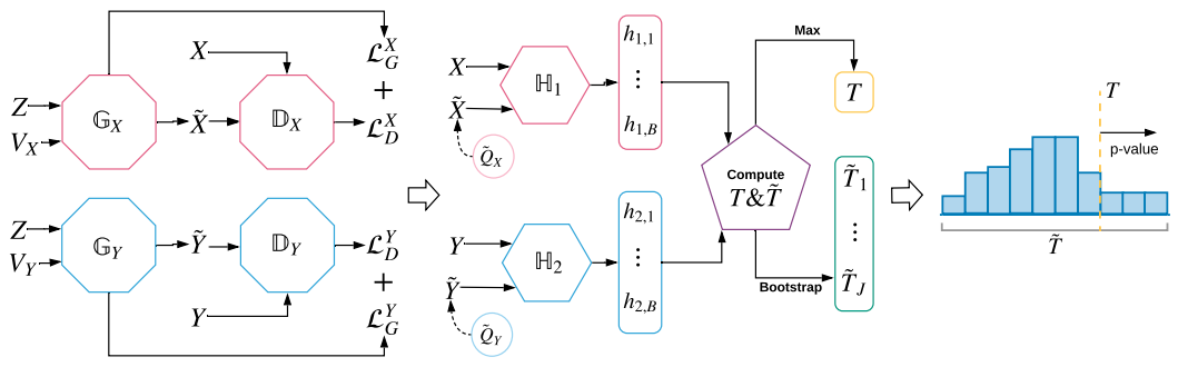
We give a graphical overview of our proposed testing procedure in Figure 1. We first employ double GANs to compute the test statistic that is the maximum of the GCMs over multiple transform functions. We then employ multiplier bootstrap to compute the corresponding -value. We next detail the main components of our testing procedure.
3.1 Test statistic
We begin with two function spaces, and , indexed by some parameters and , respectively. In our implementation, we set and to the classes of neural networks with a single-hidden layer, finitely many hidden nodes, and the sigmoid activation function. However, a broad range of other function spaces may be considered, as appropriate for the application at hand. We next randomly generate functions, , , where we independently generate i.i.d. multivariate normal variables , and . We then set , and , . Consider the following maximum-type test statistic,
where is the sampling variance estimator,
To compute , we need to estimate the conditional means, and , which can be done by applying some supervised learning methods. However, this needs to be performed for all . In theory, should diverge to infinity to guarantee the power property of the test. As such, this approach is computationally very expensive. Instead, we propose to implement this step based on the generators and estimated using GANs, which is much more efficient computationally.
Specifically, we first randomly generate i.i.d. samples , from multivariate normal distribution, for . We then feed and into GANs to obtain the pseudo samples , and feed and to obtain , for . These pseudo samples approximate the conditional distribution of and given , respectively. We then compute
for . Plugging the estimated means into produces the sample test statistic,
| (4) | |||
To help reduce the type-I error, we further employ a data splitting and cross-fitting strategy, which has been commonly used in statistical inferences in recent years (Romano and DiCiccio, 2019). That is, we use different subsets of data samples to learn GANs and to construct the test statistic. We begin by dividing the data into folds of equal size. We use to denote the set of indices of subsamples in the th fold, and its complement. We next learn two generators and , based on and , to approximate the conditional distributions of and , for . Finally, for each and , we generate the pseudo samples and using and , and construct as in (4). In this way, and are conditionally independent of the observations in given . Such a cross-fitting strategy allows us to derive the asymptotic properties of the test under minimal conditions on the generators.
We summarize our procedure of computing the test statistic in Algorithm 1.
3.2 Approximation of conditional distribution via GANs
There are numerous GANs methods available for learning high-dimensional distributions. We adopt the proposal of Genevay et al. (2017) to learn the conditional distributions and in our setting thanks to its competitive performance. Recall that is the distribution of pseudo outcome generated by the generator given . We consider estimating by optimizing
Here denotes the Sinkhorn loss function between two probability measures with respect to some cost function and some regularization parameter ,
where is a set containing all probability measures whose marginal distributions correspond to and , is the Kullback-Leibler divergence, and is the product measure of and . When , measures the optimal transport of into with respect to the cost function (Cuturi, 2013). When , an entropic regularization is added to this optimal transport. As such, the objective function is a regularized optimal transport metric, and the regularization is to facilitate the computation, so that can be efficiently evaluated.
Intuitively, the closer the two probability measures, the smaller the Sinkhorn loss. As such, maximizing the loss with respect to the cost function learns a discriminator that can better discriminate the samples generated between and . On the other hand, minimizing the maximum cost with respect to the generator makes it closer to the true distribution . This yields the minimax formulation that we target. In practice, we approximate the cost and the generator based on neural networks. Integrations in the objective function are approximated by sample averages. The conditional distribution of is estimated similarly.
3.3 Bootstrap for the -value
Next, we propose a multiplier bootstrap method to approximate the distribution of under and compute the corresponding -value. Let . The key observation is that are asymptotically multivariate normal with zero mean under ; see the proof of Theorem 4 for details. Consequently, is to converge to a maximum of normal variables in absolute values.
To approximate this limiting distribution, we first estimate the covariance matrix of a -dimensional vector formed by using the sample covariance matrix , whose th entry is given by
We then generate i.i.d. random vectors with the covariance matrix equal to . This can be achieved by generating i.i.d. standard normal variables for and , then compute -dimensional normal random vectors whose th entry is given by for . We next compute , for , where is the maximum element of a vector in absolute value, and is the number of bootstrap samples. Finally, we use these maximum absolute values to approximate the distribution of under the null hypothesis. This yields the -value, . We summarize this bootstrap procedure in Algorithm 2.
4 Asymptotic theory
To derive the theoretical properties of the test statistic , we first introduce the concept of the “oracle” test statistic . If and were known a priori, then one can draw and from and directly, and can compute the test statistic by replacing and with and . We call the resulting an “oracle” test statistic. We next establish the double-robustness property of , which helps explain why our test can relax the requirement in (3). Roughly speaking, the double-robustness means that is asymptotically equivalent to when either the conditional distribution of , or that of , is well approximated by GANs. It guarantees that converges to at a faster rate than the estimated conditional distribution. In contrast, the convergence rate of the GCIT test statistic is the same as the rate of the estimated conditional distribution. For this reason, our procedure only requires a weaker condition.
Theorem 2 (Double-robustness)
Suppose is proportional to , and for some constant . Suppose for some constant . Then, , when
We note that the conditions on and are mild, as these are user-specified parameters. As we have mentioned, when both total variation distances converge to zero, the test statistic converges at a faster rate than those total variation distances. Therefore, we can greatly relax the condition in (3), and replace it with,
| (5) |
for some constants and any , where and denote the conditional distributions approximated via GANs trained on the -th subset of data samples. The next theorem summarizes this discussion.
Since , the convergence rate of is faster than that in (5). To ensure , it suffices to require . In contrast to (3), this rate is achievable. We consider two examples in Berrett et al. (2019) to illustrate this, while the condition holds in a much wider range of settings.
Example 3 (Parametric setting)
Suppose the parametric forms of and are correctly specified. Then under certain regularity conditions, the requirement holds if and for some , where and are the dimensions of the parameters defining the parametric models for and , respectively.
Example 4 (Nonparametric setting with binary data)
Suppose are binary variables. Then the requirement holds if the mean squared prediction errors of the nonparametric estimators of the conditional means of and given are and for some , , such that .
We briefly remark that, there is no explicit specification on in the statement of Theorem 3. It is implicitly imposed due to the requirement that , and is allowed to diverge with the sample size. In addition, the condition can be further relaxed to using the theory of higher order influence functions (Robins et al., 2008, 2017; Mukherjee et al., 2017). However, the resulting estimators would be considerably much more complicated, and thus we do not pursue those estimators.
Next, we show that our proposed test can control the type-I error asymptotically.
Theorem 4
Next, to derive the asymptotic power of the test, we introduce the pair of hypotheses based on the notion of weak conditional independence (Daudin, 1980),
where and denote the class of all squared integrable functions of and , respectively. We note that conditional independence implies weak conditional independence, i.e., implies , and implies . We consider an example to further elaborate on the difference between weak CI and CI.
Example 5
Let be binary random variables with the distribution functions,
and takes the value with equal probability. We can show that, for any ,
By definition, this implies that and are weakly conditionally independent given , since
However, , since the former equals , and the latter equals . As such, and are not conditionally independent given .
The next theorem shows that our proposed test is consistent against the alternatives in , but not against all alternatives in .
Theorem 5
Finally, we remark that our test is constructed based on . Meanwhile, we may consider another test based on , where is the joint distribution of , , and is a neural network class of functions of . This type of test is consistent against all alternatives in . However, in our numerical experiments, we find it less powerful compared to our test. This agrees with the observation by Li and Fan (2019) in that, even though the tests based on weak CI cannot fully characterize CI, they potentially enjoy an improved power.
5 Numerical studies
We begin with a discussion of some implementation details. We then carry out simulations to study the empirical size and power of the proposed test, and compare with several alternative methods. We further illustrate with an application to a cancer genetics example.
5.1 Implementation details
For the number of functions in Algorithm 2, it represents a trade-off. By Theorem 5, should be as large as possible to guarantee a good power. In practice, the computation complexity increases as increases. Our numerical studies suggest that the value of between and achieves a good balance between the power and the computational cost, and we fix . For the number of pseudo samples , and the number of sample splittings , we find the results are not overly sensitive to their choices, and thus we fix and . Besides, we set the number of bootstrap samples .
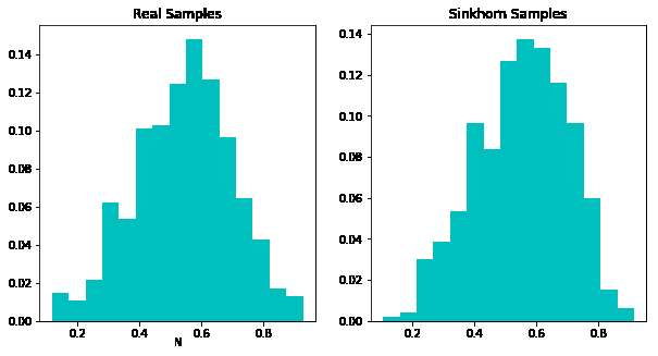
For the GANs, we use a single-hidden layer neural network to approximate both the discriminator and the generator. The number of nodes in the hidden layer is set at . The dimension of the input noise and is set at . These tuning parameters are chosen following the common practice in the GANs literature, and also by investigating the goodness-of-fit of the resulting generator, which can be done by comparing the conditional histogram of the generated samples to that of the true samples. In our experiments, we find such an approach yields GANs with satisfactory performances. More specifically, let denote the dimension of , and the sample average . Let denote a simulated sample to approximate the distribution of obtained by the generator . When is accurate, we expect the conditional distribution of and given are similar. As such, for any -dimensional vector , the histograms and should be similar. We sample i.i.d. vectors from . For each , we plot the histogram and . See Figures 2 (a) and (b) for the conditional histograms with two choices of . It is seen that the GANs fit the conditional density reasonably well. The fitted conditional distribution for can be checked in a similar fashion.
 |
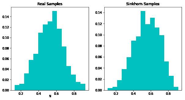 |
| (a) One random value of | (b) Another random value of |
5.2 Simulations
We generate the data following the post nonlinear noise model similarly as in Zhang et al. (2011); Doran et al. (2014); Bellot and van der Schaar (2019), i.e.,
The entries of are randomly and uniformly sampled from , then normalized to the unit norm. The noise variables are independently sampled from a normal distribution with mean zero and variance . In this model, the parameter determines the degree of conditional dependence. When , holds, and otherwise holds. The sample size is set at .
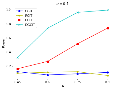
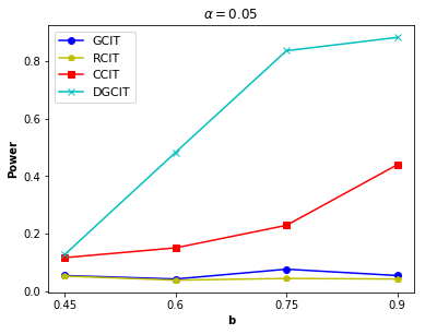
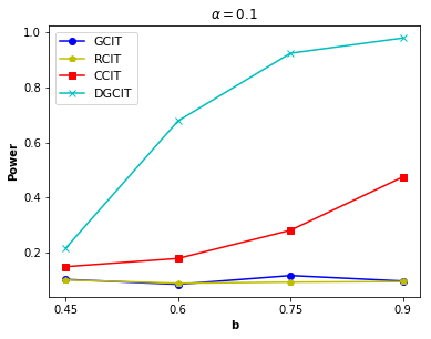
We call our test DGCIT, short for double GANs-based conditional independence test. We compare it with the GCIT test of Bellot and van der Schaar (2019), the regression-based test (RCIT) of Shah and Peters (2018), the kernel MMD-based test (KCIT) of Zhang et al. (2011), and the classifier CI test (CCIT) of Sen et al. (2017).
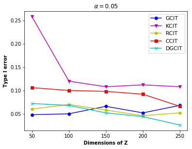
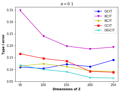
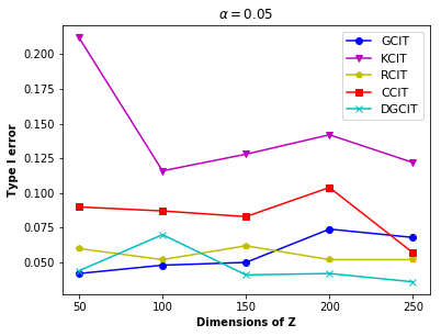
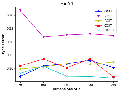
We first study the empirical size when . We vary the dimension of as , and consider two generation distributions. We first generate from a standard normal distribution, then from a Laplace distribution. We set the significance level at and . Figure 3 reports the empirical size of the tests aggregated over 500 data replications. We make the following observations. First, the type-I error rates of our test and RCIT are close to or below the nominal level in nearly all cases. Second, KCIT fails in that its type-I error is considerably larger than the nominal level in all cases. We suspect it is due to the high-dimensional setting where . We have experimented with , and found that KCIT is able to control the type-I error in that case. This is consistent with Proposition 5 of Zhang et al. (2011), which suggests that KCIT should work in a low-dimensional setting. Third, GCIT and CCIT both have inflated type-I errors in some cases. Take GCIT as an example. When is normal, and , its empirical size is close to . This is consistent with our discussion in Section 2.1, since GCIT requires a rather strong condition to control the type-I error.
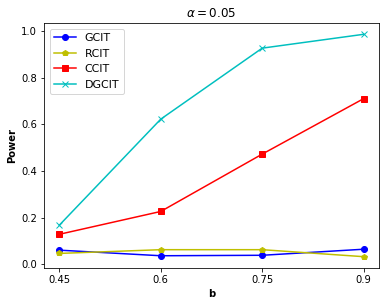
We then study the empirical power when . We generate from a standard normal distribution, with , and vary the value of that controls the magnitude of the alternative. Figure 4 reports the empirical power of the tests over 500 data replications. We observe that our test is the most powerful, and the empirical power approaches 1 as increases to , demonstrating the consistency of the test. Meanwhile, both GCIT and RCIT have no power in all cases. We do not report the power of KCIT, because as we have shown earlier, it cannot control the size, and thus its empirical power is not meaningful.
Finally, we discuss the computation time. All experiments were run on a 16 N1 CPUs Google Cloud Computing platform. The wall clock time for running the entire GCIT test for one data replication was about 2.5 minutes. In contrast, the running time for CCIT was about 2 minutes, for KCIT about 30 seconds, and for GCIT and RCIT about 20 seconds.
5.3 Anti-cancer drug data example
We illustrate our proposed test with an anti-cancer drug dataset from the Cancer Cell Line Encyclopedia (Barretina et al., 2012). We concentrate on a subset, the CCLE data, that measures the treatment response of drug PLX4720. It is well known that the patient’s cancer treatment response to drug can be strongly influenced by alterations in the genome (Garnett et al., 2012). This data measures 1638 genetic mutations of cell lines, and the goal of our analysis is to determine which genetic mutation is significantly correlated with the drug response after conditioning on all other mutations. The same data was also analyzed in Tansey et al. (2018) and Bellot and van der Schaar (2019). We adopt the same screening procedure as theirs to screen out irrelevant mutations, which leaves a total of 466 potential mutations for our conditional independence testing.
| BRAF.V600E | BRAF.MC | HIP1 | FTL3 | CDC42BPA | THBS3 | DNMT1 | PRKD1 | PIP5K1A | MAP3K5 | |
| EN | 1 | 3 | 4 | 5 | 7 | 8 | 9 | 10 | 19 | 78 |
| RF | 1 | 2 | 3 | 14 | 8 | 34 | 28 | 18 | 7 | 9 |
| GCIT | 0.001 | 0.001 | 0.008 | 0.521 | 0.050 | 0.013 | 0.020 | 0.002 | 0.001 | 0.001 |
| DGCIT | 0 | 0 | 0 | 0 | 0 | 0 | 0 | 0 | 0 | 0.794 |
The ground truth is unknown for this data. Instead, we compare with the variable importance measures obtained from fitting an elastic net (EN) model and a random forest (RF) model as reported in Barretina et al. (2012). In addition, we compare with the GCIT test of Bellot and van der Schaar (2019). Table 1 reports the corresponding variable importance measures and the -values, for 10 mutations that were also reported by Bellot and van der Schaar (2019). We see that, the -values of the tests generally agree well with the variable important measures from the EN and RF models. Meanwhile, the two conditional independence tests agree relatively well, except for two genetic mutations, MAP3K5 and FTL3. GCIT concluded that MAP3K5 is significant () but FTL3 is not (), whereas our test leads to the opposite conclusion that MAP3K5 is insignificant () but FTL3 is (). Besides, both EN and RF place FTL3 as an important mutation. We then compare our findings with the cancer drug response literature. Actually, MAP3K5 has not been previously reported in the literature as being directly linked to the PLX4720 drug response. Meanwhile, there is strong evidence showing the connections of the FLT3 mutation with cancer response (Tsai et al., 2008; Larrosa-Garcia and Baer, 2017). Combining the existing literature with our theoretical and synthetic results, we have more confidence about the findings of our proposed test.
6 Discussion
In this article, we have developed a new inferential procedure for high-dimensional conditional independence testing, where the dimension of the conditional variables can diverge with the sample size. Our proposal utilizes a set of state-of-the-art deep learning tools to help address a classical statistics and machine learning problem. It integrates GANs, neural networks, cross-fitting and multiplier bootstrap. It achieves the asymptotic guarantees under much weaker conditions, and enjoys better empirical performances, when compared to the existing tests. As a tradeoff, our test is computationally more complicated. Nevertheless, the wall clock time for running the entire test for one data replication is in the order of a few minutes and is deemed reasonable. Finally, the computer code is publicly available on the GitHub repository: https://github.com/tianlinxu312/dgcit.
A Proofs
We provide the proofs of Proposition 1, Theorems 3, 4, and 5. We omit the proof of Theorem 2, since it is similar to that of Theorem 3. We note that Theorems 2-5 are established under our choice of the function classes and , which are set to the classes of neural networks with a single-hidden layer, finitely many hidden nodes, and the sigmoid activation function, as used in our implementation. Meanwhile, our results can be extended to more general choices of the function classes.
A.1 Proof of Proposition 1
Note that the total variation distance is bounded by . Suppose . Then we have . By the dominated convergence theorem, we have .
By Theorem 1.2 of Devroye et al. (2018), we have is proportional to
It follows that
Applying Theorem 1.2 of Devroye et al. (2018) again, we obtain that is proportional to
Therefore, we obtain that,
Since the data is exchangeable, we have that,
| (8) |
Next, we show (8) is violated in the linear regression example. By the data exchangeability, it suffices to show is not . With some calculations, we obtain that,
| (9) | ||||
By the definition of , we have
where consist of i.i.d. copies of defined in Example 1. It follows that,
| (10) |
where is the dimension of .
Next, we show that,
| (11) |
or equivalently,
We have already shown that . By the dominated convergence theorem, it suffices to show that,
By definition, it in turn suffices to show that,
This holds by Markov’s inequality, as
This completes the proof of Proposition 1.
A.2 Proof of Theorem 3
We begin by providing an upper bound for the function classes and . Recall that both and are classes of neural networks with a single-hidden layer, finitely many hidden nodes, and the sigmoid activation function. Because of that, each function and can be represented as
where and correspond to the sets of parameters and , respectively, and is a finite integer. Note that the sigmoid function is bounded. As such, the functions and are uniformly bounded by and , respectively. Since we sample many functions and , these functions are uniformly bounded by
Since these parameters are sampled from standard normal distributions, and that
for any , we can show that is upper bounded by , with probability approaching one. Note that grows polynomially with respect to the sample size . Therefore, we have that the functions in and are upper bounded by in absolute values.
Define a test statistic
where the is constructed based on and , instead of and . It suffices to show that , and .
Step 1. We first consider the difference . For any sequences , , we have that,
| (12) |
Consequently, we have , where
If for some constant , then it suffices to show that , for , where
The number of folds is finite, as such, it suffices to show that , for and , where
We divide the rest of the proof into four sub-steps. We first show that , for . Finally, we show for some constant .
Step 1.1. Recall we have shown that the functions in and are bounded by in absolute values at the beginning of the proof of Theorem 3. By Bernstein’s inequality, we have that,
for any and . Set , where the constant is as defined in the statement of Theorem 2. For a sufficiently large , we have . It follows that
By Bonferroni’s inequality, we obtain that,
Under the condition , we obtain with probability that,
| (13) |
as is proportional to , and denotes some positive constant.
Similarly, we can show that,
with probability . Combining this with (13), we obtain with probability that,
| (14) | ||||
Conditional on , the expectation of equals zero. Under the null hypothesis, the expectation of equals zero as well. Applying Bernstein’s inequality again, we can show with probability tending to that,
| (15) |
where
Let denote the event in (14). The last term on the second line can be bounded from above by
| (16) | |||||
| (17) |
Since is proportional to , by (12), (16) is upper bounded by
By the boundedness of the function class , it can be further bounded from above by
| (18) |
The above quantity is of order . Consequently, (16) is of the order .
Note that the event occurs with probability at least . By the boundedness of the function class , (17) is of the order .
Therefore, is of the order . This implies that can be bounded from above by , which in turn yields that , since .
Step 1.2. This step can be proven in a similar way as Step 1.1, and is omitted.
Step 1.3. Under , the expectation of
equals
Similar to (18), its absolute value can be upper bounded by
Following Cauchy-Schwarz inequality, we have that,
This yields that,
Following similar arguments as in Step 1.1, we obtain that,
Therefore, we obtain that .
Step 1.4. Recall that is defined by
With some calculations, it is equal to
| (19) |
where the estimated conditional expectation is computed using GANs.
Consider the second term in (19). Following similar arguments as in Steps 1.1 and 1.3, we have that,
where equals
Similar to (14), we can show that,
Consequently, we have that,
Since the function classes and are bounded, both GCM and GCM∗ are bounded by in absolute values. Consequently,
| (20) |
Next, consider the first term in (19). Note that it can be represented by
Similar to (14), we can show that,
Following similar arguments as in Steps 1.1 and 1.3, we can show that,
for some constant . It follows that,
and henceforth,
Combining this together with (20) yields that,
Then, we have that,
for some constant . Therefore, we have that
with probability tending to .
Step 2. We next consider the difference , and show that it is of the order . Denote by the variance estimator with and replaced by and . Using (12), the difference between and is upper bounded by
Under , similar to (14), we can show that,
To show , it suffices to show that for some constant . Since both and are bounded away from zero, it suffices to show that .
Following similar arguments as in Steps 1.1 and 1.3, we can show that,
This completes the proof of Theorem 3.
A.3 Proof of Theorem 4
In the proof of Theorem 3, we have already shown that . Following similar arguments as in Step 1.4, we can show that , where
where
By (13), following similar arguments as in the proof regarding the term in Theorem 3, we can show that , where
Similarly, we can show that , where
Therefore, we have shown that . Since , we have that,
| (21) |
Define a matrix whose th entry is given by
In the following, we show that,
| (22) |
When is finite, this is implied by the classical weak convergence results. When diverges with , we require for some constant . By the definition of , the variance of
is bounded from above by . Moreover, combining the boundedness of the function spaces and together with the definition of yields that,
are uniformly bounded from infinity by , with probability tending to . We can show that (22) holds. This implies that,
is asymptotically normal with zero mean.
Combining (22) together with (21) yields that,
| (23) |
for any sufficiently small , where the little-o terms are uniform in .
Following similar arguments as in Step 1.4 and Step 2 of the proof of Theorem 3, we can show that for some constant . Following similar arguments for (23), we have that,
for any sufficiently small . Since the little-o terms are uniform in , we obtain that,
By Theorem 1 of Chernozhukov et al. (2017), the term on the second line can be bounded by , where denotes some positive constant. Since , . As grows to zero, this term becomes negligible. Consequently, we obtain that,
As such, the distribution of our test statistic can be well-approximated by that of the bootstrap samples. This completes the proof of Theorem 4.
A.4 Proof of Theorem 5
We break the proof into two steps. In Step 1, we show that, under , there exist two neural networks functions and , such that
In Step 2, we prove the power of our test approaches one, as the sample size diverges to infinity.
Step 1. We first observe that the measure is continuous in and . That is, for any and , the difference decays to zero as both and decay to zero.
Under , there exist functions and , such that . Without loss of generality, assume and are bounded. Otherwise, we can find sequences of bounded functions and that converge to and under -norm, respectively. As a result, we would have for some .
By Lusin’s theorem, we can find a sequence of bounded and continuous functions , such that . By dominated convergence theorem, it follows that converges to under -norm. Similarly, we can find a sequence of continuous functions , such that converges to under -norm. This together with the fact that is continuous in implies that there exist some continuous functions and , such that .
A key observation here is that, the class of neural networks have universal approximation property. Since the support of and are bounded, it follows from Theorem 1 of Cybenko (1989) that the class of single-layered neural networks with sigmoid activation function is dense in the class of bounded, continuous functions with a compact support. As such, we can find some neural network functions and such that . We then argue that there must exist and , such that . Otherwise, and can be represented as linear combinations of neural network functions in , with finitely many number of parameters, and we would have as a result. This completes Step 1.
Step 2. We first show that is a Lipschitz continuous function of . Note that and are Lipschitz continuous functions of and , respectively. For any , , we have that,
| (24) | ||||
| (25) |
Since the class of functions in are upper bounded by with probability tending to , the right-hand-side of (24) is bounded from above by
with probability tending to . By Jensen’s inequality, the above quantity can be further bounded from above by
for some constant . Following similar arguments, we can show that the right-hand-side of (25) is bounded from above by , for any and , with probability tending to . To summarize, conditional on the event that and are bounded function classes, we have shown that
Consequently, for any sufficiently small , there exists a neighborhood for some constant around , such that for any that belongs to this neighborhood.
Since are generated from the multivariate normal distribution, and the dimensions and are finite, the probability that belongs to this neighborhood is strictly greater than for some constant . Since , the probability that at least one pair of parameters belongs to this neighborhood approaches one. Consequently, we have that,
with probability tending to .
Following similar arguments as in the proof of Theorems 3 and 4, we can show that , and . Consequently, both probabilities and converge to zero. Therefore, the probability that the -value is greater than is bounded by the probability that , which converges to zero. This completes the proof of Theorem 5.
References
- Barretina et al. (2012) Jordi Barretina, Giordano Caponigro, Nicolas Stransky, Kavitha Venkatesan, Adam A Margolin, Sungjoon Kim, Christopher J Wilson, Joseph Lehár, Gregory V Kryukov, Dmitriy Sonkin, et al. The cancer cell line encyclopedia enables predictive modelling of anticancer drug sensitivity. Nature, 483(7391):603–607, 2012.
- Bellot and van der Schaar (2019) Alexis Bellot and Mihaela van der Schaar. Conditional independence testing using generative adversarial networks. In Advances in Neural Information Processing Systems, pages 2199–2208, 2019.
- Bergsma (2004) Wicher Pieter Bergsma. Testing conditional independence for continuous random variables. Eurandom, 2004.
- Berrett et al. (2019) Thomas B Berrett, Yi Wang, Rina Foygel Barber, and Richard J Samworth. The conditional permutation test for independence while controlling for confounders. Journal of the Royal Statistical Society: Series B (Statistical Methodology), accepted, 2019.
- Candes et al. (2018) Emmanuel Candes, Yingying Fan, Lucas Janson, and Jinchi Lv. Panning for gold:‘model-x’knockoffs for high dimensional controlled variable selection. Journal of the Royal Statistical Society: Series B (Statistical Methodology), 80(3):551–577, 2018.
- Chen et al. (2020) Minshuo Chen, Wenjing Liao, Hongyuan Zha, and Tuo Zhao. Statistical guarantees of generative adversarial networks for distribution estimation. arXiv preprint arXiv:2002.03938, 2020.
- Chernozhukov et al. (2017) Victor Chernozhukov, Denis Chetverikov, and Kengo Kato. Detailed proof of nazarov’s inequality. arXiv preprint arXiv:1711.10696, 2017.
- Cuturi (2013) Marco Cuturi. Sinkhorn distances: Lightspeed computation of optimal transport. In Advances in neural information processing systems, pages 2292–2300, 2013.
- Cybenko (1989) George Cybenko. Approximation by superpositions of a sigmoidal function. Mathematics of control, signals and systems, 2(4):303–314, 1989.
- Daudin (1980) JJ Daudin. Partial association measures and an application to qualitative regression. Biometrika, 67(3):581–590, 1980.
- Devroye et al. (2018) Luc Devroye, Abbas Mehrabian, and Tommy Reddad. The total variation distance between high-dimensional gaussians. arXiv preprint arXiv:1810.08693, 2018.
- Doran et al. (2014) Gary Doran, Krikamol Muandet, Kun Zhang, and Bernhard Schölkopf. A permutation-based kernel conditional independence test. In UAI, pages 132–141, 2014.
- Fukumizu et al. (2008) Kenji Fukumizu, Arthur Gretton, Xiaohai Sun, and Bernhard Schölkopf. Kernel measures of conditional dependence. In Advances in neural information processing systems, pages 489–496, 2008.
- Garnett et al. (2012) Mathew Garnett, Elena Edelman, Sonja Gill, Chris Greenman, Anahita Dastur, King Lau, Patricia Greninger, Richard Thompson, Xi Luo, Jorge Soares, Qingsong Liu, Francesco Iorio, Didier Surdez, Li Chen, Randy Milano, Graham Bignell, Ah Tam, Helen Davies, Jesse Stevenson, and Cyril Benes. Systematic identification of genomic markers of drug sensitivity in cancer cells. Nature, 483:570–5, 03 2012. doi: 10.1038/nature11005.
- Genevay et al. (2017) Aude Genevay, Gabriel Peyré, and Marco Cuturi. Learning generative models with sinkhorn divergences. arXiv preprint arXiv:1706.00292, 2017.
- Goodfellow et al. (2014) Ian Goodfellow, Jean Pouget-Abadie, Mehdi Mirza, Bing Xu, David Warde-Farley, Sherjil Ozair, Aaron Courville, and Yoshua Bengio. Generative adversarial nets. In Advances in neural information processing systems, pages 2672–2680, 2014.
- Gretton et al. (2012) Arthur Gretton, Karsten M Borgwardt, Malte J Rasch, Bernhard Schölkopf, and Alexander Smola. A kernel two-sample test. Journal of Machine Learning Research, 13(Mar):723–773, 2012.
- Gui et al. (2020) Jie Gui, Zhenan Sun, Yonggang Wen, Dacheng Tao, and Jieping Ye. A review on generative adversarial networks: Algorithms, theory, and applications. arXiv preprint arXiv:2001.06937, 2020.
- Hoyer et al. (2009) Patrik O Hoyer, Dominik Janzing, Joris M Mooij, Jonas Peters, and Bernhard Schölkopf. Nonlinear causal discovery with additive noise models. In Advances in neural information processing systems, pages 689–696, 2009.
- Imaizumi and Fukumizu (2019) Masaaki Imaizumi and Kenji Fukumizu. Deep neural networks learn non-smooth functions effectively. In The 22nd international conference on artificial intelligence and statistics, pages 869–878. PMLR, 2019.
- Koller and Friedman (2009) D. Koller and N. Friedman. Probabilistic Graphical Models: Principles and Techniques. Adaptive computation and machine learning. MIT Press, 2009.
- Larrosa-Garcia and Baer (2017) Maria Larrosa-Garcia and Maria R. Baer. Flt3 inhibitors in acute myeloid leukemia: Current status and future directions. Molecular Cancer Therapeutics, 16(6):991–1001, 2017.
- Li (2018) Bing Li. Sufficient Dimension Reduction: Methods and Applications with R. CRC Press, 2018.
- Li and Fan (2019) Chun Li and Xiaodan Fan. On nonparametric conditional independence tests for continuous variables. Wiley Interdisciplinary Reviews: Computational Statistics, page e1489, 2019.
- Liang (2018) Tengyuan Liang. On how well generative adversarial networks learn densities: Nonparametric and parametric results. arXiv preprint arXiv:1811.03179, 2018.
- Mukherjee et al. (2017) Rajarshi Mukherjee, Whitney K Newey, and James M Robins. Semiparametric efficient empirical higher order influence function estimators. arXiv preprint arXiv:1705.07577, 2017.
- Pan et al. (2017) Wenliang Pan, Xueqin Wang, Canhong Wen, Martin Styner, and Hongtu Zhu. Conditional local distance correlation for manifold-valued data. In International Conference on Information Processing in Medical Imaging, pages 41–52. Springer, 2017.
- Pearl (2009) Judea Pearl. Causality: Models, Reasoning and Inference. Cambridge: Cambridge University Press, 2nd Edition, 2009.
- Robins et al. (2008) James Robins, Lingling Li, Eric Tchetgen, Aad van der Vaart, et al. Higher order influence functions and minimax estimation of nonlinear functionals. In Probability and statistics: essays in honor of David A. Freedman, pages 335–421. Institute of Mathematical Statistics, 2008.
- Robins et al. (2017) James M Robins, Lingling Li, Rajarshi Mukherjee, Eric Tchetgen Tchetgen, Aad van der Vaart, et al. Minimax estimation of a functional on a structured high-dimensional model. The Annals of Statistics, 45(5):1951–1987, 2017.
- Romano and DiCiccio (2019) J Romano and Cyrus DiCiccio. Multiple data splitting for testing. Technical report, Stanford University, 2019.
- Sen et al. (2017) Rajat Sen, Ananda Theertha Suresh, Karthikeyan Shanmugam, Alexandros G Dimakis, and Sanjay Shakkottai. Model-powered conditional independence test. In Advances in neural information processing systems, pages 2951–2961, 2017.
- Shah and Peters (2018) Rajen D Shah and Jonas Peters. The hardness of conditional independence testing and the generalised covariance measure. arXiv preprint arXiv:1804.07203, 2018.
- Su and White (2007) Liangjun Su and Halbert White. A consistent characteristic function-based test for conditional independence. Journal of Econometrics, 141(2):807–834, 2007.
- Su and White (2014) Liangjun Su and Halbert White. Testing conditional independence via empirical likelihood. Journal of Econometrics, 182(1):27–44, 2014.
- Tansey et al. (2018) Wesley Tansey, Victor Veitch, Haoran Zhang, Raul Rabadan, and David M Blei. The holdout randomization test: Principled and easy black box feature selection. arXiv preprint arXiv:1811.00645, 2018.
- Tsai et al. (2008) James Tsai, John T. Lee, Weiru Wang, et al. Discovery of a selective inhibitor of oncogenic b-raf kinase with potent antimelanoma activity. Proceedings of the National Academy of Sciences, 105(8):3041–3046, 2008. doi: 10.1073/pnas.0711741105.
- Wang et al. (2018) Xia Wang, Yongmiao Hong, et al. Characteristic function based testing for conditional independence: a nonparametric regression approach. Econometric Theory, 34(4):815–849, 2018.
- Wang et al. (2015) Xueqin Wang, Wenliang Pan, Wenhao Hu, Yuan Tian, and Heping Zhang. Conditional distance correlation. Journal of the American Statistical Association, 110(512):1726–1734, 2015.
- Zhang et al. (2011) K Zhang, J Peters, D Janzing, and B Schölkopf. Kernel-based conditional independence test and application in causal discovery. In 27th Conference on Uncertainty in Artificial Intelligence (UAI 2011), pages 804–813. AUAI Press, 2011.