Tensor Factor Model Estimation by Iterative Projection

Supplementary Material to “Tensor Factor Model Estimation by Iterative Projection”

Abstract

Tensor time series, which is a time series consisting of tensorial observations, has become ubiquitous. It typically exhibits high dimensionality. One approach for dimension reduction is to use a factor model structure, in a form similar to Tucker tensor decomposition, except that the time dimension is treated as a dynamic process with a time dependent structure. In this paper we introduce two approaches to estimate such a tensor factor model by using iterative orthogonal projections of the original tensor time series. These approaches extend the existing estimation procedures and improve the estimation accuracy and convergence rate significantly as proven in our theoretical investigation. Our algorithms are similar to the higher order orthogonal projection method for tensor decomposition, but with significant differences due to the need to unfold tensors in the iterations and the use of autocorrelation. Consequently, our analysis is significantly different from the existing ones. Computational and statistical lower bounds are derived to prove the optimality of the sample size requirement and convergence rate for the proposed methods. Simulation study is conducted to further illustrate the statistical properties of these estimators.

, , , and

1 Introduction

Motivated by a diverse range of modern scientific applications, analysis of tensors, or multi-dimensional arrays, has emerged as one of the most important and active research areas in statistics, computer science, and machine learning. Large tensors are encountered in genomics (Alter and Golub, 2005, Omberg, Golub and Alter, 2007), neuroimaging analysis (Zhou, Li and Zhu, 2013, Sun and Li, 2017), recommender systems (Bi, Qu and Shen, 2018), computer vision (Liu et al., 2012), community detection (Anandkumar et al., 2014), among others. High-order tensors often bring about high dimensionality and impose significant computational challenges. For example, functional MRI produces a time series of 3-dimensional brain images, typically consisting of hundreds of thousands of voxels observed over time. Previous work has developed various tensor-based methods for independent and identically distributed (i.i.d.) tensor data or tensor data with i.i.d. noise. However, as far as we know, the statistical framework for general tensor time series data was not well studied in the literature.

Factor analysis is one of the most useful tools for understanding common dependence among multi-dimensional outputs. Over the past decades, vector factor models have been extensively studied in the statistics and economics communities. For instance, Chamberlain and Rothschild (1983), Bai and Ng (2002), Stock and Watson (2002) and Bai (2003) developed the static factor model using principal component analysis (PCA). They assumed that the common factors must have impact on most of the time series, and weak serial dependence is allowed for the idiosyncratic noise process. Fan, Liao and Mincheva (2011, 2013), Fan, Liu and Wang (2018) established large covariance matrix estimation based on the static factor model. The static factor model has been further extended to the dynamic factor model in Forni et al. (2000). The latent factors are assumed to follow a time series process, which is commonly taken to be a vector autoregressive process. Fan, Liao and Wang (2016) studied semi-parametric factor models through projected principal component analysis. Pena and Box (1987), Pan and Yao (2008), Lam, Yao and Bathia (2011) and Lam and Yao (2012) adopted another type of factor model. They assumed that the latent factors capture all dynamics of the observed process, and thus the idiosyncratic noise process has no serial dependence. We will adopt this approach. We note that the factor process may have complex dynamic behavior, resulting in complex dynamics of the observed tensor, even with white additive noise process. Of course, when all the dynamics of the observed tensor process are ‘forced’ to be included in the signal process induced by the factor process, situations may arise in which some factors are ‘weak’ (or have impact on a small portion of the observed series in the tensor). This leads us to consider the ‘signal strength’ in our investigation.

Although there have been significant efforts in developing methodologies and theories for vector factor models, there is a paucity of literature on matrix- or tensor-valued time series. Wang, Liu and Chen (2019) proposed a matrix factor model for matrix-valued time series, which explores the matrix structure. Chen, Tsay and Chen (2020) established a general framework for incorporating domain and prior knowledge in the matrix factor model through linear constraints. Chen and Chen (2019) applied the matrix factor model to the dynamic transport network. Chen and Fan (2021) developed an inferential theory of the matrix factor model under a different setting from that in Wang, Liu and Chen (2019) .

Recently, Chen, Yang and Zhang (2021) introduced a factor approach for analyzing high dimensional dynamic tensor time series in the form

$${\cal X}_{t}={\cal M}_{t}+{\cal E}_{t},$$ (1.1)

where ${\cal X}_{1},...,{\cal X}_{T}\in\mathbb{R}^{d_{1}\times\cdots\times d_{K}}$ are the observed tensor time series, ${\cal M}_{t}$ and ${\cal E}_{t}$ are the corresponding signal and noise components of ${\cal X}_{t}$, respectively. The goal is to estimate the unknown signal tensor ${\cal M}_{t}$ from the tensor time series data. Following Lam and Yao (2012), it is assumed that the signal tensor accommodates all dynamics, making the idiosyncratic noise ${\cal E}_{t}$ uncorrelated (white) across time. It is further assumed that ${\cal M}_{t}$ lives in a lower dimensional space and has certain multilinear decomposition. Specifically, we assume that ${\cal M}_{t}$ satisfies a Tucker-type decomposition and model (1.1) can be written as

$${\cal X}_{t}={\cal F}_{t}\times_{1}A_{1}\times_{2}\ldots\times_{K}A_{K}+{\cal E}_{t},$$ (1.2)

where $A_{k}$ is the deterministic loading matrix of size $d_{k}\times r_{k}$ and $r_{k}\ll d_{k}$, and the core tensor ${\cal F}_{t}$ itself is a latent tensor factor process of dimension $r_{1}\times\ldots\times r_{K}$. Here the $k$-mode product of ${\cal X}\in\mathbb{R}^{d_{1}\times d_{2}\times\cdots\times d_{K}}$ with a matrix $U\in\mathbb{R}^{d_{k}^{\prime}\times d_{k}}$, denoted as ${\cal X}\times_{k}U$, is an order $K$-tensor of size $d_{1}\times\cdots\times d_{k-1}\times d_{k}^{\prime}\times d_{k+1}\times\cdots\times d_{K}$ such that

$$({\cal X}\times_{k}U)_{i_{1},...,i_{k-1},j,i_{k+1},...,i_{K}}=\sum_{i_{k}=1}^{d_{k}}{\cal X}_{i_{1},i_{2},...,i_{K}}U_{j,i_{k}}.$$

The core tensor ${\cal F}_{t}$ is usually much smaller than ${\cal X}_{t}$ in dimension. This structure provides an effective dimension reduction, as all the comovements of individual time series in ${\cal X}_{t}$ are driven by ${\cal F}_{t}$. Without loss of generality, assume that $A_{k}$ is of rank $r_{k}\ll d_{k}$. It should be noted that vector and matrix factor models can be viewed as special cases of our model since a vector time series is a tensor time series composed of a single fiber ($K=1$), and a matrix times series is one composed of a single slice ($K=2$).

Chen, Yang and Zhang (2021) proposed two estimation procedures, namely TOPUP and TIPUP, for estimating the column space spanned by the loading matrix $A_{k}$, for $k=1,\ldots,K$. The two procedures are based on different auto-cross-product operations of the observed tensors ${\cal X}_{t}$ to accumulate information, but they both utilize the assumption that the noise ${\cal E}_{t}$ and ${\cal E}_{t-h},~{}h>0$ are uncorrelated. The convergence rates of their estimators critically depend on $d=d_{1}d_{2}\ldots d_{K}$, a potentially very large number as $d_{k},~{}k=1,\ldots,K$, are large. Often a large $T$, the length of the time series, is required for accurate estimation of the loading spaces.

In this paper we propose extensions of the TOPUP and TIPUP procedures, motivated by the following observation. Suppose that the loading matrices $A_{k}$ are orthonormal with $A_{k}^{\top}A_{k}=I$, and we are given $A_{2},\ldots,A_{K}$. Let

$${\cal Z}_{t}={\cal X}_{t}\times_{2}A_{2}^{\top}\times_{3}\ldots\times_{K}A_{K}^{\top};\mbox{\ \ and \ \ }{\cal E}_{t}^{*}={\cal E}_{t}\times_{2}A_{2}^{\top}\times_{3}\ldots\times_{K}A_{K}^{\top};$$

Then (1.2) leads to

$${\cal Z}_{t}={\cal F}_{t}\times_{1}A_{1}+{\cal E}_{t}^{*}$$ (1.3)

where ${\cal Z}_{t}$ is a $d_{1}\times r_{2}\times\ldots\times r_{K}$ tensor. Since $r_{k}\ll d_{k}$, ${\cal Z}_{t}$ is a much smaller tensor than ${\cal X}_{t}$. Under proper conditions on the combined noise tensor ${\cal E}_{t}^{*}$, the estimation of the loading space of $A_{1}$ based on ${\cal Z}_{t}$ can be made significantly more accurate, as the convergence rate now depends on $d_{1}r_{2}\ldots r_{K}$ rather than $d_{1}d_{2}\ldots d_{K}$.

Of course, in practice we do not know $A_{2},\ldots,A_{K}$. Similar to backfitting algorithms, we propose an iterative algorithm. With a proper initial value, we iteratively estimate the loading space of $A_{k}$ at iteration $j$ based on

$${\cal Z}_{t,k}^{(j)}={\cal X}_{t}\times_{1}\widehat{A}_{1}^{(j)\top}\times_{2}\ldots\times_{k-1}\widehat{A}_{k-1}^{(j)\top}\times_{k+1}\widehat{A}_{k+1}^{(j-1)\top}\times_{k+2}\ldots\times_{K}\widehat{A}_{K}^{(j-1)\top},$$

using the estimate $\widehat{A}_{k^{\prime}}^{(j-1)},~{}k<k^{\prime}\leq K$ obtained in the previous iteration and the estimate $\widehat{A}_{k^{\prime}}^{(j)},~{}1\leq k^{\prime}<k$, obtained in the current iteration. Our theoretical investigation shows that the iterative procedures for estimating $A_{1}$ can achieve the convergence rate as if all $A_{2},\ldots,A_{K}$ are known and we indeed observe ${\cal Z}_{t}$ that follows model (1.3). We call the procedure iTOPUP and iTIPUP, based on the matrix unfolding mechanism used, corresponding to TOPUP and TIPUP procedures. To be more specific, our algorithms have two steps: (i) We first use the estimated column space of factor loading matrices of TOPUP (resp. TIPUP) to construct the initial estimate of factor loading spaces; (ii) We then iteratively perform matrix unfolding of the auto-cross-moments of much smaller tensors ${\cal Z}_{t,k}^{(j)}$ to obtain the final estimators.

We note that the iterative procedure is related to higher order orthogonal iteration (HOOI) that has been widely studied in the literature; see, e.g., De Lathauwer, De Moor and Vandewalle (2000), Sheehan and Saad (2007), Liu et al. (2014), Zhang and Xia (2018), among others. However, most of the existing works are not designed for tensor time series. They do not consider the special role of the time mode nor the covariance structure in the time direction. Typically HOOI treats the signal part as fixed or deterministic. In this paper we treat the signal as dynamic in the sense that the core tensor ${\cal F}_{t}$ in (1.2) is dynamic and the relationship between ${\cal F}_{t}$ and the lagged ${\cal F}_{t-h}$ is of interest. Our setting requires special treatment although each iteration of our iterative procedures also consists of power up and orthogonal projection operations. While HOOI applies the SVD directly to the matrix unfolding of the iteratively projected data, in our approach the SVD is applied to the matrix unfolding of the outer- and inner-auto-cross-product of the iteratively projected data, respectively in iTOPUP and iTIPUP. Although the iTOPUP algorithm proposed here can be reformulated as a twist of HOOI on the auto-cross-moment tensor, the iTIPUP algorithm is different and cannot be recast equivalently as HOOI. More importantly, the theoretical analysis and theoretical properties of the estimators are fundamentally different from those of HOOI, due to the dynamic structure of tensor time series and the need to use the auto-cross-product operation between the SVD and data projection in each iteration. Different concentration inequalities are derived to study the performance bounds.

In this paper, we establish upper bounds on the estimation errors for both the iTOPUP and the iTIPUP, which are much sharper than the respective theoretical guarantees for TOPUP and TIPUP, demonstrating the benefits of using iterative projection. It is also shown that the number of iterations needed for convergence is of order no greater than $\log(d)$. We mainly focus on the cases where the tensor dimensions are large and of similar order. We also cover the cases where the ranks of the tensor factor process increase with the dimensions of the tensor time series.

Chen, Yang and Zhang (2021) showed that the TIPUP has a faster convergence rate in estimation error than the TOPUP, under a mild condition on the level of signal cancellation. In contrast, the theoretically guaranteed rate of convergence for the iTOPUP in this paper is of the same order or even faster than that for the iTIPUP under certain regularity conditions. Our results also suggest an interesting phenomenon. Using the iterative procedures, we find that the increase in either dimension or sample size can improve the estimation of the factor loading space of the tensor factor model with the tensor order $K\geq 2$. We believe that such a super convergence rate is new in the literature. Specifically, under proper regularity conditions, the convergence rate of the iterative procedures for estimating the space of $A_{k}$ is $O_{\mathbb{P}}(T^{-1/2}d_{-k}^{-1/2})$, where $d_{-k}=\prod_{j\neq k}d_{j}$, while the existing rate for non-iterative procedures is $O_{\mathbb{P}}(T^{-1/2})$ for the vector factor model (Lam, Yao and Bathia, 2011) and the matrix/tensor factor models (Wang, Liu and Chen, 2019, Chen, Yang and Zhang, 2021). While the increase in the dimensions $d_{k}$ ($k=1,\ldots,K$) does not improve the performance of the non-iterative estimators, it significantly improves that of the proposed iterative estimators.

In addition, we establish the computational lower bound for the estimation of the loading spaces of tensor factor models under the hardness assumption of certain instances of hypergraphic planted clique detection problem. It shows that the sample size requirement (or signal to noise ratio condition) needed for using the TIPUP estimate as the initial values for the iterative procedures is unavoidable for any computationally manageable estimation procedure to achieve consistency, although the iterative procedures have faster convergence rates. Moreover, we provide a statistical lower bound which matches the rates of convergence of our iterative procedures under proper conditions.

Related work. We close this section by highlighting several recent papers on related topics. First, we draw attention to the work of Foster (1996), Fan, Liao and Wang (2016) and Chen et al. (2020). Chen et al. (2020) adopts a spectral initialization plus an iterative refinement step estimating procedure, so that our methods are related to theirs. However, due to the differences in problem setting and model assumptions, their estimation procedures, performance bounds and analytic techniques are all significantly different from ours. Foster (1996), Fan, Liao and Wang (2016) use the projection to the space spanned by the sieve bases without iteration. Rogers, Li and Russell (2013) assumes the tensor factor model in (1.2), with an additional specific AR structure on the dynamic of the factor process. The additional model structure led to an EM type of estimation approach, quite different from the approach we develop here. Wang, Zheng and Li (2021) concerns low rank tensor AR model and uses a nuclear norm penalty to enforce the low rank structure and optimization algorithms for estimation, again quite different from our approach.

The paper is organized as follows. Section 2.1 introduces basic notation and preliminaries of tensor analysis. We present the tensor factor model and the iTOPUP and iTIPUP procedures in Sections 2.2 and 2.3. Theoretical properties of the iTOPUP and iTIPUP are investigated in Section 3. Section 4 provides a brief summary. Numerical comparison of our iterative procedures and other methods, and all technical details are relegated to the Supplementary Material.

2 Tensor Factor Model by Orthogonal Iteration

2.1 Notation and preliminaries for tensor analysis

Throughout this paper, for a vector $x=(x_{1},...,x_{p})^{\top}$, define $\|x\|_{q}=(x_{1}^{q}+...+x_{p}^{q})^{1/q}$, $q\geq 1$. For a matrix $A=(a_{ij})\in\mathbb{R}^{m\times n}$, write the SVD as $A=U\Sigma V^{\top}$, where $\Sigma=\text{diag}(\sigma_{1}(A),\sigma_{2}(A),...,\sigma_{\min\{m,n\}}(A))$, with the singular values $\sigma_{1}(A)\geq\sigma_{2}(A)\geq\cdots\geq\sigma_{\min\{m,n\}}(A)\geq 0$ in descending order. The matrix spectral norm is denoted as $\|A\|_{\rm S}=\sigma_{1}(A).$ Let $\sigma_{\min}(A)$ (resp. $\sigma_{\max}(A)$) be the smallest (resp. largest) nontrivial singular value of $A$. For two sequences of real numbers $\{a_{n}\}$ and $\{b_{n}\}$, write $a_{n}=O(b_{n})$ (resp. $a_{n}\asymp b_{n}$) if there exists a constant $C$ such that $|a_{n}|\leq C|b_{n}|$ (resp. $1/C\leq a_{n}/b_{n}\leq C$) for all sufficiently large $n$, and write $a_{n}=o(b_{n})$ if $\lim_{n\to\infty}a_{n}/b_{n}=0$. Write $a_{n}\lesssim b_{n}$ (resp. $a_{n}\gtrsim b_{n}$) if there exist a constant $C$ such that $a_{n}\leq Cb_{n}$ (resp. $a_{n}\geq Cb_{n}$). Denote $a\wedge b=\min\{a,b\}$ and $a\vee b=\max\{a,b\}$. We use $C,C_{1},c,c_{1},...$ to denote generic constants, whose actual values may vary from line to line.

For any two $m\times r$ matrices with orthonormal columns, say, $U$ and $\widehat{U}$, suppose the singular values of $U^{\top}\widehat{U}$ are $\sigma_{1}\geq\sigma_{2}\geq\cdots\geq\sigma_{r}\geq 0$. A natural measure of distance between the column spaces of $U$ and $\widehat{U}$ is then

$$\|\widehat{U}\widehat{U}^{\top}-UU^{\top}\|_{\rm S}=\sqrt{1-\sigma_{r}^{2}},$$ (2.1)

which equals to the sine of the largest principle angle between the column spaces of $U$ and $\widehat{U}$.

For any two matrices $A\in\mathbb{R}^{m_{1}\times r_{1}},B\in\mathbb{R}^{m_{2}\times r_{2}}$, denote the Kronecker product $\odot$ as $A\odot B\in\mathbb{R}^{m_{1}m_{2}\times r_{1}r_{2}}$. For any two tensors ${\cal A}\in\mathbb{R}^{m_{1}\times m_{2}\times\cdots\times m_{K}},{\cal B}\in\mathbb{R}^{r_{1}\times r_{2}\times\cdots\times r_{N}}$, denote the tensor product $\otimes$ as ${\cal A}\otimes{\cal B}\in\mathbb{R}^{m_{1}\times\cdots\times m_{K}\times r_{1}\times\cdots\times r_{N}}$, such that

$$({\cal A}\otimes{\cal B})_{i_{1},...,i_{K},j_{1},...,j_{N}}=({\cal A})_{i_{1},...,i_{K}}({\cal B})_{j_{1},...,j_{N}}.$$

Let ${\rm{vec}}(\cdot)$ be the vectorization of matrices and tensors. The mode-$k$ unfolding (or matricization) is defined as ${\rm{mat}}_{k}({\cal A})$, which maps a tensor ${\cal A}$ to a matrix ${\rm{mat}}_{k}({\cal A})\in\mathbb{R}^{m_{k}\times m_{-k}}$ where $m_{-k}=\prod_{j\neq k}^{K}m_{j}$. For example, if ${\cal A}\in\mathbb{R}^{m_{1}\times m_{2}\times m_{3}}$, then

$$({\rm{mat}}_{1}({\cal A}))_{i,(j+m_{2}(k-1))}=({\rm{mat}}_{2}({\cal A}))_{j,(k+m_{3}(i-1))}=({\rm{mat}}_{3}({\cal A}))_{k,(i+m_{1}(j-1))}={\cal A}_{ijk}.$$

For tensor ${\cal A}\in\mathbb{R}^{m_{1}\times m_{2}\times\cdots\times m_{K}}$, the Hilbert Schmidt norm is defined as

$$\|{\cal A}\|_{{\rm HS}}=\sqrt{\sum_{i_{1}=1}^{m_{1}}\cdots\sum_{i_{K}=1}^{m_{K}}({\cal A})_{i_{1},...,i_{K}}^{2}}.$$

For a matrix, the Hilbert Schmidt norm is just the Frobenius norm. Define the tensor operator norm for an order-4 tensor ${\cal A}\in\mathbb{R}^{m_{1}\times m_{2}\times m_{3}\times m_{4}}$,

$$\|{\cal A}\|_{\rm{op}}=\max\left\{\sum_{i_{1},i_{2},i_{3},i_{4}}u_{i_{1},i_{2}}\cdot u_{i_{3},i_{4}}\cdot({\cal A})_{i_{1},i_{2},i_{3},i_{4}}:\|U_{1}\|_{\rm HS}=\|U_{2}\|_{\rm HS}=1\right\},$$

where $U_{1}=(u_{i_{1},i_{2}})\in\mathbb{R}^{m_{1}\times m_{2}}$ and $U_{2}=(u_{i_{3},i_{4}})\in\mathbb{R}^{m_{3}\times m_{4}}$.

2.2 Tensor factor model

Again, we consider as in (1.2)

$${\cal X}_{t}={\cal F}_{t}\times_{1}A_{1}\times_{2}\ldots\times_{K}A_{K}+{\cal E}_{t}.$$

Without loss of generality, assume that $A_{k}$ is of rank $r_{k}$. $A_{k}$ is not necessarily orthonormal, which is different from the classical Tucker decomposition (Tucker, 1966). Model (1.2) is unchanged if we replace $(A_{1},...,A_{K},{\cal F}_{t})$ by $(A_{1}H_{1},...,A_{K}H_{K},{\cal F}_{t}\times_{k=1}^{K}H_{k}^{-1})$ for any invertible $r_{k}\times r_{k}$ matrix $H_{k}$. Although $(A_{1},...,A_{K},{\cal F}_{t})$ are not uniquely determined, the factor loading space, that is, the linear space spanned by the columns of $A_{k}$, is uniquely defined. Denote the orthogonal projection to the column space of $A_{k}$ as

$$P_{k}=P_{A_{k}}=A_{k}(A_{k}^{\top}A_{k})^{-1}A_{k}^{\top}=U_{k}U_{k}^{\top},$$ (2.2)

where $U_{k}$ is the left singular matrix in the SVD $A_{k}=U_{k}\Lambda_{k}V_{k}^{\top}$. We use $P_{k}$ to represent the factor loading space of $A_{k}$. Thus, our objective is to estimate $P_{k}$.

The canonical representation of the tensor times series (1.2) is written as

$${\cal X}_{t}={\cal F}_{t}^{(\text{\footnotesize cano})}\times_{k=1}^{K}U_{k}+{\cal E}_{t},$$

where the diagonal and right singular matrices of $A_{k}$ are absorbed into the canonical core tensor ${\cal F}_{t}^{(\text{\footnotesize cano})}={\cal F}_{t}\times_{k=1}^{K}(\Lambda_{k}V_{k}^{\top})$. In this canonical form, the loading matrices $U_{k}$ are identifiable up to a rotation in general and up to a permutation and sign changes of the columns of $U_{k}$ when the singular values are all distinct in the population version of the TOPUP or TIPUP methods, as we describe in Section 2.3 below. In what follows, we may identify the tensor time series in its canonical form, i.e. $A_{k}=U_{k}$, without explicit declaration.

We do not impose any specific structure for the dynamics of the core tensor factor process ${\cal F}_{t}\in\mathbb{R}^{r_{1}\times\cdots\times r_{K}}$ beyond the independence between the core process and the noise process, and we do not require any additional structure on the correlation among different time series fibers of the noise process ${\cal E}_{t}$. Because of this generality, our estimator is based on the tensor version of the lagged sample cross product $\widehat{\Sigma}_{h}$, $h=1,...,h_{0}$, where

$$\widehat{\Sigma}_{h}=\widehat{\Sigma}_{h}({\cal X}_{1:T})=\sum_{t=h+1}^{T}\frac{{\cal X}_{t-h}\otimes{\cal X}_{t}}{T-h}\in\mathbb{R}^{d_{1}\times\cdots\times d_{K}\times d_{1}\times\cdots\times d_{K}},$$ (2.3)

which is an order-$2K$ tensor. The population version of this tensor autocovariance is

$$\Sigma_{h}=\mathbb{E}\left(\sum_{t=h+1}^{T}\frac{{\cal X}_{t-h}\otimes{\cal X}_{t}}{T-h}\right)=\mathbb{E}\left(\sum_{t=h+1}^{T}\frac{{\cal M}_{t-h}\otimes{\cal M}_{t}}{T-h}\right).$$

Because ${\cal M}_{t}={\cal M}_{t}\times_{k=1}^{K}P_{k}$ for all $t$,

$$\Sigma_{h}=\Sigma_{h}\times_{k=1}^{2K}P_{k}=\mathbb{E}\left(\sum_{t=h+1}^{T}\frac{{\cal F}_{t-h}\otimes{\cal F}_{t}}{T-h}\right)\times_{k=1}^{2K}P_{k}A_{k},$$

with the notation $A_{k}=A_{k-K}$ and $P_{k}=P_{k-K}$ for all $k>K$.

2.3 Estimating procedures

In this paper, we consider iterative estimation procedures to achieve sharper convergence rates than the TOPUP and TIPUP procedures proposed in Chen, Yang and Zhang (2021). We start with a quick description of their procedures as they serve as the starting point of our proposed iTOPUP and iTIPUP procedures. Note that the procedure in Chen and Chen (2019) and Wang, Liu and Chen (2019) is the non-iterative TOPUP.

(i). Time series Outer-Product Unfolding Procedure (TOPUP):

Let $\widehat{\Sigma}_{h}$ be the sample autocovariance of the data ${\cal X}_{1:T}=({\cal X}_{1},\ldots,{\cal X}_{T})$ as in (2.3). Define

$${{\rm{TOPUP}}_{k}}=\left({\rm{mat}}_{k}\big{(}\widehat{\Sigma}_{h}\big{)},\ h=1,...,h_{0}\right),$$ (2.4)

as a $d_{k}\times(dd_{-k}h_{0})$ matrix, where $d=\prod_{k=1}^{K}d_{k}$, $d_{-k}=d/d_{k}$ and $h_{0}$ is a predetermined positive integer. Here we note that ${{\rm{TOPUP}}_{k}}$ is a function mapping a tensor time series to a matrix. In ${{\rm{TOPUP}}_{k}}$, the information from different time lags is accumulated, which is useful especially when the sample size $T$ is small. A relatively small $h_{0}$ is typically used, since the autocorrelation is often at its strongest with small time lags. See Remark 3.8.

The TOPUP method performs SVD of (2.4) to obtain the truncated left singular matrices

$$\widehat{U}_{k,m}^{TOPUP}({\cal X}_{1:T})=\text{LSVD}_{m}\left({\rm{mat}}_{k}\big{(}\widehat{\Sigma}_{h}({\cal X}_{1:T})\big{)},\ h=1,...,h_{0}\right),$$

where LSVD_m stands for the left singular matrix composed of the first $m$ left singular vectors corresponding to the largest $m$ singular values. Here we emphasize that $\widehat{U}_{k,m}^{TOPUP}(\cdot)$ is treated as an operator that maps a tensor data set to a matrix of $m$ columns. It will be applied to different transformed data sets. On the other hand, $\rm{TOPUP}_{k}$ is treated as fixed, based on the given ${\cal X}_{1:T}$ under study. Note that LSVD can be obtained using eigen decomposition as well. For simplicity, we write

$$\text{UTOPUP}_{k}({\cal X}_{1:T},r_{k})=\widehat{U}_{k,r_{k}}^{TOPUP}({\cal X}_{1:T}),$$ (2.5)

where $r_{k}$ is the mode-$k$ rank. Again, we emphasize that $\text{UTOPUP}_{k}(\cdot)$ takes input of a tensor time series of length $T$ with the target mode-$k$ having dimension $d_{k}$ and rank $r_{k}$, and produces an output matrix of size $d_{k}\times r_{k}$ as the estimate of the mode-$k$ loading matrix $U_{k}$.

By (1.2) and (2.3), the expectation of (2.4) satisfies

$$\mathbb{E}\left[{{\rm{TOPUP}}_{k}}\right]$$ (2.6)

$$=A_{k}\text{mat}_{k}\left(\sum_{t=h+1}^{T}\mathbb{E}\left(\frac{{\cal F}_{t-h}\otimes{\cal F}_{t}}{T-h}\right)\times_{l=1}^{k-1}A_{l}\times_{l=k+1}^{2K}A_{l},\ h=1,...,h_{0}\right),$$

so that the TOPUP is expected to be consistent in estimating the column space of $A_{k}$.

(ii). Time series Inner-Product Unfolding Procedure (TIPUP):

Similar to (2.4), define a $d_{k}\times(d_{k}h_{0})$ matrix as

$${{\rm{TIPUP}}_{k}}=\left(\sum_{t=h+1}^{T}\frac{{\rm{mat}}_{k}({\cal X}_{t-h}){\rm{mat}}_{k}^{\top}({\cal X}_{t})}{T-h},\ h=1,...,h_{0}\right),$$ (2.7)

which replaces the tensor product by the inner product through (2.3) in (2.4). The TIPUP method performs SVD:

$$\widehat{U}_{k,m}^{TIPUP}({\cal X}_{1:T})=\text{LSVD}_{m}\left(\sum_{t=h+1}^{T}\frac{{\rm mat}_{k}({\cal X}_{t-h}){\rm{mat}}_{k}^{\top}({\cal X}_{t})}{T-h},\ h=1,...,h_{0}\right),$$

for $k=1,...,K$. Again, $\widehat{U}_{k,m}^{TIPUP}(\cdot)$ is treated as an operator. For simplicity, we write

$$\text{UTIPUP}_{k}({\cal X}_{1:T},r_{k})=\widehat{U}_{k,r_{k}}^{TIPUP}({\cal X}_{1:T}).$$ (2.8)

where $r_{k}$ is the mode-$k$ rank. Note that

$$\mathbb{E}\left[{{\rm{TIPUP}}_{k}}\right]$$

$$= {\rm{mat}}_{1}\left(\langle\Sigma_{h},{\cal I}_{k,k+K}\rangle_{\{k,k+K\}^{c}},\ h=1,...,h_{0}\right)$$

$$= A_{k}\text{mat}_{1}\left(\left\langle\sum_{t=h+1}^{T}\mathbb{E}\left(\frac{{\cal F}_{t-h}\otimes{\cal F}_{t}}{T-h}\right)\times_{l\neq k,1\leq l\leq 2K}A_{l},{\cal I}_{k,k+K}\right\rangle_{\{k,k+K\}^{c}},\ h=1,...,h_{0}\right),$$

where ${\cal I}_{k,k+K}$ is an order-$2K$ tensor with elements $({\cal I}_{k,k+K})_{{\mbox{\boldmath$i$}},{\mbox{\boldmath$j$}}}=I\{{\mbox{\boldmath$i$}}_{-k}={\mbox{\boldmath$j$}}_{-k}\}$, ${\mbox{\boldmath$i$}}=(i_{1},...,i_{K})$, ${\mbox{\boldmath$j$}}=(j_{1},...,j_{K})$, ${\mbox{\boldmath$i$}}_{-k}=(i_{1},...,i_{k-1},i_{k+1},...,i_{K})$, ${\mbox{\boldmath$j$}}_{-k}=(j_{1},...,j_{k-1},j_{k+1},...,j_{K})$. Here, $\langle\cdot,\cdot\rangle_{\{k,k+K\}^{c}}$ is defined as an inner product summation over all indices other than $\{k,k+K\}$.

(iii). iTOPUP and iTIPUP: Next we describe a generic iterative procedure under the motivation described in Section 1. Its pseudo-code is provided in Algorithm 1. It incorporates two estimators/operators UINIT and UITER that map a tensor time series to an estimate of the loading matrix. The UTOPUP and UTIPUP operators in (2.5) and (2.8) are examples of such operators.

Algorithm 1 A generic iterative algorithm

1:Input: ${\cal X}_{t}\in\mathbb{R}^{d_{1}\times\cdots\times d_{K}}$ for $t=1,...,T$, $r_{k}$ for all $k=1,..,K$, the tolerance parameter $\epsilon>0$, the maximum number of iterations $J$, and the UINIT and UITER operators.

2:Let $j=0$, initiate via applying UINIT on $\{{\cal X}_{1:T}\}$, for $k=1,...,K$, to obtain

$$\widehat{U}_{k}^{(0)}=\text{UINIT}_{k}({\cal X}_{1:T},r_{k}).$$

3:repeat

4:     Let $j=j+1$. At the $j$-th iteration, for $k=1,...,K$, given previous estimates $(\widehat{U}_{k+1}^{(j-1)},\ldots,\widehat{U}_{K}^{(j-1)})$ and $(\widehat{U}_{1}^{(j)},\ldots,\widehat{U}_{k-1}^{(j)})$, sequentially calculate,

$${\cal Z}_{t,k}^{(j)}={\cal X}_{t}\times_{1}(\widehat{U}_{1}^{(j)})^{\top}\times_{2}\cdots\times_{k-1}(\widehat{U}_{k-1}^{(j)})^{\top}\times_{k+1}(\widehat{U}_{k+1}^{(j-1)})^{\top}\times_{k+2}\cdots\times_{K}(\widehat{U}_{K}^{(j-1)})^{\top},$$

for $t=1,\ldots,T$. Perform UITER on the new tensor time series ${\cal Z}_{1:T,k}^{(j)}=({\cal Z}_{1,k}^{(j)},\ldots,{\cal Z}_{T,k}^{(j)})$.

$$\widehat{U}_{k}^{(j)}=\text{UITER}_{k}({\cal Z}_{1:T,k}^{(j)},r_{k}).$$

5:until $j=J$ or

$$\max_{1\leq k\leq K}\|\widehat{U}_{k}^{(j)}(\widehat{U}_{k}^{(j)})^{\top}-\widehat{U}_{k}^{(j-1)}(\widehat{U}_{k}^{(j-1)})^{\top}\|_{\rm S}\leq\epsilon,$$

6:Estimate and output:

$$\widehat{U}_{k}^{\text{iFinal}} =\widehat{U}_{k}^{(j)},\quad k=1,...,K,$$

$$\widehat{P_{k}}^{\text{iFinal}} =\widehat{U}_{k}^{\text{iFinal}}(\widehat{U}_{k}^{\text{iFinal}})^{\top},\quad k=1,...,K,$$

$$\widehat{\cal F}_{t}^{\text{iFinal}} ={\cal X}_{t}\times_{k=1}^{K}(\widehat{U}_{k}^{\text{iFinal}})^{\top},\quad t=1,...,T,$$

$$\widehat{\cal E}_{t}^{\text{iFinal}} {={\cal X}_{t}-{\cal X}_{t}\times_{1}\widehat{P}_{1}^{\text{iFinal}}\times_{2}\cdots\times_{K}\widehat{P}_{K}^{\text{iFinal}},\quad t=1,...,T.}$$

When we use the UTOPUP operator (2.5) for both UINIT and UITER in Algorithm 1, it will be called iTOPUP procedure. Similarly, iTIPUP uses UTIPUP operator (2.8) for both UINIT and UITER. Besides these two versions, we may also use UTIPUP for UINIT and UTOPUP for UITER, named as TIPUP-iTOPUP. Similarly, TOPUP-iTIPUP uses UTOPUP as UINIT and UTIPUP as UITER. These variants are sometimes useful, because TOPUP and TIPUP have different theoretical properties as the initializer or for iteration, as we will discuss in Section 3. Other estimators of the loading spaces based on the tensor time series can also be used in place of UINIT and UITER, such as the conventional high order SVD for tensor decomposition, which we refer to as Unfolding Procedure (UP), that simply performs SVD of the matricization along the appropriate mode of the $K+1$ order tensor $({\cal X}_{1},\ldots,{\cal X}_{T})$ with time dimension as the additional $(K+1)$-th mode.

Remark 2.1.

While Algorithm 1 resembles an HOOI-type iteration of the orthogonal projection and singular matrix estimation methods, the proposed iTOPUP and iTIPUP are significantly different from HOOI which iterates the operations of

orthogonal projection $$\to \to$$ matrix unfolding SVD.

In both iTOPUP and iTIPUP, each iteration carries out the operations

$$\hbox{orthogonal projection $\to$ autocovariance $\to$ matrix unfolding $\to$ SVD}.$$ (2.10)

As the outer product is taken with TOPUP_k in (2.4), its orthogonal projection and autocovariance operations are exchangeable, so that we can write

$${{\rm{iTOPUP}}}={\rm HOOI}(\hat{\Sigma}_{h},h=1,\ldots,h_{0})$$

as long as the HOOI is modified by applying $U_{\ell}^{(j)}$ to both mode $\ell$ and mode $K+\ell,\ell\neq k$ in the projection operation and leaving alone the $(2K+1)$-th mode in the lags $1:h_{0}$ throughout. However, for iTIPUP, the orthogonal projection and autocovariance operations in (2.10) are not exchangeable as the projections are sandwiched inside the autocovariance. Needless to say, the analysis of iTOPUP and iTIPUP is much more difficult than the conventional HOOI with iid assumption due to the involvement of the autocovarinace operations in the time-axis in the iterations.

Remark 2.2 (Rank determination).

Here the estimators are constructed with given ranks $r_{1},\ldots,r_{K}$, though in theoretical analysis they are allowed to diverge. In practice, existing procedures for rank determination in the vector factor model, including the information criteria approach (Bai and Ng, 2002, 2007, Hallin and Liška, 2007) and ratio of eigenvalues approach (Lam and Yao, 2012, Ahn and Horenstein, 2013) can be extended to the tensor factor model by treating $d_{1}\times\cdots\times d_{k}$ tensors as $d$-dimensional vectors, $d=\prod_{k=1}^{K}d_{k}$.

3 Theoretical Properties

In this section we present some theoretical properties of the iterative procedures. We first present the additional notations needed for the discussion, then the error bounds for the iterative estimators under a minimum condition on the error process ${\cal E}_{t}$ in the model. These error bounds are quite general and cover many different models. To help decipher the general results, we then present two concrete models (or still general sets of assumptions) of the signal process of the model, under which we will be able to obtain simpler and more explicit convergence rates.

3.1 Notations

We introduce some notations first. Let $\overline{\mathbb{E}}(\cdot)=\mathbb{E}(\cdot|\{{\cal F}_{1},...,{\cal F}_{T}\})$. Define $d=\prod_{k=1}^{K}d_{k}$, $d_{-k}=d/d_{k}$, $r=\prod_{k=1}^{K}r_{k}$ and $r_{-k}=r/r_{k}$. Define order-4 tensors

$$\Theta_{k,h}=\sum_{t=h+1}^{T}\frac{\text{mat}_{k}({\cal M}_{t-h})\otimes\text{mat}_{k}({\cal M}_{t})}{T-h}\in\mathbb{R}^{d_{k}\times d_{-k}\times d_{k}\times d_{-k}},$$ (3.1)

$$\Phi_{k,h}=\sum_{t=h+1}^{T}\frac{\text{mat}_{k}({\cal F}_{t-h})\otimes\text{mat}_{k}({\cal F}_{t})}{T-h}\in\mathbb{R}^{r_{k}\times r_{-k}\times r_{k}\times r_{-k}},$$

$$\Phi^{(\text{\footnotesize cano})}_{k,h}=\sum_{t=h+1}^{T}\frac{\text{mat}_{k}({\cal M}_{t-h}\times_{k=1}^{K}U_{k}^{\top})\otimes\text{mat}_{k}({\cal M}_{t}\times_{k=1}^{K}U_{k}^{\top})}{T-h}\in\mathbb{R}^{r_{k}\times r_{-k}\times r_{k}\times r_{-k}},$$

with $U_{k}$ from the SVD $A_{k}=U_{k}\Lambda_{k}V_{k}^{\top}$. We view $\Phi^{(\text{\footnotesize cano})}_{k,h}$ as the canonical version of the auto-covariance of the factor process. The noiseless version of the matrix TOPUP_k in (2.4) is

$${\text{mat}_{1}(\Theta_{k,1:h_{0}})=\overline{\mathbb{E}}\big{[}{{\rm{TOPUP}}_{k}}\big{]}\in\mathbb{R}^{d_{k}\times(dd_{-k}h_{0})}},$$ (3.2)

with $\Theta_{k,1:h_{0}}=(\Theta_{k,h},h=1,\ldots,h_{0})$. The canonical factor version of (3.2) is $\text{mat}_{1}(\Phi^{{(\text{\footnotesize cano})}}_{k,1:h_{0}})\in\mathbb{R}^{r_{k}\times(rr_{-k}h_{0})}$ with $\Phi^{{(\text{\footnotesize cano})}}_{k,1:h_{0}}=(\Phi^{{(\text{\footnotesize cano})}}_{k,h},h=1,\ldots,h_{0})\in\mathbb{R}^{r_{k}\times r_{-k}\times r_{k}\times r_{-k}\times h_{0}}$. Similarly define

$$\Theta_{k,h}^{*} =\sum_{t=h+1}^{T}\frac{\text{mat}_{k}({\cal M}_{t-h})\text{mat}_{k}^{\top}({\cal M}_{t})}{T-h}\in\mathbb{R}^{d_{k}\times d_{k}},$$ (3.3)

$$\Phi_{k,h}^{*} =\sum_{t=h+1}^{T}\frac{\text{mat}_{k}({\cal F}_{t-h})\text{mat}_{k}^{\top}({\cal F}_{t})}{T-h}\in\mathbb{R}^{r_{k}\times r_{k}},$$

$$\Phi_{k,h}^{*(\text{\footnotesize cano})} =U_{k}^{\top}\Theta_{k,h}^{*}U_{k}$$

$$=\sum_{t=h+1}^{T}\frac{\text{mat}_{k}({\cal M}_{t-h}\times_{k=1}^{K}U_{k}^{\top})\text{mat}_{k}^{\top}({\cal M}_{t}\times_{k=1}^{K}U_{k}^{\top})}{T-h}\in\mathbb{R}^{r_{k}\times r_{k}}.$$

The noiseless version of (2.7) is

$$\Theta^{*}_{k,1:h_{0}}=(\Theta_{k,h}^{*},h=1,\ldots,h_{0})=\overline{\mathbb{E}}\big{[}{{\rm{TIPUP}}_{k}}\big{]}\in\mathbb{R}^{d_{k}\times(d_{k}h_{0})}$$ (3.4)

and its canonical factor version is $\Phi_{k,1:h_{0}}^{*{(\text{\footnotesize cano})}}=(\Phi_{k,h}^{*{(\text{\footnotesize cano})}},h=1,\ldots,h_{0})\in\mathbb{R}^{r_{k}\times(r_{k}h_{0})}$. Let $\tau_{k,m}$ be the $m$-th singular value of the noiseless version of the TOPUP_k matrix,

$$\tau_{k,m}=\sigma_{m}\left(\,\overline{\mathbb{E}}\big{[}{{\rm{TOPUP}}_{k}}\big{]}\right)=\sigma_{m}\big{(}{\text{mat}}_{1}(\Theta_{k,1:h_{0}})\big{)}=\sigma_{m}\big{(}{\text{mat}}_{1}(\Phi^{(\text{\footnotesize cano})}_{k,1:h_{0}})\big{)}.$$

The signal strength for iTOPUP can be characterized as

$$\lambda_{k}=\sqrt{h_{0}^{-1/2}\tau_{k,r_{k}}}.$$ (3.5)

Similarly, let

$$\tau_{k,m}^{*}=\sigma_{m}(\overline{\mathbb{E}}({{\rm{TIPUP}}_{k}}))=\sigma_{m}\big{(}\Theta_{k,1:h_{0}}^{*}\big{)}=\sigma_{m}\big{(}\Phi_{k,1:h_{0}}^{*(\text{\footnotesize cano})}\big{)}.$$

The signal strength for iTIPUP can be characterized as

$$\lambda_{k}^{*}=\sqrt{h_{0}^{-1/2}\tau_{k,r_{k}}^{*}}.$$ (3.6)

We note that by (3.3) and the Cauchy-Schwarz inequality,

$$\lambda_{k}^{*2}\leq h_{0}^{-1/2}\|\Theta_{k,1:h_{0}}^{*}\|_{\rm S}\leq\max_{h\leq h_{0}}\|\Theta_{k,h}^{*}\|_{\rm S}\leq\|\Theta_{k,0}^{*}\|_{\rm S}/(1-h_{0}/T).$$

3.2 General error bounds

Our general error bounds for the proposed iTOPUP and iTIPUP are established under the following assumption for the error process.

Assumption 1.

The error process ${\cal E}_{t}$ are independent Gaussian tensors conditionally on the factor process $\{{\cal F}_{t},t\in\mathbb{Z}\}$. In addition, there exists some constant $\sigma>0$, such that

$$\overline{\mathbb{E}}(u^{\top}\text{vec}({\cal E}_{t}))^{2}\leq\sigma^{2}\|u\|_{2}^{2},\quad u\in\mathbb{R}^{d}.$$

Assumption 1 is used by Chen, Yang and Zhang (2021) for the theoretical investigation of the non-iterative TIPUP and TOPUP, and is similar to those on the noise imposed in Lam, Yao and Bathia (2011), Lam and Yao (2012). The normality assumption, which ensures fast convergence rates in our analysis, is imposed for technical convenience. It accommodates general patterns of dependence among individual time series fibers, but also allows a presentation of the main results with manageable analytical complexity. In fact, direct extension is visible in our analysis under the sub-Gaussian and even more general tail probability conditions. Under Assumption 1 the magnitude of the noise can be measured by the dimension $d_{k}$ before the projection and by the rank $r_{k}$ after the projection. The main theorems (Theorems 3.1, 3.2 and 3.3) in this section are based on this assumption on the noise alone, and cover all thereafter discussed settings of the signal ${\cal M}_{t}$.

Let us first study the behavior of iTOPUP procedure. By Chen, Yang and Zhang (2021), the risk $\overline{\mathbb{E}}\big{[}\big{\|}\widehat{U}_{k}^{(0)}\widehat{U}_{k}^{(0)\top}-U_{k}U_{k}^{\top}\big{\|}_{\rm S}\big{]}$ of the TOPUP estimator for $U_{k}$, the initialization of iTOPUP, is no larger than a constant times

$${R}_{k}^{(0)}= {\lambda}_{k}^{-2}\sigma T^{-1/2}\Big{\{}\sqrt{d_{k}d_{-k}r_{-k}}\|\Theta_{k,0}^{*}\|_{\rm S}^{1/2}+\big{(}\sqrt{d_{k}}+\sqrt{d_{-k}r}\big{)}\|\Theta_{{k},0}\|_{\rm op}^{1/2}$$ (3.7)

$$\quad+\sigma\sqrt{d_{k}}d_{-k}+\sigma d_{k}\sqrt{d_{-k}}T^{-1/2}\Big{\}},$$

where $d_{-k}=\prod_{j\neq k}d_{j}$ and $r_{-k}=\prod_{j\neq k}r_{j}$. The aim of iTOPUP is to achieve dimension reduction by projecting the data in other modes of the tensor time series from $\mathbb{R}^{d_{j}}$ to $\mathbb{R}^{r_{j}}$, $j\neq k$. Ideally (e.g. when the true projection matrices $U_{j}$ are used), this would reduce the above rate in (3.7) to

$${R}_{k}^{(\text{\footnotesize ideal})}= {\lambda}_{k}^{-2}\sigma T^{-1/2}\Big{\{}\sqrt{d_{k}}r_{-k}\|\Theta_{{k},0}^{*}\|_{\rm S}^{1/2}+\big{(}\sqrt{d_{k}}+\sqrt{r_{-k}r}\big{)}\|\Theta_{k,0}\|_{\rm op}^{1/2}$$ (3.8)

$$\quad+\sigma\sqrt{d_{k}}r_{-k}+\sigma d_{k}\sqrt{r_{-k}}T^{-1/2}\Big{\}},$$

by replacing all $d_{j}$ with $r_{j}$, $j\neq k$. However, because the iteration uses the estimated $U_{j},j\neq k,$ of total dimension $d^{*}_{-k}=\sum_{j\neq k}d_{j}r_{j}$, our analysis also involves the following additional error term,

$${R}_{k}^{(\text{\footnotesize add})}=\lambda_{k}^{-2}\sigma^{2}T^{-1}\Big{(}d_{-k}^{*}+\sqrt{d^{*}_{-k}d_{k}r_{-k}}\Big{)}.$$ (3.9)

The following theorem provides conditions under which the ideal rate is indeed achieved.

Theorem 3.1.

Suppose Assumption 1 holds. Let $h_{0}\leq T/4$ and $P_{k}$, $\Theta_{k,0}$, $\Theta_{k,0}^{*}$ and $\lambda_{k}$ be as in (2.2), (3.1), (3.3) and (3.5) respectively. Let ${R}^{(0)}=\max_{1\leq k\leq K}{R}^{(0)}_{k}$ with the ${R}^{(0)}_{k}$ in (3.7), ${R}^{(\text{\footnotesize ideal})}=\max_{1\leq k\leq K}{R}^{(\text{\footnotesize ideal})}_{k}$ with the ${R}^{(\text{\footnotesize ideal})}_{k}$ in (3.8), and ${R}^{(\text{\footnotesize add})}=\max_{1\leq k\leq K}{R}^{(\text{\footnotesize add})}_{k}$ with the ${R}^{(\text{\footnotesize add})}_{k}$ in (3.9). Let $\widehat{P}_{k}^{(m)}=\widehat{U}_{k}^{(m)}\widehat{U}_{k}^{(m)\top}$ with the $m$-step estimator $\widehat{U}_{k}^{(m)}$ in the iTOPUP algorithm. Then, the following statements hold for a certain numerical constant $C_{1}^{(\text{\tiny TOPUP})}$ and a constant $C_{1,K}^{(\text{\footnotesize iter})}$ depending on $K$ only: When

$$C_{1}^{(\text{\tiny TOPUP})}{R}^{(0)}\leq(1-\rho)/4\ \hbox{ and }\ C_{1,K}^{(\text{\footnotesize iter})}({R}^{(\text{\footnotesize ideal})}+R^{(\text{\footnotesize add})})\leq\rho$$ (3.10)

with a constant $0<\rho<1$, it holds simultaneously for all $1\leq k\leq K$ and $m\geq 0$ that

$$\big{\|}\widehat{P}_{k}^{(m)}-P_{k}\big{\|}_{\rm S}\leq 2C_{1}^{(\text{\tiny TOPUP})}\left((1-\rho^{m})(1-\rho)^{-1}{R}^{(\text{\footnotesize ideal})}+(\rho^{m}/2){R}^{(0)}\right)$$ (3.11)

in an event with probability at least $1-\sum_{k=1}^{K}e^{-d_{k}}$. In particular, after at most $J=\lfloor\log(\max_{k}{d_{-k}/r_{-k}})/\log(1/\rho)\rfloor$ iterations,

$$\overline{\mathbb{E}}\left[\max_{1\leq k\leq K}\big{\|}\widehat{P}_{k}^{(J)}-P_{k}\big{\|}_{\rm S}\right]\leq\frac{3C_{1}^{(\text{\tiny TOPUP})}}{1-\rho}{R}^{(\text{\footnotesize ideal})}+\sum_{k=1}^{K}e^{-d_{k}}.$$ (3.12)

Remark 3.1.

The essence of our analysis of iTOPUP is that under (3.10), each iteration is a contraction of the error in the estimation of $\times_{j\neq k}U_{j}$ in a small neighborhood of it. The upper bound (3.11) for the error of the $m$-step estimator is comprised of two terms respectively corresponding to the cumulative iteration error and the contracted error of the initial estimator. Of course, after sufficiently large number of iterations, the first term would dominate the second as in (3.12).

Remark 3.2.

The constant $C_{1}^{(\text{\tiny TOPUP})}$ is taken in (3.10) to guarantee sufficient accuracy of the initialization of iTOPUP in the following sense:

$$\max_{k\leq K}\overline{\mathbb{E}}\big{\|}\widehat{U}_{k}^{(0)}(\widehat{U}_{k}^{(0)})^{\top}-P_{k}\big{\|}_{\rm S}\leq C_{1}^{(\text{\tiny TOPUP})}R^{(0)}$$ (3.13)

with at least probability $1-5^{-1}\sum_{k=1}^{K}e^{-d_{k}}$. The consistency of the non-iterative TOPUP estimator requires $R^{(0)}\rightarrow 0$ (Chen, Yang and Zhang, 2021). However, here we do not require the TOPUP estimator as the initial value to be consistent. For (3.11) to hold, the TOPUP estimator is only required to be sufficiently close to the ground truth as in (3.13).

Remark 3.3.

It is relatively easy to verify that the first part of (3.10) implies the second part under many circumstances, including when $d_{k}$ are of the same order, $r_{k}$ are of the same order, and $r_{k}\lesssim d_{k}^{1-1/K}$ ($K\geq 2$). In Zhang and Xia (2018), condition $\max_{k}r_{k}\lesssim\min_{k}d_{k}^{1/2}$ is imposed to control the complexity of the estimated $U_{j}$ in HOOI although their error bound is sharp and their model is very different. In Corollaries 3.1 and 3.3 below, we prove that the second part of (3.10) follows from the first part respectively in a general fixed rank model and a general diverging rank model. In fact ${R}_{k}^{(\text{\footnotesize ideal})}+R_{k}^{(\text{\footnotesize add})}\ll{R}^{(0)}$ typically so that the second part of (3.10) provides a non-asymptotic lower bound for the $\rho$ in (3.11), allowing $\rho=\rho_{T,d_{k},d^{*}_{-k},r_{k},r_{-k},{\lambda}_{k}}\to 0$. In Corollary 3.1 below, $\rho=C_{1,K}^{(\text{\footnotesize iter})}({R}^{(\text{\footnotesize ideal})}+R^{(\text{\footnotesize add})})$ is taken in (3.10) to give (3.12) in one iteration when ${R}_{k}^{(\text{\footnotesize ideal})}$ dominates $R_{k}^{(\text{\footnotesize add})}$.

Remark 3.4.

When the loading matrices $A_{k}$ and the TOPUP version of the matrix unfolding of the auto-covariance of ${\cal F}_{t}$ all have bounded condition numbers and average squared entries of magnitude 1, ${\lambda}_{k}^{2}$, $\|\Theta_{{k},0}^{*}\|_{\rm S}$ and $\|\Theta_{k,0}\|_{\rm op}$ are all of the order $d\times$poly$(r_{1},\ldots,r_{K})$. In this case, Theorem 3.1 just requires $T\geq$poly$(r_{1},\ldots,r_{K})$ for the initialization to achieve through iteration the fast convergence rate $T^{-1/2}d_{-k}^{-1/2}$poly$(r_{1},\ldots,r_{K})$. See Corollary 3.3 for details. This is in sharp contrast to the results of traditional factor analysis which requires $T\rightarrow\infty$ to consistently estimate the loading spaces. The main reason is that the other tensor modes provide additional information and in certain sense serve as additional samples. Roughly speaking, we have totally $dT=d_{k}d_{-k}T$ observations in the tensor time series to estimate the $d_{k}r_{k}$ parameters in the projection to the column space of the loading matrix $A_{k}$, where $r_{k}\ll d_{-k}T$ in the above “regular” case.

Now, let us consider the statistical performance of iTIPUP procedure. Again, by Chen, Yang and Zhang (2021) the TIPUP risk in the estimation of $P_{k}$ is bounded by

$$\overline{\mathbb{E}}\big{[}\big{\|}\widehat{P}_{k}^{(\text{\tiny TIPUP})}-P_{k}\big{\|}_{\rm S}\big{]}\lesssim{R}_{k}^{*(0)}=({\lambda}_{k}^{*})^{-2}\sigma T^{-1/2}\sqrt{d_{k}}\left(\|\Theta_{k,0}^{*}\|_{\rm S}^{1/2}+\sigma\sqrt{d_{-k}}\right)$$ (3.14)

with $d_{-k}=\prod_{j\neq k}d_{j}$, and the aim of iTIPUP is to achieve the ideal rate

$${R}_{k}^{*(\text{\footnotesize ideal})}=({\lambda}_{k}^{*})^{-2}\sigma T^{-1/2}\sqrt{d_{k}}\left(\|\Theta_{k,0}^{*}\|_{\rm S}^{1/2}+\sigma\sqrt{r_{-k}}\right)$$ (3.15)

through dimension reduction, where $r_{-k}=\prod_{j\neq k}r_{j}$. As in the case of iTOPUP, our error bound for iTIPUP involves the additional error term

$${R}_{k}^{*(\text{\footnotesize add})}=\sqrt{d^{*}_{-k}/d_{k}}{R}_{k}^{*(\text{\footnotesize ideal})}.$$ (3.16)

The following theorem, which allows the ranks $r_{k}$ to grow to infinity as well as $d_{k}$ when $T\to\infty$, provides sufficient conditions to guarantee the ideal convergence rate for iTIPUP.

Theorem 3.2.

Suppose Assumption 1 holds. Let $P_{k}$, $\Theta_{k,0}^{*}$ and $\lambda^{*}_{k}$ be as in (2.2), (3.3) and (3.6) respectively. Let $h_{0}\leq T/4$, and

$${R}^{*(0)}=\max_{1\leq k\leq K}{R}^{*(0)}_{k};\mbox{\ \ \ }{R}^{*(\text{\footnotesize ideal})}=\max_{1\leq k\leq K}{R}^{*(\text{\footnotesize ideal})}_{k},\mbox{\ \ \ }{R}^{*(\text{\footnotesize add})}=\max_{1\leq k\leq K}{R}^{*(\text{\footnotesize add})}_{k}.$$

with ${R}^{*(0)}_{k}$ in (3.14), ${R}_{k}^{*(\text{\footnotesize ideal})}$ in (3.15) and ${R}_{k}^{*(\text{\footnotesize add})}$ in (3.16). Let $\widehat{P}_{k}^{(m)}=\widehat{U}_{k}^{(m)}\widehat{U}_{k}^{(m)\top}$ with the $m$-step estimator $\widehat{U}_{k}^{(m)}$ in iTIPUP algorithm. Then, the following statements hold for a certain numerical constant $C_{1}^{(\text{\tiny TIPUP})}$ and a constant $C_{1,K}^{(\text{\footnotesize iter})}$ depending on $K$ only: When

$$C_{1}^{(\text{\tiny TIPUP})}{R}^{*(0)}\leq(1-\rho)\frac{\min_{1\leq k\leq K}\lambda_{k}^{*2}}{8\|\Theta_{k,0}^{*}\|_{\rm S}}\ \hbox{ and }\ C_{1,K}^{(\text{\footnotesize iter})}({R}^{*(\text{\footnotesize ideal})}+R^{*(\text{\footnotesize add})})\leq\rho$$ (3.17)

with a constant $0<\rho<1$, it holds simultaneously for all $1\leq k\leq K$ and $m\geq 0$ that

$$\big{\|}\widehat{P}_{k}^{(m)}-P_{k}\big{\|}_{\rm S}\leq 2C_{1}^{(\text{\tiny TIPUP})}\left((1-\rho^{m})(1-\rho)^{-1}{R}^{*(\text{\footnotesize ideal})}+(\rho^{m}/2){R}^{*(0)}\right)$$ (3.18)

in an event with probability at least $1-\sum_{k=1}^{K}e^{-d_{k}}$. In particular, after at most $J=\lfloor\log(\max_{k}d_{-k}/r_{-k})/\log(1/\rho)\rfloor$ iterations,

$$\overline{\mathbb{E}}\left[\max_{1\leq k\leq K}\big{\|}\widehat{P}_{k}^{(J)}-P_{k}\big{\|}_{\rm S}\right]\leq\frac{3C_{1}^{(\text{\tiny TIPUP})}}{1-\rho}{R}^{*(\text{\footnotesize ideal})}+\sum_{k=1}^{K}e^{-d_{k}}.$$ (3.19)

We briefly discuss the conditions and conclusions of Theorem 3.2 as the details are parallel to the remarks below Theorme 3.1. By (3.3), (3.6) and the Cauchy-Schwarz inequality, $(1-h_{0}/T){\lambda}_{k}^{*2}\leq\|\Theta_{k,0}^{*}\|_{\rm S}$, so that the first condition in (3.17) guarantees a sufficiently small $R^{*(0)}$, which implies a sufficiently small error in the initialization of iTIPUP by (3.14). The second condition in (3.17) again has two terms respectively reflecting the ideal rate after dimension reduction by the true $U_{-k}=\odot_{j\neq k}U_{j}$ in the estimation of $U_{k}$ and the extra cost of estimating $U_{-k}$. The upper bound (3.18) for the error of the $m$-step estimator is also comprised of two terms representing the cumulative iteration error and contracted initialization error. In Corollary 3.2 below with fixed $r_{k}$, the smallest $\rho=C_{1,K}^{(\text{\footnotesize iter})}({R}^{*(\text{\footnotesize ideal})}+{R}^{*(\text{\footnotesize add})})$ is taken in (3.17) to achieve (3.19) in one iteration when ${R}_{k}^{*(\text{\footnotesize ideal})}$ dominates $R_{k}^{*(\text{\footnotesize add})}$. Moreover, Theorem 3.2 allows diverging ranks $r_{k}$ and convergence rate $T^{-1/2}d_{-k}^{-1/2}$poly$(r_{1},\ldots,r_{K})$ under proper conditions as discussed in Remark 3.4.

As discussed in Section 2.3, we can mix the TOPUP and TIPUP operations for the initiation and iterative operations in Algorithm 1. For example, the proof of Theorems 3.1 yields the following error bound for the mixed TIPUP-iTOPUP algorithm.

Theorem 3.3.

Assumption 1 holds. Let ${R}^{(0)}$, ${R}^{(\text{\footnotesize ideal})}$ and ${R}^{(\text{\footnotesize add})}$ be as in Theorem 3.1 and $R^{*(0)}$ be as in Theorem 3.2. Let $\widehat{P}_{k}^{(m)}=\widehat{U}_{k}^{(m)}\widehat{U}_{k}^{(m)\top}$ with $\widehat{U}_{k}^{(m)}$ being the $m$-step estimator in the TIPUP-iTOPUP algorithm. Then, the following statement holds for a certain numerical constant $C_{1}^{(\text{\tiny TOPUP})}$ and a constant $C_{1,K}^{(\text{\footnotesize iter})}$ depending on $K$ only: When

$$C_{1}^{(\text{\tiny TOPUP})}{R}^{*(0)}\leq(1-\rho)/4\ \hbox{ and }\ C_{1,K}^{(\text{\footnotesize iter})}({R}^{(\text{\footnotesize ideal})}+R^{(\text{\footnotesize add})})\leq\rho$$ (3.20)

with a constant $0<\rho<1$, it holds in an event with probability at least $1-\sum_{k=1}^{K}e^{-d_{k}}$ that simultaneously for all $1\leq k\leq K$ and $m\geq 0$

$$\big{\|}\widehat{P}_{k}^{(m)}-P_{k}\big{\|}_{\rm S}\leq 2C_{1}^{(\text{\tiny TOPUP})}\left((1-\rho^{m})(1-\rho)^{-1}{R}^{(\text{\footnotesize ideal})}+(\rho^{m}/2){R}^{*(0)}\right).$$

We omit the statement of an analogous error bound for the TOPUP-iTIPUP algorithm.

3.3 Fixed rank factor process

In this section we provide the convergence rate when the dimensions of the factors ${\cal F}_{t}$, or equivalently the ranks of the signal process ${\cal M}_{t}$, $r_{1},\ldots,r_{K}$, are fixed, and the auto-cross-outer-product of the factor process is ergodic. Formally, we impose the following additional assumption.

Assumption 2.

The ranks $r_{1},...,r_{K}$ are fixed. The factor process ${\cal F}_{t}$ is weakly stationary and its auto-cross-outer-product process is ergodic in the sense of

$$\frac{1}{T-h}\sum_{t=h+1}^{T}{\cal F}_{t-h}\otimes{\cal F}_{t}\longrightarrow\mathbb{E}({\cal F}_{t-h}\otimes{\cal F}_{t})\quad\text{in probability},$$

where the elements of $\mathbb{E}({\cal F}_{t-h}\otimes{\cal F}_{t})$ are all finite. In addition, the condition numbers of $A_{k}^{\top}A_{k}$ ($k=1,...,K$) are bounded. Furthermore, assume that $h_{0}$ is fixed, and
(i) (TOPUP related): $\mathbb{E}[\text{mat}_{1}(\Phi_{k,1:h_{0}})]$ is of rank $r_{k}$ for $1\leq k\leq K$.
(ii) (TIPUP related): $\mathbb{E}[\text{mat}_{1}(\Phi_{k,1:h_{0}}^{*(\text{\footnotesize cano})})]$ is of rank $r_{k}$ for $1\leq k\leq K$.

Under Assumption 2, the factor process has a fixed expected auto-cross-moment tensor with fixed dimensions. The assumption that the condition numbers of $A_{k}^{\top}A_{k}$ ($k=1,...,K$) are bounded corresponds to the pervasive condition (e.g., Stock and Watson (2002), Bai (2003)). It ensures that all the singular values of $A_{k}$ are of the same order. Such conditions are commonly imposed in factor analysis.

As our methods are based on auto-cross-moment at nonzero lags, we do not need to assume any specific model for the latent process ${\cal F}_{t}$, except some rank conditions in Assumption 2(i) and (ii). Since the columns of $\text{mat}_{1}(\Phi_{k,1:h_{0}}^{*(\text{\footnotesize cano})})$ are linear combinations of those of $\text{mat}_{1}(\Phi_{k,1:h_{0}}^{(\text{\footnotesize cano})})$ and $\mathbb{E}[\text{mat}_{1}(\Phi_{k,1:h_{0}})]$ and $\mathbb{E}[\text{mat}_{1}(\Phi^{(\text{\footnotesize cano})}_{k,1:h_{0}})]$ have the same rank, Assumption 2(ii) implies Assumption 2(i).

In order to provide a more concrete understanding of Assumption 2(i) and (ii), consider the case of $k=1$ and $K=2$. We write the factor process ${\cal F}_{t}=(f_{i,j,t})_{r_{1}\times r_{2}}$, and the stationary auto-cross-moments $\phi_{i_{1},j_{1},i_{2},j_{2},h}=\mathbb{E}(f_{i_{1},j_{1},t-h}f_{i_{2},j_{2},t})$. Hence $\mathbb{E}[\text{mat}_{1}(\Phi_{k,1:h_{0}})]$ is a $r_{k}\times(r_{-k}r_{k}r_{-k}h_{0})$ matrix, with columns being $\phi_{\cdot,j_{1},i_{2},j_{2},h}$. Since $\mathbb{E}[\text{mat}_{1}(\Phi_{k,1:h_{0}})]\mathbb{E}[\text{mat}_{1}(\Phi_{k,1:h_{0}})]^{\top}$ is a sum of many semi-positive definite $r_{k}\times r_{k}$ matrices, if any one of these matrices is full rank, then $\mathbb{E}[\text{mat}_{1}(\Phi_{k,1:h_{0}})]$ is of rank $r_{k}$. Hence Assumption 2(i) is relatively easy to fulfill. On the other hand, Assumption 2(ii) is quite different. First, the condition is imposed on the canonical form of the model as the inner product in TIPUP related procedures behaves differently. Let ${\cal F}_{t}^{(\text{\footnotesize cano})}=U_{1}^{\top}{\cal M}_{t}U_{2}=(f_{i,j,t}^{(\text{\footnotesize cano})})_{r_{1}\times r_{2}}$, and $\phi^{(\text{\footnotesize cano})}_{i_{1},j_{1},i_{2},j_{2},h}=\mathbb{E}(f_{i_{1},j_{1},t-h}^{(\text{\footnotesize cano})}f_{i_{2},j_{2},t}^{(\text{\footnotesize cano})}$). Then $\|\Phi^{*{(\text{\footnotesize cano})}}_{1,1:h_{0}}\|_{\rm HS}^{2}=\sum_{h=1}^{h_{0}}\sum_{i_{1},i_{2}}\big{(}\sum_{j=1}^{r_{2}}\phi_{i_{1},j,i_{2},j,h}^{{(\text{\footnotesize cano})}}\big{)}^{2}$. As $\phi_{i_{1},j,i_{2},j,h}^{{(\text{\footnotesize cano})}}$ may be positive or negative for different $i_{1},i_{2},j,h$, the summation $\sum_{j=1}^{r_{2}}\phi_{i_{1},j,i_{2},j,h}^{{(\text{\footnotesize cano})}}$ is subject to potential signal cancellation for $h>0$. Assumption 2(ii) ensures that there is no complete signal cancellation that makes the rank of $\mathbb{E}[\text{mat}_{1}(\Phi_{k,1:h_{0}}^{*{(\text{\footnotesize cano})}})]$ less than $r_{k}$. While the signal cancellation rarely causes the rank deficiency, the resulting loss of efficiency may still have an impact on the finite sample performance as our simulation results demonstrate. Of course complete signal cancellation is less likely with larger $h_{0}$.

The following corollary is a simplified version of Theorem 3.1 under Assumption 2(i).

Corollary 3.1.

Suppose Assumptions 1 and 2(i) hold. Let $\lambda=\prod_{k=1}^{K}\|A_{k}\|_{\rm S}$ and $d_{\min}=\min\{d_{1},...,d_{K}\}$. Let ${h_{0}}\leq T/4$ and $\sigma$ fixed. Then, there exist numerical constants $C_{0,K,r}$ and $C_{1,K,r}$ depending on $K$ and $r$ only such that when

$$\lambda^{2}\geq C_{0,K,r}\sigma^{2}\left(\frac{d}{T}+\frac{d}{\sqrt{Td_{\min}}}\right),$$ (3.21)

the 1-step iTOPUP estimator satisfies

$$\mathbb{E}\|\widehat{P}_{k}^{(1)}-P_{k}\|_{\rm S}\leq C_{1,K,r}\left(\frac{\sigma\sqrt{d_{k}}}{\lambda\sqrt{T}}+\frac{\sigma^{2}\sqrt{d_{k}}}{\lambda^{2}\sqrt{T}}\right)+\sum_{k=1}^{K}e^{-d_{k}}.$$ (3.22)

Corollary 3.1 asserts that, in order to recover the factor loading space for $A_{k}$, the signal to noise ratio needs to satisfy $\lambda/\sigma\geq C_{0}(d^{1/2}T^{-1/2}+d^{1/2}d_{\min}^{-1/4}T^{-1/4})$ as in (3.21), and the ideal rate (3.22) can be achieved in one iteration. The ideal rate is much sharper than the convergence rate of the non-iterative TOPUP in Chen, Yang and Zhang (2021).

The following corollary is a simplified version of Theorem 3.2 under Assumption 2(ii), which excludes severe signal cancellation in iTIPUP.

Corollary 3.2.

Suppose Assumptions 1 and 2(ii) hold. Let $\lambda=\prod_{k=1}^{K}\|A_{k}\|_{\rm S}$ and $d_{\max}=\max\{d_{1},...,d_{K}\}$. Let ${h_{0}}\leq T/4$ and $\sigma$ fixed. Then, there exist constants $C_{0,K,r}$ and $C_{1,K,r}$ depending on $K$ and $r$ only such that when

$$\lambda^{2}\geq C_{0,K,r}\sigma^{2}\left(\frac{d_{\max}}{T}+\sqrt{\frac{d}{T}}\right),$$ (3.23)

both the 1-step iTIPUP estimator and the 1-step TIPUP-iTOPUP estimator satisfy

$$\mathbb{E}\|\widehat{P}_{k}^{(1)}-P_{k}\|_{\rm S}\leq C_{1,K,r}\left(\frac{\sigma\sqrt{d_{k}}}{\lambda\sqrt{T}}+\frac{\sigma^{2}\sqrt{d_{k}}}{\lambda^{2}\sqrt{T}}\right)+\sum_{k=1}^{K}e^{-d_{k}}.$$ (3.24)

Compared with the results in Corollary 3.1 for iTOPUP, the achieved ideal rate (3.24) is the same. However, the signal-to-noise ratio requirement (3.23) is weaker but Assumption 2(ii) is stronger in Corollary 3.2 for iTIPUP. Again, the ideal rate is much sharper than the convergence rate of the non-iterative TIPUP in Chen, Yang and Zhang (2021).

3.4 Diverging ranks

The main theorems in Subsection 3.2 allow for the case where the dimensions of the core factor, $r_{1},...,r_{K}$, diverge as the dimensions of the observed tensor $d_{1},...,d_{K}$ grow to infinity. The following assumption provides a concrete set of conditions that can be used to provide some insights of the properties of iTOPUP and iTIPUP in such scenarios.

Assumption 3.

For a certain $\delta_{0}\in[0,1]$, $\|\Theta_{k,0}\|_{\text{op}}\asymp\sigma^{2}d^{1-\delta_{0}}/r$ and $\|\Theta_{k,0}^{*}\|_{\rm S}\asymp\sigma^{2}d^{1-\delta_{0}}/r_{k}$ with probability approaching one. For the singular values, two scenarios are considered.
(i) (TOPUP related): There exist some constants $\delta_{1}\in[\delta_{0},1]$ and $c_{1}>0$ such that with probability approaching one (as $T\rightarrow\infty$) $\lambda_{k}^{2}\geq c_{1}\sigma^{2}d^{1-\delta_{1}}/\sqrt{rr_{k}}$, for all $k=1,...,K$.
(ii) (TIPUP related): There exist some constants ${\delta_{1}}\in[\delta_{0},1]$, $c_{2}>0$ and ${\delta_{2}}\geq 0$ such that with probability approaching one (as $T\rightarrow\infty$), ${\lambda}_{k}^{*2}\geq c_{2}{\sigma^{2}}d^{1-\delta_{1}}r_{k}^{-1}r_{-k}^{-\delta_{2}}$ for all $k=1,...,K$.

Assumption 3 is similar to the signal strength condition of Lam and Yao (2012), and the pervasive condition on the factor loadings (e.g., Stock and Watson (2002) and Bai (2003)). It is more general than Assumption 2 in the sense that it allows $r_{1},...,r_{K}$ to diverge and the latent process ${\cal F}_{t}$ does not have to be weakly stationary.

We take $\delta_{0},\delta_{1}$ as measures of the strength of the signal process ${\cal M}_{t}$. They roughly indicate how much information is contained in the signals compared with the amount of noise, with respect to the dimensions and ranks, $d,r$ and $r_{k}$. In this sense, they reflect the signal to noise ratio. When $\delta_{0}=\delta_{1}=0$, the factors are called strong factors; otherwise, the factors are called weak factors.

Remark 3.5 (Signal Strength and the index $\delta_{0}$).

We note that $\text{trace}(\Theta_{k,0})=\text{trace}(\Theta_{k,0}^{*})=\sum_{t=1}^{T}\|\text{vec}({\cal M}_{t})\|_{2}^{2}/T$, and that $\text{rank}(\Theta_{k,0})=r$ and $\text{rank}(\Theta_{k,0}^{*})=r_{k}$ when the data is in general position, where $\Theta_{k,0}$ is treated as a $d\times d$ matrix. Thus, if $\sum_{t=1}^{T}\|\text{vec}({\cal M}_{t})\|_{2}^{2}/(\sigma^{2}d\,T)\asymp d^{-\delta_{0}}$ is the signal-to-noise ratio, then the condition $\|\Theta_{k,0}\|_{\text{op}}\asymp\sigma^{2}d^{1-\delta_{0}}/r$ holds when $r$ is the order of the effective rank of $\Theta_{k,0}$ and the condition $\|\Theta_{k,0}^{*}\|_{\text{S}}\asymp\sigma^{2}d^{1-\delta_{0}}/r_{k}$ holds when $r_{k}$ is the order of the effective rank of $\Theta_{k,0}^{*}$. Because the signal ${\cal M}_{t}$ has $d$ elements at each $t$, the assumption $\sum_{t=1}^{T}\|\text{vec}({\cal M}_{t})\|_{2}^{2}/(\sigma^{2}dT)\asymp d^{-\delta_{0}}$ says that the squared ratio of the elements and the noise level is $d^{-\delta_{0}}$ averaged over time and space. Thus, the factor is called strong when $\delta_{0}=0$. In view of (1.1) and (1.2), ${\cal M}_{t}={\cal F}_{t}\times_{k=1}^{K}A_{k}$, so that we may have weaker factor with $\delta_{0}>0$ when the loading matrices $A_{k}$ are sparse or have some relatively small singular components. We note that by Cauchy-Schwarz, the signal-to-noise ratio conditions also imply $(1-h/T)^{2}\|\Theta_{k,h}\|_{\rm HS}^{2}\leq\|\Theta_{k,0}\|_{\rm HS}^{2}\lesssim r(\sigma^{2}d^{1-\delta_{0}}/r)^{2}$ and $(1-h/T)^{2}\|\Theta_{k,h}^{*}\|_{\rm HS}^{2}\leq\|\Theta_{k,0}^{*}\|_{\rm HS}^{2}\lesssim r_{k}(\sigma^{2}d^{1-\delta_{0}}/r_{k})^{2}$ respectively.

Remark 3.6 (Assumption 3(i) and the role of $\delta_{1}$).

In fact, for TOPUP, Assumption 3(i) holds when (a) $\|{{\overline{\mathbb{E}}}}{[\text{TOPUP}_{k}]}\|_{\rm HS}^{2}=\sum_{h=1}^{h_{0}}\|\Theta_{k,h}\|_{\rm HS}^{2}\asymp h_{0}\sigma^{4}d^{2(1-\delta_{1})}/r$ and (b) all the nonzero singular values of ${\overline{\mathbb{E}}}[{\text{TOPUP}_{k}}]$ are of the same order. Because $\|\Theta_{k,h}\|_{\rm HS}^{2}\lesssim\sigma^{4}d^{2(1-\delta_{0})}/r$ by the condition on the signal-to-noise ratio, we must have $\delta_{1}\geq\delta_{0}$, and $d^{\delta_{0}-\delta_{1}}$ can be viewed as the order of average auto-correlation over lags $h=1,\ldots,h_{0}$. For $k=1$ and $K=2$, the factor process in the canonical form is ${\cal F}_{t}^{(\text{\footnotesize cano})}=U_{1}^{\top}{\cal M}_{t}U_{2}=(f_{i,j,t}^{(\text{\footnotesize cano})})_{r_{1}\times r_{2}}$, and $\phi^{(\text{\footnotesize cano})}_{i_{1},j_{1},i_{2},j_{2},h}=\sum_{t=h+1}^{T}f_{i_{1},j_{1},t-h}^{(\text{\footnotesize cano})}f_{i_{2},j_{2},t}^{(\text{\footnotesize cano})}/(T-h)$ is the time average cross product between the factor fibers $f_{i_{1},j_{1},1:T}^{(\text{\footnotesize cano})}$ and $f_{i_{2},j_{2},1:T}^{(\text{\footnotesize cano})}$. Thus, the first condition (a) means $\sum_{h=1}^{h_{0}}\|\Theta_{1,h}\|_{\rm HS}^{2}=\sum_{h=1}^{h_{0}}\|\Phi^{(\text{\footnotesize cano})}_{1,h}\|_{\rm HS}^{2}=\sum_{i_{1},j_{1},i_{2},j_{2},h}\big{(}\phi^{(\text{\footnotesize cano})}_{i_{1},j_{1},i_{2},j_{2},h}\big{)}^{2}\asymp h_{0}\sigma^{4}d^{2(1-\delta_{1})}/r$.

Remark 3.7 (Assumption 3(ii), the role of $\delta_{2}$ and signal cancellation).

The points parallel to those in Remark 3.6 are applicable to TIPUP, but with one caveat: Beyond the average auto-correlation, an additional discount $r_{-k}^{-\delta_{2}}\leq 1$ is needed to take into account the impact of possible signal cancellation with TIPUP and its iteration. For $k=1$ and $K=2$, $\|\Theta_{1,h}^{*}\|_{\rm HS}^{2}=\|\Phi^{*(\text{\footnotesize cano})}_{1,h}\|_{\rm HS}^{2}=\sum_{i_{1},i_{2}}\big{(}\sum_{j=1}^{r_{2}}\phi^{(\text{\footnotesize cano})}_{i_{1},j,i_{2},j,h}\big{)}^{2}$, and the summation inside the square is subject to signal cancellation for $h>0$ since the auto-cross-moment $\phi^{(\text{\footnotesize cano})}_{i_{1},j,i_{2},j,h}$ can have different signs. The additional parameter $\delta_{2}$ measures the severity of signal cancellation in the TIPUP related procedures. For example, when the majority of $\phi^{(\text{\footnotesize cano})}_{i_{1},j,i_{2},j,h}$ are of the same sign for most of $(i_{1},i_{2},h)$, it would be reasonable to assume $\delta_{2}=0$. When $\phi^{(\text{\footnotesize cano})}_{i_{1},j,i_{2},j,h}$ behave like independent mean zero variables, $\delta_{2}$ would be close to $0.5$. And $\delta_{2}=\infty$ when all the signals cancel out by the summation $\phi^{(\text{\footnotesize cano})}_{i_{1},j,i_{2},j,h}$ over $j$. In the case of fixed $r_{k}$, the convergence rate depends on whether $\delta_{2}=\infty$ (severe signal cancellation) or not.

Remark 3.8 (The role of $h_{0}$).

The selection of $h_{0}$ is a relative minor problem in practice though very complex to analyze. Theoretically it suffices to use an $h_{0}$ with $\lambda_{k}$ of the right order, so that choosing a somewhat large $h_{0}$ would not harm the convergence rate for the proposed methods. In practice a small $h_{0}$ (less than 3) is often sufficient. The impact of the choice of $h_{0}$ on the signal and noise depends on the autocorrelation of the factor process, as well as the loading matrices. For example, if the factor process is of very short memory (e.g. an MA(1) process), including any lag $h>1$ only introduces noise to TOPUP_k in (2.4) and TIPUP_k in (2.7) without enhancing the signal. On the other hand, including an extra lag is the most simple and effective way to prevent signal cancellation with iTIPUP, as discussed in the previous remark. Increasing $h_{0}$ includes more non-negative terms in the signal strength $\sum_{i_{1},i_{2},h}\big{(}\sum_{j=1}^{r_{2}}\phi^{(\text{\footnotesize cano})}_{i_{1},j,i_{2},j,h}\big{)}^{2}$, hence potentially reducing the chance of severe signal cancellation. The simulation results presented in the supplementary material provide some empirical behavior of choosing different $h_{0}$. While the choice of $h_{0}$ will affect the assumptions, in practice we may compare the patterns of estimated singular values under different lag values $h_{0}$ in iTOPUP and iTIPUP to evaluate the benefit of taking a larger $h_{0}$. See also the simulation study.

We describe below the convergence rate of iTOPUP in terms of $d_{k}$, $r_{k}$ and $T$ under Assumption 3(i) when the dimensions of the core factor $r_{1},...,r_{K}$ are allowed to diverge.

Corollary 3.3.

Suppose Assumptions 1 and 3(i) hold. Let ${h_{0}}\leq T/4$, $d_{-k}^{*}=\sum_{j\neq k}d_{j}r_{j}$ and $r=\Pi_{k=1}^{K}r_{k}$. Suppose that for a sufficiently large $C_{0}$ not depending on $\{\sigma,d_{k},r_{k},k\leq K\}$,

$$T\geq C_{0}\max_{1\leq k\leq K}\left(d^{2\delta_{1}-\delta_{0}}r_{k}r_{-k}^{2}+d^{2\delta_{1}}r_{k}^{2}r_{-k}/d_{k}\right).$$ (3.25)

Then, after $J=O(\log d)$ iterations, we have the following upper bounds for iTOPUP,

$$\max_{1\leq k\leq K}\|\widehat{P}_{k}^{(J)}-P_{k}\|_{\rm S}=O_{\mathbb{P}}(1)\max_{1\leq k\leq K}\left(\frac{d_{k}^{1/2}r^{3/2}(1+r_{k}^{1/2}/d^{(1-\delta_{0})/2})}{T^{1/2}d^{1/2+\delta_{0}/2-\delta_{1}}r_{k}}\right).$$ (3.26)

Moreover, (3.26) holds after at most $J=O(\log r)$ iterations, if any one of the following three conditions holds in addition to (3.25): (i) $d_{k}$ ($k=1,...,K$) are of the same order, (ii) ${\lambda}_{k}$ ($k=1,...,K$) are of the same order, (iii) $({\lambda}_{k})^{-2}\sqrt{d_{k}}$ ($k=1,...,K$) are of the same order.

Note that the second part of Corollary 3.3 says that when the condition is right, iTOPUP algorithm only needs a small number of iterations to converge, as $O(\log r)$ is typically very small. The noise level $\sigma$ does not appear directly in the rate since it is incorporated in the signal to noise ratio in the tensor form in Assumption 3. In Corollary 3.3, we show that as long as the sample size $T$ satisfies (3.25), the iTOPUP achieves consistent estimation under regularity conditions. To digest (3.25), consider that the growth rate of $r_{k}$ is much slower than $d_{k}$ and the factors are strong with $\delta_{0}=\delta_{1}=0$. Then (3.25) becomes $T\geq C_{0}\max_{k}(r_{k}r_{-k}^{2})$.

The advantage of using index $\delta_{0},\delta_{1}$ is to link the convergence rates of the estimated factor loading space explicitly to the strength of factors. It is clear that the stronger the factors are, the faster the convergence rate is. Moreover, the stronger the factors are, the smaller the sample size is required.

When the ranks $r_{k}$ ($k=1,...,K$) also diverge and there is no severe signal cancellation in iTIPUP, we have the following convergence rate for iTIPUP under Assumption 3(ii).

Corollary 3.4.

Suppose Assumptions 1 and 3(ii) hold. Let ${h_{0}}\leq T/4$ and $d_{-k}^{*}=\sum_{j\neq k}d_{j}r_{j}$. Suppose that for a sufficiently large $C_{0}$ not depending on $\{\sigma,d_{k},r_{k},k\leq K\}$,

$$T\geq C_{0}\max_{1\leq k\leq K}\left(\frac{(d_{k}r_{k}+d^{\delta_{0}}r_{k}^{2})r_{-k}^{2\delta_{2}}r^{2\delta_{2}}}{d^{1+3\delta_{0}-4\delta_{1}}\min_{1\leq k\leq K}r_{k}^{2\delta_{2}}}+\frac{d^{*}_{-k}r_{k}r_{-k}^{2\delta_{2}}}{d^{1+\delta_{0}-2\delta_{1}}}\left(1+\frac{r}{d^{1-\delta_{0}}}\right)\right).$$ (3.27)

Then, after at most $J=O(\log d)$ iterations, the iTIPUP estimator satisfies

$$\max_{1\leq k\leq K}\|\widehat{P}_{k}^{(J)}-P_{k}\|_{\rm S}=O_{\mathbb{P}}(1)\max_{1\leq k\leq K}\left(\frac{d_{k}^{1/2}r_{k}^{1/2}r_{-k}^{\delta_{2}}(1+r^{1/2}/d^{(1-\delta_{0})/2})}{T^{1/2}d^{1/2+\delta_{0}/2-\delta_{1}}}\right).$$ (3.28)

Moreover, (3.28) holds after at most $J=O(\log r)$ iterations, if any one of the following three conditions holds in addition to condition (3.27), (i) $d_{k}$ ($k=1,...,K$) are of the same order, (ii) ${\lambda}_{k}^{*}$ ($k=1,...,K$) are of the same order, (iii) $({\lambda}_{k}^{*})^{-2}\sqrt{d_{k}}$ ($k=1,...,K$) are of the same order.

When the average auto-correlation is of unit order and the signal cancellation for TIPUP has no impact on the order of the signal ($\delta_{0}=\delta_{1}$ and $\delta_{2}=0$ respectively), Corollary 3.4 requires the sampling rate $T\gtrsim h_{0}+(d_{k}r_{k}+d^{\delta_{0}}r_{k}^{2}+d_{-k}^{*}r_{k}(1+r/d^{1-\delta_{0}}))/d^{1-\delta_{0}}$ and provides the convergence rate $(r_{k}d_{k})^{1/2}(1+r/d^{1-\delta_{0}})^{1/2}/(Td^{1-\delta_{0}})^{1/2}$. For examples, $T\geq 4h_{0}+C_{1}$ gives the rate $(r_{k}d_{k})^{1/2}/(Td^{1-\delta_{0}})^{1/2}$ when $\delta_{0}\leq(K-1)/(2K)$ and $r_{k}^{2}\lesssim d_{k}\asymp d^{1/K}\,\forall k$, and the sample size requirement can be written as $T\gtrsim h_{0}+d^{\delta_{0}}r_{k}^{2}/d^{1-\delta_{0}}$ when $r_{k}^{2}\asymp r^{2/K}\lesssim d_{k}\asymp d^{1/K}\,\forall k$ regardless of $\delta_{0}\in[0,1]$. Thus, the side condition involving $R^{*(\text{\footnotesize add})}$ in the second part of (3.17) is absorbed into the other components of (3.17).

Corollary 3.3 and Corollary 3.4 offer comparison of the iTOPUP and iTIPUP when the ranks diverge from two perspectives: sample size requirements and convergence rates. The lower bounds on $T$ in (3.25) in Corollary 3.3 and (3.27) in Corollary 3.4 provide the sample complexity of the iTOPUP and iTIPUP respectively. In the case that the growth rate of $r_{k}$ is much slower than $d_{k}$ and the factors are strong with $\delta_{0}=\delta_{1}=0$, the required sample size of the iTIPUP reduces to $T\geq 4h_{0}+C_{0}\max_{j,k}\left(r_{k}r_{-k}^{2\delta_{2}}r_{-j}^{2\delta_{2}}/d_{-k}+r_{k}r_{-k}^{2\delta_{2}}r_{j}/d_{-j}\right)$, where $r_{-k}=r/r_{k}$ and $d_{-k}=d/d_{k}$. By comparing with the comment after Corollary 3.3, where the sample size requirement for the iTOPUP is $T\geq C_{0}\max_{k}(r_{k}r_{-k}^{2})$ when $\delta_{0}=\delta_{1}=0$, it can be seen that the sample complexity for the iTIPUP is smaller, if $\delta_{2}$ is a small constant. From the perspective of convergence rate, let us compare (3.26) in Corollary 3.3 and (3.28) in Corollary 3.4. When ranks diverge, iTIPUP is slower than iTOPUP if $\delta_{2}>3/2$ and faster if $\delta_{2}\leq 1$, no matter how strong the factor is or what values $\delta_{0},\delta_{1}$ take. As expected, the convergence rate is slower in the presence of weak factors. See the simulation for more empirical evidence.

Similar to Corollaries 3.3 and 3.4, we have the following rate for TIPUP-iTOPUP.

Corollary 3.5.

Suppose Assumptions 1 and 3 hold. Let ${h_{0}}\leq T/4$ and $d_{-k}^{*}=\sum_{j\neq k}d_{j}r_{j}$. Suppose that for a sufficiently large $C_{0}$ not depending on $\{\sigma,d_{k},r_{k},k\leq K\}$,

$$T\geq C_{0}\max_{1\leq k\leq K}\left(d^{2\delta_{1}-\delta_{0}}r_{k}\bigg{(}\frac{r_{-k}^{2\delta_{2}}}{d_{-k}}+\frac{r_{-k}^{3}}{d_{-k}}\bigg{)}+\frac{d^{2\delta_{1}}r_{k}^{2}}{d_{k}}\bigg{(}\frac{r_{-k}^{2\delta_{2}}}{d_{-k}}+\frac{r_{-k}^{3}}{d_{-k}^{2}}\bigg{)}+\frac{d_{-k}^{*}\sqrt{rr_{k}}}{d^{1-\delta_{1}}}\right).$$ (3.29)

Then, after at most $J=O(\log d)$ iterations, the TIPUP-iTOPUP estimator satisfies

$$\max_{1\leq k\leq K}\|\widehat{P}_{k}^{(J)}-P_{k}\|_{\rm S}=O_{\mathbb{P}}(1)\max_{1\leq k\leq K}\left(\frac{d_{k}^{1/2}r^{3/2}(1+r_{k}^{1/2}/d^{(1-\delta_{0})/2})}{T^{1/2}d^{1/2+\delta_{0}/2-\delta_{1}}r_{k}}\right).$$

Moreover, the above error bound holds after at most $J=O(\log r)$ iterations, if any one of the following three conditions holds in addition to condition (3.29), (i) $d_{k}$ ($k=1,...,K$) are of the same order, (ii) ${\lambda}_{k}$ ($k=1,...,K$) are of the same order, (iii) $({\lambda}_{k})^{-2}\sqrt{d_{k}}$ ($k=1,...,K$) are of the same order.

Compared with Corollary 3.3, Corollary 3.5 provides the same error bound for smaller $T$ (possibly with bounded $T\gtrsim h_{0}$) when $r_{-k}^{2\delta_{2}}\lesssim r_{-k}d_{-k}$. The side condition involving $R^{(\text{\footnotesize add})}$ in the second part of (3.20), corresponding to the last component of (3.29) involving $d_{-k}^{*}$, is absorbed into the other components of (3.20) when $r_{k}^{1/2}\leq d^{\delta_{1}-\delta_{0}}\big{(}r_{-k}^{2\delta_{2}-1}+r_{-k}^{2}\big{)}\,\forall k\leq K$.

3.5 Comparisons

3.5.1 Comparison between the non-iterative procedures and iterative procedures

Theorems 3.1 and 3.2 show that the convergence rates of the non-iterative estimators TOPUP and TIPUP can be improved by their iterative counterparts. Particularly, when the dimensions $r_{k}$ for the factor process are fixed and the respective signal strength conditions are fulfilled, the proposed iTOPUP and iTIPUP just need one-iteration to achieve the much sharper ideal rate $R^{(\text{\footnotesize ideal})}$ in (3.8) and $R^{*(\text{\footnotesize ideal})}$ in (3.15), compared with the rate (3.7) of TOPUP and (3.14) of TIPUP derived in Chen, Yang and Zhang (2021), respectively. The improvement is achieved through replacing the much larger $d_{-k}$ by $r_{-k}$, via orthogonal projection. When the factors are strong with $\delta_{0}=\delta_{1}=0$ and the factor dimensions are fixed, the non-iterative TOPUP-based estimators of Lam, Yao and Bathia (2011) for the vector factor model, Wang, Liu and Chen (2019) for the matrix factor and Chen, Yang and Zhang (2021) for tensor factor models all have the same $O_{\mathbb{P}}(T^{-1/2})$ convergence rate for estimating the loading space. In comparison, the convergence rate $O_{\mathbb{P}}(T^{-1/2}d_{-k}^{-1/2})$ of both iterative estimators, iTOPUP and iTIPUP (when there is no severe signal cancellation, with bounded $\delta_{2}$), is much sharper. Intuitively, when the signal is strong, the orthogonal projection operation helps to consolidate signals while potentially averaging out the noises, when the projection reduces the dimension of the mode-$k$ unfolded matrix from $d_{k}\times d_{-k}$ for the tensor ${\cal X}_{t}$ to $d_{k}\times r_{-k}$ for the projected tensor ${\cal Z}_{t}$, resulting in the improvement by a factor of $d_{-k}^{-1/2}$ in the convergence rate.

When $r_{k}$ are allowed to diverge, the iTOTUP and iTIPUP algorithms converge after at most $O(\log(d))$ iterations to achieve the ideal rate according to Theorems 3.1 and 3.2. The number of iterations needed can be as few as $O(\log(r))$ when the condition is right.

3.5.2 Comparison between iTIPUP and iTOPUP

The inner product operation in (2.7) for TIPUP-related procedures enjoys significant amount of noise cancellation comparing to the outer product operation in (2.4) for TOPUP-related procedures. Compared with iTOPUP, the benefit of noise cancellation of the iTIPUP procedure is still visible through the reduction of $r_{-k}$ in (3.8) to $\sqrt{r_{-k}}$ in (3.15) in the ideal rates. However, this post-iteration benefit is much less pronounced compared with the reduction of $d_{-k}$ in (3.7) for TOPUP to $\sqrt{d_{-k}}$ in (3.14) for TIPUP in the non-iterative rates. Meanwhile, the potential for signal cancellation in the TIPUP related schemes persists as ${\lambda}^{*}_{k}$ and ${\lambda}_{k}$ are unchanged between the initial and ideal rates. We note that the signal strength can be viewed as ${\lambda}_{k}$ and ${\lambda}^{*}_{k}$ in Theorems 3.1 and 3.2 respectively for TOPUP/iTOPUP and TIPUP/iTIPUP, and that severe signal cancellation can be expressed as ${\lambda}_{k}^{*}\ll{\lambda}_{k}$. When $r_{-k}$ are allowed to diverge to infinity, the impact of signal cancellation is expressed in terms of $\delta_{2}$ in Assumption 3: The iTOPUP has a faster rate than the iTIPUP when $\delta_{2}>3/2$ and slower rate when $\delta_{2}\leq 1$, in view of Corollary 3.3 and 3.4. In Corollaries 3.1 and 3.2, iTOPUP and iTIPUP have the same convergence rate because Corollary 3.2 assumes that signal cancellation does not change convergence rate.

Our results seem to suggest that the mixed TIPUP-iTOPUP procedure would strike a good balance between the benefit of noise cancellation (e.g. smaller $T$ for consistency) and the potential danger of signal cancellation (e.g. ${\lambda}^{*}_{k}\ll{\lambda}_{k}$) for the following four reasons: (1) The benefit of noise cancellation is much larger in the initialization, in term of $d_{-k}$, in view of the rates $R_{k}^{(0)}$ in (3.7) and $R^{*(0)}$ in (3.14). (2) The first part of condition (3.20) for TIPUP-iTOPUP is weaker than the first part of condition (3.17) for TIPUP-iTIPUP. (3) The signal strength ${\lambda}_{k}$ of the stronger TOPUP form is retained in the rate $R^{(\text{\footnotesize ideal})}$ after iTOPUP iteration. (4) As we will prove in Section 3.6, the sample size requirement for the TIPUP initialization is optimal in the sense that it matches a computational lower bound under suitable conditions. Our simulation results support this recommendation, especially for relatively small $r_{-k}$. Of course if the sample size qualitatively justifies the condition $C_{1}^{(\text{\tiny TOPUP})}{R}^{(0)}\leq(1-\rho)/4$ in (3.10) and/or if a possible signal cancellation is a significant concern, the TOPUP initiation should be used.

3.5.3 Comparison with HOOI

The signal to noise ratio (SNR) condition, or equivalently the sample size requirement, is mainly used to ensure that the initial estimator has sufficiently small estimation error. Thus, the performance of iterative procedures is measured by both the SNR requirement and the error rate achieved. Consider fixed $h_{0}$ in the fixed rank case with $K=3$ and $d_{\max}\asymp d^{1/K}$. In the fixed signal model where ${\cal M}_{t}={\cal M}$ is fixed and deterministic in (1.1), applying HOOI to the average of ${\cal X}_{t}$ would require SNR $\lambda(T^{1/2}/\sigma)\geq C_{0}d^{1/4}$ to achieve the loss of the order $(\sigma/T^{1/2})d_{k}^{1/2}/{\lambda}$ according to Zhang and Xia (2018), where $\sigma/T^{1/2}$ is viewed as the noise level for HOOI as it is the standard deviation of each element of the average tensor. In terms of the auto-crossproducts, taking the average over ${\cal X}_{t}$ roughly amounts to taking the average of all $T(T-1)/2$ lagged products between ${\cal X}_{t-h}$ and ${\cal X}_{t}$, $1\leq t-h<t\leq T$. However, in the tensor factor model (1.1) where the signal part is random and serial correlated, the average is taken only over $T-h$ lagged products for each $h$. Thus, while the rate of the average of the signal-by-noise crossproducts in the factor model is heuristically expected to match that of HOOI at noise level $\sigma/T^{1/2}$, the rate of the average of the noise-by-noise crossproducts in the factor model is expected to only match that of HOOI with noise level $\sigma/T^{1/4}$. In Corollary 3.2, the contribution of the noise-by-noise crossproducts dominates the initial estimation error as the SNR requirement $\lambda(T^{1/4}/\sigma)\geq C_{0}d^{1/4}$ in (3.23) matches that of HOOI with noise level $\sigma/T^{1/4}$; at the same time the contribution of the signal-by-noise crossproducts dominates the estimation error after iteration as the rate $(\sigma/T^{1/2})d_{k}^{1/2}/{\lambda}$ in (3.24) matches that of HOOI with noise level $\sigma/T^{1/2}$. Thus, if there is no severe signal cancellation, the signal to noise ratio requirement and convergence rate for iTIPUP and TIPIP-iTOPUP in the factor model are both comparable with those of HOOI in the simpler fixed signal setting, but the rate match is achieved in very different and subtle ways. We prove that this insight is intrinsic as the rates in (3.23) and (3.24) are both optimal according to the computational and statistical lower bounds in the following subsection.

3.6 Computational and statistical lower bounds

In this subsection, we focus on the typical factor model setting that the condition numbers of $A_{k}^{\top}A_{k}$ are bounded and ranks $r_{k}$ are fixed. We shall prove that under the computational hardness assumption, the signal to noise ratio condition (3.23) imposed on iTIPUP (also TIPUP-iTOPUP) in Corollary 3.2 is unavoidable for computationally feasible estimators to be consistent. To be specific, we show that, if the signal to noise ratio condition is violated, then any computationally efficient and consistent estimator of the loading spaces leads to a computationally efficient and statistically consistent test for the Hypergraphic Planted Clique Detection problem in a regime where it is believed to be computationally intractable. In addition, we establish a statistical lower bound on the minimax risk of the estimators.

Hypergraphic Planted Clique. An $m$-hypergraph $G=(V(G),E(G))$ is a natural extension of regular graph, where $V(G)=[N]$ and each hyper-edge is represented by an unordered group of $m$ different vertices $i_{j}\in V(G)$ ($j=1,...,m$), denoted as $e=(i_{1},...,i_{m})\in E(G)$. Given a $m$-hypergraph its adjacency tensor ${\cal A}\in\{0,1\}^{N\times N\times\cdots\times N}$ is defined as

$${\cal A}_{i_{1},...,i_{m}}=\begin{cases}1,&\text{if }e=(i_{1},...,i_{m})\in E(G);\\ 0,&\text{otherwise}.\end{cases}$$

We denote by ${\cal G}_{m}(N,1/2)$ the Erdős–Rényi $m$-hypergraph on $N$ vertices where each hyper-edge $e$ is drawn independently with probability $1/2$, by ${\cal C}={\cal C}(N,\kappa)$ a random clique of size $\kappa$ where the $\kappa$ members are uniformly sampled from $[N]$ and $E({\cal C})$ is composed of all $e=(i_{1},\ldots,i_{m})$ with $i_{j}\in{\cal C}$, and by ${\cal G}_{m}(N,1/2,\kappa)$ the random graph generated by first sampling independently ${\cal G}_{m}(N,1/2)$ and ${\cal C}={\cal C}(N,\kappa)$ and then adding all the edges in $E({\cal C})$ to the set of edges in ${\cal G}_{m}(N,1/2)$. The Hypergraphic Planted Clique (HPC) detection problem of parameter $(N,\kappa,m)$ refers to testing the following hypotheses:

$$H_{0}^{G}:{\cal A}\sim{\cal G}_{m}(N,1/2)\quad\text{v.s.}\quad H_{1}^{G}:{\cal A}\sim{\cal G}_{m}(N,1/2,\kappa).$$ (3.30)

If $m=2$, the above HPC detection becomes the traditional planted clique (PC) detection problem. When $\kappa\geq c\sqrt{N}$, many computationally efficient algorithms have been developed for PC detection; see, Alon, Krivelevich and Sudakov (1998), Feige and Krauthgamer (2000), Feige and Ron (2010), Ames and Vavasis (2011), Dekel, Gurel-Gurevich and Peres (2014), Deshpande and Montanari (2015), Feldman et al. (2017), among others. However, it has been widely conjectured that when $\kappa=o(\sqrt{N})$, the PC detection problem cannot be solved in randomized polynomial time, which is referred to as the hardness conjecture. Computational lower bounds in several statistical problems have been established by assuming the hardness conjecture of PC detection, including sparse PCA (Berthet and Rigollet, 2013a, b, Wang, Berthet and Samworth, 2016), sparse CCA (Gao, Ma and Zhou, 2017), submatrix detection (Ma and Wu, 2015, Cai, Liang and Rakhlin, 2017), community detection (Hajek, Wu and Xu, 2015), etc.

Recently, motivated by tensor data analysis, hardness conjecture for HPC detection problem has been proposed; see, for example, Zhang and Xia (2018), Brennan and Bresler (2020), Luo and Zhang (2022, 2020), Pananjady and Samworth (2022). Similar to the PC detection, they hypothesized that when $\kappa=O(N^{1/2-\delta})$ with $\delta>0$, the HPC detection problem (3.30) cannot be solved by any randomized polynomial-time algorithm. Formally, the conjectured hardness of the HPC detection problem can be stated as follows.

Hypothesis I (HPC detection).

Consider the HPC detection problem (3.30) and suppose $m\geq 2$ is a fixed integer. If

$$\limsup_{N\to\infty}\frac{\log\kappa}{\log N}\leq\frac{1}{2}-\delta,\quad\text{for any }\delta>0,$$ (3.31)

for any sequence of polynomial-time tests $\{\psi\}_{N}:{\cal A}\to\{0,1\}$,

$$\limsup_{N\to\infty}\big{(}\mathbb{P}_{H_{0}^{G}}(\psi({\cal A})=1)+\mathbb{P}_{H_{1}^{G}}(\psi({\cal A})=0)\big{)}>1/2.$$

Evidence supporting this hypothesis has been provided in Zhang and Xia (2018), Luo and Zhang (2022). This version of the hypothesis is similar to the one in Berthet and Rigollet (2013a), Ma and Wu (2015), Gao, Ma and Zhou (2017) for the PC detection problem.

For simplicity, we especially consider the one-factor model (1.2) with ${\cal F}_{t}$ being a mean 0 univariate series,

$${\cal X}_{t}=\lambda f_{t}\times_{1}a_{1}\times_{2}...\times_{K}a_{K}+{\cal E}_{t},$$ (3.32)

where $a_{k}\in\mathbb{R}^{d_{k}}$, $\|a_{k}\|_{2}=1$ for $1\leq k\leq K$, and $\mathbb{E}f_{t}^{2}=1$. The probability space we consider in this subsection is

$${\mathscr{P}}(T,d_{1},...,d_{K},\lambda)=\left\{{\cal X}_{1},...,{\cal X}_{T}:\text{each }{\cal X}_{t}\text{ has form }\eqref{eq:tenfm1}\text{ with }f_{t}{\sim}N(0,1),\right.$$ (3.33)

$$\qquad\qquad\frac{1}{T-1}\sum_{t=2}^{T}\mathbb{E}f_{t}f_{t-1}=c_{0}>0,\text{ and }\{f_{t}\}_{t=1}^{T}\text{ independent of }\{{\cal E}_{t}\}_{t=1}^{T},$$

$$\qquad\qquad\left.{\cal E}_{t,j_{1},...,j_{K}}\overset{i.i.d.}{\sim}N(0,1)\text{ for all }1\leq t\leq T,1\leq j_{k}\leq d_{k},1\leq k\leq K\right\}.$$

The computational lower bound over ${\mathscr{P}}(T,d_{1},...,d_{K},\lambda)$ is then presented as below.

Theorem 3.4.

Suppose that Hypothesis I holds for some $0<\delta<1/2$ and $d^{1/K}\asymp d_{k}\geq T$ for all $1\leq k\leq K$. If, for some $\vartheta>0$,

$$\liminf_{T\to\infty}\frac{\sigma^{2}d^{1/2-\vartheta}}{T^{1/2}\lambda^{2}}>0,$$ (3.34)

then for any randomized polynomial-time estimators $\widehat{a}_{k}=\widehat{a}_{k}({\cal X}_{1},...,{\cal X}_{T})$, $1\leq k\leq K$,

$$\liminf_{T\to\infty}\sup_{{\cal X}_{1},...,{\cal X}_{T}\in{\mathscr{P}}(T,d_{1},...,d_{K},\lambda)}\mathbb{P}\left(\min_{1\leq k\leq K}\|\widehat{P}_{k}-P_{k}\|_{\rm S}^{2}>\frac{1}{3}\right)>\frac{1}{4},$$ (3.35)

where $\widehat{P}_{k}=\widehat{a}_{k}\widehat{a}_{k}^{\top}$ and $P_{k}=a_{k}a_{k}^{\top}$.

Comparing (3.34) with (3.23), we see that the signal to noise ratio condition (3.23) cannot be improved upon by a factor of $d^{\vartheta}$ with polynomial time complexity for any $\vartheta>0$.

Remark 3.9.

Theorem 3.4 illustrates the computational hardness for factor loading spaces estimation under the typical factor model setting that the condition numbers of $A_{k}^{\top}A_{k}$ are bounded and ranks $r_{k}$ are fixed, and suggests the use of TIPUP initialization with proper fixed $h_{0}$ as it attains the computational lower bound under the typical factor model setting.

Next, we establish the statistical lower bound for the tensor factor model problem. Again, we consider the probability space (3.33).

Theorem 3.5.

Suppose $\lambda>0$ and $d_{k}\to\infty$ as $T\to\infty$ for all $1\leq k\leq K$. Then there exists a universal constant $c>0$ such that for $T$ sufficiently large,

$$\inf_{\widehat{a}_{k}}\sup_{{\cal X}_{1},...,{\cal X}_{T}\in{\mathscr{P}}(T,d_{1},...,d_{K},\lambda)}\mathbb{E}\|\widehat{P}_{k}-P_{k}\|_{\rm S}\geq c\,\min\left(1,(\sigma^{2}+\sigma\lambda)\sqrt{d_{k}}\big{/}(\lambda^{2}\sqrt{T})\right)$$ (3.36)

for all $1\leq k\leq K$, where $\widehat{P}_{k}=\widehat{a}_{k}\widehat{a}_{k}^{\top}$ and $P_{k}=a_{k}a_{k}^{\top}$.

Remark 3.10.

Theorem 3.5 provides statistical lower bound for high dimensional tensor factor models. It matches the upper bounds in Corollary 3.1 and 3.2, showing that the rates obtained by our proposed iterative procedures are minimax-optimal.

4 Summary

In this paper we propose new estimation procedures for tensor factor model via iterative projection, and focus on two procedures: iTOPUP and iTIPUP. Theoretical analysis shows the asymptotic properties of the estimators. Simulation study presented in the supplementary material illustrates the finite sample properties of the estimators. While theoretical results are obtained under very general conditions, concrete specific cases are considered. In particular, under the typical factor model setting where the condition numbers of $A_{k}^{\top}A_{k}$ are bounded and the ranks $r_{k}$ are fixed, the proposed iterative procedures, iTOPUP method and iTIPUP method (with no severe signal cancellation) lead to a convergence rate $O_{\mathbb{P}}((Td_{-k})^{-1/2})$ under strong factors settings due to information pooling of the orthogonal projection of the other $d_{-k}$ dimensions. This rate is much sharper than the existing rate $O_{\mathbb{P}}(T^{-1/2})$ in the recent literature for non-iterative estimators for vector, matrix and tensor factor models. It implies that the accuracy can be improved by increasing the dimensions, and consistent estimation of the loading spaces can be achieved even with a fixed finite sample size $T$. This is in sharp contrast to the folklore based on the existing literature that only the sample size $T$ helps the estimation of the loading matrices in factor models. The proposed iterative estimation methods not only preserve the tensor structure, but also result in sharper convergence rate in the estimation of factor loading space.

The iterative procedure requires two operators, one for initialization and one for iteration. Under certain conditions of the signal to noise ratio (or the sample size requirement), we only need the initial estimator to have sufficiently small estimation errors but not the consistency of the initial estimator. Often, one iteration is sufficient. In more complicated general cases, at most $O(\log(d))$ iterations are needed to achieve the ideal rate of convergence. Based on the theoretical results and empirical evidence, we suggest to use iTOPUP for iteration when the ranks $r_{k}$ are small. In terms of initiation, the computational lower bound shows that the signal to noise ratio condition derived from TIPUP initialization is unavoidable for any computationally feasible estimation procedure to achieve consistency, while that from TOPUP initialization is not optimal. Based on this result, we suggest the use of TIPUP initialization. Of course, this should be done with precaution against potential signal cancellation, for example by using a slightly large $h_{0}$ as our empirical results show. By examination of the patterns of estimated singular values under different lag values $h_{0}$, using iTOPUP and iTIPUP, it is possible to detect signal cancellation, which has significant impact on iTIPUP estimators.

The proposed iterative procedure is similar to HOOI algorithms in spirit, but the detailed operations and the theoretical challenges are significantly different.

, , , and

In this supplementary material, we shall provide simulation studies, the proofs of main results in the paper and some lemmas that are useful in proofs of the paper.

The readers are referred to Appendix A for simulation studies. The proofs of Theorems 3.2, 3.1, 3.4 and 3.5 are presented in Appendix B, C, D and E, respectively. Appendix F includes the proofs of corollaries. All technical lemmas are relegated to Appendix G.

Appendix A Simulation Study

In this section, we compare the empirical performance of different procedures of estimating the loading matrices of a tensor factor model, under various simulation setups. Specifically, we consider the following procedures: the non-iterative and iterative methods, and the intermediate output from the iterative procedures when the number of iteration is 1 after initialization. If TIPUP is used as UINIT and UITER, the one step procedure will be denoted as 1TIPUP. Similarly for 1UP and 1TOPUP. We consider the following combinations of UINIT and UITER.

• UP based: (i) UP, (ii) 1UP and (iii) iUP

• TIPUP based: (iv) TIPUP, (v) 1TIPUP and (vi) iTIPUP

• TOPUP based: (vii) TOPUP, (viii) 1TOPUP and (ix) iTOPUP

• mixed iterative: (x) TIPUP-1TOPUP, and (xi) TIPUP-iTOPUP

• mixed iterative: (xii) TOPUP-1TIPUP, and (xiii) TOPUP-iTIPUP

Our empirical results show that (xii) and (xiii) are always inferior to (v) and (vi) respectively. Hence results used (xii) and (xiii) are not shown here.

We demonstrate the performance of all procedures under the setting of a matrix factor model,

$$X_{t}=A_{1}F_{t}A_{2}^{\top}+E_{t}=\lambda U_{1}F_{t}U_{2}^{\top}+E_{t},$$ (A.1)

and an order 3 tensor factor model

$${\cal X}_{t}=\lambda{\cal F}_{t}\times_{1}U_{1}\times_{2}U_{2}\times_{3}U_{3}+{\cal E}_{t}.$$ (A.2)

Under matrix factor model (A.1), we consider two experimental configurations:

1. We set $r_{1}=r_{2}=1$ for three purposes: to see the effect of sample size $T$ and signal strength $\lambda$; to check the effect of $h_{0}$ when there is no signal cancellation; and to verify the theoretical bounds on the sample size.

2. We consider the rank setup $r_{1}=1$ and $r_{2}=2$ while fixing the signal strength $\lambda$. We vary the parameters so that signal cancellation may or may not happen, and under the latter case, the choice of $h_{0}$ plays an important role.

Under tensor factor model (A.2), we implement the following configuration:

1. The ranks are given as $r_{1}=r_{2}=r_{3}=2$.

We repeat all the experiments 100 times.

Here, $E_{t}$ in matrix factor model (A.1) (resp. ${\cal E}_{t}$ in tensor factor model (A.2)) is white noise with no autocorrelation, $E_{t}\perp E_{t+h},h>0$ (resp. ${\cal E}_{t}\perp{\cal E}_{t+h},h>0$), and generated according to $E_{t}=\Psi_{1}^{1/2}Z_{t}\Psi_{2}^{1/2}$ (resp. ${\cal E}_{t}={\cal Z}_{t}\times_{1}\Psi_{1}^{1/2}\times_{2}\Psi_{2}^{1/2}\times_{3}\Psi_{3}^{1/2}$), where all of the elements in the $d_{1}\times d_{2}$ matrix $Z_{t}$ (resp. $d_{1}\times d_{2}\times d_{3}$ tensor ${\cal Z}_{t}$) are iid $N(0,1)$. Furthermore, $\Psi_{1},~{}\Psi_{2}$ (resp. $\Psi_{3}$) are the covariance matrices along each mode with the diagonal elements being $1$ and all the off-diagonal elements being $\psi_{1},~{}\psi_{2}$ (resp. $\psi_{3}$). The elements of the loading matrices $U_{j}$ of size $d_{j}\times r_{j}$, for $j=1,2,3$, are first generated from iid N(0,1), and then orthonormalized through QR decomposition. We set different $\lambda$ values for different signal-to-noise ratio.

As for the factor time series, under matrix factor model Configuration I, the univariate $f_{t}$ follows AR(1) with AR coefficient $\phi$; under matrix factor model Configuration II, $F_{t}$ is a $1\times 2$ matrix and the two univariate time series $f_{it}$ follow AR(1) $f_{it}=\phi_{i}f_{i(t-1)}+\epsilon_{it}$ independently with two AR coefficients $\phi_{1}$ and $\phi_{2}$ respectively; under tensor factor model Configuration III, ${\cal F}_{t}$ is a $2\times 2\times 2$ tensor with eight independent univariate time series, where three follow AR(1) processes $f_{111t}=0.7f_{111t-1}+e_{111t},~{}f_{211t}=0.6f_{211t-1}+e_{211t},~{}f_{222t}=0.8f_{222t-1}+e_{222t}$, one follows AR(2) process $f_{221t}=0.5f_{221t-1}+0.3f_{221t-2}+e_{221t}$, and four, $f_{112t},f_{121t},f_{122t},f_{212t}$, are white noise. Here, all of the innovations follow iid $N(0,1)$.

We fix dimensions $d_{1}=d_{2}$ ($=d_{3}$) $=16$ and use the estimation error for $A_{1}$ or $U_{1}$ as criterion: $\|\hat{P}_{1}-P_{1}\|_{\rm S}$. The $\lambda$ in (A.1) and (A.2) is $\lambda=\prod_{k=1}^{K}\|A_{k}\|_{\rm S}$ in Corollaries 3.1 and 3.2.

Configuration I satisfies Assumption 2 since the rank $r_{1}$ and $r_{2}$ are fixed and the factor process is stationary. We performed three experiments under Configuration I for three purposes.

Experiment 1 under Configuration I. We set the off-diagonal entries of the covariance matrices of the noise as $\psi_{1}=\psi_{2}=0.2$ and the AR coefficient of the factor time series as $\phi=0.8$, and vary the sample size $T=256,~{}1024$ and signal strength $\lambda=1,2,~{}4$. Figure 1 shows the boxplot of the logarithm of the estimation errors for methods (i)-(ix). The performance of the mixed algorithms (x)-(xi) is not shown because they are identical to the corresponding methods (v) and (vi), under the rank one setting when the same initialization is used. We use $h_{0}=1$ and $\hat{r}_{2}=1$ in the process of the estimation. It can be seen easily from Figure 1 that UP, 1UP, and iUP are always the worst, showing the advantage of the methods that accommodate time series features and the disadvantage of neglecting temporal correlation. We will exclude UP, 1UP, and iUP from comparison for the rest of the simulation. When the sample size is small and the signal is weak ($T=256$ and $\lambda=1$), none of the methods work well, though procedures using TIPUP work sometimes. When the sample size is not too small or the signal strength is not too weak (shown in all panels except for the top left one), one-step methods (1TIPUP and 1TOPUP) are better than the noniterative methods (TIPUP and TOPUP), and iterative methods (iTIPUP and iTOPUP) are in turn better than the one-step methods. When the sample size and signal strength increase, all methods perform better, but meanwhile the advantage of iterative methods over one-step methods and the advantage of one-step methods over initialization methods become smaller. When the sample size is large and signal is strong, the one-step methods are similar to the iterative methods after convergence, corroborating Corollaries 3.1 and 3.2.

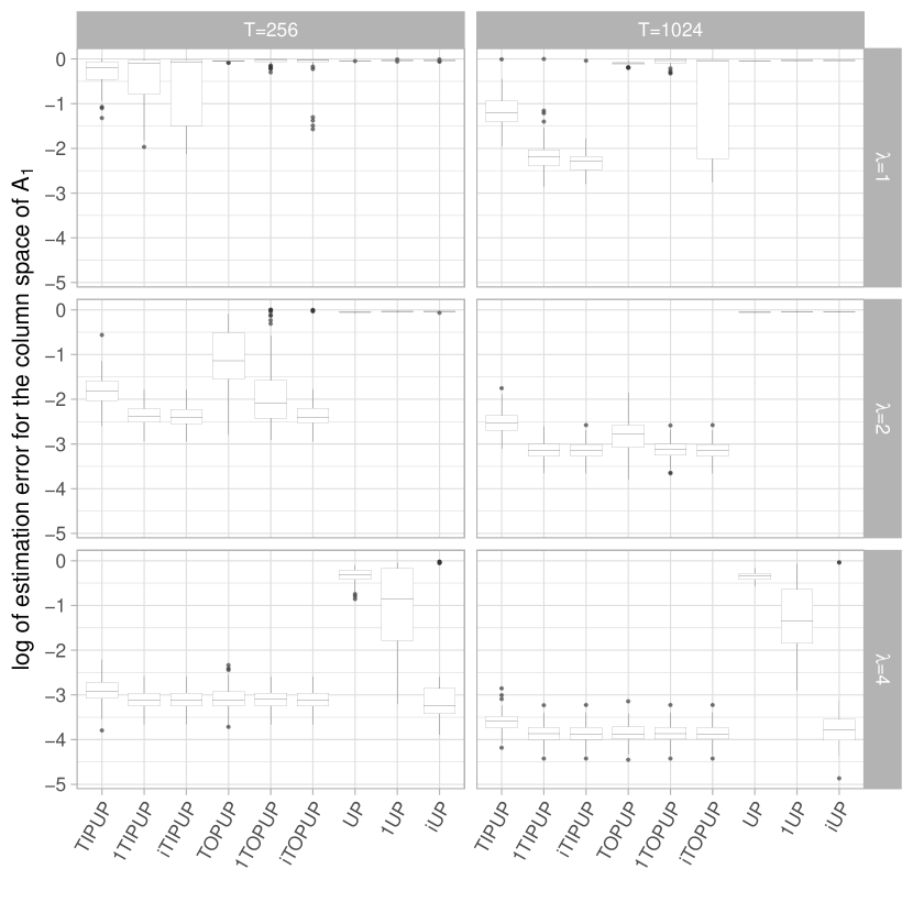
Figure 1: Experiment 1 under Configuration I. Boxplot of the logarithm of the estimation error of $A_{1}$. Nine methods (i)-(ix) are considered in total. Three rows correspond to three signal-to-noise strengths $\lambda=1,2,4$. Two columns correspond to two sample sizes $T=256,1024$.

It is somewhat surprising to observe, from the top left panel in Figure 1 ($T=256$ and $\lambda=1$), that in the small sample size and low signal strength case, the median error of iTIPUP is larger than that of 1TIPUP, which in turn is larger than TIPUP, whereas the order is reversed under stronger signal to noise ratio or with larger sample size shown in the other panels. Furthermore, the top right panel in Figure 1 shows that, with weak signal to noise ratio, the TIPUP based methods perform better than the TOPUP based methods. This observation coincides with the results in Corollaries 3.1 and 3.2, which together state that iTOPUP requires larger signal-to-noise ratio for consistency than iTIPUP. Figure 2 produces some deeper insight, where the trajectories of the iterative methods (including initial estimations, estimations after one iteration, and the estimations after final convergence) of the 100 repetitions are connected, for the $T=256$ case. The top two panels show that when signal is weak and the sample size is small, the initial estimates may be poor, and the iterative methods may need certain accuracy in the initial estimates to produce further improvement. This reemphasizes the condition on the initial estimate in the theorems. The bottom two panels show that when signal is stronger, the relatively more accurate initial estimates enable the iterative methods to improve the estimates. Again, TOPUP initial estimates are not as accurate as the TIPUP estimates.

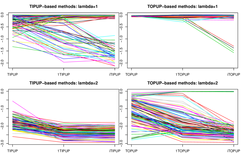
Figure 2: Experiment 1 under Configuration I. Trajectory of the logarithm of the estimation error of $A_{1}$ with fixed sample size $T=256$. Two rows correspond to two signal-to-noise strengths $\lambda=1,2$. Two columns correspond to TIPUP-based and TOPUP-based methods respectively.

Experiment 2 under Configuration I. We use the same setting as above, but vary $h_{0}=1,2,\ldots,5$, and fix $\hat{r}_{2}=1$ in the process of the estimation. Figure 3 provides the results. It can be seen that when there is no signal cancellation, the choice of $h_{0}$ does not affect the performance dramatically. When $h_{0}$ increases, the performance of all TIPUP-based and TOPUP-based algorithms becomes slightly worse most of the time.

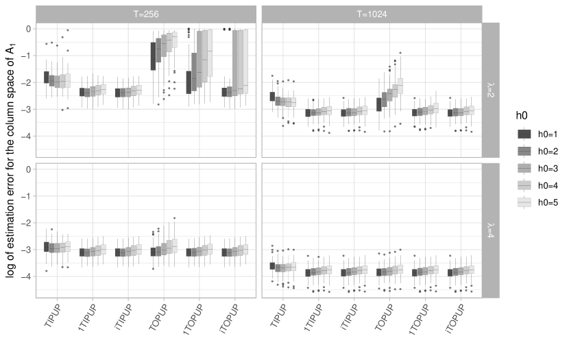
Figure 3: Experiment 2 under Configuration I. Boxplot of the logarithm of the estimation error of $A_{1}$. Six methods (iv)-(ix) with five choices of $h_{0}$ are considered in total. Two rows correspond to two signal-to-noise strengths $\lambda=2,4$. Two columns correspond to two sample sizes $T=256,1024$.

Experiment 3 under Configuration I. This experiment is conducted to verify the bounds on the sample size for iTOPUP in Corollary 3.3 and for iTIPUP in Corollary 3.4. We set the off-diagonal entries of the covariance matrices of the noise as $\psi_{1}=\psi_{2}=0.4$ and the AR coefficient of the factor time series as $\phi=0.9$, and vary the sample size $T=16,64,256,1024,4096$ and signal strength $\lambda=1,2,4,8$. Again, we use $h_{0}=1$ and $\hat{r}_{2}=1$ in the process of the estimation.

Table 1 provides the values of $\delta_{0},\delta_{1}$ in Assumption 3 as signal strength $\lambda$ varies and the lower bounds on the sample size in (3.25) and (3.27) when the values of $\delta_{0},\delta_{1}$ are plugged in. We have $\delta_{2}=0$ in this case and $d=d_{1}\times d_{2}=256$. Figure 4 shows the simulation results, where the raw estimation error instead of the logarithm is given. When the raw errors are close to 1, it implies the estimation is not accurate. It is corroborated that the sample size $T$ can be much smaller than $d$ in the strong factor case.

$\lambda$	$\delta_{0}$	$\delta_{1}$	iTOPUP bound (3.25)	iTIPUP bound (3.27)
1	1.00	1.00	4096.00	256.00
2	1.00	1.00	4096.00	256.00
4	0.82	0.86	829.44	81.00
8	0.57	0.61	51.84	5.06

Table 1: Experiment 3 under Configuration I. This table provides the values of $\delta_{0},\delta_{1}$ in Assumption 3 as signal strength $\lambda$ varies and the lower bounds on the sample size in (3.25) and (3.27) when the values of $\delta_{0},\delta_{1}$ are plugged in.

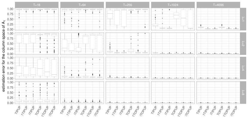
Figure 4: Experiment 3 under Configuration I. Boxplot of the estimation error of $A_{1}$. Six methods (iv)-(ix) are considered in total. Four rows correspond to four signal-to-noise strengths $\lambda=1,2,4,8$. Five columns correspond to five sample sizes $T=16,64,256,1024,4096$. This figure corroborates the theoretical lower bounds on the sample size in (3.25) and (3.27).

Under Configuration II, we performed two experiments: the two AR coefficients for the two independent univariate time series $f_{1t}$ and $f_{2t}$ are $\phi_{1}=0.8$ and $\phi_{2}=0.6$ in Experiment 1 and $\phi_{1}=0.8$ and $\phi_{2}=-0.8$ in Experiment 2. Experiment 1 under configuration II satisfies Assumption 2(i)-(ii) because there is no signal cancellation; Experiment 2 under configuration II satisfies Assumption 2(i) for TOPUP related methods. When $h_{0}=1$, Experiment 2 does not satisfy Assumption 2(ii) for TIPUP related methods as there is a severe signal cancellation. However, using $h_{0}=2$ significantly reduces signal cancellation as lag 2 auto-cross-covariance does not cancel each other in TIPUP related methods.

Experiment 1 under Configuration II. Figure 5 shows the boxplot of the logarithm of the estimation errors of 8 methods including (iv)-(ix) and mixed (x)-(xi) with TIPUP initiation and TOPUP iteration. Again, the performance of the mixed (xii)-(xiii) procedures with iTIPUP iteration is not as good as that of iTIPUP hence not shown. Here we use different sample sizes, with the signal strength fixed at $\lambda=1$ and two $h_{0}$ values: $h_{0}=1$ and $h_{0}=2$. The theoretical $\lambda_{1}$ defined in (3.5) and $\lambda_{1}^{*}$ in (3.6) under the stationary auto-cross-moments of the factor process are given in the figure. Note that they are different for different $h_{0}$. It shows that the mixed TIPUP-1TOPUP method can slightly improve 1TOPUP because of the better initialization. With larger sample size $T=1024$, TIPUP-1TOPUP also slightly outperforms 1TIPUP. In this case, using the larger $h_{0}=2$ provides slightly poorer performance than $h_{0}=1$, as the lag-2 autocorrelation is significantly smaller than that of lag 1 for the underlying AR(1) process with $\phi_{2}=0.6$. The extra term adds limited signal, shown by the small differences in $\lambda_{1}$ and $\lambda_{1}^{*}$, but incorporates extra noise terms in the estimators. To see more clearly the impact of $h_{0}$, we show the boxplots of the estimated $\lambda_{1}^{*}$ and $\lambda_{1}$ using iTIPUP and iTOPUP, respectively, for $h_{0}=1,2$ and $3$, under different sample sizes in Figure 6. The theoretical values are marked with a diamond. It is seen that the estimated values are relatively close to the theoretical values. More importantly, they decrease as $h_{0}$ increases in this no-signal cancellation case.

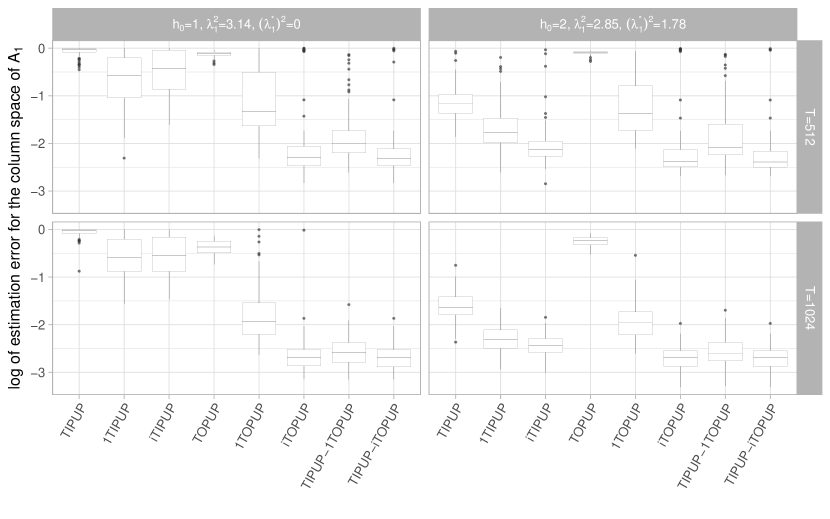
Figure 5: Experiment 1 under Configuration II. Boxplot of the logarithm of the estimation error of $A_{1}$. Eight methods are considered in total. Two rows correspond to two sample sizes $T=512,1024$. Two columns correspond to two choices of $h_{0}$. The population signal strengths $\lambda_{1}^{2}$ (3.5) and $\lambda_{1}^{*2}$ (3.6) for different $h_{0}$ are provided on the top.

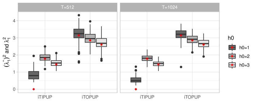
Figure 6: Experiment 1 under Configuration II. Boxplot of the sample estimates of the signal strengths $\lambda_{1}^{2}$ (3.5) and $\lambda_{1}^{*2}$ (3.6) over 100 replications for iTIPUP and iTOPUP with three choices of $h_{0}$. Two panels correspond to two sample sizes $T=512,1024$. The superimposed red diamonds are the population version of the signal strengths.

Experiment 2 under Configuration II. When $\phi_{1}=0.8$ and $\phi_{2}=-0.8$, we can readily check that $\mathbb{E}(F_{t}F_{t-1}^{\top})=(\phi_{1}+\phi_{2})\sigma^{2}=0$. Therefore, in the TIPUP-related procedure for estimating $A_{1}$ with $h_{0}=1$, the signal completely cancels out. Since the ranks $r_{1}$ and $r_{2}$ are fixed, we have $\delta_{2}=\infty$ for $h_{0}=1$, and the corresponding $\lambda_{1}^{*}=0$. Figure 7 shows the boxplot of the logarithm of the estimation error of $A_{1}$ for 8 methods including (iv)-(ix) and mixed (x)-(xi) with two choices of $h_{0}=1$ and $h_{0}=2$. We fix the signal strength to be $\lambda=1$ to isolate the effect of $h_{0}$. When $h_{0}=1$, both initialization TIPUP and TOPUP do not perform well. But 1TOPUP and iTOPUP improve the performance of TOPUP significantly with TOPUP iteration while 1TIPUP and iTIPUP cannot improve TIPUP. This is because signal cancellation has significant impact on TIPUP based procedures while having no impact on TOPUP based procedures. To our pleasant surprise, when $h_{0}=1$, the mixed TIPUP-1TOPUP is better than both 1TIPUP and 1TOPUP, and the mixed TIPUP-iTOPUP is similar to iTOPUP and much better than iTIPUP. When using $h_{0}=2$, the noise cancellation is mild and $(\lambda_{1}^{*})^{2}=1.78$. Since $r_{k}$ are fixed, we have $\delta_{2}<\infty$. Note that in this case the signal using TIPUP only comes from lag-2 cross product and is weaker than that using TOPUP related procedures. The difference does not have impact on the convergence rate, but on the signal to noise ratio. Comparing the left two subfigures with the right ones of Figure 7, it is seen that using $h_{0}=2$ always boosts the performance of TIPUP-related methods significantly. Meanwhile, the TOPUP based methods are not sensitive to the choice of $h_{0}$. When $h_{0}=2$, the non-iterative TIPUP performs better than TOPUP, 1TIPUP performs better than 1TOPUP, but after convergence, iTOPUP performs better than iTIPUP. Because the initialization TIPUP is better than TOPUP for $h_{0}=2$, it is of no surprise to see that TIPUP-1TOPUP behaves better than 1TIPUP and 1TOPUP, and TIPUP-iTOPUP is similar as iTOPUP and slightly better than iTIPUP.

Figure 7: Experiment 2 under Configuration II. Boxplot of the logarithm of the estimation error of $A_{1}$. 8 methods are considered in total. Two rows correspond to two sample sizes $T=512,1024$. Two columns correspond to two choices of $h_{0}$. The population signal strengths $\lambda_{1}^{2}$ (3.5) and $\lambda_{1}^{*2}$ (3.6) for different $h_{0}$ are provided on the top.

Again, to see more clearly the impact of $h_{0}$ in this case with noise cancellation, we show the boxplots of the estimated $\lambda_{1}^{*}$ and $\lambda_{1}$ using iTIPUP and iTOPUP, respectively, for $h_{0}=1,2$ and $3$ in Figure 8. It is seen that the iTOPUP procedure remains robust in estimating $\lambda_{1}$ under the noise-cancellation case. And $\lambda_{1}$ decreases as $h_{0}$ increases. However, iTIPUP is very different. Although when using $h_{0}=1$ the estimated $\lambda_{1}^{*}$ significantly overestimates the theoretical value $\lambda_{1}^{*}=0$, they are still much less than those from using $h_{0}=2$ and $3$. The reversed order of the magnitude of $\lambda_{1}^{*}$ as $h_{0}$ increases can be potentially used to detect signal cancellation in practice, though the theoretical property of the estimators of $\lambda_{1}^{*}$ (e.g. standard deviation) is technically challenging to obtain. In practice, when one observes such a reversed order, it is recommended to use iTOPUP as a conservative estimator. Of course, the behaviors of $\lambda_{k}$ and $\lambda_{k}^{*}$ depend on the auto-cross-moment structure of the underlying factor process. For example, if the factor process follows a MA(2) model with zero lag-1 autocorrelation ($f_{t}=e_{t}+\theta_{2}e_{t-2}$), then $\lambda_{1}$ and $\lambda_{1}^{*}$ under $h_{0}=2$ would be larger than those under both $h_{0}=1$ and $h_{0}=3$. But we expect that the pattern of $\lambda_{1}$ under different $h_{0}$ would be similar to that of $\lambda_{1}^{*}$ under different $h_{0}$, if there is no severe signal cancellation. Severe signal cancellation would make the patterns different.

Figure 8: Experiment 2 under Configuration II. Boxplot of the sample estimates of the signal strengths $\lambda_{1}^{2}$ (3.5) and $\lambda_{1}^{*2}$ (3.6) over 100 replications for iTIPUP and iTOPUP with three choices of $h_{0}$. Two panels correspond to two sample sizes $T=512,1024$. The superimposed red diamonds are the population version of the signal strengths.

Experiment under Configuration III. With order-3 tensor factor model (A.2), Configuration III satisfies Assumption 2, and Figure 9 shows the results. The message is almost the same as in Figure 3 for the matrix factor model. That is, TIPUP offers better initialization than TOPUP, which supports the theoretically smaller requirement on the sample size by TIPUP; iterative methods are better than one-step methods, which are in turn better than the non-iterative methods; when there is no signal cancellation, the iterative methods are in general not sensitive to the choice of $h_{0}$ and the non-iterative and one-step methods tend to behave slightly worse with larger values of $h_{0}$; when iTOPUP converges, its performance is better than that of iTIPUP as shown in the bottom right panel, which also verifies the theoretical claim of faster convergence rate of iTOPUP.

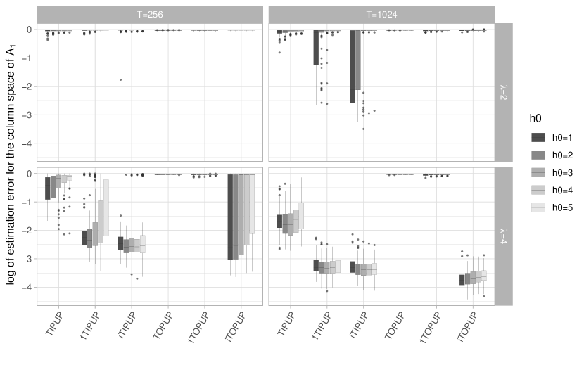
Figure 9: Experiment under Configuration III for order-3 tensor factor model. Boxplot of the logarithm of the estimation error of $A_{1}$. Six methods (iv)-(ix) with five choices of $h_{0}$ are considered in total. Two rows correspond to two signal-to-noise strengths $\lambda=2,4$. Two columns correspond to two sample sizes $T=256,1024$.

Appendix B Proof of Theorem 3.2

We focus on the case of $K=2$ as the iTIPUP begins with mode-$k$ matrix unfolding. In particular, we sometimes give explicit expressions only in the case of $k=1$ and $K=2$. For $K=2$, we observe a matrix time series with $X_{t}=A_{1}F_{t}A_{2}^{\top}+E_{t}\in\mathbb{R}^{d_{1}\times d_{2}}$. Recall that under the conditional expectation $\overline{\mathbb{E}}$, $F_{1},...F_{T}$ are fixed. Let $U_{1}$, $U_{2}$ be the left singular matrices of $A_{1}$ and $A_{2}$ respectively with $r_{k}=$rank$(U_{k})=$rank$(A_{k})$.

We outline the proof as follows. Let $L^{(m)}_{k}$ be the loss (2.1) for $\widehat{U}_{k}^{(m)}$ or equivalently the spectral norm error for $\widehat{P}_{k}^{(m)}=\widehat{U}_{k}^{(m)}\widehat{U}_{k}^{(m)\top}$, $k=1,...,K$, and $L^{(m)}$ their maximum,

$$L^{(m)}_{k}=\|\widehat{P}_{k}^{(m)}-P_{k}\|_{\rm S},\quad L^{(m)}=\max_{k=1,2,...,K}L^{(m)}_{k}.$$ (B.1)

From Chen, Yang and Zhang (2021), $\overline{\mathbb{E}}\big{[}L^{(0)}_{k}\big{]}\lesssim{R}^{*(0)}_{k}$ as we mentioned in (3.14). By applying the Gaussian concentration inequality for Lipschitz functions and Lemme G.2 in their analysis, we have

$$L^{(0)}\leq C_{1}^{(\text{\tiny TIPUP})}R^{*(0)}\ \text{ with }\ {R}^{*(0)}=\max_{1\leq k\leq K}{R}^{*(0)}_{k}$$ (B.2)

in an event $\Omega_{0}$ with $\overline{\mathbb{P}}(\Omega_{0})\geq 1-5^{-1}\sum_{k=1}^{K}e^{-d_{k}}$. This is similar to (B.10) below.

After the initialization with $\widehat{U}_{k}^{(0)}$, the algorithm iteratively produces estimates $\widehat{U}_{k}^{(m)}$ from $m=1$ to $m=J$. Define the matrix-valued operator $\text{TIPUP}_{1}(\cdot)$ as

$$\text{TIPUP}_{1}(\widetilde{U}_{2})=\bigg{(}\sum_{t=h+1}^{T}\frac{X_{t-h}\widetilde{U}_{2}\widetilde{U}_{2}^{\top}X_{t}^{\top}}{T-h},h=1,...,h_{0}\bigg{)}\in\mathbb{R}^{d_{1}\times(d_{1}h_{0})}$$

for any matrix-valued variable $\widetilde{U}_{2}\in\mathbb{R}^{d_{2}\times r_{2}}$. Given $\widehat{U}_{2}^{(m)}$, the $(m+1)$-th iteration produces estimates

$$\widehat{U}_{1}^{(m+1)}=\text{LSVD}_{r_{1}}\big{(}\text{TIPUP}_{1}(\widehat{U}_{2}^{(m)})\big{)},\quad\widehat{P}_{1}^{(m+1)}=\widehat{U}_{1}^{(m+1)}\widehat{U}_{1}^{(m+1)\top}.$$

The “noiseless” version of this update is given by

$$\Theta_{1,h}^{*}(\widetilde{U}_{2})=\sum_{t=h+1}^{T}\frac{A_{1}F_{t-h}A_{2}^{\top}\widetilde{U}_{2}\widetilde{U}_{2}^{\top}A_{2}F_{t}^{\top}A_{1}^{\top}}{T-h},\quad\overline{\mathbb{E}}[\text{TIPUP}_{1}](\widetilde{U}_{2})=\Theta_{1,1:h_{0}}^{*}(\widetilde{U}_{2}),$$ (B.3)

with $\Theta_{1,1:h_{0}}^{*}(\widetilde{U}_{2})=\big{(}\Theta_{1,h}^{*}(\widetilde{U}_{2}),h=1,...,h_{0}\big{)}$ as in (3.4), giving error free “estimates”,

$$U_{1}=\text{LSVD}_{r_{1}}\big{(}\overline{\mathbb{E}}[\text{TIPUP}_{1}](\widehat{U}_{2}^{(m)})\big{)},\quad P_{1}=U_{1}U_{1}^{\top},$$

when $\overline{\mathbb{E}}[\text{TIPUP}_{1}](\widehat{U}_{2}^{(m)})$ is of rank $r_{1}$. Thus, by Wedin’s theorem (Wedin (1972)),

$$L_{1}^{(m+1)}=\big{\|}\widehat{P}_{1}^{(m+1)}-P_{1}\big{\|}_{\rm S}\leq\frac{2\|\text{TIPUP}_{1}(\widehat{U}_{2}^{(m)})-\overline{\mathbb{E}}[\text{TIPUP}_{1}](\widehat{U}_{2}^{(m)})\|_{\rm S}}{\sigma_{r_{1}}(\overline{\mathbb{E}}[\text{TIPUP}_{1}](\widehat{U}_{2}^{(m)}))}.$$

We note that $\widehat{U}_{2}^{(m)}$ is plugged-in after the conditional expectation in $\overline{\mathbb{E}}[\text{TIPUP}_{1}](\cdot)$. For general $1\leq k\leq K$, we define $\text{TIPUP}_{k}(\widetilde{U}_{-k})$ and $\overline{\mathbb{E}}[\text{TIPUP}_{k}](\widetilde{U}_{-k})$ as matrix-valued functions of $\widetilde{U}_{-k}=\odot_{j\neq k}\widetilde{U}_{j}$. We will prove by induction that $\sigma_{r_{k}}(\overline{\mathbb{E}}[\text{TIPUP}_{k}](\widehat{U}_{-k}^{(m)}))$, the denominator in the above inequality, is no smaller than a half of its ideal version as in (3.6), e.g.

$$2\sigma_{r_{1}}(\overline{\mathbb{E}}[\text{TIPUP}_{1}](\widehat{U}_{2}^{(m)}))\geq\sigma_{r_{1}}(\overline{\mathbb{E}}[\text{TIPUP}_{1}](U_{2}))=h_{0}^{1/2}{\lambda}_{1}^{*2},$$ (B.4)

in the case of $k=1$ and $K=2$. It would then follow that

$$L_{1}^{(m+1)}=\big{\|}\widehat{P}_{1}^{(m+1)}-P_{1}\big{\|}_{\rm S}\leq\frac{\|\text{TIPUP}_{1}(\widehat{U}_{2}^{(m)})-\overline{\mathbb{E}}[\text{TIPUP}_{1}](\widehat{U}_{2}^{(m)})\|_{\rm S}}{h_{0}^{1/2}{\lambda}_{1}^{*2}/4}.$$ (B.5)

To bound the numerator on the right-hand side of (B.5), we write

$$\text{TIPUP}_{1}(\widetilde{U}_{2})-\overline{\mathbb{E}}[\text{TIPUP}_{1}](\widetilde{U}_{2})=\sum_{j=1}^{3}\Big{(}\Delta^{*}_{j,1,h}\big{(}\widetilde{U}_{2}\widetilde{U}_{2}^{\top}\big{)},h=1,\ldots,h_{0}\Big{)}\in\mathbb{R}^{d_{1}\times(d_{1}h_{0})}$$ (B.6)

as both $\text{TIPUP}_{1}(\widetilde{U}_{2})$ and $\overline{\mathbb{E}}[\text{TIPUP}_{1}](\widetilde{U}_{2})$ are linear in $\widetilde{U}_{2}\widetilde{U}_{2}^{\top}$, where for any $\widetilde{M}_{2}\in\mathbb{R}^{d_{2}\times d_{2}}$

$$\Delta_{1}^{*}(\widetilde{M}_{2}):=\Delta_{1,1,h}^{*}(\widetilde{M}_{2}):=\hbox{$\sum_{t=h+1}^{T}$}A_{1}F_{t-h}A_{2}^{\top}\widetilde{M}_{2}E_{t}^{\top}/(T-h),$$

$$\Delta_{2}^{*}(\widetilde{M}_{2}):=\Delta_{2,1,h}^{*}(\widetilde{M}_{2}):=\hbox{$\sum_{t=h+1}^{T}$}E_{t-h}\widetilde{M}_{2}A_{2}F_{t}^{\top}A_{1}^{\top}/(T-h),$$

$$\Delta_{3}^{*}(\widetilde{M}_{2}):=\Delta_{3,1,h}^{*}(\widetilde{M}_{2}):=\hbox{$\sum_{t=h+1}^{T}$}E_{t-h}\widetilde{M}_{2}E_{t}^{\top}/(T-h).$$

As $\Delta_{j,1,h}^{*}(\widetilde{M}_{2})$ is linear in $\widetilde{M}_{2}$, the numerator on the right-hand of (B.5) can be bounded by

$$\|\text{TIPUP}_{1}(\widehat{U}_{2}^{(m)})-\overline{\mathbb{E}}[\text{TIPUP}_{1}](\widehat{U}_{2}^{(m)})\|_{\rm S}$$ (B.7)

$$\leq \|\text{TIPUP}_{1}(U_{2})-\overline{\mathbb{E}}[\text{TIPUP}_{1}](U_{2})\|_{\rm S}+L^{(m)}(2K-2)\sum_{j=1}^{3}h_{0}^{1/2}\max_{h\leq h_{0}}\|\Delta_{j,1,h}^{*}\|_{1,S,S}$$

with an application of Cauchy-Schwarz inequality for the sum over $h=1,\ldots,h_{0}$, where $\|\Delta_{j,1,h}^{*}\|_{1,S,S}$ are norms of the $\mathbb{R}^{d_{2}\times d_{2}}\to\mathbb{R}^{d_{1}\times d_{1}}$ linear mappings $\Delta_{j,1,h}^{*}$ defined as

$$\|\Delta_{j}^{*}\|_{1,S,S}=\|\Delta_{j,1,h}^{*}\|_{1,S,S}:=\max_{\|\widetilde{M}_{2}\|_{\rm S}\leq 1,\text{rank}(\widetilde{M}_{2})\leq r_{2}}\big{\|}\Delta_{j,1,h}^{*}(\widetilde{M}_{2})\big{\|}_{\rm S}.$$

For general $1\leq k\leq K$, $\Delta_{j,k,h}^{*}$ is an $\mathbb{R}^{d_{-k}\times d_{-k}}$ to $\mathbb{R}^{d_{k}\times d_{k}}$ mapping, and (G.2) of Lemma G.1 (iii) gives the general version of (B.7) with

$$\big{\|}\Delta_{j,k,h}^{*}\big{\|}_{k,S,S}:=\max_{\|\widetilde{M}_{\ell}\|_{\rm S}\leq 1,\text{rank}(\widetilde{M}_{\ell})\leq r_{\ell},\forall\ell\neq k}\big{\|}\Delta_{j,k,h}^{*}\big{(}\odot_{\ell\neq k}\widetilde{M}_{\ell}\big{)}\big{\|}_{\rm S}$$

because it is applied to $\widetilde{M}_{-k}=\odot_{\ell\neq k}\widehat{P}_{\ell}^{(m)}-\odot_{\ell\neq k}P_{\ell}$ with $\|\widehat{P}_{\ell}^{(m)}-P_{\ell}\|_{\rm S}\leq L^{(m)}$.

We claim that in certain events $\Omega_{j},j=1,2,3$, with $\overline{\mathbb{P}}(\Omega_{j})\geq 1-5^{-1}\sum_{k=1}^{K}e^{-d_{k}}$,

$$\big{\|}\Delta_{j,k,h}^{*}\big{\|}_{k,S,S}\leq\rho{\lambda}_{k}^{*2}\big{/}\big{(}24(K-1)\big{)},\quad\forall 1\leq k\leq K.$$ (B.8)

For simplicity, we will only prove this inequality for $k=1$ and $K=2$ in the form of

$$\overline{\mathbb{P}}\left\{\|\Delta_{j}^{*}\|_{1,S,S}=\max_{\|\widetilde{M}_{2}\|_{\rm S}\leq 1,\text{rank}(\widetilde{M}_{2})\leq r_{2}}\big{\|}\Delta_{j,1,h}^{*}(\widetilde{M}_{2})\big{\|}_{\rm S}\geq\rho{\lambda}_{1}^{*2}\big{/}24\right\}\leq 5^{-1}e^{-d_{2}}$$ (B.9)

as the proof of its counter part for general $1\leq k\leq K$ is similar.

Define the ideal version of the ratio in (B.5) for general $1\leq k\leq K$ as

$$L^{(\text{\footnotesize ideal})}_{k}=\frac{\|\text{TIPUP}_{k}(U_{-k})-\overline{\mathbb{E}}[\text{TIPUP}_{k}](U_{-k})\|_{\rm S}}{h_{0}^{1/2}\lambda_{k}^{*2}/4},\quad L^{(\text{\footnotesize ideal})}=\max_{1\leq k\leq K}L^{(\text{\footnotesize ideal})}_{k}.$$

As $U_{-k}=\odot_{j\neq k}U_{j}$ is true and deterministic, by (3.15) and (B.6), the proof of (B.8) also implies

$$L^{(\text{\footnotesize ideal})}\leq C_{1}^{(\text{\tiny TIPUP})}R^{*(\text{\footnotesize ideal})}\ \text{ with }\ {R}^{*(\text{\footnotesize ideal})}=\max_{1\leq k\leq K}{R}^{*(\text{\footnotesize ideal})}_{k}$$ (B.10)

in an event $\Omega_{4}$ with $\overline{\mathbb{P}}(\Omega_{4})\leq 5^{-1}\sum_{k=1}^{K}e^{-d_{k}}$, where $R^{*(\text{\footnotesize ideal})}_{k}$ is as in (3.15).

Putting together (B.1), (B.5), (B.7) and (B.8), we find that in the event $\cap_{j=0}^{4}\Omega_{j}$

$$L^{(m+1)}_{k}\leq L^{(\text{\footnotesize ideal})}_{k}+L^{(m)}\frac{(6K-6)\max_{j,k,h}\big{\|}\Delta_{j,k,h}^{*}\big{\|}_{k,S,S}}{{\lambda}_{k}^{*2}/4}\leq L^{(\text{\footnotesize ideal})}_{k}+\rho L^{(m)},$$ (B.11)

which implies by induction

$$L^{(m+1)}\leq(1+\cdots+\rho^{m})L^{(\text{\footnotesize ideal})}+\rho^{m+1}L^{(0)},$$ (B.12)

and then the conclusions follows from (B.2) and (B.10). We divide the rest of the proof into 4 steps to prove (B.9) for $j=1,2,3$ and (B.4).

Step 1. We prove (B.9) for the $\Delta_{1}^{*}(\widetilde{M}_{2})$ in (B.6). By Lemma G.1 (ii), there exist $\widetilde{M}^{(\ell,\ell^{\prime})}\in\mathbb{R}^{d_{2}\times d_{2}}$ of the form $W_{\ell}Q_{\ell^{\prime}}^{\top}$ with $W_{\ell}\in\mathbb{R}^{d_{2}\times r_{2}}$, $Q_{\ell^{\prime}}\in\mathbb{R}^{d_{2}\times r_{2}}$, $1\leq\ell,\ell^{\prime}\leq N_{d_{2}r_{2},1/8}:=17^{d_{2}r_{2}}$, such that $\|\widetilde{M}^{(\ell,\ell^{\prime})}\|_{\rm S}\leq 1$, rank$(\widetilde{M}^{(\ell,\ell^{\prime})})\leq r_{2}$ and

$$\|\Delta_{1}^{*}\|_{1,S,S}=\|\Delta_{1,1,h}^{*}\|_{1,S,S}\leq 2\max_{\ell,\ell^{\prime}\leq N_{d_{2}r_{2},1/8}}\left\|\sum_{t=h+1}^{T}\frac{A_{1}F_{t-h}A_{2}^{\top}\widetilde{M}^{(\ell,\ell^{\prime})}E_{t}^{\top}}{T-h}\right\|_{\rm S}.$$

To bound $\|\Delta_{1,k,h}^{*}\|_{1,S,S}$ for general $k\leq K$, we just need to replace $\widetilde{M}^{(\ell,\ell^{\prime})}$ by $\odot_{j\neq k}\widetilde{M}_{j}^{(\ell,\ell^{\prime})}$ and $N_{d_{2}r_{2},1/8}$ by $N_{d^{*}_{-k},1/(8K-8)}$ with $d^{*}_{-k}=\sum_{j\neq k}d_{j}r_{j}$ as in Lemma G.1 (iii). We apply the Gaussian concentration inequality to the right-hand side above. Elementary calculation shows that

$$\left|\left\|\sum_{t=h+1}^{T}A_{1}F_{t-h}A_{2}^{\top}\widetilde{M}^{(\ell,\ell^{\prime})}E_{t}^{\top}\right\|_{\rm S}-\left\|\sum_{t=h+1}^{T}A_{1}F_{t-h}A_{2}^{\top}\widetilde{M}^{(\ell,\ell^{\prime})}E_{t}^{*\top}\right\|_{\rm S}\right|$$

$$\leq \left\|(A_{1}F_{1}A_{2}^{\top},...,A_{1}F_{T-h}A_{2}^{\top})\begin{pmatrix}\widetilde{M}^{(\ell,\ell^{\prime})}(E_{h+1}^{\top}-E_{h+1}^{*\top})\\ \vdots\\ \widetilde{M}^{(\ell,\ell^{\prime})}(E_{T}^{\top}-E_{T}^{*\top})\end{pmatrix}\right\|_{\rm S}$$

$$\leq \left\|(A_{1}F_{1}A_{2}^{\top},...,A_{1}F_{T-h}A_{2}^{\top})\right\|_{\rm S}^{1/2}\left\|\text{diag}\Big{(}\widetilde{M}^{(\ell,\ell^{\prime})}\Big{)}\begin{pmatrix}E_{h+1}^{\top}-E_{h+1}^{*\top}\\ \vdots\\ E_{T}^{\top}-E_{T}^{*\top}\end{pmatrix}\right\|_{\rm S}$$

$$\leq \sqrt{T}\|\Theta_{1,0}^{*}\|_{\rm S}^{1/2}\left\|\begin{pmatrix}E_{h+1}^{\top}-E_{h+1}^{*\top}\\ \vdots\\ E_{T}^{\top}-E_{T}^{*\top}\end{pmatrix}\right\|_{\rm F}.$$

That is, $\left\|\sum_{t=h+1}^{T}A_{1}F_{t-h}A_{2}^{\top}\widetilde{M}^{(\ell,\ell^{\prime})}E_{t}^{\top}\right\|_{\rm S}$ is a $\sqrt{T}\|\Theta_{1,0}^{*}\|_{\rm S}^{1/2}$ Lipschitz function of $(E_{1},\ldots,E_{T})$. Employing similar arguments in the proof of Theorem 2 in Chen, Yang and Zhang (2021), we have

$$\bar{\mathbb{E}}\left\|\sum_{t=h+1}^{T}\frac{A_{1}F_{t-h}A_{2}^{\top}\widetilde{M}^{(\ell,\ell^{\prime})}E_{t}^{\top}}{T-h}\right\|_{\rm S}\leq\frac{\sigma(8Td_{1})^{1/2}}{T-h}\|\Theta_{1,0}^{*}\|_{\rm S}^{1/2}.$$

Then, by Gaussian concentration inequalities for Lipschitz functions,

$$\mathbb{P}\left(\left\|\sum_{t=h+1}^{T}\frac{A_{1}F_{t-h}A_{2}^{\top}\widetilde{M}^{(\ell,\ell^{\prime})}E_{t}^{\top}}{T-h}\right\|_{\rm S}-\frac{\sigma(8Td_{1})^{1/2}}{T-h}\|\Theta_{1,0}^{*}\|_{\rm S}^{1/2}\geq\frac{\sigma\sqrt{T}}{T-h}\|\Theta_{1,0}^{*}\|_{\rm S}^{1/2}x\right)\leq e^{-\frac{x^{2}}{2}}.$$

Hence,

$$\mathbb{P}\left(\|\Delta_{1}^{*}\|_{1,S,S}/2\geq\frac{\sigma(8Td_{1})^{1/2}}{T-h}\|\Theta_{1,0}^{*}\|_{\rm S}^{1/2}+\frac{\sigma\sqrt{T}}{T-h}\|\Theta_{1,0}^{*}\|_{\rm S}^{1/2}x\right)\leq N_{d_{2}r_{2},1/8}^{2}e^{-\frac{x^{2}}{2}}.$$

As $T\geq 4h_{0}$ and $K=2$, this implies with $x\asymp\sqrt{d_{2}r_{2}}$ that in an event with at least probability $1-e^{-d_{2}}/5$,

$$\|\Delta_{1}^{*}\|_{1,S,S}\leq\frac{C_{1,K}^{(\text{\footnotesize iter})}\sigma T^{-1/2}\|\Theta_{1,0}^{*}\|_{\rm S}^{1/2}(\sqrt{d_{1}}+\sqrt{d_{2}r_{2}})}{24(K-1)}\leq\frac{C_{1,K}^{(\text{\footnotesize iter})}(1+\sqrt{d_{2}r_{2}/d_{1}})\lambda_{1}^{*2}R_{1}^{*(\text{\footnotesize ideal})}}{24},$$

with the ${R}_{k}^{*(\text{\footnotesize ideal})}$ in (3.15) and a constant $C_{1,K}^{(\text{\footnotesize iter})}$ depending on $K$ only. In this event, (3.17) gives $24({\lambda}^{*}_{k})^{-2}\|\Delta_{1,k,h}^{*}\|_{k,S,S}\leq C_{1,K}^{(\text{\footnotesize iter})}({R}_{k}^{*(\text{\footnotesize ideal})}+R_{k}^{*(\text{\footnotesize add})})\leq\rho$. Thus, (B.9) holds for $\Delta_{1}^{*}(\widetilde{M}_{2})$.

Step 2. Inequality (B.9) for $\Delta_{2}^{*}(\widetilde{M}_{2})$ follow from the same argument as the above step.

Step 3. Here we prove (B.9) for the $\Delta_{3}^{*}(\widetilde{M}_{2})$ in (B.6). By Lemma G.1 (ii), we can find $U_{2}^{(\ell)},U_{2}^{(\ell^{\prime})}\in\mathbb{R}^{d_{2}\times r_{2}}$, $1\leq\ell,\ell^{\prime}\leq N_{d_{2}r_{2},1/8}$ such that $\|U_{2}^{(\ell)}\|_{\rm S}\leq 1$, $\|U_{2}^{(\ell^{\prime})}\|_{\rm S}\leq 1$ and

$$\|\Delta_{3}^{*}\|_{1,S,S}=\|\Delta_{3,1,h}^{*}\|_{1,S,S}\leq 2\max_{1\leq\ell,\ell^{\prime}\leq N_{d_{2}r_{2},1/8}}\left\|\sum_{t=h+1}^{T}\frac{E_{t-h}U_{2}^{(\ell)}U_{2}^{(\ell^{\prime})\top}E_{t}^{\top}}{T-h}\right\|_{\rm S}.$$ (B.13)

We split the sum into two terms over the index sets, $S_{1}=\{(h,2h]\cup(3h,4h]\cup\cdots\}\cap(h,T]$ and its complement $S_{2}$ in $(h,T]$, so that $\{E_{t-h},t\in S_{a}\}$ is independent of $\{E_{t},t\in S_{a}\}$ for each $a=1,2$. Let $n_{a}=|S_{a}|r_{2}$. Define $G_{a}=(E_{t-h}U_{2}^{(\ell)},t\in S_{a})\in\mathbb{R}^{d_{1}\times n_{a}}$ and $H_{a}=(E_{t}U_{2}^{(\ell^{\prime})},t\in S_{a})\in\mathbb{R}^{d_{1}\times n_{a}}$. Then, $G_{a}$, $H_{a}$ are two independent Gaussian matrices. Note that

$$\left\|\sum_{t\in S_{a}}\frac{E_{t-h}U_{2}^{(\ell)}U_{2}^{(\ell^{\prime})\top}E_{t}^{\top}}{T-h}\right\|_{\rm S}=\left\|\frac{G_{a}H_{a}^{\top}}{T-h}\right\|_{\rm S}.$$ (B.14)

Moreover, by Assumption 1, $\textsf{Var}(u^{\top}\text{vec}(G_{a}))\leq\sigma^{2}$ and $\textsf{Var}(u^{\top}\text{vec}(H_{a}))\leq\sigma^{2}$ for all unit vectors $u\in\mathbb{R}^{d_{1}n_{a}}$, so that by Lemme G.2 (i),

$$\mathbb{P}\Big{\{}\|G_{a}H_{a}^{\top}\|_{\rm S}/\sigma^{2}\geq d_{1}+2\sqrt{d_{1}n_{a}}+x(x+2\sqrt{n_{a}}+2\sqrt{d_{1}})\Big{\}}\leq e^{-x^{2}/2},\quad x>0.$$

As $\sum_{a=1}^{2}n_{a}=r_{2}(T-h)$, it follows from (B.13), (B.14) and the above inequality that

$$\mathbb{P}\left\{\frac{\|\Delta_{3,1,h}^{*}\|_{1,S,S}}{4\sigma^{2}}\geq\frac{(\sqrt{d_{1}}+x)^{2}}{T-h}+\frac{\sqrt{2r_{2}}(\sqrt{d_{1}}+x)}{\sqrt{T-h}}\right\}\leq 2N_{d_{2}r_{2},1/8}^{2}e^{-x^{2}/2}.$$

Thus, with $h_{0}\leq T/4$, $x\asymp\sqrt{d_{1}}+\sqrt{d^{*}_{-1}}$ and some constant $C_{1,K}^{(\text{\footnotesize iter})}$ depending on $K$ only,

$$\|\Delta_{3,1,h}^{*}\|_{1,S,S}\leq\frac{(C_{1,K}^{(\text{\footnotesize iter})}-1)(1-h_{0}/T)^{2}\sigma^{2}}{24(K-1)}\bigg{(}\frac{(\sqrt{d_{1}}+\sqrt{d^{*}_{-1}})\sqrt{r_{-1}}}{(T-h_{0})^{1/2}}+\frac{(\sqrt{d_{1}}+\sqrt{d^{*}_{-1}})^{2}}{T-h_{0}}\bigg{)}$$ (B.15)

with at least probability $1-e^{-d_{1}}/5$. As ${\lambda}_{k}^{*}\leq\|\Theta_{1,0}^{*}\|_{\rm S}^{1/2}/(1-h_{0}/T)^{1/2}$ by (3.6) and (3.3),

$${R}_{1}^{*(\text{\footnotesize ideal})}\geq({\lambda}_{1}^{*})^{-1}(1-h_{0}/T)\sigma(T-h_{0})^{-1/2}\sqrt{d_{1}}+({\lambda}_{1}^{*})^{-2}\sigma T^{-1/2}\sigma\sqrt{d_{1}r_{-1}}$$

by (3.15). Thus, in the event (B.15) and for $k=1$ and $K=2$,

$$\|\Delta_{3,1,h}^{*}\|_{1,S,S}$$

$$\leq \frac{C_{1,K}^{(\text{\footnotesize iter})}-1}{24}\bigg{(}\Big{(}1+\sqrt{d^{*}_{-1}/d_{1}}\Big{)}{\lambda}_{1}^{*2}{R}_{1}^{*(\text{\footnotesize ideal})}+\Big{(}1+\sqrt{d^{*}_{-1}/d_{1}}\Big{)}^{2}{\lambda}_{1}^{*2}\big{(}{R}_{1}^{*(\text{\footnotesize ideal})}\big{)}^{2}\bigg{)}$$

$$\leq ({\lambda}_{1}^{*2}/24)(C_{1,K}^{(\text{\footnotesize iter})}-1)(1+{R}_{k}^{*(\text{\footnotesize ideal})}+R_{k}^{*(\text{\footnotesize add})})({R}_{k}^{*(\text{\footnotesize ideal})}+R_{k}^{*(\text{\footnotesize add})})$$

which is no greater than ${\lambda}_{1}^{*2}\rho/24$ by the condition (3.17). This yields (B.9) for $\Delta_{3}^{*}(\widetilde{M}_{2})$.

Step 4. Next, we prove (B.4) in the event $\cap_{j=0}^{4}\Omega_{j}$. Note that,

$$\|\Theta_{1,h}^{*}(\widehat{U}_{2}^{(m)})-\Theta_{1,h}^{*}(U_{2})\|_{\rm S}=\left\|\sum_{t=h+1}^{T}\frac{A_{1}F_{t-h}A_{2}^{\top}(\widehat{U}_{2}^{(m)}\widehat{U}_{2}^{(m)\top}-U_{2}U_{2}^{\top})A_{2}F_{t}^{\top}A_{1}^{\top}}{T-h}\right\|_{\rm S}$$

$$=\frac{1}{T-h}\left\|(A_{1}F_{1}A_{2}^{\top},...,A_{1}F_{T-h}A_{2}^{\top})\begin{pmatrix}(\widehat{U}_{2}^{(m)}\widehat{U}_{2}^{(m)\top}-U_{2}U_{2}^{\top})A_{2}F_{1}^{\top}A_{1}^{\top}\\ \vdots\\ (\widehat{U}_{2}^{(m)}\widehat{U}_{2}^{(m)\top}-U_{2}U_{2}^{\top})A_{2}F_{T-h}^{\top}A_{1}^{\top}\end{pmatrix}\right\|_{\rm S}$$

$$\leq\frac{1}{T-h}\left\|(A_{1}F_{1}A_{2}^{\top},...,A_{1}F_{T-h}A_{2}^{\top})\right\|_{\rm S}\left\|\text{diag}\Big{(}\widehat{U}_{2}^{(m)}\widehat{U}_{2}^{(m)\top}-U_{2}U_{2}^{\top}\Big{)}\begin{pmatrix}A_{2}F_{1}^{\top}A_{1}^{\top}\\ \vdots\\ A_{2}F_{T-h}^{\top}A_{1}^{\top}\end{pmatrix}\right\|_{\rm S}$$

$$\leq\|\widehat{U}_{2}^{(m)}\widehat{U}_{2}^{(m)\top}-U_{2}U_{2}^{\top}\|_{\rm S}\|\Theta_{1,0}^{*}\|_{\rm S}/(1-h/T)$$

$$\leq L^{(m)}\|\Theta_{1,0}^{*}\|_{\rm S}/(1-h_{0}/T).$$

Hence, by the Cauchy-Schwarz inequality and (B.3),

$$\|\overline{\mathbb{E}}[\text{TIPUP}_{1}](\widehat{U}_{2}^{(m)})-\overline{\mathbb{E}}[\text{TIPUP}_{1}](U_{2})\|_{\rm S}\leq\sqrt{h_{0}}L^{(m)}\|\Theta_{1,0}^{*}\|_{\rm S}/(1-h_{0}/T).$$

By (3.6), ${\lambda}_{1}^{*2}h_{0}^{1/2}=\sigma_{r_{1}}\big{(}\operatorname*{\text{mat}_{1}}1(\Theta_{1,1:h_{0}}^{*})\big{)}=\sigma_{r_{1}}\big{(}\overline{\mathbb{E}}[\text{TIPUP}_{1}](U_{2})\big{)}$. Thus, by Weyl’s inequality,

$$\sigma_{r_{1}}(\overline{\mathbb{E}}[\text{TIPUP}_{1}](\widehat{U}_{2}^{(m)}))\geq{\lambda}_{1}^{*2}h_{0}^{1/2}-2\sqrt{h_{0}}L^{(m)}\|\Theta_{1,0}^{*}\|_{\rm S}\geq\sigma_{r_{1}}(\overline{\mathbb{E}}[\text{TIPUP}_{1}](U_{2}))\big{/}2={\lambda}_{1}^{*2}h_{0}^{1/2}/2.$$

when $\min_{k\leq K}{\lambda}_{k}^{*2}\geq 4L^{(m)}\|\Theta_{1,0}^{*}\|_{\rm S}$. We prove this condition by induction in the event $\cap_{j=0}^{4}\Omega_{j}$. By (3.17) and (B.2), $4L^{(0)}\|\Theta_{1,0}^{*}\|_{\rm S}\leq 4C_{1}^{(\text{\tiny TIPUP})}R^{*(0)}\|\Theta_{1,0}^{*}\|_{\rm S}\leq\min_{k\leq K}{\lambda}_{k}^{*2}$. Given the induction assumption $4L^{(m)}\|\Theta_{1,0}^{*}\|_{\rm S}\leq\min_{k\leq K}{\lambda}_{k}^{*2}$, (B.4) holds for the same $m$, so that (B.12), (B.10) and (B.2),

$$L^{(m+1)}\leq C_{1}^{(\text{\tiny TIPUP})}\big{\{}2(1+\cdots+\rho^{m})R^{*(\text{\footnotesize ideal})}+\rho^{m+1}R^{*(0)}\big{\}}\leq C_{1}^{(\text{\tiny TIPUP})}2(1-\rho)^{-1}R^{*(0)}.$$

It then follows from (3.17) that $4L^{(m+1)}\|\Theta_{1,0}^{*}\|_{\rm S}\leq C_{1}^{(\text{\tiny TIPUP})}8(1-\rho)^{-1}R^{*(0)}\|\Theta_{1,0}^{*}\|_{\rm S}\leq\min_{k\leq K}{\lambda}_{k}^{*2}$. This completes the induction and the proof of the entire theorem.

Appendix C Proof of Theorem 3.1

Again, we focus on the case of $K=2$ as the iTOPUP also begins with mode-$k$ matrix unfolding. In particular, we sometimes give explicit expressions only in the case of $k=1$ and $K=2$. For $K=2$, we observe a matrix time series with $X_{t}=A_{1}F_{t}A_{2}^{\top}+E_{t}\in\mathbb{R}^{d_{1}\times d_{2}}$. Recall $\overline{\mathbb{E}}(\cdot)=\mathbb{E}(\cdot|\{{\cal F}_{1},...,{\cal F}_{T}\})$. Let $U_{1}$, $U_{2}$ be the left singular matrices of $A_{1}$ and $A_{2}$ respectively with $r_{k}=$rank$(U_{k})=$rank$(A_{k})$. Recall $\odot$ is kronecker product and $\otimes$ is tensor product.

We outline the proof as follows, which has exactly the same structure as the proofs of Theorem 3.2.

Let $L^{(m)}_{k}=\|\widehat{P}_{k}^{(m)}-P_{k}\|_{\rm S}$ and $L^{(m)}=\max_{k\leq K}L^{(m)}_{k}$ as in (B.1). From Chen, Yang and Zhang (2021), $\overline{\mathbb{E}}\big{[}L^{(0)}_{k}\big{]}\lesssim{R}^{(0)}_{k}$ as we mentioned in (3.7). By applying the Gaussian concentration inequality for Lipschitz functions and Lemme G.2 in their analysis, we have

$$L^{(0)}\leq C_{1}^{(\text{\tiny TOPUP})}R^{(0)}\ \text{ with }\ {R}^{(0)}=\max_{1\leq k\leq K}{R}^{(0)}_{k}$$ (C.1)

in an event $\Omega_{0}$ with $\overline{\mathbb{P}}(\Omega_{0})\geq 1-5^{-1}\sum_{k=1}^{K}e^{-d_{k}}$. This is similar to (C.8) below.

For any matrices ${\widetilde{U}}_{j}\in\mathbb{R}^{d_{j}\times r_{j}}$ with $r_{K+j}=r_{j}$, define

$${\rm{TOPUP}}_{k}({\widetilde{U}}_{j},1\leq j\leq 2K,j\neq k,j\neq K+K)$$

$$= \left({\rm{mat}}_{k}\Big{(}\widehat{\Sigma}_{h}\times_{j=1}^{k-1}{\widetilde{U}}_{j}\times_{j=k+1}^{K+k-1}{\widetilde{U}}_{j}\times_{j=K+k+1}^{2K}{\widetilde{U}}_{j}\Big{)}\ h=1,...,h_{0}\right)$$ (C.2)

and its noiseless version $\overline{\mathbb{E}}[{\rm{TOPUP}}_{k}]$. Here both ${\rm{TOPUP}}_{k}$ and $\overline{\mathbb{E}}[{\rm{TOPUP}}_{k}]$ are viewed as $\mathbb{R}^{d_{k}\times(d_{k}r_{-k}^{2}h_{0})}$-valued $(2K-2)$-linear mappings with input ${\widetilde{U}}_{j}$. When ${\widetilde{U}}_{K+j}={\widetilde{U}}_{j}$ for all $j\neq k$, we write (C) as ${\rm{TOPUP}}_{k}({\widetilde{U}}_{-k})$ and its noiseless version $\overline{\mathbb{E}}[{\rm{TOPUP}}_{k}]({\widetilde{U}}_{-k})$. After the initialization with $\widehat{U}_{k}^{(0)}$, the algorithm iteratively produces estimates $\widehat{U}_{k}^{(m+1)}$ as the rank-$r_{k}$ left singular matrix of ${\rm{TOPUP}}_{k}\big{(}\widehat{U}_{1:(k-1)}^{(m+1)},\widehat{U}_{(k+1):K}^{(m)}\big{)}$. For $K=2$ and $k=1$,

$$\text{TOPUP}_{1}(\widetilde{U}_{2},\widetilde{U}_{4})=\text{mat}_{1}\bigg{(}\sum_{t=h+1}^{T}\frac{X_{t-h}\widetilde{U}_{2}\otimes X_{t}\widetilde{U}_{4}}{T-h},h=1,\ldots,h_{0}\bigg{)}\in\mathbb{R}^{d_{1}\times(d_{1}r_{2}^{2}h_{0})}.$$

for any $\widetilde{U}_{j}\in\mathbb{R}^{d_{2}\times r_{2}},j=2,4$. Given $\widehat{U}_{2}^{(m)}$, the $(m+1)$-th iteration produces estimates

$$\widehat{U}_{1}^{(m+1)}=\text{LSVD}_{r_{1}}\big{(}\text{TOPUP}_{1}\big{(}\widehat{U}_{2}^{(m)}\big{)}\big{)},\quad\widehat{P}_{1}^{(m+1)}=\widehat{U}_{1}^{(m+1)}\widehat{U}_{1}^{(m+1)\top}.$$

When $\text{rank}\big{(}\overline{\mathbb{E}}[\text{TOPUP}_{1}](\widehat{U}_{2}^{(m)})\big{)}=r_{1}$, the “noiseless” version of this update is error free,

$$U_{1}=\text{LSVD}_{r_{1}}\big{(}\overline{\mathbb{E}}[\text{TOPUP}_{1}](\widehat{U}_{2}^{(m)})\big{)},\quad P_{1}=U_{1}U_{1}^{\top}.$$

Thus, by Wedin’s theorem, (Wedin (1972)),

$$L_{1}^{(m+1)}=\big{\|}\widehat{P}_{1}^{(m+1)}-P_{1}\big{\|}_{\rm S}\leq\frac{2\|\text{TOPUP}_{1}(\widehat{U}_{2}^{(m)})-\overline{\mathbb{E}}[\text{TOPUP}_{1}](\widehat{U}_{2}^{(m)})\|_{\rm S}}{\sigma_{r_{1}}(\overline{\mathbb{E}}[\text{TOPUP}_{1}](\widehat{U}_{2}^{(m)}))}.$$

We will prove by induction that $\sigma_{r_{k}}\big{(}\overline{\mathbb{E}}[\text{TOPUP}_{k}]\big{(}\widehat{U}_{1:(k-1)}^{(m)},\widehat{U}_{(k+1):K}^{(m-1)}\big{)}\big{)}$, the general version of the denominator on the right-hand side above, is no smaller than a half of its ideal version as in (3.5), e.g.

$$2\sigma_{r_{1}}(\overline{\mathbb{E}}[\text{TOPUP}_{1}](\widehat{U}_{2}^{(m)}))\geq\sigma_{r_{1}}(\overline{\mathbb{E}}[\text{TOPUP}_{1}](U_{2}))=h_{0}^{1/2}{\lambda}_{1}^{2},$$ (C.3)

in the case of $k=1$ and $K=2$. It would then follow that

$$L_{1}^{(m+1)}=\big{\|}\widehat{P}_{1}^{(m+1)}-P_{1}\big{\|}_{\rm S}\leq\frac{\|\text{TOPUP}_{1}(\widehat{U}_{2}^{(m)})-\overline{\mathbb{E}}[\text{TOPUP}_{1}](\widehat{U}_{2}^{(m)})\|_{\rm S}}{h_{0}^{1/2}{\lambda}_{1}^{2}/4}.$$ (C.4)

To bound the numerator on the right-hand side of (C.4), we write

$$\Delta\big{(}\widetilde{U}_{2},\widetilde{U}_{4}\big{)}=\text{TOPUP}_{1}\big{(}\widetilde{U}_{2},\widetilde{U}_{4}\big{)}-\overline{\mathbb{E}}\big{[}\text{TOPUP}_{1}\big{]}\big{(}\widetilde{U}_{2},\widetilde{U}_{4}\big{)}$$

and notice that for any orthonormal matrices $Q_{j}\in\mathbb{R}^{d_{2}\times r_{2}}$

$$\big{\|}\Delta\big{(}Q_{2}Q_{2}^{\top}\widetilde{U}_{2},Q_{4}Q_{4}^{\top}\widetilde{U}_{4}\big{)}\big{\|}_{\rm S}\leq\big{\|}\Delta\big{(}Q_{2},Q_{4}\big{)}\big{\|}_{\rm S}\|Q_{2}^{\top}\widetilde{U}_{2}\|_{\rm S}\|Q_{4}^{\top}\widetilde{U}_{4}\|_{\rm S}$$

as the outer product is taken in (C). Moreover, because $\Delta\big{(}\widetilde{U}_{2},\widetilde{U}_{4}\big{)}$ is bilinear,

$$\big{\|}\Delta\big{(}\widetilde{U}_{2},\widetilde{U}_{2}\big{)}\big{\|}_{\rm S} \leq\big{\|}\Delta\big{(}P_{2}\widetilde{U}_{2},P_{2}\widetilde{U}_{2}\big{)}\big{\|}_{\rm S}+\big{\|}\Delta\big{(}P_{2}\widetilde{U}_{2},P_{2}^{\perp}\widetilde{U}_{2}\big{)}\big{\|}_{\rm S}+\big{\|}\Delta\big{(}P_{2}^{\perp}\widetilde{U}_{2},\widetilde{U}_{2}\big{)}\big{\|}_{\rm S}$$

$$\leq\big{\|}\Delta\big{(}U_{2},U_{2}\big{)}\big{\|}_{\rm S}+\big{\|}\Delta\big{(}U_{2},Q_{2}\big{)}\big{\|}_{\rm S}\|P_{2}^{\perp}\widetilde{U}_{2}\|_{\rm S}+\big{\|}\Delta\big{(}Q_{2},\widetilde{U}_{2}\big{)}\big{\|}_{\rm S}\|P_{2}^{\perp}\widetilde{U}_{2}\|_{\rm S},$$

where $Q_{2}=$LSVD${}_{r_{k}}(P_{2}^{\perp}\widetilde{U}_{2})$ and $P_{2}^{\perp}=I_{d_{2}}-P_{2}$. Thus, due to $\|P_{2}^{\perp}\widehat{U}_{2}^{(m)}\|_{\rm S}\leq\|P_{2}-\widehat{P}_{2}^{(m)}\|_{\rm S}\leq L^{(m)}$, the numerator on the right-hand of (C.4) can be bounded by

$$\|\text{TOPUP}_{1}(\widehat{U}_{2}^{(m)})-\overline{\mathbb{E}}[\text{TOPUP}_{1}](\widehat{U}_{2}^{(m)})\|_{\rm S}$$ (C.5)

$$\leq \|\text{TOPUP}_{1}(U_{2})-\overline{\mathbb{E}}[\text{TOPUP}_{1}](U_{2})\|_{\rm S}+L^{(m)}(2K-2)\sum_{j=1}^{3}h_{0}^{1/2}\max_{h\leq h_{0}}\|\Delta_{j,1,h}\|_{1,S,S},$$

where $\|\Delta\|_{1,S,S}:=\max_{\|\widetilde{U}_{j}\|_{\rm S}\leq 1,\text{rank}(\widetilde{U}_{j})=r_{2},j=2,4}\big{\|}\Delta(\widetilde{U}_{2},\widetilde{U}_{4})\big{\|}_{\rm S}$ for any bilinear $\Delta$ and

$$\Delta_{1}\big{(}\widetilde{U}_{2},\widetilde{U}_{4}\big{)}:=\Delta_{1,1,h}\big{(}\widetilde{U}_{2},\widetilde{U}_{4}\big{)} :=\frac{1}{T-h}\sum_{t=h+1}^{T}\operatorname*{\text{mat}_{1}}1(A_{1}F_{t-h}A_{2}^{\top}\widetilde{U}_{2}\otimes E_{t}\widetilde{U}_{4}),$$

$$\Delta_{2}\big{(}\widetilde{U}_{2},\widetilde{U}_{4}\big{)}:=\Delta_{2,1,h}\big{(}\widetilde{U}_{2},\widetilde{U}_{4}\big{)} :=\frac{1}{T-h}\sum_{t=h+1}^{T}\operatorname*{\text{mat}_{1}}1(E_{t-h}\widetilde{U}_{2}\otimes A_{1}F_{t}^{\top}A_{2}^{\top}\widetilde{U}_{4}),$$

$$\Delta_{3}\big{(}\widetilde{U}_{2},\widetilde{U}_{4}\big{)}:=\Delta_{3,1,h}\big{(}\widetilde{U}_{2},\widetilde{U}_{4}\big{)} :=\frac{1}{T-h}\sum_{t=h+1}^{T}\operatorname*{\text{mat}_{1}}1(E_{t-h}\widetilde{U}_{2}\otimes E_{t}\widetilde{U}_{4}).$$

We claim that in certain events $\Omega_{j},j=1,2,3$, with $\overline{\mathbb{P}}(\Omega_{j})\geq 1-5^{-1}\sum_{k=1}^{K}e^{-d_{k}}$, $\rho<1$,

$$\big{\|}\Delta_{j,k,h}\big{\|}_{k,S,S}\leq\rho{\lambda}_{k}^{2}\big{/}\big{(}24(K-1)\big{)},\quad\forall 1\leq k\leq K,$$ (C.6)

in (C.5). For simplicity, we will only prove this inequality for $k=1$ and $K=2$,

$$\overline{\mathbb{P}}\left\{\|\Delta_{j}\|_{1,S,S}=\max_{\|\widetilde{M}_{2}\|_{\rm S}\leq 1}\big{\|}\Delta_{j,1,h}\big{(}\widetilde{U}_{2},\widetilde{U}_{4}\big{)}\big{\|}_{\rm S}\geq\rho{\lambda}_{1}^{2}\big{/}24\right\}\leq 5^{-1}e^{-d_{2}}.$$ (C.7)

Define the ideal version of the ratio in (C.4) for general $1\leq k\leq K$ as

$$L^{(\text{\footnotesize ideal})}_{k} =\frac{4\|\text{TOPUP}_{k}(U_{-k})-\overline{\mathbb{E}}[\text{TOPUP}_{k}](U_{-k})\|_{\rm S}}{\sigma_{r_{k}}(\overline{\mathbb{E}}[\text{TOPUP}_{k}](U_{-k}))},$$

$$L^{(\text{\footnotesize ideal})} =\max_{1\leq k\leq K}L^{(\text{\footnotesize ideal})}_{k}.$$

Note that $\sigma_{r_{k}}(\overline{\mathbb{E}}[\text{TOPUP}_{k}](U_{-k}))=h_{0}^{1/2}\lambda_{k}^{2}$. By (3.8), the proof of (C.6) also implies

$$L^{(\text{\footnotesize ideal})}\leq C_{1}^{(\text{\tiny TOPUP})}R^{(\text{\footnotesize ideal})}\ \text{ with }\ {R}^{(\text{\footnotesize ideal})}=\max_{1\leq k\leq K}{R}^{(\text{\footnotesize ideal})}_{k}$$ (C.8)

in an event $\Omega_{4}$ with $\overline{\mathbb{P}}(\Omega_{4})\leq 5^{-1}\sum_{k=1}^{K}e^{-d_{k}}$, where $R^{(\text{\footnotesize ideal})}_{k}$ is as in (3.8).

It follows from (B.1), (C.4), (C.5) and (C.6) that in the event $\bigcap_{j=0}^{4}\Omega_{j}$

$$L^{(m+1)}_{k}\leq L^{(\text{\footnotesize ideal})}_{k}+24(K-1)L^{(m)}\max_{j,k,h}\big{\|}\Delta_{j,k,h}\big{\|}_{k,S,S}\big{/}{\lambda}_{k}^{2}\leq L^{(\text{\footnotesize ideal})}_{k}+\rho L^{(m)},$$ (C.9)

which implies by induction

$$L^{(m+1)}\leq(1+\cdots+\rho^{m})L^{(\text{\footnotesize ideal})}+\rho^{m+1}L^{(0)},$$ (C.10)

and then the conclusions follows from (C.1) and (C.8). Again, we divide the rest of the proof into 4 steps to prove (C.7) for $j=1,2,3$ and (C.3).

Step 1. We prove (C.7) for the $\Delta_{1}\big{(}\widetilde{U}_{2},\widetilde{U}_{4}\big{)}$. By Lemma G.1 (ii), there exist $U_{2}^{(\ell)},U_{2}^{(\ell^{\prime})}\in\mathbb{R}^{d_{2}\times r_{2}}$, $1\leq\ell,\ell^{\prime}\leq N_{d_{2}r_{2},1/8}:=17^{d_{2}r_{2}}$, such that $\|U_{2}^{(\ell)}\|_{\rm S}\leq 1$, $\|U_{2}^{(\ell^{\prime})}\|_{\rm S}\leq 1$ and

$$\|\Delta_{1}\|_{1,S,S}=\|\Delta_{1,1,h}\|_{1,S,S}\leq 2\max_{\ell,\ell^{\prime}\leq N_{d_{2}r_{2},1/8}}\left\|\sum_{t=h+1}^{T}\frac{\operatorname*{\text{mat}_{1}}1(A_{1}F_{t-h}A_{2}^{\top}U_{2}^{(\ell)}\otimes E_{t}U_{2}^{(\ell^{\prime})})}{T-h}\right\|_{\rm S}.$$

We apply the Gaussian concentration inequality to the right-hand side above. Elementary calculation shows that

$$\left|\left\|\sum_{t=h+1}^{T}\operatorname*{\text{mat}_{1}}1(A_{1}F_{t-h}A_{2}^{\top}U_{2}^{(\ell)}\otimes E_{t}U_{2}^{(\ell^{\prime})})\right\|_{\rm S}-\left\|\sum_{t=h+1}^{T}\operatorname*{\text{mat}_{1}}1(A_{1}F_{t-h}A_{2}^{\top}U_{2}^{(\ell)}\otimes E_{t}^{*}U_{2}^{(\ell^{\prime})})\right\|_{\rm S}\right|$$

$$\leq \left\|\sum_{t=h+1}^{T}\operatorname*{\text{mat}_{1}}1(A_{1}F_{t-h}A_{2}^{\top}U_{2}^{(\ell)}\otimes(E_{t}-E_{t}^{*})U_{2}^{(\ell^{\prime})})\right\|_{\rm S}$$

$$\leq \left\|(\operatorname*{\text{mat}_{1}}1(A_{1}F_{1}A_{2}^{\top}\otimes I_{d_{1}}),...,\operatorname*{\text{mat}_{1}}1(A_{1}F_{T-h}A_{2}^{\top}\otimes I_{d_{1}}))\begin{pmatrix}U_{2}^{(\ell)}\odot I_{d_{1}}\odot(E_{h+1}-E_{h+1}^{*})U_{2}^{(\ell^{\prime})}\\ \vdots\\ U_{2}^{(\ell)}\odot I_{d_{1}}\odot(E_{T}-E_{T}^{*})U_{2}^{(\ell^{\prime})}\end{pmatrix}\right\|_{\rm S}$$

$$\leq \sqrt{T}\|\Theta_{1,0}^{*}\|_{\rm S}^{1/2}\|U_{2}^{(\ell)}\|_{\rm S}\|U_{2}^{(\ell^{\prime})}\|_{\rm S}\left\|\begin{pmatrix}E_{h+1}-E_{h+1}^{*}\\ \vdots\\ E_{T}-E_{T}^{*}\end{pmatrix}\right\|_{\rm F}.$$

That is, $\left\|\sum_{t=h+1}^{T}\operatorname*{\text{mat}_{1}}1(A_{1}F_{t-h}A_{2}^{\top}U_{2}^{(\ell)}\otimes E_{t}U_{2}^{(\ell^{\prime})})\right\|_{\rm S}$ is a $\sqrt{T}\|\Theta_{1,0}^{*}\|_{\rm S}^{1/2}$ Lipschitz function in $(E_{1},...,E_{T})$. Employing similar arguments in the proof of Theorem 1 in Chen, Yang and Zhang (2021), we have

$$\overline{\mathbb{E}}\left\|\sum_{t=h+1}^{T}\frac{\operatorname*{\text{mat}_{1}}1(A_{1}F_{t-h}A_{2}^{\top}U_{2}^{(\ell)}\otimes E_{t}U_{2}^{(\ell^{\prime})})}{T-h}\right\|_{\rm S}\leq\frac{\sigma(2T)^{1/2}(\sqrt{d_{1}}+\sqrt{d_{1}r_{2}^{2}})}{T-h}\|\Theta_{1,0}^{*}\|_{\rm S}^{1/2}$$

Then, by Gaussian concentration inequalities for Lipschitz functions,

$$\mathbb{P}\left(\left\|\sum_{t=h+1}^{T}\frac{\operatorname*{\text{mat}_{1}}1(A_{1}F_{t-h}A_{2}^{\top}U_{2}^{(\ell)}\otimes E_{t}U_{2}^{(\ell^{\prime})})}{T-h}\right\|_{\rm S}-\frac{\sigma(2T)^{1/2}(\sqrt{d_{1}}+\sqrt{d_{1}r_{2}^{2}})}{T-h}\|\Theta_{1,0}^{*}\|_{\rm S}^{1/2}\geq\frac{\sigma\sqrt{T}}{T-h}\|\Theta_{1,0}^{*}\|_{\rm S}^{1/2}x\right)$$

$$\leq 2e^{-\frac{x^{2}}{2}}.$$

Hence,

$$\mathbb{P}\left(\|\Delta_{1}\|_{1,S,S}/2\geq\frac{\sigma(2T)^{1/2}(\sqrt{d_{1}}+\sqrt{d_{1}r_{2}^{2}})}{T-h}\|\Theta_{1,0}^{*}\|_{\rm S}^{1/2}+\frac{\sigma\sqrt{T}}{T-h}\|\Theta_{1,0}^{*}\|_{\rm S}^{1/2}x\right)$$

$$\leq 2N_{d_{2}r_{2},1/8}^{2}e^{-\frac{x^{2}}{2}}.$$

As $T\geq 4h_{0}$, this implies with $x\asymp\sqrt{d_{2}r_{2}}$ that in an event with at least probability $1-e^{-d_{2}}/5$,

$$\|\Delta_{1}\|_{1,S,S} \leq\frac{C_{1,K}^{(\text{\footnotesize iter})}\sigma T^{-1/2}\|\Theta_{1,0}^{*}\|_{\rm S}^{1/2}(\sqrt{d_{1}}r_{2}+\sqrt{d_{2}r_{2}})}{24(K-1)}$$

$$\leq\frac{C_{1,K}^{(\text{\footnotesize iter})}(\lambda_{1}^{2}R_{1}^{(\text{\footnotesize ideal})}+\sigma T^{-1/2}\|\Theta_{1,0}^{*}\|_{\rm S}^{1/2}\sqrt{d_{2}r_{2}})}{24}$$

with the ${R}_{k}^{(\text{\footnotesize ideal})}$ in (3.8) and a constant $C_{1,K}^{(\text{\footnotesize iter})}$ depending on $K$ only. In this event, (3.10) gives $36({\lambda}_{k})^{-2}\|\Delta_{1,k,h}\|_{k,S,S}\leq C_{1,K}^{(\text{\footnotesize iter})}({R}_{k}^{(\text{\footnotesize ideal})}+R_{k}^{(\text{\footnotesize add})})\leq\rho$. Thus, (C.7) holds for $\Delta_{1}^{*}(\widetilde{M}_{2})$.

Step 2. Note that

$$\|\Delta_{2}\|_{1,S,S}=\max_{\begin{subarray}{c}\widetilde{U}_{2}\in\mathbb{R}^{d_{2}\times r_{2}},\widecheck{U}_{2}\in\mathbb{R}^{d_{2}\times r_{2}},\\ \|\widetilde{U}_{2}\|_{\rm S}\leq 1,\|\widecheck{U}_{2}\|_{\rm S}\leq 1\end{subarray}}\left\|\sum_{t=h+1}^{T}\frac{\operatorname*{\text{mat}_{1}}1(E_{t-h}\widetilde{U}_{2}\otimes U_{1}^{\top}A_{1}F_{t}A_{2}^{\top}\widecheck{U}_{2})}{T-h}\right\|_{\rm S}.$$

Then, inequality (C.7) for $\Delta_{2}\big{(}\widetilde{U}_{2},\widetilde{U}_{4}\big{)}$ follow from the same argument as the above step.

Step 3. Now we prove (C.7) for the $\Delta_{3}\big{(}\widetilde{U}_{2},\widetilde{U}_{4}\big{)}$. We split the sum into two terms over the index sets, $S_{1}=\{(h,2h]\cup(3h,4h]\cup\cdots\}\cap(h,T]$ and its complement $S_{2}$ in $(h,T]$, so that $\{E_{t-h},t\in S_{a}\}$ is independent of $\{E_{t},t\in S_{a}\}$ for each $a=1,2$. Let $n_{a}=|S_{a}|$.

By Lemma G.1 (ii), we can find $U_{2}^{(\ell)},U_{2}^{(\ell^{\prime})}\in\mathbb{R}^{d_{2}\times r_{2}}$, $1\leq\ell,\ell^{\prime}\leq N_{d_{2}r_{2},1/8}$ such that $\|U_{2}^{(\ell)}\|_{\rm S}\leq 1$, $\|U_{2}^{(\ell^{\prime})}\|_{\rm S}\leq 1$. In this case,

$$\|\Delta_{3}\|_{1,S,S}=\|\Delta_{3,1,h}\|_{1,S,S}\leq 2\max_{1\leq\ell,\ell^{\prime}\leq N_{d_{2}r_{2},1/8}}\left\|\sum_{t=h+1}^{T}\frac{\operatorname*{\text{mat}_{1}}1(E_{t-h}U_{2}^{(\ell)}\otimes E_{t}U_{2}^{(\ell^{\prime})})}{T-h}\right\|_{\rm S}.$$ (C.11)

Define $G_{a}=(E_{t-h}U_{2}^{(\ell)},t\in S_{a})$ and $H_{a}=(E_{t}U_{2}^{(\ell^{\prime})},t\in S_{a})$. Then, $G_{a}$, $H_{a}$ are two independent Gaussian matrices. By Lemma G.2(ii), for any $x>0$,

$$\mathbb{P}\left(\left\|\sum_{t\in S_{a}}\operatorname*{\text{mat}_{1}}1(E_{t-h}U_{2}^{(\ell)}\otimes E_{t}U_{2}^{(\ell^{\prime})})\right\|_{\rm S}\geq d_{1}\sqrt{r_{2}}+2r_{2}\sqrt{d_{1}n_{a}}+x^{2}+\sqrt{n_{a}}x+3\sqrt{d_{1}r_{2}}x\right)$$

$$\leq 2e^{-x^{2}/2}.$$

As in the derivation of $\|\Delta_{3}^{*}\|_{1,S,S}$ in the proof of Theorem 3.2, we have, with $x\asymp\sqrt{d_{2}r_{2}}$ and some constant $C_{1,K}^{(\text{\footnotesize iter})}$ depending on $K$ only,

$$\mathbb{P}\left(\|\Delta_{3,1,h}\|_{1,S,S}\geq\frac{C_{1,K}^{(\text{\footnotesize iter})}\sigma^{2}}{24}\left(\frac{r_{2}\sqrt{d_{1}}+\sqrt{d_{2}r_{2}}}{T^{1/2}}+\frac{d_{1}\sqrt{r_{2}}+d_{2}r_{2}+r_{2}\sqrt{d_{1}d_{2}}}{T}\right)\right)\leq e^{-d_{2}}/5.$$

This yields (C.7) for $\Delta_{3}\big{(}\widetilde{U}_{2},\widetilde{U}_{4}\big{)}$ as in the end of Step 1 for $\Delta_{1}\big{(}\widetilde{U}_{2},\widetilde{U}_{4}\big{)}$.

Step 4. Next, we consider the $r_{1}$-th largest singular value of $\sigma_{r_{1}}(\overline{\mathbb{E}}[\text{TOPUP}_{1}](\widehat{U}_{2}^{(m)}))$ in the event $\cap_{j=0}^{4}\Omega_{j}$. By definition, the left singular subspace of $\overline{\mathbb{E}}[\text{TOPUP}_{1}](\widehat{U}_{2}^{(m)})$ is $U_{1}$. Then,

$$\sigma_{r_{1}}(\overline{\mathbb{E}}[\text{TOPUP}_{1}](\widehat{U}_{2}^{(m)}))$$

$$= \sigma_{r_{1}}\left(\operatorname*{\text{mat}_{1}}1\left(\sum_{t=h+1}^{T}\frac{A_{1}F_{t-h}A_{2}^{\top}\widehat{U}_{2}^{(m)}\otimes A_{1}F_{t}A_{2}^{\top}\widehat{U}_{2}^{(m)}}{T-h},h=1,...,h_{0}\right)\right)$$

$$= \sigma_{r_{1}}\left(\operatorname*{\text{mat}_{1}}1\left(\sum_{t=h+1}^{T}\frac{A_{1}F_{t-h}A_{2}^{\top}U_{2}U_{2}^{\top}\widehat{U}_{2}^{(m)}\otimes A_{1}F_{t}A_{2}^{\top}U_{2}U_{2}^{\top}\widehat{U}_{2}^{(m)}}{T-h},h=1,...,h_{0}\right)\right)$$

$$= \sigma_{r_{1}}\left(\operatorname*{\text{mat}_{1}}1\left(\sum_{t=h+1}^{T}\frac{A_{1}F_{t-h}A_{2}^{\top}U_{2}\otimes A_{1}F_{t}A_{2}^{\top}U_{2}}{T-h},h=1,...,h_{0}\right)\cdot\left(U_{2}^{\top}\widehat{U}_{2}^{(m)}\odot I_{d_{1}}\odot U_{2}^{\top}\widehat{U}_{2}^{(m)}\odot I_{h_{0}}\right)\right)$$

$$\geq \sigma_{r_{1}}\left(\operatorname*{\text{mat}_{1}}1\left(\sum_{t=h+1}^{T}\frac{A_{1}F_{t-h}A_{2}^{\top}U_{2}\otimes A_{1}F_{t}A_{2}^{\top}U_{2}}{T-h},h=1,...,h_{0}\right)\right)\cdot\sigma_{\min}\left(U_{2}^{\top}\widehat{U}_{2}^{(m)}\odot I_{d_{1}}\odot U_{2}^{\top}\widehat{U}_{2}^{(m)}\odot I_{h_{0}}\right)$$

$$\geq \sigma_{r_{1}}\left(\operatorname*{\text{mat}_{1}}1\left(\sum_{t=h+1}^{T}\frac{A_{1}F_{t-h}A_{2}^{\top}\otimes A_{1}F_{t}A_{2}^{\top}}{T-h},h=1,...,h_{0}\right)\right)\cdot\sigma_{\min}\left(U_{2}^{\top}\widehat{U}_{2}^{(m)}\right)\cdot\sigma_{\min}\left(U_{2}^{\top}\widehat{U}_{2}^{(m)}\right)$$

$$\geq \sqrt{h_{0}}\lambda_{1}^{2}(1-L^{(m)2}).$$

The last step follows from the definitions in (2.1) and (B.1). If $L^{(m)}\leq 1/2$, then

$$\sigma_{r_{1}}(\overline{\mathbb{E}}[\text{TOPUP}_{1}](\widehat{U}_{2}^{(m)}))\geq\sqrt{h_{0}}\lambda_{1}^{2}/2.$$

By (3.5), ${\lambda}_{1}^{2}h_{0}^{1/2}=\sigma_{r_{1}}\big{(}{\text{mat}}_{1}(\Theta_{1,1:h_{0}})\big{)}=\sigma_{r_{1}}\big{(}{\text{mat}}_{1}(\overline{\mathbb{E}}[\text{TOPUP}_{1}](U_{2})\big{)}$. We prove this condition in the event $\cap_{j=0}^{4}\Omega_{j}$. By (3.10) and (C.1), $L^{(0)}\leq C_{1}^{(\text{\tiny TOPUP})}R^{(0)}\leq 1/2$. By induction, given $L^{(m)}\leq 1/2$, (C.3) holds for the same $m$. Applying (C.1), (C.8) and (C.10),

$$L^{(m+1)} \leq C_{1}^{(\text{\tiny TOPUP})}\big{\{}2(1+\cdots+\rho^{m})R^{(\text{\footnotesize ideal})}+\rho^{m+1}R^{(0)}\big{\}}\leq C_{1}^{(\text{\tiny TOPUP})}2(1-\rho)^{-1}R^{(0)}$$

$$\leq 1/2.$$

This completes the induction and the proof of the entire theorem.

Appendix D Proof of Theorem 3.4

Without loss of generality, we can assume $\sigma=1$. Within the probability space (3.33) ${\mathscr{P}}(T,d_{1},...,d_{K},\lambda)$, we study a specific model with $f_{2t}=f_{2t-1}$ for all $1\leq t\leq\lfloor T/2\rfloor$. Taking an average for each ${\cal X}_{2t}$ and ${\cal X}_{2t-1}$, $1\leq t\leq\lfloor T/2\rfloor$, we reduce by sufficiency the model to

$$\widetilde{\mathscr{P}}(\lfloor T/2\rfloor,d_{1},...,d_{K},\lambda)=\left\{{\cal X}_{1},...,{\cal X}_{\lfloor T/2\rfloor}:{\cal X}_{t}=\lambda\widetilde{f}_{t}\times_{1}a_{1}\times_{2}...\times_{K}a_{K}+\widetilde{\cal E}_{t},\text{ with }a_{k}\in\mathbb{R}^{d_{k}},\right.$$

$$\qquad\qquad\|a_{k}\|_{2}=1,1\leq k\leq K,\widetilde{f}_{t}\overset{i.i.d.}{\sim}N(0,1/2),\{\widetilde{f}_{t}\}_{t=1}^{\lfloor T/2\rfloor}\text{ independent of }\{\widetilde{\cal E}_{t}\}_{t=1}^{\lfloor T/2\rfloor},$$

$$\qquad\qquad\left.\widetilde{\cal E}_{t,j_{1},...,j_{K}}\overset{i.i.d.}{\sim}N(0,1/2)\text{ for all }1\leq t\leq\lfloor T/2\rfloor,1\leq j_{k}\leq d_{k},1\leq k\leq K\right\}.$$

For notation convenience, in the following of this section, we study the probability space

$$\widetilde{\mathscr{P}}(T,d_{1},...,d_{K},\lambda)=\left\{{\cal X}_{1},...,{\cal X}_{T}:{\cal X}_{t}=\lambda f_{t}\times_{1}a_{1}\times_{2}...\times_{K}a_{K}+{\cal E}_{t},\text{ with }a_{k}\in\mathbb{R}^{d_{k}},\right.$$ (D.1)

$$\qquad\qquad\|a_{k}\|_{2}=1,1\leq k\leq K,f_{t}\overset{i.i.d.}{\sim}N(0,1),\{f_{t}\}_{t=1}^{T}\text{ independent of }\{{\cal E}_{t}\}_{t=1}^{T},$$

$$\qquad\qquad\left.{\cal E}_{t,j_{1},...,j_{K}}\overset{i.i.d.}{\sim}N(0,1)\text{ for all }1\leq t\leq T,1\leq j_{k}\leq d_{k},1\leq k\leq K\right\}.$$

We first introduce some additional notation. For any probability distributions $\mathbb{P}$ and $\mathbb{Q}$, define total variation distance as $\mathsf{TV}(\mathbb{P},\mathbb{Q})=\sup_{B}|\mathbb{P}(B)-\mathbb{Q}(B)|$. We also write $\mathsf{TV}(p,q)$ if $p,q$ are the densities of $\mathbb{P}$ and $\mathbb{Q}$, respectively. Define

$$\tau_{N}=\frac{\kappa}{N},\qquad\eta_{N}=\frac{\kappa}{(K+2)^{4}N(\log N)^{2}},$$

where $\kappa$ is the size of the clique. For any $\mu\in\mathbb{R}$, denote $\phi_{\mu}$ as the density function of the $N(\mu,1)$ distribution, and let

$$\widebar{\phi}_{\mu}=\frac{1}{2}(\phi_{\mu}+\phi_{-\mu})$$

be the density function of the Gaussian mixture $\frac{1}{2}N(\mu,1)+\frac{1}{2}N(-\mu,1)$. We also define $\widetilde{\Xi}_{0}$ as a truncated normal distribution by the $N(0,1)$ distribution restricted on the interval $[-(K+2)\sqrt{\log N},(K+2)\sqrt{\log N}]$. For any $|\mu|\leq(K+2)\sqrt{\eta_{N}\log N}$, define two distributions ${\mathscr{F}}_{\mu,0}$ and ${\mathscr{F}}_{\mu,1}$ with density functions

$$h_{\mu,0}(x)=J_{0}(\phi_{0}(x)-\tau_{N}^{-1}[\widebar{\phi}_{\mu}(x)-\phi_{0}(x)])\mathbf{1}_{\{|x|\leq(K+2)\sqrt{\log N}\}},$$

$$h_{\mu,1}(x)=J_{1}(\phi_{0}(x)+\tau_{N}^{-1}[\widebar{\phi}_{\mu}(x)-\phi_{0}(x)])\mathbf{1}_{\{|x|\leq(K+2)\sqrt{\log N}\}},$$

where $J_{0},J_{1}$ are normalizing constants.

Suppose we have a collection of estimators $\widehat{\mbox{\boldmath$a$}}=(\widehat{a}_{1},...,\widehat{a}_{K})$ with $\widehat{a}_{j}=\widehat{a}_{j}({\cal X}_{1},...,{\cal X}_{T})$ being the estimated factor loading $a_{j}$ ($1\leq j\leq K$). Our main technique is based on a reduction scheme which maps any order $K+1$ graph adjacent tensor ${\cal A}\in\{0,1\}^{N^{\otimes(K+1)}}$ with dimension $N^{\otimes(K+1)}=N\times N\times\cdots\times N$ (multiply $N$ by $K+1$ times), $N\geq 2T$, and $\widehat{\mbox{\boldmath$a$}}$, to a test for the Hypergraphic Planted Clique detection problem (3.30). The specific technique was developed by Ma and Wu (2015), Gao, Ma and Zhou (2017). We refer the readers to Wang, Berthet and Samworth (2016), Cai, Liang and Rakhlin (2017) for other related methods. We provide a detailed description of the mapping as follows.

1. (Initialization). Generate i.i.d. random variable $\xi_{1},...,\xi_{2T}\sim\widetilde{\Xi}_{0}$. Set

   $$\mu_{t}=\eta_{N}^{1/2}\xi_{t},\qquad t=1,...,2T.$$ (D.2)

2. (Gaussianization). Generate two order $K+1$ tensors ${\cal B}_{0},{\cal B}_{1}\in\mathbb{R}^{2T^{\otimes(K+1)}}$, where conditioning on the $\mu_{t}$’s, all the entries are mutually independent satisfying

   $${\cal L}\big{(}({\cal B}_{0})_{t,j_{1},...,j_{K}}|\mu_{t}\big{)}={\mathscr{F}}_{\mu_{t},0}\quad\text{and}\quad{\cal L}\big{(}({\cal B}_{1})_{t,j_{1},...,j_{K}}|\mu_{t}\big{)}={\mathscr{F}}_{\mu_{t},1}.$$ (D.3)

   Let ${\cal A}_{0}\in\{0,1\}^{2T^{\otimes(K+1)}}$ be the lower-left corner block of the order $K+1$ tensor ${\cal A}$. Generate an order $K+1$ tensor ${\cal X}=({\cal X}_{1},{\cal X}_{2},...,{\cal X}_{2T})\in\mathbb{R}^{2T\times d_{1}\times d_{2}\times\cdots\times d_{K}}$, where for each $t\leq 2T$, if $1\leq j_{1},...,j_{K}\leq 2T$, set

   $${\cal X}_{t,j_{1},...,j_{K}}=\big{(}1-({\cal A}_{0})_{t,j_{1},...,j_{K}}\big{)}({\cal B}_{0})_{t,j_{1},...,j_{K}}+({\cal A}_{0})_{t,j_{1},...,j_{K}}({\cal B}_{1})_{t,j_{1},...,j_{K}};$$ (D.4)

   otherwise, let ${\cal X}_{t,j_{1},...,j_{K}}$ be an independent copy from N$(0,1)$.

3. (Test Construction). Let $\widehat{a}_{k}=\widehat{a}_{k}({\cal X}_{1},...,{\cal X}_{T})$ be the estimator of the factor loading $a_{k}$, for all $1\leq k\leq K$, by treating ${\cal X}_{1},...,{\cal X}_{T}$ as data. All $\widehat{a}_{k}$ are normalized to be a unit vector. We reject $H_{0}^{G}$ if

   $$\left(\frac{1}{T}\sum_{t=T+1}^{2T}{\cal X}_{t}\otimes{\cal X}_{t}\right)\times_{k=1}^{2K}\widehat{a}_{k}^{\top}\geq 1+\frac{1}{2}\left(\frac{\kappa}{2}\right)^{K}\eta_{N},$$ (D.5)

   with $\widehat{a}_{k+K}:=\widehat{a}_{k}$ for all $1\leq k\leq K$.

D.1 Lemmas

To prove Theorem 3.4, we need to state lemmas which characterize the distribution of ${\cal X}_{t}$ under $H_{0}^{G}$ and $H_{1}^{G}$. Let ${\cal L}(\{{\cal X}_{t}\}_{t=1}^{2T})$ be the joint distribution of ${\cal X}_{1},...,{\cal X}_{2T}$. Under probability space (D.1), we denote the distribution of ${\cal X}_{t}$ as $\mathbb{P}_{\lambda,{\mbox{\boldmath$a$}}}$ with ${\mbox{\boldmath$a$}}=(a_{1},...,a_{K})$, and the joint distribution of $({\cal X}_{1},...,{\cal X}_{2T})$ as $\mathbb{P}_{\lambda,{\mbox{\boldmath$a$}}}^{2T}$. Note that $\mathbb{P}_{\lambda,{\mbox{\boldmath$a$}}}$ is a tensor (array) normal distribution with covariance tensor $\lambda\times_{k=1}^{2K}a_{k}+{\cal I}_{d_{1}\times\cdots\times d_{K}\times d_{1}\times\cdots\times d_{K}}$, where $a_{K+k}=a_{k}$ for $1\leq k\leq K$, ${\cal I}_{j_{1},...,j_{K},j_{1},...,j_{K}}=1$ and 0 elsewhere. If $\lambda=0$, all entries of ${\cal X}_{t}$ are i.i.d. N(0,1), thus we denote ${\cal L}({\cal X}_{t})$ as $\mathbb{P}_{0}$. We also write ${\cal L}({\cal X}|\beta)$ as the conditional distribution of ${\cal X}|\beta$, and $\rmintop\nolimits{\cal L}({\cal X}|\beta)\,{\mathrm{d}}\xi(\beta)$ as the marginal distribution of ${\cal X}$ after integrating $\beta$ out.

Lemma D.1.

There exists some absolute constant $C>0$, such that for any integers $K\geq 1$, $\kappa<N$, $N\geq 3$, and for all $|\mu|\leq(K+2)\sqrt{\eta_{N}\log N}$,

$$\mathsf{TV}(g_{\mu,0},\phi_{0})\leq CN^{-K-2}\qquad\text{and }\qquad\mathsf{TV}(g_{\mu,1},\bar{\phi}_{\mu})\leq CN^{-K-2},$$

where $g_{\mu,0}=\frac{1}{2}(h_{\mu,0}+h_{\mu,1})$ and $g_{\mu,1}=\tau_{N}h_{\mu,1}+(1-\tau_{N})\frac{1}{2}(h_{\mu,0}+h_{\mu,1})$.

Lemma D.2.

Suppose ${\cal A}\sim{\cal G}_{K+1}(N,1/2)$. There exists some constant $C_{K}>0$ depending on $K$ only, such that

$$\mathsf{TV}({\cal L}(\{{\cal X}_{t}\})_{t=1}^{2T},\mathbb{P}_{0}^{2T})\leq C_{K}N^{-1}.$$

The proofs of Lemma D.1 and D.2 are analogous to Lemma 7.1 and 7.2 in Gao, Ma and Zhou (2017), thus are skipped here.

Lemma D.3.

Suppose ${\cal A}\sim{\cal G}_{K+1}(N,1/2,\kappa)$. There exists a distribution $\pi$ supported on the set

$$\{(\lambda,{\mbox{\boldmath$a$}}):\|a_{k}\|_{2}=1,|\text{supp}(a_{k})|\leq 3\kappa/2,1\leq k\leq K,\eta_{N}^{1/2}(\kappa/2)^{K/2}\leq\lambda\leq\eta_{N}^{1/2}(3\kappa/2)^{K/2}\},$$

such that for some positive constants $C_{1K},C_{2K}$ depending on $K$ only,

$$\mathsf{TV}({\cal L}(\{{\cal X}_{t}\})_{t=1}^{2T},\mathbb{P}_{\pi})\leq C_{1K}\cdot\kappa\left(\frac{2T}{N}\right)^{\kappa}+\frac{C_{2K}}{N}+\frac{4(K+1)T}{N},$$

where $\mathbb{P}_{\pi}=\rmintop\nolimits\mathbb{P}_{\lambda,{\mbox{\boldmath$a$}}}^{2T}\,{\mathrm{d}}\pi(\lambda,{\mbox{\boldmath$a$}})$.

Proof.

Let $\xi$ be $N(0,\eta_{N})$, and $\bar{\xi}$ be a truncated normal distribution obtained by restricting $\xi$ on the set $[-(K+2)\sqrt{\eta_{N}\log N},(K+2)\sqrt{\eta_{N}\log N}]$. Then the $\mu_{i}$’s in (D.2) are i.i.d. following $\bar{\xi}$. Elementary calculation shows that $\rmintop\nolimits\phi_{0}(x)\,{\mathrm{d}}\xi(\mu)=\phi_{0}(x)$ gives the density function of $N(0,1)$, and $\rmintop\nolimits\bar{\phi}_{\mu}(x)\,{\mathrm{d}}\xi(\mu)$ is the density function of $N(0,1+\eta_{N})$.

We first consider the case $d_{1}=d_{2}=\cdots=d_{K}=2T$. Let $(\alpha_{1},...,\alpha_{2T})$ be the 0-1 indicators of the first tensor mode of ${\cal A}_{0}$ whether the corresponding vertices belong to the planted clique or not. Similarly, define $(\beta_{k1},...,\beta_{k,2T})$ as the corresponding indicators of the $(k+1)$-th tensor mode of ${\cal A}_{0}$, for all $1\leq k\leq K$. Let $(\widetilde{\alpha}_{1},...,\widetilde{\alpha}_{2T})$ and $(\widetilde{\beta}_{k1},...,\widetilde{\beta}_{k,2T})$, $1\leq k\leq K$, as i.i.d. Bernoulli random variables with mean $\tau_{N}=\kappa/N$. Define a new tensor $\widetilde{\cal A}_{0}$ with $\widetilde{\cal A}_{t,j_{1},...,j_{K}}=1$ if $\widetilde{\alpha}_{t}=\widetilde{\beta}_{1,j_{1}}=\cdots=\widetilde{\beta}_{K,j_{K}}=1$ and is an independent instantiation of the Bernoulli(1/2) distribution otherwise. Define $\widetilde{\cal X}$ as

$$\widetilde{\cal X}_{t,j_{1},...,j_{K}}=\big{(}1-(\widetilde{\cal A}_{0})_{t,j_{1},...,j_{K}}\big{)}({\cal B}_{0})_{t,j_{1},...,j_{K}}+(\widetilde{\cal A}_{0})_{t,j_{1},...,j_{K}}({\cal B}_{1})_{t,j_{1},...,j_{K}}.$$

By Theorem 4 in Diaconis and Freedman (1980) and the data-processing inequality, we have

$$\mathsf{TV}({\cal L}({\cal X}),{\cal L}(\widetilde{\cal X}))\leq\mathsf{TV}({\cal L}(\alpha,\beta_{1},...,\beta_{K}),{\cal L}(\widetilde{\alpha},\widetilde{\beta}_{1},...,\widetilde{\beta}_{K}))\leq\frac{4(K+1)T}{N},$$

where $\alpha=(\alpha_{1},...,\alpha_{2T})$, $\beta_{k}=(\beta_{k1},...,\beta_{k,2T})$, $1\leq k\leq K$, and $\widetilde{\alpha},\widetilde{\beta}_{k}$ are similarly defined. Note that, conditioning on $\mu_{t}$ and $\widetilde{\beta}_{1,j_{k}}=0$ for some $1\leq k\leq K$, $\widetilde{\cal X}_{t,j_{1},...,j_{K}}\sim g_{\mu_{t},0}$. And conditioning on $\mu_{t}$ and $\widetilde{\beta}_{1,j_{1}}=\cdots=\widetilde{\beta}_{1,j_{K}}=1$, $\widetilde{\cal X}_{t,j_{1},...,j_{K}}\sim g_{\mu_{t},1}$.

Next, define $\widebar{\cal X}$ with entries

$$\widebar{\cal X}_{t,j_{1},...,j_{K}}|(\widetilde{\beta}_{1,j_{k}}=0,\text{ for some }1\leq k\leq K,\mu_{t})\sim\phi_{0},$$

$$\widebar{\cal X}_{t,j_{1},...,j_{K}}|(\widetilde{\beta}_{1,j_{1}}=\cdots=\widetilde{\beta}_{K,j_{K}}=1,\mu_{t})\sim\bar{\phi}_{\mu_{t}}.$$

By Lemma D.1 and Lemma 7 in Ma and Wu (2015), we have, uniformly over $\max_{t}|\mu_{t}|\leq(K+2)\sqrt{\eta_{N}\log N}$,

$$\mathsf{TV}({\cal L}(\widetilde{\cal X}|\widetilde{\beta}_{1},...,\widetilde{\beta}_{K},\mu_{t}),{\cal L}(\widebar{\cal X}|\widetilde{\beta}_{1},...,\widetilde{\beta}_{K},\mu_{t}))$$

$$\leq \sum_{t=1}^{2T}\sum_{j_{1}=1}^{d_{1}}\cdots\sum_{j_{K}=1}^{d_{K}}\mathsf{TV}({\cal L}(\widetilde{\cal X}_{t,j_{1},...,j_{K}}|\widetilde{\beta}_{1,j_{1}},...,\widetilde{\beta}_{K,j_{K}},\mu_{t}),{\cal L}(\widebar{\cal X}_{t,j_{1},...,j_{K}}|\widetilde{\beta}_{1,j_{1}},...,\widetilde{\beta}_{K,j_{K}},\mu_{t}))$$

$$\leq \frac{C_{K}}{N},$$

for some constant $C_{K}>0$. Let $\rmintop\nolimits{\cal L}(\widetilde{\cal X}|\widetilde{\beta}_{1},...,\widetilde{\beta}_{K},\mu)\,{\mathrm{d}}\bar{\xi}(\mu)$ (resp. $\rmintop\nolimits{\cal L}(\widetilde{\cal X}|\widetilde{\beta}_{1},...,\widetilde{\beta}_{K},\mu)\,{\mathrm{d}}\xi(\mu)$) be the conditional distribution of $\widetilde{\cal X}|\widetilde{\beta}_{1},...,\widetilde{\beta}_{K}$ if the elements of $\mu=(\mu_{1},...,\mu_{2T})$ are i.i.d. following $\bar{\xi}$ (resp. $\xi$). And $\rmintop\nolimits{\cal L}(\widebar{\cal X}|\widetilde{\beta}_{1},...,\widetilde{\beta}_{K},\mu)\,{\mathrm{d}}\bar{\xi}(\mu)$, $\rmintop\nolimits{\cal L}(\widebar{\cal X}|\widetilde{\beta}_{1},...,\widetilde{\beta}_{K},\mu)\,{\mathrm{d}}\xi(\mu)$ are similarly defined. Note that

$$\mathsf{TV}(\xi,\bar{\xi})=\int_{|\mu|>(K+2)\sqrt{\eta_{N}\log N}}\,{\mathrm{d}}\xi(\mu)=\int_{|x|>(K+2)\sqrt{\log N}}\phi_{0}(x)\,{\mathrm{d}}x\leq CN^{-K-3}.$$

Then, we can obtain

$$\mathsf{TV}(\int{\cal L}(\widetilde{\cal X}|\widetilde{\beta}_{1},...,\widetilde{\beta}_{K},\mu)\,{\mathrm{d}}\bar{\xi}(\mu),\int{\cal L}(\widebar{\cal X}|\widetilde{\beta}_{1},...,\widetilde{\beta}_{K},\mu)\,{\mathrm{d}}\xi(\mu))$$

$$\leq \mathsf{TV}(\int{\cal L}(\widetilde{\cal X}|\widetilde{\beta}_{1},...,\widetilde{\beta}_{K},\mu)\,{\mathrm{d}}\bar{\xi}(\mu),\int{\cal L}(\widebar{\cal X}|\widetilde{\beta}_{1},...,\widetilde{\beta}_{K},\mu)\,{\mathrm{d}}\bar{\xi}(\mu))$$

$$\quad+\mathsf{TV}(\int{\cal L}(\widebar{\cal X}|\widetilde{\beta}_{1},...,\widetilde{\beta}_{K},\mu)\,{\mathrm{d}}\bar{\xi}(\mu),\int{\cal L}(\widebar{\cal X}|\widetilde{\beta}_{1},...,\widetilde{\beta}_{K},\mu)\,{\mathrm{d}}\xi(\mu))$$

$$\leq \sup_{\max_{t}|\mu_{t}|\leq(K+2)\sqrt{\eta_{N}\log N}}\mathsf{TV}({\cal L}(\widetilde{\cal X}|\widetilde{\beta}_{1},...,\widetilde{\beta}_{K},\mu_{t}),{\cal L}(\widebar{\cal X}|\widetilde{\beta}_{1},...,\widetilde{\beta}_{K},\mu_{t}))+C_{0}(2T)^{K}\mathsf{TV}(\bar{\xi},\xi)$$

$$\leq C_{K}N^{-1}.$$

Define a set

$$S_{T}:=\{(j_{1},j_{2},...,j_{K}):\widetilde{\beta}_{1,j_{1}}=\cdots=\widetilde{\beta}_{K,j_{K}}=1,1\leq j_{k}\leq d_{k},1\leq k\leq K\}.$$

Then, for each given $(\widetilde{\beta}_{1},...,\widetilde{\beta}_{K})$, we can define $s_{k}=\sum_{j_{k}\in S_{T}}\widetilde{\beta}_{k,j_{k}}=\sum_{j_{k}\in S_{T}}\widetilde{\beta}_{k,j_{k}}^{2}$, $a_{k}=s_{k}^{-1/2}(\widetilde{\beta}_{k,j_{k}}\mathbf{1}_{\{j_{k}\in S_{T}\}})$, for all $1\leq k\leq K$, and $\lambda=\eta_{N}^{1/2}\prod_{k=1}^{K}s_{k}^{1/2}$. Obviously, there exists one-to-one identification between $(a_{1},...,a_{K},\lambda)$ and $(\widetilde{\beta}_{1},...,\widetilde{\beta}_{K})$. Note that $\rmintop\nolimits{\cal L}(\widebar{\cal X}|\widetilde{\beta}_{1},...,\widetilde{\beta}_{K},\mu)\,{\mathrm{d}}\xi(\mu)=\mathbb{P}_{\lambda,{\mbox{\boldmath$a$}}}^{2T}$. As ${\cal L}(\widetilde{\cal X}|\widetilde{\beta}_{1},...,\widetilde{\beta}_{K})=\rmintop\nolimits{\cal L}(\widetilde{\cal X}|\widetilde{\beta}_{1},...,\widetilde{\beta}_{K},\mu)\,{\mathrm{d}}\bar{\xi}(\mu)$, we have

$$\mathsf{TV}({\cal L}(\widetilde{\cal X}|\widetilde{\beta}_{1},...,\widetilde{\beta}_{K}),\mathbb{P}_{\lambda,{\mbox{\boldmath$a$}}}^{2T})\leq C_{K}N^{-1}.$$

Define an event $Q=\{\widetilde{\beta}_{1},...,\widetilde{\beta}_{K}:|s_{k}-\kappa|\leq\kappa/2,1\leq k\leq K\}$. By Lemma D.4, $\mathbb{P}(Q^{c})\leq K\kappa(2T/N)^{\kappa}$. Let $\widetilde{\pi}$ be the joint distribution of $({\mbox{\boldmath$a$}},\lambda)$, and $\pi$ be the distribution by restricting $\widetilde{\pi}$ on $\{a_{1}(\widetilde{\beta}_{1}),...,a_{K}(\widetilde{\beta}_{K}),\lambda(\widetilde{\beta}_{1},...,\widetilde{\beta}_{K}):\widetilde{\beta}_{1},...,\widetilde{\beta}_{K}\in Q\}$. It follows that $\mathsf{TV}(\widetilde{\pi},\pi)\leq C\mathbb{P}(Q^{c})\leq CK\kappa(2T/N)^{\kappa}$. As ${\cal L}(\widetilde{\cal X}|\widetilde{\beta}_{1},...,\widetilde{\beta}_{K})={\cal L}(\widetilde{\cal X}|a_{1},...,a_{K},\lambda)={\cal L}(\widetilde{\cal X}|{\mbox{\boldmath$a$}},\lambda)$,

$$\mathsf{TV}({\cal L}(\widetilde{\cal X}),\mathbb{P}_{\pi}) \leq\mathsf{TV}({\cal L}(\widetilde{\cal X}),\int{\cal L}(\widetilde{\cal X}|{\mbox{\boldmath$a$}},\lambda)\,{\mathrm{d}}\pi({\mbox{\boldmath$a$}},\lambda))$$

$$\qquad+\mathsf{TV}(\int{\cal L}(\widetilde{\cal X}|{\mbox{\boldmath$a$}},\lambda)\,{\mathrm{d}}\pi({\mbox{\boldmath$a$}},\lambda),\int\mathbb{P}_{\lambda,{\mbox{\boldmath$a$}}}^{2T}\,{\mathrm{d}}\pi(\lambda,{\mbox{\boldmath$a$}}))$$

$$\leq\mathsf{TV}(\widetilde{\pi},\pi)+\sup_{{\mbox{\boldmath$a$}},\lambda}\mathsf{TV}({\cal L}(\widetilde{\cal X}|{\mbox{\boldmath$a$}},\lambda),\mathbb{P}_{\lambda,{\mbox{\boldmath$a$}}}^{2T})$$

$$\leq CK\kappa\left(\frac{2T}{N}\right)^{\kappa}+\frac{C_{K}}{N}.$$

Hence, we have

$$\mathsf{TV}({\cal L}(\{{\cal X}_{t}\})_{t=1}^{2T},\int\mathbb{P}_{\lambda,{\mbox{\boldmath$a$}}}^{2T}\,{\mathrm{d}}\pi(\lambda,{\mbox{\boldmath$a$}}))\leq C_{1K}\cdot\kappa\left(\frac{2T}{N}\right)^{\kappa}+\frac{C_{2K}}{N}+\frac{4(K+1)T}{N}.$$

When $d_{k}\geq 2T$, $1\leq k\leq K$, we first use the above arguments to analyze the distribution of the first $2T$ coordinates. Then, as the remaining $2T$ coordinates are exact, the total variation bound is zero. ∎

Lemma D.4.

Let $s_{k}=\sum_{j_{k}\in S_{T}}\widetilde{\beta}_{k,j_{k}}=\sum_{j_{k}\in S_{T}}\widetilde{\beta}_{k,j_{k}}^{2}$, $d_{k}=2T<N$ for all $1\leq k\leq K$. Define an event $Q=\{\widetilde{\beta}_{1},...,\widetilde{\beta}_{K}:|s_{k}-\kappa|\leq\kappa/2,1\leq k\leq K\}$, then

$$\mathbb{P}(Q)\geq 1-\frac{K(\kappa+1)}{2}\left(\frac{2T}{N}\right)^{\kappa}.$$

Proof.

Recall that $\kappa<\sqrt{N}$, Let ${\cal C}_{k}=\{\widetilde{\beta}_{k,j_{k}}:j_{k}\in S_{T}\}$, $1\leq k\leq K$. Then

$$\mathbb{P}\left(|{\cal C}_{k}|\leq\kappa/2\right)\leq \frac{\sum_{i=0}^{\kappa/2}\binom{d_{k}}{i}}{\binom{N}{\kappa}}\leq\frac{\kappa+1}{2}\cdot\frac{\binom{d_{k}}{\kappa/2}}{\binom{N}{\kappa}}=\frac{\kappa+1}{2}\cdot\frac{d_{k}(d_{k}-1)\cdots(d_{k}-\kappa/2+1)\cdot\kappa!}{(\kappa/2)!\cdot N(N-1)\cdots(N-\kappa+1)}$$

$$\leq \frac{\kappa+1}{2}\cdot\left(\frac{d_{k}}{N}\right)^{\kappa}.$$

Therefore, by Bonferroni inequality, we have the desired result. ∎

D.2 Proof of Theorem 3.4

Write $\widehat{\Sigma}=\frac{1}{T}\sum_{t=T+1}^{2T}{\cal X}_{t}\otimes{\cal X}_{t}$. Then the test (D.5) can be rewritten as

$$\psi=\psi({\cal X}_{1},...,{\cal X}_{2T})=\psi({\cal A},\mu,{\cal B}_{0},{\cal B}_{1}):=\mathbf{1}\left\{\widehat{\Sigma}\times_{k=1}^{2K}\widehat{a}_{k}^{\top}\geq 1+\frac{1}{2}\left(\frac{\kappa}{2}\right)^{K}\eta_{N}\right\}.$$

Note that $\psi$ is a test for the Hypergraphic Planted Clique detection problem (3.30). Recall the probability space (D.1). For any $(\lambda,{\mbox{\boldmath$a$}})$ in the support of $\pi$, we have

$$\mathbb{P}_{\lambda,{\mbox{\boldmath$a$}}}^{T}\in\widetilde{\mathscr{P}}\left(T,d_{1},...,d_{K},\lambda\right)$$

with $\eta_{N}^{1/2}(\kappa/2)^{K/2}\leq\lambda\leq\eta_{N}^{1/2}(3\kappa/2)^{K/2}$.

We first bound the Type-I error of the test $\psi$. By Lemma D.2,

$$\mathbb{P}_{H_{0}^{G}}(\psi=1)\leq\mathbb{P}_{0}^{T}(\psi=1)+C_{K}N^{-1}.$$

Under $\mathbb{P}_{0}^{T}$, $\widehat{\mbox{\boldmath$a$}}=(\widehat{a}_{1},...,\widehat{a}_{K})$ and $\widehat{\Sigma}$ are independent. Conditioning on $\widehat{\mbox{\boldmath$a$}}$, applying Bernstein’s inequality, we have

$$\widehat{\Sigma}\times_{k=1}^{2K}\widehat{a}_{k}^{\top}=1+\frac{1}{T}\sum_{t=T+1}^{2T}\left(\left|{\cal X}_{t}\times_{k=1}^{K}\widehat{a}_{k}^{\top}\right|^{2}-|\operatorname*{\text{vec}}1(\otimes_{k=1}^{K}\widehat{a}_{k})|^{2}\right)>1+\frac{1}{2}\left(\frac{\kappa}{2}\right)^{K}\eta_{N},$$

with probability at most $\exp\left(-\frac{C_{K}T\kappa^{K+2}}{N^{2}(\log N)^{4}}\right)$. Integrating over $\widehat{\mbox{\boldmath$a$}}$, we have

$$\mathbb{P}_{H_{0}^{G}}(\psi=1)\leq\exp\left(-\frac{C_{K}T\kappa^{K+2}}{N^{2}(\log N)^{4}}\right)+C_{K}N^{-1}.$$ (D.6)

Next, we bound the Type-II error. By Lemma D.3,

$$\mathbb{P}_{H_{1}^{G}}(\psi=0)\leq\mathbb{P}_{\pi}(\psi=0)+C_{1K}\cdot\kappa\left(\frac{2T}{N}\right)^{\kappa}+\frac{C_{2K}}{N}+\frac{4(K+1)T}{N}.$$

Recall that under the probability space (D.1),

$${\cal X}_{t}=\lambda f_{t}\times_{1}a_{1}\times_{2}...\times_{K}a_{K}+{\cal E}_{t},$$

and $f_{t}\overset{i.i.d}{\sim}N(0,1)$ and the elements of ${\cal E}_{t}$ follow that ${\cal E}_{t,j_{1},...,j_{K}}\overset{i.i.d.}{\sim}N(0,1)$ for all $1\leq t\leq T,1\leq j_{k}\leq d_{k},1\leq k\leq K$. Write ${\cal E}_{t}(\widehat{\mbox{\boldmath$a$}})={\cal E}_{t}\times_{k=1}^{K}\widehat{a}_{k}^{\top}$. Thus,

$$\widehat{\Sigma}\times_{k=1}^{2K}\widehat{a}_{k}^{\top} =\lambda^{2}\prod_{k=1}^{K}|\widehat{a}_{k}^{\top}a_{k}|^{2}\left(\frac{1}{T}\sum_{t=T+1}^{2T}f_{t}^{2}\right)+\frac{2\lambda}{T}\sum_{t=T+1}^{2T}\prod_{k=1}^{K}(\widehat{a}_{k}^{\top}a_{k}){\cal E}_{t}(\widehat{\mbox{\boldmath$a$}})+\frac{1}{T}\sum_{t=T+1}^{2T}|{\cal E}_{t}(\widehat{\mbox{\boldmath$a$}})|^{2}$$

$$=\lambda^{2}+1+\lambda^{2}\prod_{k=1}^{K}|\widehat{a}_{k}^{\top}a_{k}|^{2}\left(\frac{1}{T}\sum_{t=T+1}^{2T}f_{t}^{2}-1\right)+\lambda^{2}\left(\prod_{k=1}^{K}|\widehat{a}_{k}^{\top}a_{k}|^{2}-1\right)$$

$$\qquad+\frac{2\lambda}{T}\sum_{t=T+1}^{2T}\prod_{k=1}^{K}(\widehat{a}_{k}^{\top}a_{k}){\cal E}_{t}(\widehat{\mbox{\boldmath$a$}})+\left(\frac{1}{T}\sum_{t=T+1}^{2T}|{\cal E}_{t}(\widehat{\mbox{\boldmath$a$}})|^{2}-1\right).$$

After rearrangement, we have

$$\left|\widehat{\Sigma}\times_{k=1}^{2K}\widehat{a}_{k}^{\top}-(\lambda^{2}+1)\right| \leq\lambda^{2}\left|\frac{1}{T}\sum_{t=T+1}^{2T}f_{t}^{2}-1\right|+\lambda^{2}\left(1-\prod_{k=1}^{K}|\widehat{a}_{k}^{\top}a_{k}|^{2}\right)$$

$$\qquad+\left|\frac{2\lambda}{T}\sum_{t=T+1}^{2T}{\cal E}_{t}(\widehat{\mbox{\boldmath$a$}})\right|+\left|\frac{1}{T}\sum_{t=T+1}^{2T}|{\cal E}_{t}(\widehat{\mbox{\boldmath$a$}})|^{2}-1\right|.$$

By Bernstein’s inequality, we can obtain

$$\mathbb{P}_{\lambda,{\mbox{\boldmath$a$}}}^{T}\left(\left|\frac{1}{T}\sum_{t=T+1}^{2T}f_{t}^{2}-1\right|+\left|\frac{1}{T}\sum_{t=T+1}^{2T}{\cal E}_{t}(\widehat{\mbox{\boldmath$a$}})\right|+\left|\frac{1}{T}\sum_{t=T+1}^{2T}|{\cal E}_{t}(\widehat{\mbox{\boldmath$a$}})|^{2}-1\right|\geq C\sqrt{\frac{\log T}{T}}\right)$$

$$\leq T^{-C^{\prime}}.$$

Note that

$$\lambda^{2}\left(1-\prod_{k=1}^{K}|\widehat{a}_{k}^{\top}a_{k}|^{2}\right)\geq\lambda^{2}-\lambda^{2}\max_{k}|\widehat{a}_{k}^{\top}a_{k}|^{2}=\lambda^{2}\min_{k}\|P_{\widehat{a}_{k}}-P_{a_{k}}\|_{\rm S}^{2}.$$

Hence, as $\lambda^{2}\geq\eta_{N}(\kappa/2)^{K}$, the Type-II error is upper bounded by

$$\mathbb{P}_{H_{1}^{G}}(\psi=0)\leq \mathbb{P}_{\lambda,{\mbox{\boldmath$a$}}}^{T}\left(\min_{k}\|P_{\widehat{a}_{k}}-P_{a_{k}}\|_{\rm S}^{2}>\frac{1}{3}\right)+T^{-C^{\prime}}+C_{1K}\cdot\kappa\left(\frac{2T}{N}\right)^{\kappa}$$ (D.7)

$$\quad+\frac{C_{2K}}{N}+\frac{4(K+1)T}{N}.$$

Combining (D.6) and (D.7), we have

$$\mathbb{P}_{H_{0}^{G}}(\psi=1)+\mathbb{P}_{H_{1}^{G}}(\psi=0)$$ (D.8)

$$\leq \mathbb{P}_{\lambda,{\mbox{\boldmath$a$}}}^{T}\left(\min_{k}\|P_{\widehat{a}_{k}}-P_{a_{k}}\|_{\rm S}^{2}>\frac{1}{3}\right)+\exp\left(-\frac{C_{K}T\kappa^{K+2}}{N^{2}(\log N)^{4}}\right)+C_{K}N^{-1}$$

$$\quad+T^{-C^{\prime}}+C_{1K}\cdot\kappa\left(\frac{2T}{N}\right)^{\kappa}+\frac{C_{2K}}{N}+\frac{4(K+1)T}{N}.$$

Now, we are ready to prove Theorem 3.4. Consider the Hypergraphic Planted Clique detection problem (3.30) with $N=20(K+1)T$, $\kappa=\lfloor N^{1/2-\delta}\rfloor$ and $\delta<1/2-1/(K+2)$. Then we have

$$\frac{N(\log N)^{5}}{\kappa^{K+2}}\leq c_{0},$$ (D.9)

for some sufficient small constant $c_{0}>0$. We can also obtain

$$\lambda^{2}\leq\eta_{N}\left(\frac{3\kappa}{2}\right)^{K}\leq\frac{C_{K}d^{1/2-\delta(K+1)/K}}{T^{1/2}(\log T)^{2}}.$$

Obviously, (3.34) holds with $\vartheta=\delta(K+1)/K<(K+1)/(2K+4)$. On the contradictory, suppose that the claim of Theorem 3.4 does not hold. It means that

$$\liminf_{T\to\infty}\sup_{{\cal X}_{1},...,{\cal X}_{T}\in{\mathscr{P}}(T,d_{1},...,d_{K},\lambda)}\mathbb{P}\left(\min_{1\leq k\leq K}\|P_{\widehat{a}_{k}}-P_{a_{k}}\|_{\rm S}^{2}>\frac{1}{3}\right)\leq\frac{1}{4}.$$ (D.10)

Substituting (D.9) and (D.10) into (D.8), we have

$$\mathbb{P}_{H_{0}^{G}}(\psi=1)+\mathbb{P}_{H_{1}^{G}}(\psi=0)\leq \frac{1}{4}\left(1+o(1)\right)+\frac{1}{5}+N^{-C_{0K}}+C_{K}N^{-1}+T^{-C^{\prime}}$$

$$\quad+C_{1K}\cdot\kappa\left(\frac{1}{10K}\right)^{\kappa}+\frac{C_{2K}}{N}.$$

It follows that

$$\limsup_{N\to\infty}\left(\mathbb{P}_{H_{0}^{G}}(\psi=1)+\mathbb{P}_{H_{1}^{G}}(\psi=0)\right)<\frac{1}{2},$$

which contradicts the Hypothesis I. We complete the proof.

Appendix E Proof of Theorem 3.5

Without loss of generality, we can assume $\sigma=1$. Applying the same reduction in Appendix D, we map the probability space (3.33) to (D.1). Under probability space (D.1), we denote the distribution of ${\cal X}_{t}$ as $\mathbb{P}_{\lambda,{\mbox{\boldmath$a$}}}$ with ${\mbox{\boldmath$a$}}=(a_{1},...,a_{K})$, and the joint distribution of $({\cal X}_{1},...,{\cal X}_{T})$ as $\mathbb{P}_{\lambda,{\mbox{\boldmath$a$}}}^{T}$. We first present a lemma on the Kullback-Leibler divergence between data distributions generated by a special kind of tensor factor models.

Lemma E.1.

For $i=1,2$, let ${\mbox{\boldmath$a$}}^{(i)}=(a_{1}^{(i)},...,a_{K}^{(i)})$. Then the Kullback-Leibler divergence of $\mathbb{P}_{\lambda,{\mbox{\boldmath$a$}}^{(2)}}^{T}$ with respect to $\mathbb{P}_{\lambda,{\mbox{\boldmath$a$}}^{(1)}}^{T}$ is given by

$$D(\mathbb{P}_{\lambda,{\mbox{\boldmath$a$}}^{(1)}}^{T}||\mathbb{P}_{\lambda,{\mbox{\boldmath$a$}}^{(2)}}^{T})=\frac{T\lambda^{4}}{2(1+\lambda^{2})}\left(1-\prod_{k=1}^{K}|a_{k}^{(1)\top}a_{k}^{(2)}|^{2}\right).$$ (E.1)

Proof.

Let $\theta^{(i)}=\operatorname*{\text{vec}}1(\otimes_{k=1}^{K}a_{k}^{(i)})$ and $\Sigma_{\theta}=I+\lambda^{2}\theta\theta^{\top}$. For $T$ i.i.d. observations ${\cal X}_{t}$, $t=1,...,T$, the Kullback-Leibler divergence is just $T$ times the Kullback-Leibler divergence for a single observation. Therefore, without loss of generality we take $T=1$. Since

$$\Sigma_{\theta}^{-1}=I-\frac{\lambda^{2}}{1+\lambda^{2}}\theta\theta^{\top},$$

the log-likelihood function for a single observation is given by

$$\log h(x|\theta) =-\frac{d}{2}\log(2\pi)-\frac{1}{2}\log\det(\Sigma_{\theta})-\frac{1}{2}x^{\top}\Sigma_{\theta}^{-1}x$$

$$=-\frac{d}{2}\log(2\pi)-\frac{1}{2}\log(1+\lambda^{2})-\frac{1}{2}x^{\top}x+\frac{\lambda^{2}}{2(1+\lambda^{2})}|x^{\top}\theta|^{2}.$$

It follows that

$$D(\mathbb{P}_{\lambda,{\mbox{\boldmath$a$}}^{(1)}}^{T}||\mathbb{P}_{\lambda,{\mbox{\boldmath$a$}}^{(2)}}^{T}) =\mathbb{E}_{\theta^{(1)}}\left(\log h({\cal X}|\theta^{(1)})-\log h({\cal X}|\theta^{(2)})\right)$$

$$=\frac{\lambda^{2}}{2(1+\lambda^{2})}\mathbb{E}_{\theta^{(1)}}\left(|\operatorname*{\text{vec}}1({\cal X})^{\top}\theta^{(1)}|^{2}-|\operatorname*{\text{vec}}1({\cal X})^{\top}\theta^{(2)}|^{2}\right)$$

$$=\frac{\lambda^{4}}{2(1+\lambda^{2})}\left(1-|\theta^{(1)\top}\theta^{(2)}|^{2}\right)$$

$$=\frac{\lambda^{4}}{2(1+\lambda^{2})}\left(1-\prod_{k=1}^{K}|a_{k}^{(1)\top}a_{k}^{(2)}|^{2}\right).$$

∎

Then, applying the same argument in the proof of Theorem 3.1 in Birnbaum et al. (2013), we can obtain the desired statistical lower bound.

Appendix F Proofs of Corollaries

Proposition F.1.

Let $\lambda=\prod_{k=1}^{K}\|A_{k}\|_{\rm S}$. Assume that the condition numbers of $A_{k}^{\top}A_{k}$ ($k=1,...,K$) are bounded. Then, for all $1\leq k\leq K$, we have,

$$\|\Theta_{k,0}\|_{\rm op}\asymp\lambda^{2}\|\Phi_{k,0}\|_{\rm op},\quad\quad\|\Theta_{k,0}^{*}\|_{\rm S}\asymp\lambda^{2}\|\Phi_{k,0}^{*}\|_{\rm S},$$

$$\tau_{k,r_{k}}\asymp\lambda^{2}\times\sigma_{r_{k}}\left({\rm{mat}}_{1}(\Phi_{k,1:h_{0}})\right),$$

$$\tau_{k,r_{k}}^{*}\asymp\lambda^{2}\times\sigma_{r_{k}}\left(\Phi_{k,1:h_{0}}^{*(\text{\footnotesize cano})}/\lambda^{2}\right).$$

Proof.

If the condition numbers of $A_{k}^{\top}A_{k}$ ($k=1,...,K$) are bounded, all the singular values of $A_{k}$ are at the same order. Then Proposition F.1 immediately follows. ∎

Proofs of Corollary 3.1 and 3.2.

Employing Proposition F.1, under Assumption 2 and $\mathbb{E}[{\rm{mat}}_{1}(\Phi_{k,1:h_{0}})]$ is of rank $r_{k}$, we can show $\lambda_{k}\asymp\lambda$ and $\tau_{k,r_{k}}\asymp\lambda^{2}$. When the ranks $r_{k}$ are fixed, the second part of condition (3.10) can be written as $C_{1,K}^{(\text{\footnotesize iter})}{R}^{(\text{\footnotesize ideal})}\leq\rho<1$. Thus, for $C_{1}^{(\text{\tiny TOPUP})}=1/(6R^{(0)})\leq(1-\rho)/4$ and $C_{1,K}^{(\text{\footnotesize iter})}=\rho/{R}^{(\text{\footnotesize ideal})}=1/R^{(0)}$, we have

$$\rho=C_{1,K}^{(\text{\footnotesize iter})}{R}^{(\text{\footnotesize ideal})}={R}^{(\text{\footnotesize ideal})}/{R}^{(0)}\asymp 1/(\max_{k}\sqrt{d_{-k}}).$$

For $m=1$, this gives the rate ${R}^{(\text{\footnotesize ideal})}$ by (3.11). Then Corollary 3.1 follows from the results of Theorem 3.1.

Similarly, Applying Proposition F.1, under Assumption 2 and $\mathbb{E}[\Phi_{k,1:h_{0}}^{*(\text{\footnotesize cano})}/\lambda^{2}]$ is of rank $r_{k}$, we can obtain $\lambda_{k}^{*}\asymp\lambda$ and $\tau_{k,r_{k}}^{*}\asymp\lambda^{2}$. Then Corollary 3.2 follows from the results of Theorem 3.2. ∎

Proofs of Corollaries 3.3, 3.4 and 3.5.

By Assumption 3, (3.10) holds when

$$T\geq C_{0}\max_{k}\left(\frac{d^{2\delta_{1}-\delta_{0}}r^{2}}{r_{k}}+\frac{d^{2\delta_{1}}rr_{k}}{d_{k}}+\frac{d_{k}^{1/2}\sqrt{rr_{k}}}{d^{1/2-\delta_{1}}}+\frac{d_{-k}^{*}\sqrt{rr_{k}}}{d^{1-\delta_{1}}}+\frac{\sqrt{d_{k}d_{-k}^{*}}r}{d^{1-\delta_{1}}}\right).$$

Because $(d_{j}r_{j}\sqrt{rr_{k}}+\sqrt{d_{k}d_{j}r_{j}}r)r_{k}/d+\sqrt{d_{k}rr_{k}/d}r_{k}\leq 3r^{2}$ for $j\neq k$ and $\delta_{1}\geq\delta_{0}$, the last three terms on the right-hand side above can be absorbed into the first, so that (3.25) suffices. Therefore, Theorem 3.1 yields Corollary 3.3 by setting $\rho\asymp(R^{(\text{\footnotesize ideal})}+R^{(\text{\footnotesize add})})/R^{(0)}$ as in the proof of Corollary 3.1.

Similarly, setting $\rho\asymp\min_{k}(R^{*(\text{\footnotesize ideal})}+R^{*(\text{\footnotesize add})}){\lambda}_{k}^{*2}/(R^{*(0)}\|\Theta_{k,0}^{*}\|_{\rm S}),$ and applying Assumption 3 to Theorem 3.2, leads to Corollary 3.4.

For Corollary 3.5, condition (3.20) holds when $T$ is no smaller than

$$C_{0}\max_{1\leq k\leq K}\left(\frac{d_{k}r_{k}r_{-k}^{2\delta_{2}}}{d^{1+\delta_{0}-2\delta_{1}}}+\frac{r_{k}^{2}r_{-k}^{2\delta_{2}}}{d^{1-2\delta_{1}}}+\frac{d_{k}r_{-k}^{2}r}{d^{1+\delta_{0}-2\delta_{1}}}+\frac{d_{k}r_{-k}^{2}rr_{k}}{d^{2-2\delta_{1}}}+\frac{d_{-k}^{*}\sqrt{rr_{k}}}{d^{1-\delta_{1}}}+\frac{\sqrt{d_{k}d_{-k}^{*}}r}{d^{1-\delta_{1}}}\right)$$

due to $d_{k}\sqrt{r_{-k}}\sqrt{rr_{k}}/d^{1-\delta_{1}}\leq d_{k}r_{k}r_{-k}/d^{1+\delta_{0}-2\delta_{1}}$. However, the sixth term on the right-hand side above can be absorbed into the first due to $\sqrt{d_{k}d_{j}r_{j}}r\leq(\sqrt{d_{k}}r_{-k})(\sqrt{d_{j}r_{j}}r_{-j})\leq\max_{k}d_{k}r_{k}r_{-k}^{2}$ for $j\neq k$. ∎

Appendix G Techinical Lemmas

Lemma G.1.

Let $d,d_{j},d_{*},r\leq d\wedge d_{j}$ be positive integers, $\epsilon>0$ and $N_{d,\epsilon}=\lfloor(1+2/\epsilon)^{d}\rfloor$.
(i) For any norm $\|\cdot\|$ in $\mathbb{R}^{d}$, there exist $M_{j}\in\mathbb{R}^{d}$ with $\|M_{j}\|\leq 1$, $j=1,\ldots,N_{d,\epsilon}$, such that $\max_{\|M\|\leq 1}\min_{1\leq j\leq N_{d,\epsilon}}\|M-M_{j}\|\leq\epsilon$. Consequently, for any linear mapping $f$ and norm $\|\cdot\|_{*}$,

$$\sup_{M\in\mathbb{R}^{d},\|M\|\leq 1}\|f(M)\|_{*}\leq 2\max_{1\leq j\leq N_{d,1/2}}\|f(M_{j})\|_{*}.$$

(ii) Given $\epsilon>0$, there exist $U_{j}\in\mathbb{R}^{d\times r}$ and $V_{j^{\prime}}\in\mathbb{R}^{d^{\prime}\times r}$ with $\|U_{j}\|_{\rm S}\vee\|V_{j^{\prime}}\|_{\rm S}\leq 1$ such that

$$\max_{M\in\mathbb{R}^{d\times d^{\prime}},\|M\|_{\rm S}\leq 1,\text{rank}(M)\leq r}\ \min_{j\leq N_{dr,\epsilon/2},j^{\prime}\leq N_{d^{\prime}r,\epsilon/2}}\|M-U_{j}V_{j^{\prime}}^{\top}\|_{\rm S}\leq\epsilon.$$

Consequently, for any linear mapping $f$ and norm $\|\cdot\|_{*}$ in the range of $f$,

$$\sup_{M,\widetilde{M}\in\mathbb{R}^{d\times d^{\prime}},\|M-\widetilde{M}\|_{\rm S}\leq\epsilon\atop{\|M\|_{\rm S}\vee\|\widetilde{M}\|_{\rm S}\leq 1\atop\text{rank}(M)\vee\text{rank}(\widetilde{M})\leq r}}\frac{\|f(M-\widetilde{M})\|_{*}}{\epsilon 2^{I_{r<d\wedge d^{\prime}}}}\leq\sup_{\|M\|_{\rm S}\leq 1\atop\text{rank}(M)\leq r}\|f(M)\|_{*}\leq 2\max_{1\leq j\leq N_{dr,1/8}\atop 1\leq j^{\prime}\leq N_{d^{\prime}r,1/8}}\|f(U_{j}V_{j^{\prime}}^{\top})\|_{*}.$$ (G.1)

(iii) Given $\epsilon>0$, there exist $U_{j,k}\in\mathbb{R}^{d_{k}\times r_{k}}$ and $V_{j^{\prime},k}\in\mathbb{R}^{d^{\prime}_{k}\times r_{k}}$ with $\|U_{j,k}\|_{\rm S}\vee\|V_{j^{\prime},k}\|_{\rm S}\leq 1$ such that

$$\max_{M_{k}\in\mathbb{R}^{d_{k}\times d_{k}^{\prime}},\|M_{k}\|_{\rm S}\leq 1\atop\text{rank}(M_{k})\leq r_{k},\forall k\leq K}\ \min_{j_{k}\leq N_{d_{k}r_{k},\epsilon/2}\atop j^{\prime}_{k}\leq N_{d_{k}^{\prime}r_{k},\epsilon/2},\forall k\leq K}\Big{\|}\odot_{k=2}^{K}M_{k}-\odot_{k=2}^{K}(U_{j_{k},k}V_{j_{k}^{\prime},k}^{\top})\Big{\|}_{\rm op}\leq\epsilon(K-1).$$

For any linear mapping $f$ and norm $\|\cdot\|_{*}$ in the range of $f$,

$$\sup_{M_{k},\widetilde{M}_{k}\in\mathbb{R}^{d_{k}\times d_{k}^{\prime}},\|M_{k}-\widetilde{M}_{k}\|_{\rm S}\leq\epsilon\atop{\text{rank}(M_{k})\vee\text{rank}(\widetilde{M}_{k})\leq r_{k}\atop\|M_{k}\|_{\rm S}\vee\|\widetilde{M}_{k}\|_{\rm S}\leq 1\ \forall k\leq K}}\frac{\|f(\odot_{k=2}^{K}M_{k}-\odot_{k=2}^{K}\widetilde{M}_{k})\|_{*}}{\epsilon(2K-2)}\leq\sup_{M_{k}\in\mathbb{R}^{d_{k}\times d_{k}^{\prime}}\atop{\text{rank}(M_{k})\leq r_{k}\atop\|M_{k}\|_{\rm S}\leq 1,\forall k}}\Big{\|}f\big{(}\odot_{k=2}^{K}M_{k}\big{)}\Big{\|}_{*}$$ (G.2)

and

$$\sup_{M_{k}\in\mathbb{R}^{d_{k}\times d_{k}^{\prime}},\|M_{k}\|_{\rm S}\leq 1\atop\text{rank}(M_{k})\leq r_{k}\ \forall k\leq K}\Big{\|}f\big{(}\odot_{k=2}^{K}M_{k}\big{)}\Big{\|}_{*}\leq 2\max_{1\leq j_{k}\leq N_{d_{k}r_{k},1/(8K-8)}\atop 1\leq j_{k}^{\prime}\leq N_{d_{k}^{\prime}r_{k},1/(8K-8)}}\Big{\|}f\big{(}\odot_{k=2}^{K}U_{j_{k},k}V_{j_{k}^{\prime},k}^{\top}\big{)}\Big{\|}_{*}.$$ (G.3)

Proof.

(i) The covering number $N_{\epsilon}$ follows from the standard volume comparison argument as the $(1+\epsilon/2)$-ball under $\|\cdot\|$ and centered at the origin contains no more than $(1+2/\epsilon)^{d}$ disjoint $(\epsilon/2)$-balls centered at $M_{j}$. The inequality follows from the “subtraction argument”,

$$\sup_{\|M\|\leq 1}\|f(M)\|_{*}-\max_{1\leq j\leq N_{d,1/2}}\|f(M_{j})\|_{*}\leq\sup_{\|M-M_{j}\|\leq 1/2}\|f(M-M_{j})\|_{*}\leq\sup_{\|M\|\leq 1}\|f(M)\|_{*}/2.$$

(ii) The covering numbers are given by applying (i) to both $U$ and $V$ in the decomposition $M=UV^{\top}$ as Lemma 7 in Zhang and Xia (2018). The first inequality in (G.1) follows from the fact that for $r<d\wedge d^{\prime}$, $(M-\widetilde{M})/\epsilon$ is a sum of two rank-$r$ matrices with no greater spectrum norm than 1, and the second inequality of (G.1) again follows from the subtraction argument although we need to split $M-U_{j}V_{j^{\prime}}^{\top}$ into two rank $r$ matrices to result in an extra factor of 2.
(iii) The proof is nearly identical to that of part (ii). The only difference is the factor $K-1$ when $\|\odot_{k=2}^{K}M_{k}-\odot_{k=2}^{K}\widetilde{M}_{k}\|_{\rm op}\leq(K-1)\max_{2\leq k\leq K}\|M_{k}-\widetilde{M}_{k}\|_{\rm S}$ is applied. ∎

Lemma G.2.

(i) Let $G\in\mathbb{R}^{d_{1}\times n}$ and $H\in\mathbb{R}^{d_{2}\times n}$ be two centered independent Gaussian matrices such that $\mathbb{E}(u^{\top}\text{vec}(G))^{2}\leq\sigma^{2}\ \forall\ u\in\mathbb{R}^{d_{1}n}$ and $\mathbb{E}(v^{\top}\text{vec}(H))^{2}\leq\sigma^{2}\ \forall\ v\in\mathbb{R}^{d_{2}n}$. Then,

$$\|GH^{\top}\|_{\rm S}\leq\sigma^{2}\big{(}\sqrt{d_{1}d_{2}}+\sqrt{d_{1}n}+\sqrt{d_{2}n}\big{)}+\sigma^{2}x(x+2\sqrt{n}+\sqrt{d_{1}}+\sqrt{d_{2}})$$

with at least probability $1-2e^{-x^{2}/2}$ for all $x\geq 0$.
(ii) Let $G_{i}\in\mathbb{R}^{d_{1}\times d_{2}},H_{i}\in\mathbb{R}^{d_{3}\times d_{4}},i=1,\ldots,n$, be independent centered Gaussian matrices such that $\mathbb{E}(u^{\top}\text{vec}(G_{i}))^{2}\leq\sigma^{2}\ \forall\ u\in\mathbb{R}^{d_{1}d_{2}}$ and $\mathbb{E}(v^{\top}\text{vec}(H_{i}))^{2}\leq\sigma^{2}\ \forall\ v\in\mathbb{R}^{d_{3}d_{4}}$. Then,

$$\bigg{\|}\text{mat}_{1}\bigg{(}\sum_{i=1}^{n}G_{i}\otimes H_{i}\bigg{)}\bigg{\|}_{\rm S} \leq \sigma^{2}\big{(}\sqrt{d_{1}n}+\sqrt{d_{1}d_{3}d_{4}}+\sqrt{nd_{2}d_{3}d_{4}}\big{)}$$

$$+\sigma^{2}x\big{(}x+\sqrt{n}+\sqrt{d_{1}}+\sqrt{d_{2}}+\sqrt{d_{3}d_{4}}\big{)}$$

with at least probability $1-2e^{-x^{2}/2}$ for all $x\geq 0$.

Proof.

Assume $\sigma=1$ without loss of generality. Let $x\geq 0$.
(i) Independent of $G$ and $H$, let $\zeta_{j}\in\mathbb{R}^{n}$, $j=1,2$, be independent standard Gaussian vectors. As in Chen, Yang and Zhang (2021), the Sudakov-Fernique inequality provides

$$\mathbb{E}\Big{[}\|GH^{\top}\|_{\rm S}\Big{|}G\Big{]}\leq\mathbb{E}\Big{[}\max_{\|u\|_{2}=1}u^{\top}G\zeta_{2}\Big{|}G\Big{]}+\|G\|_{\rm S}\sqrt{d_{2}}.$$

Thus, by the Gaussian concentration inequality

$$\mathbb{P}\bigg{\{}\|GH^{\top}\|_{\rm S}\geq\mathbb{E}\Big{[}\max_{\|u\|_{2}=1}u^{\top}G\zeta_{2}\Big{|}G\Big{]}+\|G\|_{\rm S}(\sqrt{d_{2}}+x)\bigg{|}G\bigg{\}}\leq e^{-x^{2}/2}.$$

Applying the Sudakov-Fernique inequality again, we have

$$\mathbb{E}\Big{[}\mathbb{E}\Big{[}\max_{\|u\|_{2}=1}u^{\top}G\zeta_{2}\Big{|}G\Big{]}+\|G\|_{\rm S}(\sqrt{d_{2}}+x)\Big{]}\leq\sqrt{d_{1}n}+(\sqrt{d_{1}}+\sqrt{n})(\sqrt{d_{2}}+x).$$

Moreover, as the Lipschitz norm of $\mathbb{E}\big{[}\max_{\|u\|_{2}=1}u^{\top}G\zeta_{2}\big{|}G\big{]}+\|G\|_{\rm S}(\sqrt{d_{2}}+x)$ is bounded by $\sqrt{n}+\sqrt{d_{2}}+x$, by the Gaussian concentration inequality

$$\mathbb{E}\Big{[}\max_{\|u\|_{2}=1}u^{\top}G\zeta_{2}\Big{|}G\Big{]}+\|G\|_{\rm S}(\sqrt{d_{2}}+x)$$

$$\leq \sqrt{d_{1}n}+(\sqrt{d_{1}}+\sqrt{n})(\sqrt{d_{2}}+x)+x\big{(}\sqrt{n}+\sqrt{d_{2}}+x\big{)}$$

holds with at least probability $1-e^{-x^{2}/2}$.

(ii) We treat $G=(G_{1},\ldots,G_{n})\in\mathbb{R}^{d_{1}\times d_{2}\times n}$ and $H=(H_{1},\ldots,H_{n})\in\mathbb{R}^{d_{3}\times d_{4}\times n}$ as tensors. Let $\xi=(\xi_{1},\ldots,\xi_{n})\in\mathbb{R}^{d_{2}\times n}$ be a standard Gaussian matrix independent of $H$. For $u\in\mathbb{R}^{d_{1}}$ and $V\in\mathbb{R}^{d_{2}\times(d_{3}d_{4})}$,

$$\mathbb{E}\bigg{[}\bigg{\|}\text{mat}_{1}\bigg{(}\sum_{i=1}^{n}G_{i}\otimes H_{i}\bigg{)}\bigg{\|}_{\rm S}\bigg{|}H\bigg{]}$$

$$= \mathbb{E}\bigg{[}\sup_{\|u\|_{2}=1,\|V\|_{\rm F}=1}u^{\top}\text{mat}_{1}(G)\text{vec}\big{(}\text{mat}_{3}(H)V^{\top}\big{)}\bigg{|}H\bigg{]}$$

$$\leq \sqrt{d_{1}}\sup_{\|V\|_{\rm F}=1}\|\text{mat}_{3}(H)V^{\top}\|_{\rm F}+\mathbb{E}\bigg{[}\sup_{\|V\|_{\rm F}=1}(\text{vec}(\xi))^{\top}\text{vec}\big{(}\text{mat}_{3}(H)V^{\top}\big{)}\bigg{|}H\bigg{]}$$

$$= \sqrt{d_{1}}\|\text{mat}_{3}(H)\|_{\rm S}+\mathbb{E}\bigg{[}\bigg{(}\sum_{j=1}^{d_{2}}\sum_{k=1}^{d_{3}d_{4}}\bigg{(}\sum_{i=1}^{n}\xi_{i,j}\text{vec}(H_{i})_{k}\bigg{)}^{2}\bigg{)}^{1/2}\bigg{|}H\bigg{]}$$

$$\leq \sqrt{d_{1}}\|\text{mat}_{3}(H)\|_{\rm S}+\sqrt{d_{2}}\|\text{vec}(H)\|_{2}$$

By the Gaussian concentration inequality,

$$\mathbb{P}\bigg{\{}\bigg{\|}\text{mat}_{1}\bigg{(}\sum_{i=1}^{n}G_{i}\otimes H_{i}\bigg{)}\bigg{\|}_{\rm S}\geq(\sqrt{d_{1}}+x)\|\text{mat}_{3}(H)\|_{\rm S}+\sqrt{d_{2}}\|\text{vec}(H)\|_{2}\bigg{|}H\bigg{\}}\leq e^{-x^{2}/2}.$$

Moreover, as $\mathbb{E}\big{[}(\sqrt{d_{1}}+x)\|\text{mat}_{3}(H)\|_{\rm S}+\sqrt{d_{2}}\|\text{vec}(H)\|_{2}\big{]}\leq(\sqrt{d_{1}}+x)\big{(}\sqrt{n}+\sqrt{d_{3}d_{4}}\big{)}+\sqrt{d_{2}nd_{3}d_{4}}$ and the Lipschitz norm of $(\sqrt{d_{1}}+x)\|\text{mat}_{3}(H)\|_{\rm S}+\sqrt{d_{2}}\|\text{vec}(H)\|_{2}$ is bounded by $\sqrt{d_{1}}+x+\sqrt{d_{2}}$,

$$(\sqrt{d_{1}}+x)\|\text{mat}_{3}(H)\|_{\rm S}+\sqrt{d_{2}}\|\text{vec}(H)\|_{2}$$

$$\leq (\sqrt{d_{1}}+x)\big{(}\sqrt{n}+\sqrt{d_{3}d_{4}}\big{)}+\sqrt{nd_{2}d_{3}d_{4}}+x\big{(}\sqrt{d_{1}}+x+\sqrt{d_{2}}\big{)}$$

holds with at least probability $1-e^{-x^{2}/2}$. ∎

References

- Ahn and Horenstein (2013) {barticle}[author] \bauthor\bsnmAhn, \bfnmSeung C\binitsS. C. and \bauthor\bsnmHorenstein, \bfnmAlex R\binitsA. R. (\byear2013). \btitleEigenvalue ratio test for the number of factors. \bjournalEconometrica \bvolume81 \bpages1203–1227. \endbibitem
- Alon, Krivelevich and Sudakov (1998) {barticle}[author] \bauthor\bsnmAlon, \bfnmNoga\binitsN., \bauthor\bsnmKrivelevich, \bfnmMichael\binitsM. and \bauthor\bsnmSudakov, \bfnmBenny\binitsB. (\byear1998). \btitleFinding a large hidden clique in a random graph. \bjournalRandom Structures & Algorithms \bvolume13 \bpages457–466. \endbibitem
- Alter and Golub (2005) {barticle}[author] \bauthor\bsnmAlter, \bfnmOrly\binitsO. and \bauthor\bsnmGolub, \bfnmGene H\binitsG. H. (\byear2005). \btitleReconstructing the pathways of a cellular system from genome-scale signals by using matrix and tensor computations. \bjournalProceedings of the National Academy of Sciences \bvolume102 \bpages17559–17564. \endbibitem
- Ames and Vavasis (2011) {barticle}[author] \bauthor\bsnmAmes, \bfnmBrendan PW\binitsB. P. and \bauthor\bsnmVavasis, \bfnmStephen A\binitsS. A. (\byear2011). \btitleNuclear norm minimization for the planted clique and biclique problems. \bjournalMathematical Programming \bvolume129 \bpages69–89. \endbibitem
- Anandkumar et al. (2014) {barticle}[author] \bauthor\bsnmAnandkumar, \bfnmAnimashree\binitsA., \bauthor\bsnmGe, \bfnmRong\binitsR., \bauthor\bsnmHsu, \bfnmDaniel\binitsD. and \bauthor\bsnmKakade, \bfnmSham M\binitsS. M. (\byear2014). \btitleA tensor approach to learning mixed membership community models. \bjournalThe Journal of Machine Learning Research \bvolume15 \bpages2239–2312. \endbibitem
- Bai (2003) {barticle}[author] \bauthor\bsnmBai, \bfnmJushan\binitsJ. (\byear2003). \btitleInferential theory for factor models of large dimensions. \bjournalEconometrica \bvolume71 \bpages135–171. \endbibitem
- Bai and Ng (2002) {barticle}[author] \bauthor\bsnmBai, \bfnmJushan\binitsJ. and \bauthor\bsnmNg, \bfnmSerena\binitsS. (\byear2002). \btitleDetermining the number of factors in approximate factor models. \bjournalEconometrica \bvolume70 \bpages191–221. \endbibitem
- Bai and Ng (2007) {barticle}[author] \bauthor\bsnmBai, \bfnmJushan\binitsJ. and \bauthor\bsnmNg, \bfnmSerena\binitsS. (\byear2007). \btitleDetermining the number of primitive shocks in factor models. \bjournalJournal of Business & Economic Statistics \bvolume25 \bpages52–60. \endbibitem
- Berthet and Rigollet (2013a) {binproceedings}[author] \bauthor\bsnmBerthet, \bfnmQuentin\binitsQ. and \bauthor\bsnmRigollet, \bfnmPhilippe\binitsP. (\byear2013a). \btitleComplexity theoretic lower bounds for sparse principal component detection. In \bbooktitleConference on Learning Theory \bpages1046–1066. \bpublisherPMLR. \endbibitem
- Berthet and Rigollet (2013b) {barticle}[author] \bauthor\bsnmBerthet, \bfnmQuentin\binitsQ. and \bauthor\bsnmRigollet, \bfnmPhilippe\binitsP. (\byear2013b). \btitleOptimal detection of sparse principal components in high dimension. \bjournalThe Annals of Statistics \bvolume41 \bpages1780–1815. \endbibitem
- Bi, Qu and Shen (2018) {barticle}[author] \bauthor\bsnmBi, \bfnmXuan\binitsX., \bauthor\bsnmQu, \bfnmAnnie\binitsA. and \bauthor\bsnmShen, \bfnmXiaotong\binitsX. (\byear2018). \btitleMultilayer tensor factorization with applications to recommender systems. \bjournalThe Annals of Statistics \bvolume46 \bpages3308–3333. \endbibitem
- Birnbaum et al. (2013) {barticle}[author] \bauthor\bsnmBirnbaum, \bfnmAharon\binitsA., \bauthor\bsnmJohnstone, \bfnmIain M\binitsI. M., \bauthor\bsnmNadler, \bfnmBoaz\binitsB. and \bauthor\bsnmPaul, \bfnmDebashis\binitsD. (\byear2013). \btitleMinimax bounds for sparse PCA with noisy high-dimensional data. \bjournalThe Annals of Statistics \bvolume41 \bpages1055. \endbibitem
- Brennan and Bresler (2020) {binproceedings}[author] \bauthor\bsnmBrennan, \bfnmMatthew\binitsM. and \bauthor\bsnmBresler, \bfnmGuy\binitsG. (\byear2020). \btitleReducibility and statistical-computational gaps from secret leakage. In \bbooktitleConference on Learning Theory \bpages648–847. \bpublisherPMLR. \endbibitem
- Cai, Liang and Rakhlin (2017) {barticle}[author] \bauthor\bsnmCai, \bfnmT Tony\binitsT. T., \bauthor\bsnmLiang, \bfnmTengyuan\binitsT. and \bauthor\bsnmRakhlin, \bfnmAlexander\binitsA. (\byear2017). \btitleComputational and statistical boundaries for submatrix localization in a large noisy matrix. \bjournalThe Annals of Statistics \bvolume45 \bpages1403–1430. \endbibitem
- Chamberlain and Rothschild (1983) {barticle}[author] \bauthor\bsnmChamberlain, \bfnmGary\binitsG. and \bauthor\bsnmRothschild, \bfnmMichael\binitsM. (\byear1983). \btitleArbitrage, factor structure, and mean-variance analysis on large asset markets. \bjournalEconometrica \bvolume51 \bpages1281–1304. \endbibitem
- Chen and Chen (2019) {barticle}[author] \bauthor\bsnmChen, \bfnmElynn Y\binitsE. Y. and \bauthor\bsnmChen, \bfnmRong\binitsR. (\byear2019). \btitleModeling dynamic transport network with matrix factor models: with an application to international trade flow. \bjournalarXiv preprint arXiv:1901.00769. \endbibitem
- Chen and Fan (2021) {barticle}[author] \bauthor\bsnmChen, \bfnmElynn Y\binitsE. Y. and \bauthor\bsnmFan, \bfnmJianqing\binitsJ. (\byear2021). \btitleStatistical inference for high-dimensional matrix-variate factor models. \bjournalJournal of the American Statistical Association \bpages1–18. \endbibitem
- Chen, Tsay and Chen (2020) {barticle}[author] \bauthor\bsnmChen, \bfnmElynn Y\binitsE. Y., \bauthor\bsnmTsay, \bfnmRuey S\binitsR. S. and \bauthor\bsnmChen, \bfnmRong\binitsR. (\byear2020). \btitleConstrained Factor Models for High-Dimensional Matrix-Variate Time Series. \bjournalJournal of the American Statistical Association \bvolume115 \bpages775-793. \endbibitem