Image Augmentations for GAN Training

Abstract

Data augmentations have been widely studied to improve the accuracy and robustness of classifiers. However, the potential of image augmentation in improving GAN models for image synthesis has not been thoroughly investigated in previous studies. In this work, we systematically study the effectiveness of various existing augmentation techniques for GAN training in a variety of settings. We provide insights and guidelines on how to augment images for both vanilla GANs and GANs with regularizations, improving the fidelity of the generated images substantially. Surprisingly, we find that vanilla GANs attain generation quality on par with recent state-of-the-art results if we use augmentations on both real and generated images. When this GAN training is combined with other augmentation-based regularization techniques, such as contrastive loss and consistency regularization, the augmentations further improve the quality of generated images. We provide new state-of-the-art results for conditional generation on CIFAR-10 with both consistency loss and contrastive loss as additional regularizations.

1 Introduction

Data Augmentation has played an important role in deep representation learning. It increases the amount of training data in a way that is natural/useful for the domain, and thus reduces over-fitting when training deep neural networks with millions of parameters. In the image domain, a variety of augmentation techniques have been proposed to improve the performance of different visual recognition tasks such as image classification [22, 13, 7], object detection [31, 47], and semantic segmentation [5, 15]. The augmentation strategies also range from the basic operations like random crop and horizontal flip to more sophisticated handcrafted operations [10, 39, 43, 16], or even the strategies directly learned by the neural network [8, 44]. However, previous studies have not provided a systematic study of the impact of the data augmentation strategies for deep generative models, especially for image generation using Generative Adversarial Networks (GANs) [11], making it unclear how to select the augmentation techniques, which images to apply them to, how to incorporate them in the loss, and therefore, how useful they actually are.

Compared with visual recognition tasks, making the right choices for the augmentation strategies for image generation is substantially more challenging. Since most of the GAN models only augment real images as they are fed into the discriminator, the discriminator mistakenly learns that the augmented images are part of the image distribution. The generator thus learns to produce images with undesired augmentation artifacts, such as cutout regions and jittered color if advanced image augmentation operations are used  [42, 46]. Therefore, the state-of-the-art GAN models [30, 40, 41, 4, 19] prefer to use random crop and flip as the only augmentation strategies. In unsupervised and self-supervised learning communities, image augmentation becomes a critical component of consistency regularization [25, 32, 37]. Recently, Zhang et al. [42] studied the effect of several augmentation strategies when applying consistency regularization in GANs, where they enforced the discriminator outputs to be unchanged when applying several perturbations to the real images. Zhao et al. [46] have further improved the generation quality by adding augmentations on both the generated samples and real images. However, it remains unclear about the best strategy to use augmented data in GANs: Which image augmentation operation is more effective in GANs? Is it necessary to add augmentations in generated images as in  Zhao et al. [46]? Should we always couple augmentation with consistency loss like by Zhang et al. [42]? Can we apply augmentations together with other loss constraints besides consistency?

In this paper, we comprehensively evaluate a broad set of common image transformations as augmentations in GANs. We first apply them in the conventional way—only to the real images fed into the discriminator. We vary the strength for each augmentation and compare the generated samples in FID [17] to demonstrate the efficacy and robustness for each augmentation. We then evaluation the quality of generation when we add each augmentation to both real images and samples generated during GAN training. Through extensive experiments, we conclude that only augmenting real images is ineffective for GAN training, whereas augmenting both real and generated images consistently improve GAN generation performance significantly. We further improve the results by adding consistency regularization [42, 46] on top of augmentation strategies and demonstrate such regularization is necessary to achieve superior results. Finally, we apply consistency loss together with contrastive loss, and show that combining regularization constraints with the best augmentation strategy achieves the new state-of-the-art results.

In summary, our contributions are as follows:

• We conduct extensive experiments to assess the efficacy and robustness for different augmentations in GANs to guide researchers and practitioners for future exploration.

• We provide a thorough empirical analysis to demonstrate augmentations should be added to both real and fake images, with the help of which we improve the FID of vanilla BigGAN to 11.03, outperforming BigGAN with consistency regularization in  Zhang et al. [42].

• We demonstrate that adding regularization on top of augmentation furthers boost the quality. Consistency loss compares favorably against contrastive loss as the regularization approach.

• We achieve new state-of-the-art for image generation by applying contrastive loss and consistency loss on top of the best augmentation we find. We improve the state-of-the-art FID of conditional image generation for CIFAR-10 from 9.21 to 8.30.

2 Augmentations and Experiment Settings

Original Image

ZoomOut

ZoomIn

Translation

TranslationX

TranslationY

Brightness

Redness

InstanceNoise

CutOut[10]

CutMix[39]

MixUp[43]

Figure 1: Different augmentation techniques applied to the original image.

We first introduce the image augmentation techniques we study in this paper, and then elaborate on the datasets, GAN architectures, hyperparameters, and evaluation metric used in the experiments.

Image Augmentations. Our goal is to investigate how each image operation performs in the GAN setting. Therefore, instead of chaining augmentations [8, 9], we have selected 10 basic image augmentation operations and 3 advanced image augmentation techniques as the candidates $\mathcal{T}$, which are illustrated in Figure 1. The original image $\mathcal{I}_{0}$ of size $(H,W)$ is normalized with the pixel range in $[0,1]$. For each augmentation $t\sim\mathcal{T}$, the strength $\lambda_{\text{aug}}$ is chosen uniformly in the space ranging from the weakest to the strongest one. We note that $t(\mathcal{I}_{0})$ is the augmented image and we detail each augmentation in Section B in the appendix.

Data. We validate all the augmentation strategies on the CIFAR-10 dataset [21], which consists of 60K of 32x32 images in 10 classes. The size of this dataset is suitable for a large scale study in GANs [27, 23]. Following previous work, we use 50K images for training and 10K for evaluation.

Evaluation metric. We adopt Fréchet Inception Distance (FID) [17] as the metric for quantitative evaluation. We admit that better (i.e., lower) FID does not always imply better image quality, but FID is proved to be more consistent with human evaluation and widely used for GAN evaluation. Following Kurach et al. [23], we carry out experiments with different random seeds, and aggregate all runs and report FID of the top 15% trained models. FID is calculated on the test dataset with 10K generated samples and 10K test images.

GAN architectures and training hyperparameters. The search space for GANs is prohibitively large. As our main purpose is to evaluate different augmentation strategies, we select two commonly used settings and GANs architectures for evaluation, namely SNDCGAN [29] for unconditional image generation and BigGAN [4] for conditional image generation. As in previous work [23, 42], we train SNDCGAN with batch size 64 and the total training step is 200k. For conditional BigGAN, we set batch size as 256 and train for 100k steps. We choose hinge loss [26, 36] for all the experiments. More details of hyperparameter settings can be found in appendix.

We first study augmentations on vanilla SNDCGAN and BigGAN without additional regularizations in Section 3, then move onto these GANs with additional regularizations that utilize augmentations, namely consistency regularization (detailed in Section 4) and contrastive loss (detailed in Section 5).

3 Effect of Image Augmentations for Vanilla GAN

In this section, we first study the effect of image augmentations when used conventionally—only augmenting real images. Then we propose and study a novel way where both real and generated images are augmented before fed into the discriminator, which substantially improves GANs’ performance.

3.1 Augmenting Only Real Images Does Not Help with GAN Training

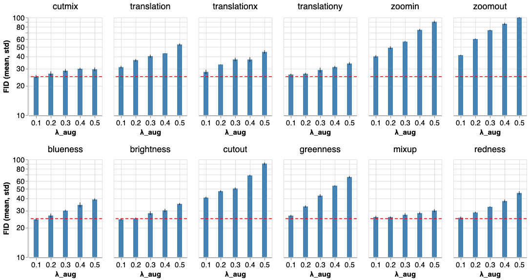
Figure 2: FID comparisons of SNDCGAN trained on augmented real images only. It shows only augmenting real images is not helpful with vanilla GAN training, which is consistent with the result in Section 4.1 of Zhang et al. [42]. Corresponding plots of BigGAN results are in the appendix.

We first compare the effect of image augmentations when only applied to the real images, the de-facto way of image augmentations in GANs [30, 4, 20]. Figure 2 illustrates the FID of the generated images with different strengths of each augmentation. We find augmenting only real images in GANs worsens the FID regardless of the augmentation strengths or strategies. For example, the baseline SNDCGAN trained without any image augmentation achieves 24.73 in FID [42], while translation, even with its smallest strength, gets 31.03. Moreover, FID increases monotonically as we increase the strength of the augmentation. This conclusion is surprising given the wide adoption of this conventional image augmentations in GANs. We note that the discriminator is likely to view the augmented data as part of the data distribution in such case. As shown by Figures 7, 8, 9 and 10 in the appendix, the generated images are prone to contain augmentation artifacts. Since FID is calculating the feature distance between generated samples and unaugmented real images, we believe the augmented artifacts in the synthesized samples are the underlying reason for the inferior FID.

3.2 Augmenting Both Real and Fake Images Improves GANs Consistently

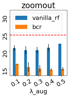
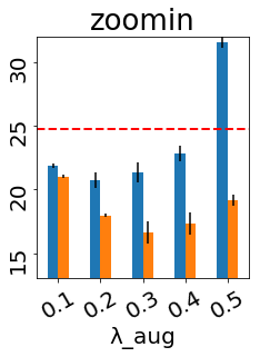
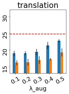
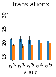
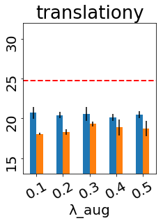
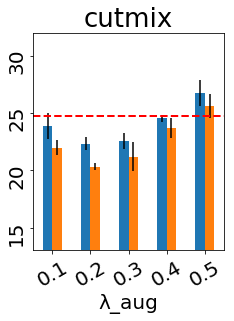
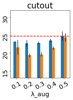
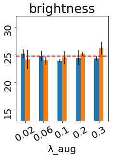
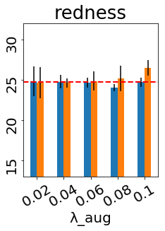
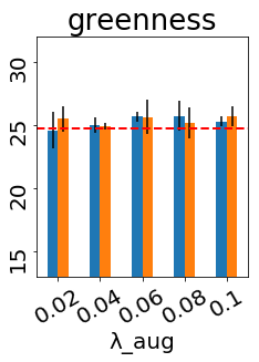
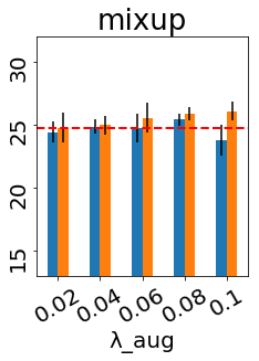
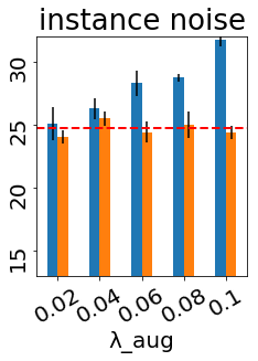
Figure 3: FID comparisons of SNDCGAN on CIFAR-10. The red dashed horizontal line shows the baseline FID=24.73 of SNDCGAN trained without data augmentation. ‘vanilla_rf’ (Section 3.2) represents training vanilla SNDCGAN and augmenting both real images as well as generated fake images concurrently before fed into the discriminator. And ‘bcr’ (Section 4) corresponds to training SNDCGAN with Balanced Consistency Regularization on augmented real and fake images. This figure can be utilized as general guidelines for training GAN with augmentations. The main implications are: (1) Simply augmenting real and fake images can make the vanilla GAN’s performance on par with recent proposed CR-GAN [42]. (2) With the help of BCR on augmented real and fake images, the generation fidelity can be improved by even larger margins. (3) Spatial augmentations outperform visual augmentations. (4) Augmentations that result in images out of the natural data manifold, e.g. InstanceNoise, cannot help with improving GAN performance.

Based on the above observation, it is natural to wonder whether augmenting generated images in the same way before feeding them into the discriminator can alleviate the problem. In this way, augmentation artifacts cannot be used to distinguish real and fake images by the discriminator.

To evaluate the augmentation of synthetic images, we train SNDCGAN and BigGAN by augmenting both real images as well as generated images concurrently before feeding them into the discriminator during training. Different from augmenting real images, we keep the gradients for augmented generated images to train the generator. The discriminator is now trained to differentiate between the augmented real image $t(\mathcal{I}_{\text{real}})$ and the augmented fake image $t(G(z))$. We present the generation FID of SNDCGAN and BigGAN in Figures 3 and 5 (denoted as ‘vanilla_rf’), where the horizontal lines show the baseline FIDs without any augmentations. As illustrated by Figure 3, this new augmentation strategy considerably improves the FID for different augmentations with varying strengths. By comparing the results in Figure 3 and Figure 2, we conclude that augmenting both real and fake images can substantially improves the generation performance of GAN. Moreover, for SNDCGAN, we find the best FID 18.94 achieved by translation of strength 0.1 is comparable to the FID 18.72 reported in Zhang et al. [42] with consistency regularization only on augmented real images. This observation holds for BigGAN as well, where we get FID 11.03 and the FID of CRGAN [42] is 11.48. These results suggest that image augmentations for both real and fake images considerably improve the training of vanilla GANs, which has not been studied by previous work, to our best knowledge.

We compare the effectiveness of augmentation operations in Figures 3 and 5. The operations in the top row such as translation, zoomin, and zoomout, are much more effective than the operations in the bottom rows, such as brightness, colorness, and mixup. We conclude that augmentations that result in spatial changes improve the GAN performance more than those that induce mostly visual changes.

3.3 Augmentations Increase the Support Overlap between Real and Fake Distributions

In this section, we investigate the reasons why augmenting both real and fake images improves GAN performance considerably. Roughly, GANs’ objective corresponds to making the generated image distribution close to real image distribution. However, as mentioned by previous work [35, 1], the difficulty of training GANs stems from these two being concentrated distributions whose support do not overlap: the real image distribution is often assumed to concentrate on or around a low-dimensional manifold, and similarly, generated image distribution is degenerate by construction. Therefore, Sønderby et al. [35] propose to add instance noise (i.e., Gaussian Noise) as augmentation for both real images and fakes image to increase the overlap of support between these two distributions. We argue that other semantic-preserving image augmentations have a similar effect to increase the overlap, and are much more effective for image generation.

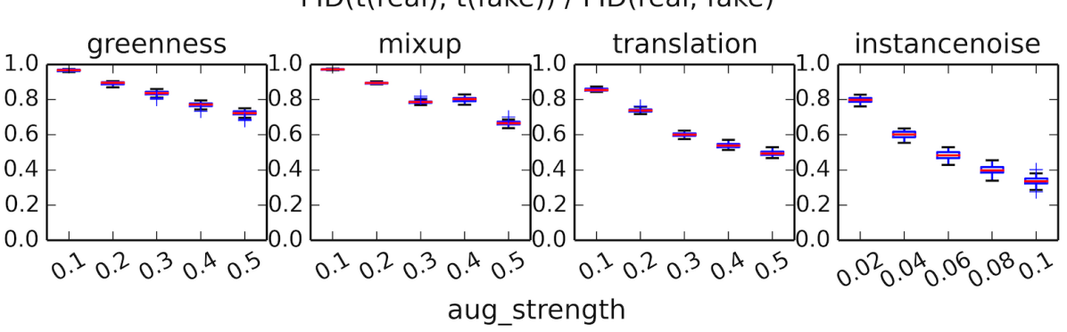
Figure 4: Distances between real and fake distributions with different augmentations. Note that we report $\text{FID}(\mathcal{I}_{\text{real}},\mathcal{I}_{\text{fake}})$ normally throughout the paper. While here to show the changes of real and fake image distributions with augmentations, we also calculate $\text{FID}(t(\mathcal{I}_{\text{real}}),t(\mathcal{I}_{\text{fake}}))$ and present its fraction over normal FID as y-axis. The Frechet Inception Distance between real and fake images gets smaller with augmentations, while stronger augmentations result in more distribution overlaps.

In Figure 4, we show that augmentations $t\sim\mathcal{T}$ can lower FID between augmented $t(\mathcal{I}_{\text{real}})$ and $t(\mathcal{I}_{\text{fake}})$, which indicates that the support of image distribution and the support of model distribution have more overlaps with augmentations. However, not all augmentations or strengths can improve the quality of generated images, which suggests naively pulling distribution together may not always improve the generation quality. We hypothesize certain types of augmentations and augmentations of high strengths can result in images that are far away from the natural image distribution; we leave the theoretical justification for future work.

4 Effect of Image Augmentations for Consistency Regularized GANs

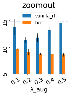
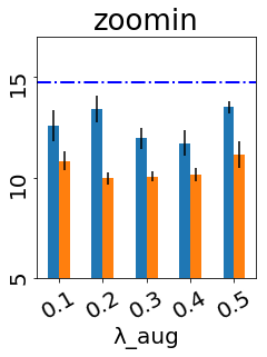
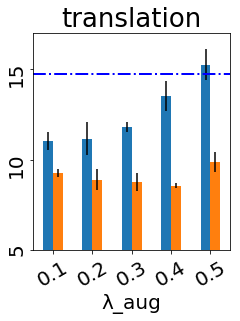
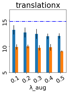
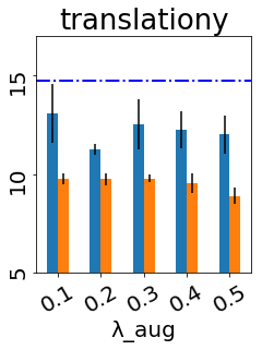
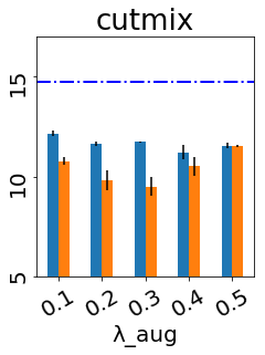
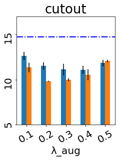
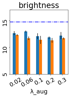
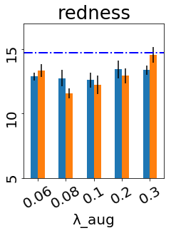
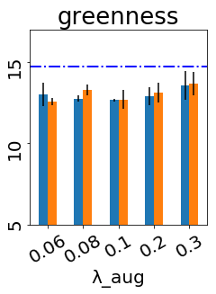
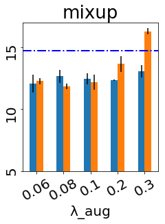
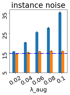
Figure 5: FID mean and std of BigGAN on CIFAR-10. The blue dashed horizontal line shows the baseline FID=14.73 of BigGAN trained without augmentation. ‘vanilla_rf’ (Section 3.2) represents training vanilla BigGAN with both real and fake images augmented. ‘bcr’ (Section 4) corresponds to training BigGAN with BCR on augmented real and fake images. This figure can be utilized as general guidelines for training GAN with augmentations, sharing similar implications as in Figure 3.

We now turn to more advanced regularized GANs that built on their usage of augmentations. Consistency Regularized GAN (CR-GAN) [42] has demonstrated that consistency regularization can significantly improve GAN training stability and generation performance. Zhao et al. [46] improves this method by introducing Balanced Consistency Regularization (BCR), which applying BCR to both real and fake images. Both methods requires images to be augmented for processing, and we briefly summarize BCR-GAN with Algorithm 1 in the appendix.

However, neither of the works studies the impact and importance of individual augmentation and only very basic geometric transformations are used as augmentation. We believe an in-depth analysis of augmentation techniques can strengthen the down-stream applications of consistency regularization in GANs. Here we mainly focus on analyzing the efficacy of different augmentations on BCR-GAN. We set the BCR strength $\lambda_{\text{BCR}}=10$ in Algorithm 1 according to the best practice. We present the generation FID of SNDCGAN and BigGAN with BCR on augmented real and fake images in Figures 3 and 5 (denoted as ‘bcr’), where the horizontal lines show the baseline FIDs without any augmentation. Experimental results suggest that consistency regularization on augmentations for real and fake images can further boost the generation performance.

More importantly, we can also significantly outperform the state of the art by carefully selecting the augmentation type and strength. For SNDCGAN, the best FID 14.72 is with zoomout of strength 0.4, while the corresponding FID reported in Zhao et al. [46] is 15.87 where basic translation of 4 pixels and flipping are applied. The best BigGAN FID 8.65 is with translation of strength 0.4, outperforming the corresponding FID 9.21 reported in Zhao et al. [46].

Similarly as in Section 3.2, augmentation techniques can be roughly categorized into two groups, in the descending order of effectiveness: spatial transforms, zoomout, zoomin, translation, translationx, translationy, cutout, cutmix; and visual transforms, brightness, redness, greenness, blueness, mixup. Spatial transforms, which retain the major content while introducing spatial variances, can substantially improve GAN performance together with BCR. On the other hand, instance noise [35], which may be able to help stabilize GAN training, cannot improve generation performance.

5 Effect of Images Augmentations for GANs with Contrastive Loss

Image augmentation is also an essential component of contrastive learning, which has recently led to substantially improved performance on self-supervised learning [7, 14]. Given the success of contrastive loss for representation learning and the success of consistency regularization in GANs, it naturally raises the question of whether adding such a regularization term helps in training GANs? In this section, we first demonstrate how we apply contrastive loss (CntrLoss) to regularizing GAN training. Then we analyze on how the performance of Cntr-GAN is affected by different augmentations, including variations of an augmentation set in existing work [7].

Contrastive Loss for GAN Training

The contrastive loss was originally introduced by Hadsell et al. [12] in such a way that corresponding positive pairs are pulled together while negative pairs are pushed apart. Here we propose Cntr-GAN, where contrastive loss is applied to regularizing the discriminator on two random augmented copies of both real and fake images. CntrLoss encourages the discriminator to push different image representations apart, while drawing augmentations of the same image closer. Due to space limit, we detail the CntrLoss in Appendix D and illustrate how our Cntr-GAN is trained with augmenting both real and fake images (Algorithm 2) in the appendix.

For augmentation techniques, we adopt and sample the augmentation as described in Chen et al. [7], referring it as simclr. Details of simclr augmentation can be found in the appendix (Section B). Due to the preference of large batch size for CntrLoss, we mainly experiment on BigGAN which has higher model capacity. As shown in Table 1, Cntr-GAN outperforms baseline BigGAN without any augmentation, but is inferior to BCR-GAN.

Table 1: BigGAN and regularizations.

Regularization	FID	InceptionScore
Vanilla	14.73	9.22 [4]
Cntr	12.27	9.23
BCR	9.21	9.29
Cntr+BCR	8.30	9.41

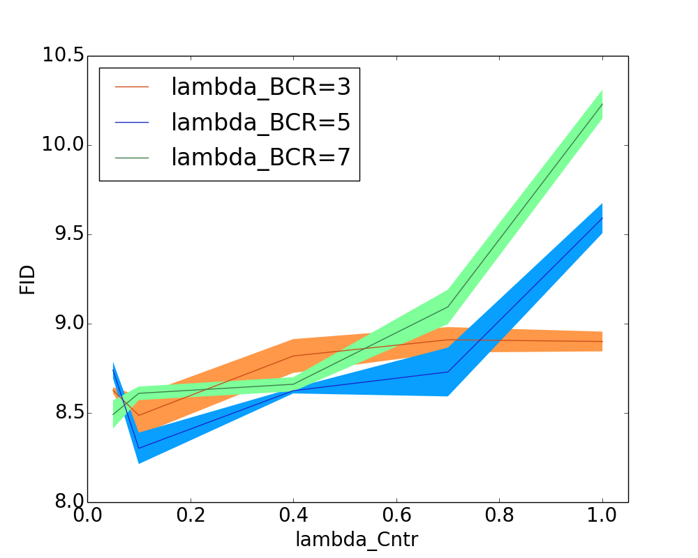
Figure 12: BigGAN on CIFAR-10 regularized with both Cntr and BCR. We achieve new state-of-the-art $\text{FID}=8.30$ with $\lambda_{\text{Cntr}}=0.1,\lambda_{\text{BCR}}=5$.

Since both BCR and CntrLoss utilize augmentations but are complementary in how they draw positive image pairs closer and push negative pairs apart, we further experiment on regularizing BigGAN with both CntrLoss and BCR. We are able to achieve new state-of-the-art $\text{FID}=8.30$ with $\lambda_{\text{Cntr}}=0.1,\lambda_{\text{BCR}}=5$. Table 1 compares the performance of vanilla BigGAN against BigGAN with different regularizations on augmentations, and Figure 12 in the appendix shows how the strengths affect the results. While BCR enforces the consistency loss directly on the discriminator logits, with Cntr together, it further helps to learn better representations which can be reflected in generation performance eventually.

Cntr-GAN Benefits From Stronger Augmentations

In Table 1, we adopt default augmenations in the literature for BCR [46] and CntrLoss [7]. Now we further study which image transform used by simclr affects Cntr-GAN the most, and also the effectiveness of the other augmentations we consider in this paper. We conducted extensive experiment on Cntr-GAN with different augmentations and report the most representative ones in Figure 6.

Overall, we find Cntr-GAN prefers stronger augmentation transforms compared to BCR-GAN. Spatial augmentations still work better than visual augmentations, which is consistent with our observation that changing the color jittering strength of simclr cannot help improve performance. In Figure 6, we present the results of changing the cropping/resizing strength in ‘simclr’, along with the other representative augmentation methods that are helpful to Cntr-GAN. For most augmentations, CntrGAN reaches the best performance with higher augmentation strength around 0.5. For CntrGAN, we achieve the best FID of 11.87 applying adjusted simclr augmentations with the cropping/resizing strength of 0.3.

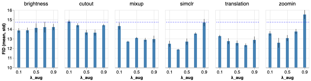
Figure 6: BigGAN regularized by CntrLoss with different image augmentations. The blue dashed horizontal line shows the baseline FID=14.73 of BigGAN trained without augmentation. Here we adjust the strength of cropping-resizing in the default simclr. Cntr-GAN consistently outperforms vanilla GAN with preferance on spatial augmentations.

6 Discussion

Here we provide additional analysis and discussion for several different aspects. Due to space limit, we summarize our findings below and include visualization of the results in the appendix.

Artifacts. Zhao et al. [46] show that imbalanced (only applied to real images) augmentations and regularizations can result in corresponding generation artifacts for GAN models. Therefore, we present qualitative images sampled randomly for different augmentations and settings of GAN training in the appendix (Section E). For vanilla GAN, augmenting both real and fake images can reduce generation artifacts substantially than only augmenting real images. With additional contrastive loss and consistency regularization, the generation quality can be improved further.

Annealing Augmentation Strength. We have extensively experimented with first setting $\lambda_{\text{aug}}$, which constrains the augmentation strength, then sampling augmentations randomly. But how would GANs’ performance change if we anneal $\lambda_{\text{aug}}$ during training? Our experiments show that annealing the strength of augmentations during training would reduce the effect of the augmentation, without changing the relative efficacy of different augmentations. Augmentations that improve GAN training would alleviate their improvements with annealing; and vice versa.

Composition of Transforms. Besides a single augmentation transform, the composition of multiple transforms are also used [8, 9, 16]. Though the dimension of random composition of transforms is out of this paper’s scope, we experiment with applying both translation and brightness, as spatial and visual transforms respectively, to BCR-GAN training. Preliminary results show that this chained augmentation can achieve the best FID=8.42, while with the single augmentation translation the best FID achieved is 8.58, which suggests this combination is dominant by the more effective translation. We leave it to future work to search for the best strategy of augmentation composition automatically.

7 Related Work

Data augmentation has shown to be critical to improve the robustness and generalization of deep learning models, and thus it is becoming an essential component of visual recognition systems  [22, 13, 7, 31, 47, 5, 45]. More recently, it also becomes one of the most impetus on semi-supervised learning and unsupervised learning [37, 2, 34, 38, 3, 7]. The augmentation operations also evolve from the basic random cropping and image mirroring to more complicated strategies including geometric distortions (e.g., changes in scale, translation and rotation), color jittering (e.g, perturbations in brightness, contrast and saturation) [8, 9, 44, 16] and combination of multiple image statistics [39, 43].

Nevertheless, these augmentations are still mainly studied in image classification tasks. As for image augmentations in GANs [11], the progress is very limited: from DCGAN [30] to BigGAN [4] and StyleGAN2 [20], the mainstream work is only using random cropping and horizontal flipping as the exclusive augmentation strategy. It remains unclear to the research community whether other augmentations can improve quality of generated samples. Recently, Zhang et al. [43] stabilized GAN training by mixing both the input and the label for real samples and generated ones. Sønderby et al. [35] added Gaussian noise to the input images and annealed its strength linearly during the training to achieve better convergence of GAN models. Arjovsky and Bottou [1] derived the same idea independently from a theoretical perspective. They have shown adding Gaussian noise to both real and fake images can alleviate training instability when the support of data distribution and model distribution do not overlap. Salimans et al. [33] further extended the idea by adding Gaussian noise to the output of each layer of the discriminator. Jahanian et al. [18] found data augmentation improves steerability of GAN models, but they failed to generate realistic samples on CIFAR-10 when jointly optimizing the model and linear walk parameters. Besides simply adding augmentation to the data, some recent work [6, 42, 46] further added the regularization on top of augmentations to improve the model performance. For example, Self-Supervised GANs [6, 28] make the discriminator to predict the angle of rotated images and CRGAN [42] enforce consistency for different image perturbations.

8 Conclusion

In this work, we have conducted a thorough analysis on the performance of different augmentations for improving generation quality of GANs. We have empirically shown adding the augmentation to both real images and generated samples is critical for producing realistic samples. Moreover, we observe that applying consistency regularization onto augmentations can further boost the performance and it is superior to applying contrastive loss. Finally, we achieve state-of-the-art image generation performance by combining constrastive loss and consistency loss. We hope our findings can lay a solid foundation and help ease the research in applying augmentations to wider applications of GANs.

Appendix A Notations

• $(H,W)$: height and width of an image $\mathcal{I}$

• $\lambda_{\text{aug}}$: augmentation strength

• $\mathcal{U}(\cdot,\cdot)$, $\mathcal{N}(\cdot,\cdot)$, and $\mathcal{B}(\cdot,\cdot)$: Uniform, Gaussian, and Beta distributions respectively.

• CR: consistency regularization [42]

• BCR: balanced consistency regularization [46]

• Cntr: contrastive loss [7]

• $G(z)$: generator output

• $D(x)$: discriminator output

• $D_{h}(x)$: hidden representation of discriminator output

• $f(D_{h}(x))$: projection head on top of hiddent representation

• $\mathcal{T}$: augmentation transforms

Appendix B Augmentations

ZoomIn: We sample $\alpha\sim\mathcal{U}(0,\lambda_{\text{aug}})$, randomly crop size $((1-\alpha)H,(1-\alpha)W)$ of the image, and resize the cropped image back to $(H,W)$ with bilinear interpolation.

ZoomOut: We sample $\alpha\sim\mathcal{U}(0,\lambda_{\text{aug}})$, evenly pad the image to size $((1+2\alpha)H,(1+2\alpha)W)$ with reflection, randomly crop size $((1+\alpha)H,(1+\alpha)W)$ of the image, and resize the cropped image back to $(H,W)$ with bilinear interpolation.

TranslationX: We sample $\alpha\sim\mathcal{U}(-\lambda_{\text{aug}},\lambda_{\text{aug}})$, and shift the image horizontally by $|\alpha|H$ in the direction of $\text{sign}(\alpha)$ with reflection padding.

TranslationY: We sample $\alpha\sim\mathcal{U}(-\lambda_{\text{aug}},\lambda_{\text{aug}})$, and shift the image vertically by $|\alpha|W$ in the direction of $\text{sign}(\alpha)$ with reflection padding.

Translation: We sample $\alpha_{h},\alpha_{w}\sim\mathcal{U}(-\lambda_{\text{aug}},\lambda_{\text{aug}})$, and shift the image vertically and horizontally by $|\alpha_{h}|H$ and $|\alpha_{w}|W$ in the direction of $\text{sign}(\alpha_{h})$ and $\text{sign}(\alpha_{w})$ with reflection padding.

Brightness: We sample $\alpha\sim\mathcal{U}(-\lambda_{\text{aug}},\lambda_{\text{aug}})$, add $\alpha$ to all channels and locations of the image, and clip pixel values to the range $[0,1]$.

Colorness: We sample $\alpha\sim\mathcal{U}(-\lambda_{\text{aug}},\lambda_{\text{aug}})$, add $\alpha$ to one of RGB channels of the image, and clip values to the range $[0,1]$.

InstanceNoise [35]: We add Gaussian noise $\mathcal{N}(0,\lambda_{\text{aug}})$ to the image. According to Sønderby et al. [35], we also anneal the noise variance from $\lambda_{\text{aug}}$ to 0 during training.

CutOut [10]: We sample $\alpha\sim\mathcal{U}(0,\lambda_{\text{aug}})$, and randomly mask out a $(\alpha H,\alpha W)$ region of the image with pixel value of 0.

CutMix [39]: We sample $\alpha\sim\mathcal{U}(0,\lambda_{\text{aug}})$, pick another random image $\mathcal{I}_{1}$ in the same batch, cut a patch of size $(\alpha H,\alpha W)$ from $\mathcal{I}_{1}$, and paste the patch to the corresponding region in $\mathcal{I}_{0}$.

MixUp [43]: We first sample $\alpha\sim\mathcal{B}(\lambda_{\text{aug}},\lambda_{\text{aug}})$, and set $\alpha=\max(\alpha,1-\alpha)$. Then we pick another random image $\mathcal{I}_{1}$ in the same batch, and use $t(\mathcal{I}_{0})=\alpha\mathcal{I}_{0}+(1-\alpha)\mathcal{I}_{1}$ as the augmented image.

SimCLR [7]: For the default simclr augmentation applied to our Cntr-GAN, we adopt the exact augmentations applied to CIFAR-10 in the opensource code  of [7]. The default simclr first crops the image with aspect ration in range [3/4, 4/3] and covered area in range [0.08, 1.0]. Then the crops are resized to the original image size, and applied with random horizontal flip. Finally, color jitters are applied changing the brightness, contrast, saturation, and hue of images. Please check code opensourced by Chen et al. [7] for more details.

Appendix C BCR-GAN: GAN with Balanced Consistency Regularization

Algorithm 1 Balanced Consistency Regularized GAN (BCR-GAN) [46]

  Input: parameters of generator $\theta_{G}$ and discriminator $\theta_{D}$, consistency regularization coefficient $\lambda_{\text{BCR}}$, augmentation transforms $\mathcal{T}$, assuming the discriminator updates only once per generator iteration.

  for number of training iterations do

     Sample batch $x\sim p_{\text{real}}(x)$, $z\sim p(z)$

     Real images $\mathcal{I}_{\text{real}}=x$, fake images $\mathcal{I}_{\text{fake}}=G(z)$

     $L_{D}\leftarrow D(\mathcal{I}_{\text{fake}})-D(\mathcal{I}_{\text{real}})$

     Sample augmentation transforms $t_{1}\sim\mathcal{T},t_{2}\sim\mathcal{T}$

     Augment both real and fake images $t_{1}(\mathcal{I}_{\text{real}}),t_{2}(\mathcal{I}_{\text{fake}})$

     $L_{\text{BCR}}\leftarrow\lVert D(\mathcal{I}_{\text{real}})-D(t_{1}(\mathcal{I}_{\text{real}}))\rVert^{2}+\lVert D(\mathcal{I}_{\text{fake}})-D(t_{2}(\mathcal{I}_{\text{fake}}))\rVert^{2}$

     $\theta_{D}\leftarrow\text{AdamOptimizer}(L_{D}+\lambda_{\text{BCR}}L_{\text{BCR}})$

     $L_{G}\leftarrow-D(G(z))$

     $\theta_{G}\leftarrow\text{AdamOptimizer}(L_{G})$

  end for

Appendix D Cntr-GAN: GAN with Contrastive Loss

We first elaborate on contrastive loss as defined in Chen et al. [7]. Given a minibatch representations of $N$ examples, and another minibatch representations of corresponding augmented examples, we concatenate them into a batch of $2N$ examples. After concatenation, a positive pair $(i,j)$ should have $|i-j|=N$, while we treat the other $2(N-1)$ samples within the batch as negative examples. Then the loss function for a positive pair of examples $(i,j)$ is defined as:

$$\ell_{i,j} =-\log\frac{\exp(\text{sim}(h_{i},h_{j})/\tau)}{\sum_{k=1}^{2N}\mathbbm{1}_{[k\neq i]}\exp(\text{sim}(h_{i},h_{k})/\tau)}$$

where $\text{sim}(u,v)=u^{T}v/\|u\|\|v\|$ denotes the cosine similarity between two vectors, $\mathbbm{1}_{[k\neq i]}\in\{0,1\}$ is an indicator evaluating to 1 iff $k\neq i$, and $\tau$ denotes a temperature hyper-parameter. The final contrastive loss (CntrLoss) is computed across all positive pairs, both $(i,j)$ and $(j,i)$ in the concatenated batch of size $2N$.

Then we propose Cntr-GAN, in which we apply contrastive loss to GANs with both real and fake images augmented during training. Algorithm 2 details how we augment images and regularize GAN training with CntrLoss.

Algorithm 2 Contrastive Loss regularized GAN (Cntr-GAN)

  Input: parameters of generator $\theta_{G}$ and discriminator $\theta_{D}$, $D_{h}($) returns the last hidden representation from the discriminator, $f($) is the projection head that maps representations to the space where contrastive loss is applied, contrastive loss coefficient $\lambda_{\text{Cntr}}$, augmentation transforms $\mathcal{T}$, assuming the discriminator updates only once per generator iteration.

  for number of training iterations do

     Sample batch $x\sim p_{\text{real}}(x)$, $z\sim p(z)$

     Real images $\mathcal{I}_{\text{real}}=x$, fake images $\mathcal{I}_{\text{fake}}=G(z)$

     $L_{D}\leftarrow D(\mathcal{I}_{\text{fake}})-D(\mathcal{I}_{\text{real}})$

     Sample augmentation transforms $t_{1}\sim\mathcal{T},t_{2}\sim\mathcal{T},t_{3}\sim\mathcal{T},t_{4}\sim\mathcal{T}$

     Augment both real and fake images $t_{1}(\mathcal{I}_{\text{real}}),t_{2}(\mathcal{I}_{\text{real}}),t_{3}(\mathcal{I}_{\text{fake}}),t_{4}(\mathcal{I}_{\text{fake}})$

     Obtain projected representations $h_{\text{real}1}=f(D_{h}(t_{1}(\mathcal{I}_{\text{real}}))),h_{\text{real}2}=f(D_{h}(t_{2}(\mathcal{I}_{\text{real}})))$

     $h_{\text{fake}1}=f(D_{h}(t_{3}(\mathcal{I}_{\text{fake}}))),h_{\text{fake}2}=f(D_{h}(t_{4}(\mathcal{I}_{\text{fake}})))$

     $L_{\text{Cntr}}\leftarrow\text{CntrLoss}(h_{\text{real}1},h_{\text{real}2})+\text{CntrLoss}(h_{\text{fake}1},h_{\text{fake}2})$

     $\theta_{D}\leftarrow\text{AdamOptimizer}(L_{D}+\lambda_{\text{Cntr}}L_{\text{Cntr}})$

     $L_{G}\leftarrow-D(G(z))$

     $\theta_{G}\leftarrow\text{AdamOptimizer}(L_{G})$

  end for

Appendix E Generation Artifacts

BigGAN w/ only $\mathcal{I}_{\text{real}}$ augmented, FID=29.23

BigGAN w/ $\mathcal{I}_{\text{real}}$ & $\mathcal{I}_{\text{fake}}$ augmented, FID=14.02

Cntr-BigGAN w/ $\mathcal{I}_{\text{real}}$ & $\mathcal{I}_{\text{fake}}$ augmented, FID=13.75

BCR-BigGAN w/ $\mathcal{I}_{\text{real}}$ & $\mathcal{I}_{\text{fake}}$ augmented, FID=13.19

Figure 7: Random qualitative examples showing brightness artifacts with $\lambda_{\text{aug}}=0.3$. For vanilla GAN, augmenting both real and fake images can reduce generation artifacts substantially than only augmenting real images. With additional contrastive loss and consistency regularization, the generation quality can be improved further.

BigGAN w/ only $\mathcal{I}_{\text{real}}$ augmented, FID=33.26

BigGAN w/ $\mathcal{I}_{\text{real}}$ & $\mathcal{I}_{\text{fake}}$ augmented, FID=16.52

Cntr-BigGAN w/ $\mathcal{I}_{\text{real}}$ & $\mathcal{I}_{\text{fake}}$ augmented, FID=15.57

BCR-BigGAN w/ $\mathcal{I}_{\text{real}}$ & $\mathcal{I}_{\text{fake}}$ augmented, FID=14.41

Figure 8: Random qualitative examples showing blueness artifacts with $\lambda_{\text{aug}}=0.3$. For vanilla GAN, augmenting both real and fake images can reduce generation artifacts substantially than only augmenting real images. With additional contrastive loss and consistency regularization, the generation quality can be improved further.

BigGAN w/ only $\mathcal{I}_{\text{real}}$ augmented, FID=50.98

BigGAN w/ $\mathcal{I}_{\text{real}}$ & $\mathcal{I}_{\text{fake}}$ augmented, FID=14.65

Cntr-BigGAN w/ $\mathcal{I}_{\text{real}}$ & $\mathcal{I}_{\text{fake}}$ augmented, FID=13.08

BCR-BigGAN w/ $\mathcal{I}_{\text{real}}$ & $\mathcal{I}_{\text{fake}}$ augmented, FID=11.66

Figure 9: Random qualitative examples showing zoomin artifacts with $\lambda_{\text{aug}}=0.3$. For vanilla GAN, augmenting both real and fake images can reduce generation artifacts substantially than only augmenting real images. With additional contrastive loss and consistency regularization, the generation quality can be improved further.

BigGAN w/ only $\mathcal{I}_{\text{real}}$ augmented, FID=47.76

BigGAN w/ $\mathcal{I}_{\text{real}}$ & $\mathcal{I}_{\text{fake}}$ augmented, FID=14.30

Cntr-BigGAN w/ $\mathcal{I}_{\text{real}}$ & $\mathcal{I}_{\text{fake}}$ augmented, FID=14.12

BCR-BigGAN w/ $\mathcal{I}_{\text{real}}$ & $\mathcal{I}_{\text{fake}}$ augmented, FID=12.63

Figure 10: Random qualitative examples showing cutout artifacts with $\lambda_{\text{aug}}=0.3$. For vanilla GAN, augmenting both real and fake images can reduce generation artifacts substantially than only augmenting real images. With additional contrastive loss and consistency regularization, the generation quality can be improved further.

Appendix F Additional Results

F.1 BigGAN with Only Real Images Augmented

As extra results for Section 3.1, the results of BigGAN with only real images augmented is consistent with Figure 2. It further shows only augmenting real images is not helpful with vanilla GAN.

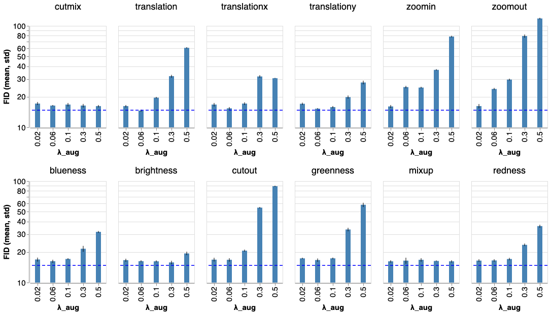
Figure 11: FID comparisons of BigGAN trained on augmented real images only.

F.2 Interaction between CntrLoss and BCR

In Section 5, we experiment with applying both CntrLoss and BCR to regularizing BigGAN. We achieve new state-of-the-art $\text{FID}=8.30$ with the strength of CntrLoss $\lambda_{\text{Cntr}}=0.1$ and the strength of BCR $\lambda_{\text{BCR}}=5$. While BCR enforces the consistency loss directly on the discriminator logits, with Cntr together, it further helps to learn better representations which can be reflected in generation performance eventually.

F.3 Annealing Augmentation Strength during Training

Our experiments show that annealing the strength of augmentations during training would reduce the effect of the augmentation, without changing the relative efficacy of different augmentations. Augmentations that improve GAN training would alleviate their improvements with annealing; and vice versa.

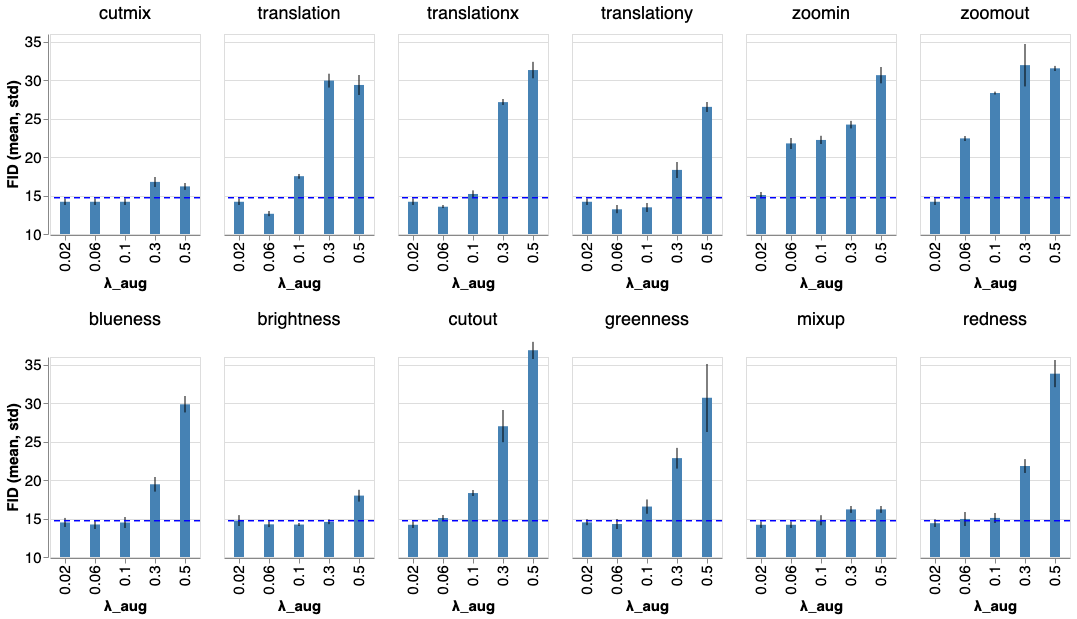
Figure 13: Annealing Augmentation Strength during Training.

F.4 Exploration on Chain of Augmentations

We experiment with applying both translation and brightness, as spatial and visual transforms respectively, to BCR-GAN training. Preliminary results show that this chained augmentation can achieve the best FID=8.42, while with the single augmentation translation the best FID achieved is 8.58. This suggests the combination of translation and brightness is dominant by the more effective translation. We leave it to future work to search for the best strategy of augmentation composition automatically.

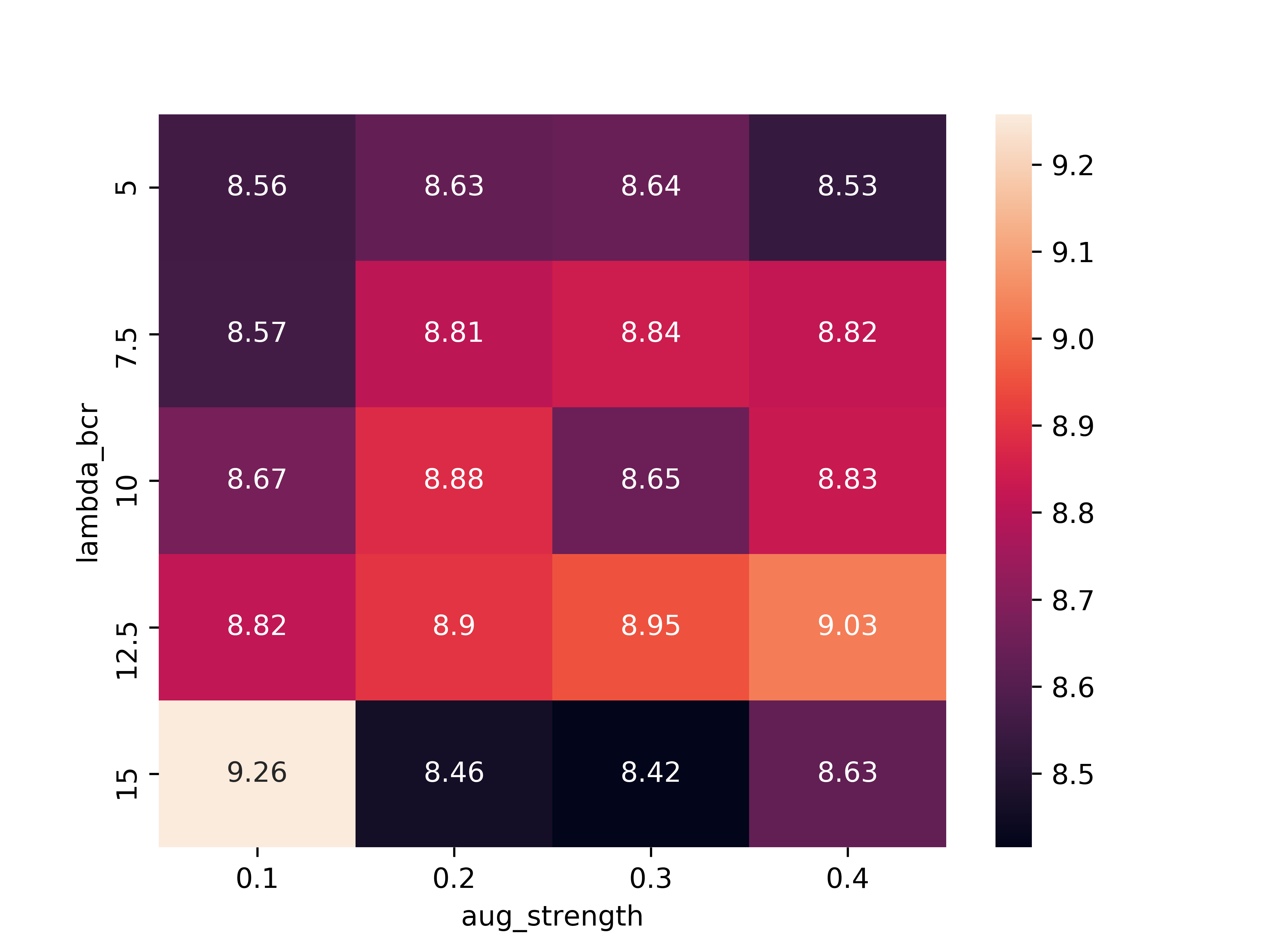
Figure 14: BCR with translation + brightness

Appendix G Model Details

Unconditional SNDCGAN

The SNDCGAN architecture is shown below. Please refer Kurach et al. [24] for more details.

Conditional BigGAN

The BigGAN architecture is shown below. Please refer Brock et al. [4] for more details.

References

- Arjovsky and Bottou [2017] Martín Arjovsky and Léon Bottou. Towards principled methods for training generative adversarial networks. In ICLR, 2017.
- Berthelot et al. [2019] David Berthelot, Nicholas Carlini, Ian Goodfellow, Nicolas Papernot, Avital Oliver, and Colin A Raffel. Mixmatch: A holistic approach to semi-supervised learning. In NeurIPS, 2019.
- Berthelot et al. [2020] David Berthelot, Nicholas Carlini, Ekin D. Cubuk, Alex Kurakin, Kihyuk Sohn, Han Zhang, and Colin Raffel. Remixmatch: Semi-supervised learning with distribution matching and augmentation anchoring. In ICLR, 2020.
- Brock et al. [2019] Andrew Brock, Jeff Donahue, and Karen Simonyan. Large scale gan training for high fidelity natural image synthesis. In ICLR, 2019.
- Chen et al. [2018] Liang-Chieh Chen, George Papandreou, Iasonas Kokkinos, Kevin Murphy, and Alan L. Yuille. Deeplab: Semantic image segmentation with deep convolutional nets, atrous convolution, and fully connected crfs. IEEE Trans. Pattern Anal. Mach. Intell., 40(4):834–848, 2018.
- Chen et al. [2019] Ting Chen, Xiaohua Zhai, Marvin Ritter, Mario Lucic, and Neil Houlsby. Self-supervised gans via auxiliary rotation loss. In CVPR, 2019.
- Chen et al. [2020] Ting Chen, Simon Kornblith, Mohammad Norouzi, and Geoffrey Hinton. A simple framework for contrastive learning of visual representations. arXiv preprint arXiv:2002.05709, 2020.
- Cubuk et al. [2019a] Ekin D. Cubuk, Barret Zoph, Dandelion Mane, Vijay Vasudevan, and Quoc V. Le. Autoaugment: Learning augmentation strategies from data. In CVPR, 2019a.
- Cubuk et al. [2019b] Ekin D Cubuk, Barret Zoph, Jonathon Shlens, and Quoc V Le. Randaugment: Practical automated data augmentation with a reduced search space. arXiv preprint arXiv:1909.13719, 2019b.
- DeVries and Taylor [2017] Terrance DeVries and Graham W Taylor. Improved regularization of convolutional neural networks with cutout. arXiv preprint arXiv:1708.04552, 2017.
- Goodfellow et al. [2014] Ian Goodfellow, Jean Pouget-Abadie, Mehdi Mirza, Bing Xu, David Warde-Farley, Sherjil Ozair, Aaron Courville, and Yoshua Bengio. Generative adversarial nets. In Advances in Neural Information Processing Systems, pages 2672–2680, 2014.
- Hadsell et al. [2006] Raia Hadsell, Sumit Chopra, and Yann LeCun. Dimensionality reduction by learning an invariant mapping. In 2006 IEEE Computer Society Conference on Computer Vision and Pattern Recognition (CVPR’06), volume 2, pages 1735–1742. IEEE, 2006.
- He et al. [2016] Kaiming He, Xiangyu Zhang, Shaoqing Ren, and Jian Sun. Deep residual learning for image recognition. In CVPR, 2016.
- He et al. [2019] Kaiming He, Haoqi Fan, Yuxin Wu, Saining Xie, and Ross Girshick. Momentum contrast for unsupervised visual representation learning. arXiv preprint arXiv:1911.05722, 2019.
- He et al. [2020] Kaiming He, Georgia Gkioxari, Piotr Dollár, and Ross B. Girshick. Mask R-CNN. IEEE Trans. Pattern Anal. Mach. Intell., 42(2):386–397, 2020.
- Hendrycks et al. [2020] Dan Hendrycks, Norman Mu, Ekin Dogus Cubuk, Barret Zoph, Justin Gilmer, and Balaji Lakshminarayanan. Augmix: A simple data processing method to improve robustness and uncertainty. In ICLR, 2020.
- Heusel et al. [2017] Martin Heusel, Hubert Ramsauer, Thomas Unterthiner, Bernhard Nessler, and Sepp Hochreiter. Gans trained by a two time-scale update rule converge to a local nash equilibrium. In NeurIPS, 2017.
- Jahanian et al. [2020] Ali Jahanian, Lucy Chai, and Phillip Isola. On the "steerability" of generative adversarial networks. In ICLR, 2020.
- Karras et al. [2019a] Tero Karras, Samuli Laine, and Timo Aila. A style-based generator architecture for generative adversarial networks. In Proceedings of the IEEE Conference on Computer Vision and Pattern Recognition, pages 4401–4410, 2019a.
- Karras et al. [2019b] Tero Karras, Samuli Laine, Miika Aittala, Janne Hellsten, Jaakko Lehtinen, and Timo Aila. Analyzing and improving the image quality of stylegan. arXiv preprint arXiv:1912.04958, 2019b.
- Krizhevsky et al. [2009] Alex Krizhevsky, Geoffrey Hinton, et al. Learning multiple layers of features from tiny images. Citeseer, 2009.
- Krizhevsky et al. [2012] Alex Krizhevsky, Ilya Sutskever, and Geoffrey E. Hinton. Imagenet classification with deep convolutional neural networks. In NeurIPS, 2012.
- Kurach et al. [2019a] Karol Kurach, Mario Lucic, Xiaohua Zhai, Marcin Michalski, and Sylvain Gelly. A large-scale study on regularization and normalization in gans. In ICML, 2019a.
- Kurach et al. [2019b] Karol Kurach, Mario Lucic, Xiaohua Zhai, Marcin Michalski, and Sylvain Gelly. A large-scale study on regularization and normalization in gans. In ICML, 2019b.
- Laine and Aila [2016] Samuli Laine and Timo Aila. Temporal ensembling for semi-supervised learning. arXiv preprint arXiv:1610.02242, 2016.
- Lim and Ye [2017] Jae Hyun Lim and Jong Chul Ye. Geometric GAN. arXiv:1705.02894, 2017.
- Lucic et al. [2018] Mario Lucic, Karol Kurach, Marcin Michalski, Sylvain Gelly, and Olivier Bousquet. Are gans created equal? A large-scale study. In NeurIPS, 2018.
- Lucic et al. [2019] Mario Lucic, Michael Tschannen, Marvin Ritter, Xiaohua Zhai, Olivier Bachem, and Sylvain Gelly. High-fidelity image generation with fewer labels. In ICML, 2019.
- Miyato et al. [2018] Takeru Miyato, Toshiki Kataoka, Masanori Koyama, and Yuichi Yoshida. Spectral normalization for generative adversarial networks. In ICLR, 2018.
- Radford et al. [2016] Alec Radford, Luke Metz, and Soumith Chintala. Unsupervised representation learning with deep convolutional generative adversarial networks. In ICLR, 2016.
- Ren et al. [2015] Shaoqing Ren, Kaiming He, Ross B. Girshick, and Jian Sun. Faster R-CNN: towards real-time object detection with region proposal networks. In NeurIPS, 2015.
- Sajjadi et al. [2016] Mehdi Sajjadi, Mehran Javanmardi, and Tolga Tasdizen. Regularization with stochastic transformations and perturbations for deep semi-supervised learning. In NeurIPS, 2016.
- Salimans et al. [2016] Tim Salimans, Ian Goodfellow, Wojciech Zaremba, Vicki Cheung, Alec Radford, and Xi Chen. Improved techniques for training gans. In NeurIPS, 2016.
- Sohn et al. [2020] Kihyuk Sohn, David Berthelot, Chun-Liang Li, Zizhao Zhang, Nicholas Carlini, Ekin D Cubuk, Alex Kurakin, Han Zhang, and Colin Raffel. Fixmatch: Simplifying semi-supervised learning with consistency and confidence. arXiv preprint arXiv:2001.07685, 2020.
- Sønderby et al. [2017] Casper Kaae Sønderby, Jose Caballero, Lucas Theis, Wenzhe Shi, and Ferenc Huszár. Amortised map inference for image super-resolution. In ICLR, 2017.
- Tran et al. [2017] Dustin Tran, Rajesh Ranganath, and David M. Blei. Deep and hierarchical implicit models. arXiv:1702.08896, 2017.
- Xie et al. [2019a] Qizhe Xie, Zihang Dai, Eduard Hovy, Minh-Thang Luong, and Quoc V Le. Unsupervised data augmentation for consistency training. arXiv preprint arXiv:1904.12848, 2019a.
- Xie et al. [2019b] Qizhe Xie, Eduard Hovy, Minh-Thang Luong, and Quoc V Le. Self-training with noisy student improves imagenet classification. arXiv preprint arXiv:1911.04252, 2019b.
- Yun et al. [2019] Sangdoo Yun, Dongyoon Han, Seong Joon Oh, Sanghyuk Chun, Junsuk Choe, and Youngjoon Yoo. Cutmix: Regularization strategy to train strong classifiers with localizable features. In Proceedings of the IEEE International Conference on Computer Vision, pages 6023–6032, 2019.
- Zhang et al. [2017] Han Zhang, Tao Xu, Hongsheng Li, Shaoting Zhang, Xiaogang Wang, Xiaolei Huang, and Dimitris N Metaxas. Stackgan: Text to photo-realistic image synthesis with stacked generative adversarial networks. In Proceedings of the IEEE international conference on computer vision, pages 5907–5915, 2017.
- Zhang et al. [2019] Han Zhang, Ian Goodfellow, Dimitris Metaxas, and Augustus Odena. Self-attention generative adversarial networks. In ICML, 2019.
- Zhang et al. [2020a] Han Zhang, Zizhao Zhang, Augustus Odena, and Honglak Lee. Consistency regularization for generative adversarial networks. In ICLR, 2020a.
- Zhang et al. [2018] Hongyi Zhang, Moustapha Cisse, Yann N Dauphin, and David Lopez-Paz. mixup: Beyond empirical risk minimization. In ICLR, 2018.
- Zhang et al. [2020b] Xinyu Zhang, Qiang Wang, Jian Zhang, and Zhao Zhong. Adversarial autoaugment. In ICLR, 2020b.
- Zhao et al. [2018] Zhengli Zhao, Dheeru Dua, and Sameer Singh. Generating natural adversarial examples. In International Conference on Learning Representations (ICLR), 2018.
- Zhao et al. [2020] Zhengli Zhao, Sameer Singh, Honglak Lee, Zizhao Zhang, Augustus Odena, and Han Zhang. Improved consistency regularization for gans. arXiv preprint arXiv:2002.04724, 2020.
- Zoph et al. [2019] Barret Zoph, Ekin D. Cubuk, Golnaz Ghiasi, Tsung-Yi Lin, Jonathon Shlens, and Quoc V. Le. Learning data augmentation strategies for object detection. CoRR, abs/1906.11172, 2019.