Local SGD With a Communication Overhead Depending Only on the Number of Workers

Abstract

We consider speeding up stochastic gradient descent (SGD) by parallelizing it across multiple workers. We assume the same data set is shared among $n$ workers, who can take SGD steps and coordinate with a central server. Unfortunately, this could require a lot of communication between the workers and the server, which can dramatically reduce the gains from parallelism. The Local SGD method, proposed and analyzed in the earlier literature, suggests machines should make many local steps between such communications. While the initial analysis of Local SGD showed it needs $\Omega(\sqrt{T})$ communications for $T$ local gradient steps in order for the error to scale proportionately to $1/(nT)$, this has been successively improved in a string of papers, with the state-of-the-art requiring $\Omega\left(n\left(\mbox{ polynomial in log }(T)\right)\right)$ communications. In this paper, we give a new analysis of Local SGD. A consequence of our analysis is that Local SGD can achieve an error that scales as $1/(nT)$ with only a fixed number of communications independent of $T$: specifically, only $\Omega(n)$ communications are required.

1 Introduction

Stochastic Gradient Descent (SGD) is a widely used algorithm to minimize a convex or non-convex function $F$ in which model parameters are updated iteratively as follows:

$${\mathbf{x}}^{t+1}={\mathbf{x}}^{t}-\eta_{t}\hat{\mathbf{g}}^{t},$$

where $\hat{\mathbf{g}}^{t}$ is a stochastic gradient of $F$ at ${\mathbf{x}}^{t}$ and $\eta_{t}$ is the learning rate. This algorithm can be naively parallelized by adding more workers independently to compute a gradient and then average them at each step to reduce the variance in estimation of the true gradient $\nabla F({\mathbf{x}}^{t})$ [DGBSX12]. This method requires each worker to share their computed gradients with each other at every iteration.

However, it is widely acknowledged that communication is a major bottleneck of this method for large scale optimization applications [MMR⁺17, KMY⁺16, LHM⁺18]. Often, mini-batch parallel SGD is suggested to address this issue by increasing the computation to communication ratio. Nonetheless, too large mini-batch size might degrades the performance [LSPJ18]. Along the same lines of increasing compute to communication, local SGD has been proposed to reduce communications [MMR⁺17, DP19]. In this method, workers compute (stochastic) gradients and update their parameters locally, and communicate only once in a while to obtain the average of their parameters. Local SGD improves the communication efficiency not only by reducing the number of communication rounds, but also alleviates the synchronization delay caused by waiting for slow workers and evens out the variations in workers’ computing time [WJ18b].

On the other hand, since individual gradients of each worker are calculated at different points, this method introduces residual error as opposed to fully synchronous SGD. Therefore, there is a trade-off between having fewer communication rounds and introducing additional errors to the gradient estimates.

The idea of making local updates is not new and has been used in practice for a while [KMY⁺16]. However, until recently, there have been few successful efforts to analyze Local SGD theoretically and therefore it is not fully understood yet. The paper [ZDSMR16] shows that for quadratic functions, when the variance of the noise is higher far from the optimum, frequent averaging leads to faster convergence. One of the main questions we want to ask is: how many communication rounds are needed for Local SGD to have the same convergence rate of a synchronized parallel SGD while achieving performance that linearly improves in the number of workers?

[Sti19] was among the earlier works that tried to answer this question for general strongly convex and smooth functions and showed that the communication rounds can be reduced up to a factor of $H=\mathcal{O}(\sqrt{T/n})$, without affecting the asymptotic convergence rate (up to constant factors), where $T$ is the total number of iterations and $n$ is number of parallel workers.

Focusing on smooth and possibly non-convex functions which satisfy a Polyak-Lojasiewicz condition, [HKMC19] demonstrates that only $R=\Omega((Tn)^{1/3})$ communication rounds are sufficient to achieve asymptotic performance that scales proportionately to $1/n$.

More recently, [KMR20] and [SK19] improve upon the previous works by showing linear-speed up for Local SGD with only $\Omega\left(n\mbox{ poly log }(T)\right)$ communication rounds when data is identically distributed among workers and $F$ is strongly convex. Their works also consider the cases when $F$ is not necessarily strongly-convex as well as the case of data being heterogeneously distributed among workers in [KMR20].

Table 1: Comparison of Similar Works

[b] noise model $H=T$ ^a convergent communication rounds, $R$ convergence rate, $F(\hat{\mathbf{x}}^{t})-F^{*}$ Reference uniform no $\Omega(\sqrt{Tn})$ $\mathcal{O}(\frac{\xi^{0}}{R^{3}}+\frac{\sigma^{2}}{\mu nT}+\frac{\kappa G^{2}}{\mu R^{2}})$ ^b [Sti19] uniform with strong-growth ^c no $\Omega((Tn)^{1/3})$ $\mathcal{O}(\frac{\xi^{0}}{R^{3}}+\frac{\kappa\sigma^{2}}{\mu nT}+\frac{\kappa^{2}\sigma^{2}}{\mu nTR})$ [HKMC19] uniform with strong-growth no $\Omega(n*\text{poly-log}(T))$ $\tilde{\mathcal{O}}(\frac{\kappa nH\xi^{0}}{\exp(R/(\kappa n))}+\frac{\sigma^{2}}{\mu nT})$ ^d [SK19] uniform yes $\Omega(n*\text{poly-log}(T))$ $\tilde{\mathcal{O}}(\frac{\kappa\xi^{0}}{T^{2}}+\frac{\kappa\sigma^{2}}{n\mu T}+\frac{\kappa^{2}\sigma^{2}}{\mu TR})$ [KMR20] uniform with strong-growth yes $\Omega(n)$ $\mathcal{O}(\frac{\kappa^{4}\ln(TR^{-2})\xi^{0}}{T^{2}}+\frac{\kappa\sigma^{2}}{\mu nT}+\frac{\kappa^{2}\sigma^{2}}{\mu TR})$ This Paper

• $H$ is the length of inter-communication intervals.

• $G$ is the uniform upper bound assumed for the $l_{2}$ norm of gradients in the corresponding work.

• This noise model is defined in Assumption 2.

• $\tilde{\mathcal{O}}(.)$ ignores the poly-logarithmic and constant factors.

In this work, we focus on smooth and strongly-convex functions with a very general noise model. The main contribution of this paper is to propose a communication strategy which requires only $R=\Omega(n)$ communication rounds to achieve performance that scales as $1/n$ in the number of workers. To the best of the authors’ knowledge, this is the only work to show this result (without additional poly-logarithmic terms and constants). Our analysis can also recover some of the best known rates for special cases, e.g., when $H$ is constant, where $H$ is defined as the length of intercommunication intervals. A summary of our results compared to the available literature can be found in Table 1.

The rest of this paper is organized as follows. In the following subsection we outline the related literature and ongoing works. In Section 2 we define the main problem and state our assumptions. We present our theoretical findings in Section 3 and the sketch of proofs in Section 4, followed by numerical experiments in Section 5 and conclusion remarks in Section 6.

1.1 Related Works

There has been a lot of effort in the recent research to take into account the communication delays and training time in designing faster algorithms [MHM10, ZCL15, BSS16, KMA⁺19]. See [TSC⁺20] for a comprehensive survey of communication efficient distributed training algorithms considering both system-level and algorithm-level optimizations.

Many works study the communication complexity of distributed methods for convex optimization [AS15] [WPS⁺20] and statistical estimation [ZDJW13]. [WPS⁺20] presents a rigorous comparison of Local SGD with $H$ local steps and mini-batch SGD with $H$ times larger mini-batch size and the same number of communication rounds (we will refer to such a method as large mini-batch SGD) and show regimes in which each algorithm performs better: they show that Local SGD is strictly better than large mini-batch SGD when the functions are quadratic. Moreover, they prove a lower bound on the worst case of Local SGD that is higher than the worst-case error of large mini-batch SGD in a certain regime. [ZDJW13] studies the minimum amount of communication required to achieve centralized minimax-optimal rates by establishing lower bounds on minimax risks for distributed statistical estimation under a communication budget.

A parallel line of work studies the convergence of Local SGD with non-convex functions [ZC18]. [YYZ19] was among the first works to present provable guarantees of Local SGD with linear speed up. [WJ18b] and [KLB⁺20] present unified frameworks for analyzing decentralized SGD with local updates, elastic averaging or changing topology. The follow-up work [WJ18a] presents ADACOMM, an adaptive communication strategy that starts with infrequent averaging and then increases the communication frequency in order to achieve a low error floor. They analyze the error-runtime trade-off of Local SGD with nonconvex functions and propose communication times to achieve faster runtime.

In One-Shot Averaging (OSA), workers perform local updates with no communication during the optimization until the end when they average their parameters. This method can be seen as an extreme case of Local SGD with $H=T$, on the opposite end of synchronous SGD [MMS⁺09, ZWLS10, ZDW13, RN16, GBS20]. [DP19] provides non-asymptotic analysis of mini-batch SGD and one-shot averaging as well as regimes in which mini-batch SGD could outperform one-shot averaging.

Another line of work reduces the communication by compressing the gradients and hence limiting the number of bits transmitted in every message between workers [LHM⁺18, AGL⁺17, WWLZ18, SCJ18, SK19].

Asynchronous methods have been studied widely due to their advantages over synchronous methods which suffer from synchronization delays due to the slower workers [SOP20]. [WSY⁺19] studies the error-runtime trade-off in decentralized optimization and proposes MATCHA, an algorithm which parallelizes inter-node communication by decomposing the topology into matchings. [HBM19] provides an accelerated stochastic algorithm for decentralized optimization of finite-sum objective functions that by carefully balancing the ratio between communications and computations match the rates of the best known sequential algorithms while having the network scaling of optimal batch algorithms. However, these methods are relatively more involved and they often require full knowledge of the network, solving a semi-definite program and/or calculating communication probabilities (schedules).

1.2 Notation

For a positive integer $s$, we define $[s]:=\{1,\ldots,s\}$. We use bold letters to represent vectors. We denote vectors of all $0$s and $1$s by $\mathbf{0}$ and $\mathbf{1}$, respectively. We use $\|\cdot\|$ for the Euclidean norm.

2 Problem Formulation

Suppose there are $n$ workers ${\mathcal{V}}=\{1,\ldots,n\}$, trying to minimize $F:\mathbb{R}^{d}\rightarrow\mathbb{R}$ in parallel. We assume all workers have access to $F$ through noisy gradients. In Local SGD, workers perform local gradient steps and occasionally calculate the average of all workers’ iterates.

Having access to the same objective function $F$ is of special interest if the data is stored in one place accessible to all machines or is distributed identically among workers with no memory constraints. We hope that results presented here can be extended to applications with heterogeneous data distributions [KMR20].

We will make the following additional assumptions.

Assumption 1.

Function $F:\mathbb{R}^{d}\rightarrow\mathbb{R}$ is differentiable, $\mu$-strongly convex and $L$-smooth for $L\geq\mu>0$. In particular,

$$\frac{\mu}{2}\|{\mathbf{x}}-{\mathbf{y}}\|^{2}\leq F({\mathbf{y}})-F({\mathbf{x}})-\langle\nabla F({\mathbf{x}}),{\mathbf{y}}-{\mathbf{x}}\rangle\leq\frac{L}{2}\|{\mathbf{x}}-{\mathbf{y}}\|^{2},\qquad\forall x,y\in\mathbb{R}^{d}.$$

We define $\kappa=L/\mu$ to be the condition number of $F$.

We make the following assumption on the noise of the stochastic gradients.

Assumption 2.

Each worker $i$ has access to a gradient oracle which returns an unbiased estimate of the true gradient in the form $\hat{\mathbf{g}}_{i}({\mathbf{x}})=\nabla F({\mathbf{x}})+\boldsymbol{\epsilon}_{i}$, such that $\boldsymbol{\epsilon}_{i}$ is a zero-mean conditionally independent random noise with its expected squared norm error bounded as

$$\mathbb{E}[\boldsymbol{\epsilon}_{i}]=\mathbf{0},\qquad\mathbb{E}[\|\boldsymbol{\epsilon}_{i}\|^{2}|{\mathbf{x}}]\leq c\|\nabla F({\mathbf{x}})\|^{2}+\sigma^{2},$$

where $\sigma^{2},c\geq 0$ are constants.

To save space, we define $\hat{\mathbf{g}}_{i}^{t}:=\hat{\mathbf{g}}({\mathbf{x}}_{i}^{t})$ as the stochastic gradient of node $i$ at iteration $t$, and ${\mathbf{g}}_{i}^{t}=\nabla F({\mathbf{x}}_{i}^{t})$ as the true gradient at the same point.

The noise model of Assumption 2 is very general and it includes the common case with uniformly bounded squared norm error when $c=0$. As it is noted by [ZDSMR16], the advantage of periodic averaging compared to one-shot averaging only appears when $c/\sigma^{2}$ is large. Therefore, to study Local SGD, it is important to consider a noise model as in Assumption 2 to capture the effects of frequent averaging. Among the related works mentioned in Table 1, only [SK19] and [HKMC19] analyze this noise model while the rest study the special case with $c=0$. SGD under this noise model with $c>0$ and $\sigma^{2}=0$ was first studied in [SR13] under the name strong-growth condition. Therefore we refer to the noise model considered in this work as uniform with strong-growth.

In Local SGD, each worker $i$ holds a local parameter ${\mathbf{x}}_{i}^{t}$ at iteration $t$ and a set ${\mathcal{I}}\subset[T]$ of communication times, and performs the following update:

$${\mathbf{x}}_{i}^{t+1}=\begin{cases}x_{i}^{t}-\eta_{t}\hat{\mathbf{g}}_{i}^{t},\qquad&\text{if }t+1\notin{\mathcal{I}},\\ \frac{1}{n}\sum_{j=1}^{n}({\mathbf{x}}_{j}^{t}-\eta_{t}\hat{\mathbf{g}}_{j}^{t}),\qquad&\text{if }t+1\in{\mathcal{I}}.\end{cases}$$ (1)

When ${\mathcal{I}}=[T]$, we recover the fully synchronized parallel SGD, while ${\mathcal{I}}=\{T\}$ recovers one-shot averaging. The pseudo code for Local SGD is provided as Algorithm 1.

Algorithm 1 Local SGD

1:  Input ${\mathbf{x}}_{i}^{0}={\mathbf{x}}^{0}$ for $i\in[n]$, total number of iterations $T$, the step-size sequence $\{\eta_{t}\}_{t=0}^{T-1}$ and ${\mathcal{I}}\subseteq[T]$

2:  for $t=0,\ldots,T-1$ do

3:     for $j=1,\ldots,n$ do

4:        evaluate a stochastic gradient $\hat{\mathbf{g}}_{j}^{t}$

5:        if $t+1\in\mathcal{I}$ then

6:           ${\mathbf{x}}_{j}^{t+1}=\frac{1}{n}\sum_{i=1}^{n}({\mathbf{x}}_{i}^{t}-\eta_{t}\hat{\mathbf{g}}_{i}^{t})$

7:        else

8:           ${\mathbf{x}}_{j}^{t+1}={\mathbf{x}}_{j}^{t}-\eta_{t}\hat{\mathbf{g}}_{j}^{t}$

9:        end if

10:     end for

11:  end for

The main goal of this paper is to study the effect of communication times on the convergence of the Local SGD and provide better theoretical guarantees. In what follows, we claim that by carefully choosing the step size, linear speed-up of parallel SGD can be attained with only a small number of communication instances.

3 Convergence Results

In this section we present our convergence results for Local SGD. In the following theorem, we show an upper bound for the sub-optimality error, in the sense of function value, for any choice of communication times ${\mathcal{I}}$.

Before proceeding with our results, let us introduce some notation. Let $0=\tau_{0}<\tau_{1}<\ldots<\tau_{R}=T$ be the communication times. Define $H_{i}:=\tau_{i+1}-\tau_{i}$, as the length of $i+1$-th inter-communication interval, for $i=0,\ldots,k-1$. Moreover, define $\bar{\mathbf{x}}^{t}:=(\sum_{i=1}^{n}{\mathbf{x}}_{i}^{t})/n$ as the the average of the iterates of all workers. Notice that ${\mathbf{x}}_{i}^{t}=\bar{\mathbf{x}}^{t}$ for $t\in{\mathcal{I}}$.

The main results of this paper will be obtained by specializing the following bound.

Theorem 1.

Suppose Assumptions 1 and 2 hold. Choose $\beta\geq 2\kappa^{2}$ and communication times ${\mathcal{I}}=\{\tau_{i}|i=1,\ldots,R\}$ such that it holds

$$9\kappa^{2}c\ln(1+\frac{H_{i}-1}{\tau_{i}+\beta})+2\kappa(1+\frac{c}{n})-(\tau_{i}+1+\beta)\leq 0,\qquad i=0,\ldots,R-1.$$ (2)

Set $\eta_{k}=2/(\mu(k+\beta))$. Then, using Algorithm 1, we have

$$\mathbb{E}[F(\bar{\mathbf{x}}^{T})]-F^{*}\leq\frac{\beta^{2}(F(\bar{\mathbf{x}}^{0})-F^{*})}{T^{2}}+\frac{2L\sigma^{2}}{n\mu^{2}T}+\frac{9L^{2}\sigma^{2}}{\mu^{3}T^{2}}\sum_{t=0}^{T-1}\frac{t-\tau(t)}{t+\beta},$$ (3)

where $F^{*}:=\min_{{\mathbf{x}}}F({\mathbf{x}})$ and $\tau(t):=\max\{t^{\prime}\in\mathcal{I}|t^{\prime}\leq t\}$ is the most recent communication time.

The last term in Equation (3) is due the to disagreement between workers (consensus error), introduced by local computations without any communication. As the inter-communication intervals become larger, $t-\tau(t)$ becomes larger as well and increases the overall optimization error. This term explains the trade-off between communication efficiency and the optimization error.

Note that condition (2) is mild. For instance, it suffices to set $\beta\geq\max\{9\kappa^{2}c\ln(1+T/(2\kappa^{2}))+2\kappa(1+c/n),2\kappa^{2}\}$. Moreover, the bound in (3) is for the last iterate $T$, and does not require keeping track of a weighted average of all the iterates.

Theorem 1 not only bounds the optimization error, but introduces a methodological approach to select the communication times to achieve smaller errors. For the scenarios when the user can afford to have a certain number of a communications, they can select $\tau_{i}$ to minimize the last term in (3).

We next discuss the implications of Theorem 1 under various conditions.

One-Shot Averaging.

Plugging $H=T$ in Theorem 1, we obtain a convergence rate of $\mathcal{O}(\kappa^{2}\sigma^{2}/(\mu T))$ without any linear speed-up. Among previous works, only [KMR20] shows a similar result.

3.1 Fixed-Length Intervals

A simple way to select the communication times ${\mathcal{I}}$, is to split the whole training time $T$ to $R$ intervals of length at most $H$. Then we can use the following bound in Equation (3),

$$\sum_{t=0}^{T-1}\frac{t-\tau(t)}{t+\beta}\leq(H-1)\sum_{t=0}^{T-1}\frac{1}{t+\beta}\leq(H-1)\ln(1+\frac{T}{\beta-1}).$$

We state this result formally in the following corollary.

Corollary 1.

Suppose assumptions of Theorem 1 hold and in addition, workers communicate at least once every $H$ iterations. Then,

$$\mathbb{E}[F(\bar{\mathbf{x}}^{T})]-F^{*}\leq\frac{\beta^{2}(F(\bar{\mathbf{x}}^{0})-F^{*})}{T^{2}}+\frac{2L\sigma^{2}}{n\mu^{2}T}+\frac{9L^{2}\sigma^{2}(H-1)}{\mu^{3}T^{2}}\ln(1+\frac{T}{\beta-1}).$$ (4)

Linear Speed-Up.

Setting $H=\mathcal{O}(T/(n\ln(T)))$ we achieve linear-speed up in the number of workers, which is equivalent to a communication complexity of $R=\Omega(n\ln(T))$. To the best of the authors’ knowledge, this is the tightest communication complexity that is shown to achieve linear speed-up. [KMR20] and [SK19] have shown a similar communication complexity, however with slightly higher degrees of dependence on $\ln(T)$, e.g., $R=\Omega(n\ln(T)^{2})$ in [KMR20].

Recovering Synchronized SGD.

When $H=1$, the the last term in (4) disappears and we recover the convergence rate of parallel SGD, albeit, with a worse dependence on $\kappa$.

3.2 Varying Intervals

In the previous subsection, we observed that with our current analysis, having fixed-length inter-communication intervals, linear speed-up can be achieved with only $\Omega(n\ln(T))$ rounds of communications. A natural question that might arise is whether we can improve the result above even further.

Let us allow consecutive inter-communication intervals, i.e., $H_{i}:=\tau_{i+1}-\tau_{i}$, grow linearly, where $0=\tau_{0}<\tau_{1}<\ldots<\tau_{R}=T$ are the communication times. The following Theorem presents a performance guarantee for this choice of communication times.

Theorem 2.

Suppose Assumptions 1 and 2 hold. Choose the maximum number of communications $1\leq R\leq\sqrt{2T}$ and set $a:=\lceil 2T/R^{2}\rceil\geq 1$, $H_{i}=a(i+1)$ and $\tau_{i+1}=\min(\tau_{i}+H_{i},T)$ for $i=0,\ldots,R-1$. Choose $\beta\geq\max\{2\kappa^{2},9\kappa^{2}c\max\{\ln(3),\ln(1+T/(R^{2}\kappa^{2}))\}+2\kappa(1+c/n)\}$ and set $\eta_{t}=2/\mu(t+\beta)$. Then using Algorithm 1 we have,

$$\mathbb{E}[F(\bar{\mathbf{x}}^{T})]-F^{*}\leq\frac{\beta^{2}(F(\bar{\mathbf{x}}^{0})-F^{*})}{T^{2}}+\frac{2L\sigma^{2}}{n\mu^{2}T}+\frac{72L^{2}\sigma^{2}}{\mu^{3}TR}.$$ (5)

The choice of communication times in Theorem 2 aligns with the intuition that workers need to communicate more frequently at the beginning of the optimization. As the the step-sizes become smaller and workers’ local parameters get closer to the global minimum, they diverge more slowly from each other and, hence, less communication is required to re-align them.

Linear Speed-Up.

Choosing communication rounds $R=\Omega(n)$, we achieve an error that scales as $1/(nT)$ in the number of workers when $T=\Omega(n^{2})$. This is the main result of this paper: it shows that we can get a linear speedup in the number of workers by simply increasing the number of iterations while keeping the total number of communications bounded.

4 Sketch of Proof

Here we give an outline of the proofs for the results presented in this paper. The proof of the following lemmas are left to the Appendix.

Perturbed Iterates.

A common approach in analyzing parallel algorithms such as Local SGD is to study the evolution of the sequence $\{\bar{\mathbf{x}}^{t}\}_{t\geq 0}$. We have,

$$\bar{\mathbf{x}}^{t+1}=\bar{\mathbf{x}}^{t}-\frac{\eta_{t}}{n}\sum_{i=1}^{n}\hat{\mathbf{g}}_{i}^{t}=\bar{\mathbf{x}}^{t}-\eta_{t}\tilde{\mathbf{g}}^{t},$$ (6)

where $\tilde{\mathbf{g}}^{t}:=(\sum_{i=1}^{n}\hat{\mathbf{g}}_{i}^{t})/n$ is the average of the stochastic gradient estimates of all workers.

Let us define $\xi^{t}:=\mathbb{E}[F(\bar{\mathbf{x}}^{t})]-F^{*}$ to be the optimality error. The following lemma, which is similar to a part of the proof found in [HKMC19], bounds the optimality error at each iteration recursively.

Lemma 1.

Let Assumptions 1 and 2 hold. Then,

$$\xi^{t+1}\leq\xi^{t}(1-\mu\eta_{t})+\frac{L^{2}\eta_{t}}{2n}\mathbb{E}\left[\sum_{i=1}^{n}\|\bar{\mathbf{x}}^{t}-{\mathbf{x}}_{i}^{t}\|^{2}\right]+\frac{\eta_{t}^{2}L}{2}\mathbb{E}[\|\tilde{\mathbf{g}}^{t}\|_{2}^{2}]-\frac{\eta_{t}}{2n}\mathbb{E}\left[\sum_{i=1}^{n}\|\nabla F({\mathbf{x}}_{i}^{t})\|^{2}\right].$$

Equipped with Lemma 1, we can bound the consensus error ($\mathbb{E}[\sum_{i=1}^{n}\|\bar{\mathbf{x}}^{t}-{\mathbf{x}}_{i}^{t}\|^{2}]$) as well as the term $\mathbb{E}[\|\tilde{\mathbf{g}}^{t}\|^{2}]$ in the following lemmas.

Consensus Error.

In the following lemmas, we utilize the structure of the problem to bound the consensus error recursively.

Lemma 2.

Let Assumptions 1 and 2 hold. Then,

$$\mathbb{E}\left[\sum_{i=1}^{n}\|{\mathbf{x}}_{i}^{t+1}-\bar{\mathbf{x}}^{t+1}\|^{2}\right]\leq\mathbb{E}\left[\sum_{i=1}^{n}\|{\mathbf{x}}_{i}^{t}-\bar{\mathbf{x}}^{t}\|^{2}\right](1-2\eta_{t}\mu+\eta_{t}^{2}L^{2})\\ +(n-1)\eta_{t}^{2}\sigma^{2}+(1-\frac{1}{n})\eta_{t}^{2}c\mathbb{E}[\sum_{i=1}^{n}\|g_{i}^{t}\|^{2}].$$ (7)

This lemma, bounds how much the consensus error grows at each iteration. Of course, when workers communicate, this error resets to zero and thus, we can calculate an upper bound for the consensus error, knowing the last iteration communication occurred and the step-size sequence. The following lemma takes care of that. Before stating the following lemma, let us define $G^{t}:=\frac{1}{n}\sum_{i=1}^{n}\|{\mathbf{g}}_{i}^{t}\|^{2}$.

Lemma 3.

Let assumptions of Theorem 1 hold. Then,

$$\mathbb{E}\left[\sum_{i=1}^{n}\|{\mathbf{x}}_{i}^{t}-\bar{\mathbf{x}}^{t}\|^{2}\right]\leq 9(n-1)\sum_{k=\tau(t)}^{t-1}\frac{c\mathbb{E}[G^{k}]+\sigma^{2}}{\mu^{2}(t+\beta)^{2}}.$$ (8)

Variance.

Our next lemma bounds $E[\|\tilde{\mathbf{g}}^{t}\|^{2}]$.

Lemma 4.

Under Assumption 2 we have,

$$\mathbb{E}[\|\tilde{\mathbf{g}}^{t}\|^{2}]\leq(1+\frac{c}{n})\mathbb{E}[G^{t}]+\frac{\sigma^{2}}{n}.$$

The proofs of Theorems 1 and 2 follow from these lemmas. Due to space constraints, these proofs are given in the supplementary information.

5 Numerical Experiments

To verify our findings and compare different communication strategies in Local SGD, we performed the following numerical experiments.

5.1 Quadratic Function With Strong-Growth Condition

As discussed in [ZDSMR16, DP19], under uniformly bounded variance, one-shot averaging performs asymptotically as well as mini-batch SGD. Therefore, to fully capture the importance of the choice of communication times ${\mathcal{I}}$, we design a hard problem, where noise variance is uniform with strong-growth condition, defined in Assumption 2. Let us define $F({\mathbf{x}})=\mathbb{E}_{\zeta}f({\mathbf{x}},\zeta)$ where,

$$f({\mathbf{x}},\zeta):=\sum_{i=1}^{d}\frac{1}{2}x_{i}^{2}(1+z_{1,i})+{\mathbf{x}}^{\top}{\mathbf{z}}_{2},$$ (9)

$\zeta=({\mathbf{z}}_{1},{\mathbf{z}}_{2})$, where ${\mathbf{z}}_{1},{\mathbf{z}}_{2}\in\mathbb{R}^{d},z_{1,i}\sim\mathcal{N}(0,c_{1})$ and $z_{2,i}\sim\mathcal{N}(0,c_{2})$, $\forall i\in[d]$ are random variables with normal distributions. We assume at each iteration $t$, each worker $i$ samples a $\zeta_{i}^{t}$ and uses $\nabla f({\mathbf{x}},\zeta_{i}^{t})$ as a stochastic estimate of $\nabla F({\mathbf{x}})$. It is easy to verify that $F({\mathbf{x}})=(1/2){\mathbf{x}}^{2}$ is $1$-strongly convex, $F^{*}=0$ and $\mathbb{E}_{\zeta}[\|\nabla f({\mathbf{x}},\zeta)-\nabla F({\mathbf{x}})\|^{2}]=c\|\nabla F({\mathbf{x}})\|^{2}+\sigma^{2}$, where $c=c_{1}$ and $\sigma^{2}=dc_{2}$.

We use Local SGD to minimize $F({\mathbf{x}})$ using different communication strategies. We select $c_{1}=9,c_{2}=0.25,d=3$, $n=20$ machines and $T=1000$ iterations and the step-size sequence $\eta_{t}=2/\mu(t+\beta)$ with $\beta=1$. We start each simulation from the initial point of ${\mathbf{x}}^{0}=\mathbf{1}_{d}$ and repeat each simulation $500$ times. The average of the results are reported in Figures 1(a) and 1(b). Moreover, average performance of Local SGD with different number of workers $n$ and the communication strategy proposed in this paper with $R=n$ is shown in Figure 1(c) along with the respective convergence rate of $\sigma^{2}/(\mu nt)$.

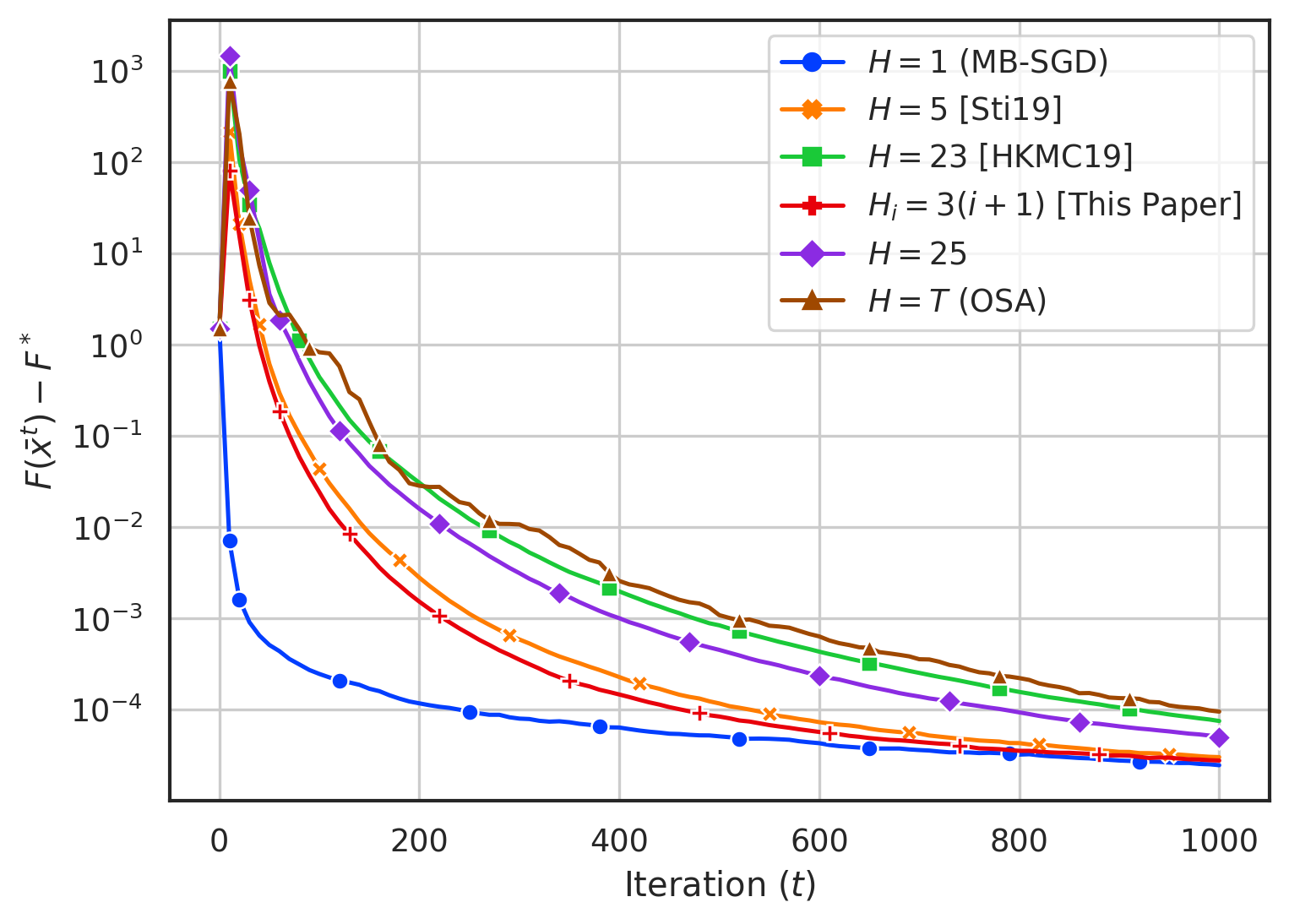
(a) Error over iterations.

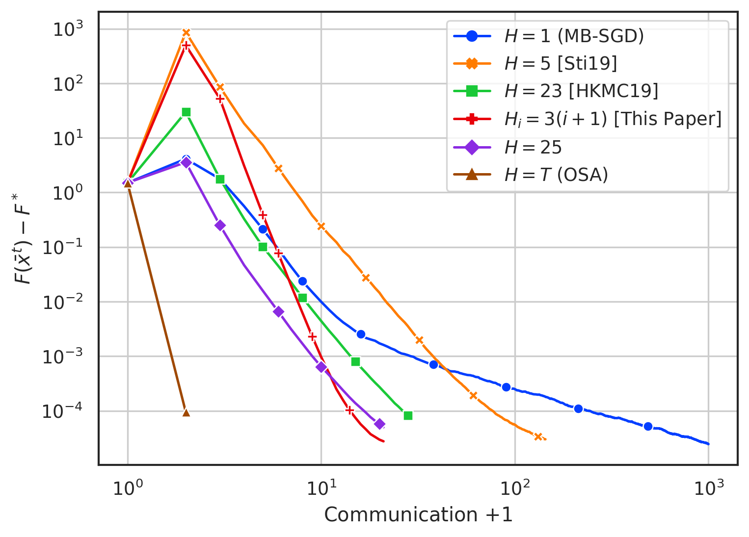
(b) Error over communications.

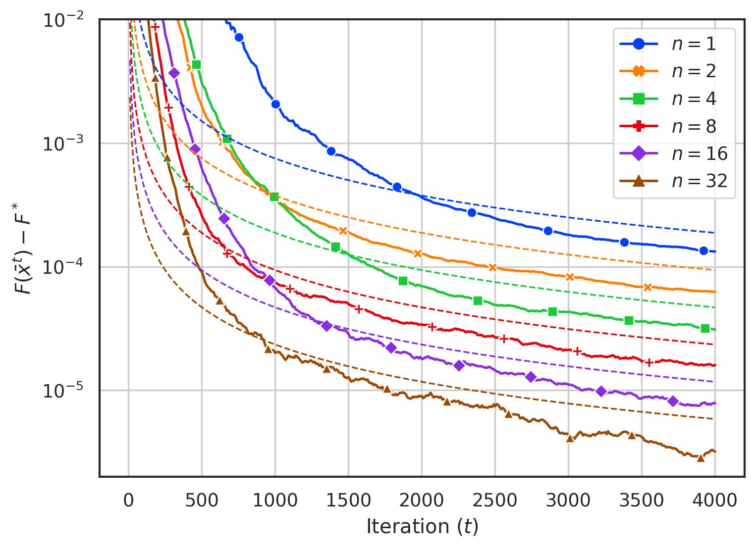
(c) Speed-up in the network size.

Figure 1: Local SGD with different communication strategies with $F({\mathbf{x}})=\mathbb{E}_{\zeta}f({\mathbf{x}},\zeta)$ defined in (9), $c=9,\sigma=0.5,d=3,\beta=1$. Figures (a) and (b) show the error of different communication methods over iteration and communication round, respectively, with a fixed network size of $n=20$. Figure (c) shows the convergence of Local SGD with the communication method proposed in this paper ($n$ communication rounds) for different network sizes. The dashed lines are showing $\sigma^{2}/(\mu nt)$.

Figure 1(a) shows that the method with increasing communication intervals ($H_{i}=3(i+1)$) proposed in this paper performs better than all the other communication strategies in the transient time as well as in the final error, requiring much less communication rounds. In particular, the method with the same number of communications but fixed intervals ($H=25$), has both higher transient error and final error. This affirms the advantages of having more frequent communication at the beginning of the optimization. Indeed, observe that in Figures 1(a), the only method which outperforms the method we propose is the one that communicates at every step.

Figure 1(b) reveals the effectiveness of each communication round in different methods. We observe that there’s an initial spike in the initial communications in methods $H=5$ and $H_{i}=3(i+1)$. This is mainly because these two methods have more frequent communications at the beginning of the training, where the step-sizes are larger. Other methods experience this increase as well, however since they communicate later, it’s not observed in this figure. Indeed, observe that the only method which makes better use of communication periods than our method in Figure 1(b) is one-shot averaging, which is not competitive in terms of its final error.

Figure 1(c) verifies that linear-speed up in the number of workers can be achieved with only $R=n$ communication rounds. Moreover, it shows that Local SGD achieves the optimal convergence rate of $\sigma^{2}/(n\mu T)$ asymptotically.

5.2 Regularized Logistic Regression

We also performed additional numerical experiments with regularized logistic regression using two real data sets. Due to space constraints, the results are presented in supplementary information.

6 Conclusion

We have presented a new analysis of Local SGD and studied the effect of choice of communication times on the final optimality error. We proposed a communication strategy which achieves linear speed-up in the number of workers with only $\Omega(n)$ communication rounds, independent of the total number of iterations $T$. Numerical experiments further confirmed our theoretical findings, and showed that our method achieves smaller error than previous methods using fewer communications.

Broader Impact

The results presented in this paper could help speed up training in many machine learning applications. The potential broader impacts are therefore somewhat generic for machine learning: this research could amplify all the benefits ML can bring by making it cheaper in terms of computational cost, while simultaneously amplifying all the ways ML could be misused.

Appendix A Missing Proofs

Let us define the following notations used in the proofs presented here.

$$\bar{\mathbf{g}}^{t}:=(\sum_{i=1}^{n}{\mathbf{g}}_{i}^{t})/n,\qquad G^{t}:=\frac{1}{n}\sum_{i=1}^{n}\|{\mathbf{g}}_{i}^{t}\|^{2},\qquad \boldsymbol{\epsilon}_{i}^{t}:=\hat{\mathbf{g}}_{i}^{t}-{\mathbf{g}}_{i}^{t}.$$

Moreover, define ${\mathcal{F}}^{t}:=\{{\mathbf{x}}_{i}^{k},\hat{\mathbf{g}}_{i}^{k}|1\leq i\leq n,0\leq k\leq t-1\}\cup\{{\mathbf{x}}_{i}^{t}|1\leq i\leq n\}$.

Lemma (1).

Let Assumptions 1 and 2 hold. Then,

$$\xi^{t+1}\leq\xi^{t}(1-\mu\eta_{t})+\frac{L^{2}\eta_{t}}{2n}\mathbb{E}\left[\sum_{i=1}^{n}\|\bar{\mathbf{x}}^{t}-{\mathbf{x}}_{i}^{t}\|^{2}\right]+\frac{\eta_{t}^{2}L}{2}\mathbb{E}[\|\tilde{\mathbf{g}}^{t}\|_{2}^{2}]-\frac{\eta_{t}}{2n}\mathbb{E}\left[\sum_{i=1}^{n}\|\nabla F({\mathbf{x}}_{i}^{t})\|^{2}\right].$$

Proof of Lemma 1.

By Assumption 1 and (6) we have,

$$\mathbb{E}[F(\bar{\mathbf{x}}^{t+1})-F(\bar{\mathbf{x}}^{t})]\leq-\eta_{t}\mathbb{E}[\langle\nabla F(\bar{\mathbf{x}}^{t}),\tilde{\mathbf{g}}^{t}\rangle]+\frac{\eta_{t}^{2}L}{2}\mathbb{E}[\|\tilde{\mathbf{g}}^{t}\|_{2}^{2}].$$ (10)

We bound the first term on the R.H.S of (10) by conditioning on ${\mathcal{F}}^{t}$ as follows:

$$\mathbb{E}[\langle\nabla F(\bar{\mathbf{x}}^{t}),\tilde{\mathbf{g}}^{t}\rangle|\mathcal{F}^{t}] =\frac{1}{n}\sum_{i=1}^{n}\langle\nabla F(\bar{\mathbf{x}}^{t}),\mathbb{E}[\hat{\mathbf{g}}_{i}^{t}|{\mathbf{x}}_{i}^{t}]\rangle$$

$$=\frac{1}{2}\|\nabla F(\bar{\mathbf{x}}^{t})\|^{2}+\frac{1}{2n}\sum_{i=1}^{n}\|\nabla F({\mathbf{x}}_{i}^{t})\|^{2}-\frac{1}{2n}\sum_{i=1}^{n}\|\nabla F(\bar{\mathbf{x}}^{t})-\nabla F({\mathbf{x}}_{i}^{t})\|^{2}$$

$$\geq\mu(F(\bar{\mathbf{x}}^{t})-F^{*})+\frac{1}{2n}\sum_{i=1}^{n}\|\nabla F({\mathbf{x}}_{i}^{t})\|^{2}-\frac{L^{2}}{2n}\sum_{i=1}^{n}\|\bar{\mathbf{x}}^{t}-{\mathbf{x}}_{i}^{t}\|^{2},$$ (11)

where we used $\langle a,b\rangle=\frac{1}{2}\|a\|^{2}+\frac{1}{2}\|b\|^{2}-\frac{1}{2}\|a-b\|^{2}$ in the second equation and $(1/2)\|\nabla F({\mathbf{x}})\|^{2}\geq\mu(F({\mathbf{x}})-F^{*})$ as well as smoothness of $F$ in the last inequality. Taking full expectation of (A) and combining it with (10) concludes the lemma. ∎

We state an important identity in the following lemma.

Lemma 5.

Let ${\mathbf{u}}_{1},\ldots{\mathbf{u}}_{n}\in\mathbb{R}^{d}$ be $n$ arbitrary vectors. Define $\bar{\mathbf{u}}=(\sum_{i=1}^{n}{\mathbf{u}}_{i})/n$. Then,

$$\sum_{i=1}^{n}\|{\mathbf{u}}_{i}-\bar{\mathbf{u}}\|^{2}=\sum_{i=1}^{n}\|{\mathbf{u}}_{i}\|^{2}-n\|\bar{\mathbf{u}}\|^{2}.$$

Proof.

We have

$$\sum_{i=1}^{n}\|{\mathbf{u}}_{i}-\bar{\mathbf{u}}\|^{2} =\sum_{i=1}^{n}\|{\mathbf{u}}_{i}\|^{2}+n\|\bar{\mathbf{u}}\|^{2}-2\sum_{i=1}^{n}\langle{\mathbf{u}}_{i},\bar{\mathbf{u}}\rangle$$

$$=\sum_{i=1}^{n}\|{\mathbf{u}}_{i}\|^{2}+n\|\bar{\mathbf{u}}\|^{2}-2n\langle\bar{\mathbf{u}},\bar{\mathbf{u}}\rangle$$

$$=\sum_{i=1}^{n}\|{\mathbf{u}}_{i}\|^{2}-n\|\bar{\mathbf{u}}\|^{2}.$$

∎

Lemma (2).

Let Assumptions 1 and 2 hold. Then,

$$\mathbb{E}\left[\sum_{i=1}^{n}\|{\mathbf{x}}_{i}^{t+1}-\bar{\mathbf{x}}^{t+1}\|^{2}\right]\leq\mathbb{E}\left[\sum_{i=1}^{n}\|{\mathbf{x}}_{i}^{t}-\bar{\mathbf{x}}^{t}\|^{2}\right](1-2\eta_{t}\mu+\eta_{t}^{2}L^{2})\\ +(n-1)\eta_{t}^{2}\sigma^{2}+(1-\frac{1}{n})\eta_{t}^{2}c\mathbb{E}[\sum_{i=1}^{n}\|g_{i}^{t}\|^{2}].$$

Proof of Lemma 2.

We have,

$$\mathbb{E}[\sum_{i=1}^{n}\|{\mathbf{x}}_{i}^{t+1}-\bar{\mathbf{x}}^{t+1}\|^{2}]=\sum_{i=1}^{n}\|\mathbb{E}[{\mathbf{x}}_{i}^{t+1}-\bar{\mathbf{x}}^{t+1}]\|^{2}+\sum_{i=1}^{n}\mathbb{E}\left[\|{\mathbf{x}}_{i}^{t+1}-\bar{\mathbf{x}}^{t+1}-\mathbb{E}[{\mathbf{x}}_{i}^{t+1}-\bar{\mathbf{x}}^{t+1}]\|^{2}\right].$$ (12)

Let us consider the first term on the right hand side of (12). Taking conditional expectation of both sides of (6) implies,

$$\sum_{i=1}^{n}\|\mathbb{E}[{\mathbf{x}}_{i}^{t+1}-\bar{\mathbf{x}}^{t+1}|\ {\mathcal{F}}^{t}]\|^{2} =\sum_{i=1}^{n}\|{\mathbf{x}}_{i}^{t}-\bar{\mathbf{x}}^{t}-\eta_{t}({\mathbf{g}}_{i}^{t}-\bar{\mathbf{g}}^{t})\|^{2}$$

$$=\sum_{i=1}^{n}\left(\|{\mathbf{x}}_{i}^{t}-\bar{\mathbf{x}}^{t}\|^{2}+\eta_{t}^{2}\|{\mathbf{g}}_{i}^{t}-\bar{\mathbf{g}}^{t}\|^{2}-2\eta_{t}\langle{\mathbf{g}}_{i}^{t},{\mathbf{x}}_{i}^{t}-\bar{\mathbf{x}}^{t}\rangle\right)$$ (13)

By $L$-smoothness of $F$,

$$\sum_{i=1}^{n}\|{\mathbf{g}}_{i}^{t}-\bar{\mathbf{g}}^{t}\|^{2}=\frac{1}{n}\sum_{\{i,j\}}\|{\mathbf{g}}_{i}^{t}-{\mathbf{g}}_{j}^{t}\|^{2}\leq\frac{L^{2}}{n}\sum_{\{i,j\}}\|{\mathbf{x}}_{i}^{t}-{\mathbf{x}}_{j}^{t}\|^{2}=L^{2}\sum_{i=1}^{n}\|{\mathbf{x}}_{i}^{t}-\bar{\mathbf{x}}^{t}\|^{2}.$$ (14)

Moreover, by $\mu$-strong convexity of $F$,

$$\sum_{i=1}^{n}\langle{\mathbf{g}}_{i}^{t},{\mathbf{x}}_{i}^{t}-\bar{\mathbf{x}}^{t}\rangle=\sum_{i=1}^{n}\langle{\mathbf{g}}_{i}^{t},\frac{1}{n}\sum_{j=1}^{n}({\mathbf{x}}_{i}^{t}-{\mathbf{x}}_{j}^{t})\rangle\\ =\frac{1}{n}\sum_{\{i,j\}}\langle{\mathbf{g}}_{i}^{t}-{\mathbf{g}}_{j}^{t},{\mathbf{x}}_{i}^{t}-{\mathbf{x}}_{j}^{t}\rangle\geq\frac{\mu}{n}\sum_{\{i,j\}}\|{\mathbf{x}}_{i}-{\mathbf{x}}_{j}\|^{2}=\mu\sum_{i=1}^{n}\|{\mathbf{x}}_{i}^{t}-\bar{\mathbf{x}}^{t}\|^{2},$$ (15)

where we used $\langle\nabla F({\mathbf{x}})-\nabla F({\mathbf{y}}),{\mathbf{x}}-{\mathbf{y}}\rangle\geq\mu\|{\mathbf{x}}-{\mathbf{y}}\|^{2}$ in the inequality. Combining (A)-(15) we obtain,

$$\sum_{i=1}^{n}\|\mathbb{E}[{\mathbf{x}}_{i}^{t+1}-\bar{\mathbf{x}}^{t+1}|{\mathcal{F}}^{t}]\|^{2} \leq\sum_{i=1}^{n}\|{\mathbf{x}}_{i}^{t}-\bar{\mathbf{x}}^{t}\|^{2}\left(1-2\eta_{t}\mu+\eta_{t}^{2}L^{2}\right),$$

Now, consider the second term on the right hand side of (12). We have,

$$\sum_{i=1}^{n}\mathbb{E}\left[\left\|{\mathbf{x}}_{i}^{t+1}-\bar{\mathbf{x}}^{t+1}-\mathbb{E}[{\mathbf{x}}_{i}^{t+1}-\bar{\mathbf{x}}^{t+1}]\right\|^{2}|{\mathcal{F}}^{t}\right] =\sum_{i=1}^{n}\mathbb{E}\left[\left\|{\mathbf{x}}_{i}^{t+1}-\mathbb{E}[{\mathbf{x}}_{i}^{t+1}]-(\bar{\mathbf{x}}^{t+1}-\mathbb{E}[\bar{\mathbf{x}}^{t+1}])\right\|^{2}|{\mathcal{F}}^{t}\right]$$

$$=\eta_{t}^{2}\sum_{i=1}^{n}\mathbb{E}\left[\left\|\boldsymbol{\epsilon}_{i}^{t}-\bar{\boldsymbol{\epsilon}}^{t}\right\|^{2}|{\mathcal{F}}^{t}\right]$$

$$=\eta_{t}^{2}\left(\sum_{i=1}^{n}\mathbb{E}\left[\left\|\boldsymbol{\epsilon}_{i}^{t}\right\|^{2}|{\mathcal{F}}^{t}\right]-n\mathbb{E}\left[\left\|\bar{\boldsymbol{\epsilon}}^{t}\right\|^{2}|{\mathcal{F}}^{t}\right]\right)$$

$$=\eta_{t}^{2}\sum_{i=1}^{n}\mathbb{E}\left[\left\|\boldsymbol{\epsilon}_{i}^{t}\right\|^{2}|{\mathcal{F}}^{t}\right](1-\frac{1}{n})$$

$$\leq(n-1)\eta_{t}^{2}\sigma^{2}+(1-\frac{1}{n})\eta_{t}^{2}c\sum_{i=1}^{n}\|g_{i}^{t}\|^{2},$$

where $\boldsymbol{\epsilon}_{i}^{t}$ are defined at the beginning of this section and $\bar{\boldsymbol{\epsilon}}^{t}:=(\sum_{i=1}^{n}\boldsymbol{\epsilon}_{i}^{t})/n$ and we used Lemma 5 in the third equation and the conditional independence of $\boldsymbol{\epsilon}_{i}^{t}$ to use $\mathbb{E}[\|\bar{\boldsymbol{\epsilon}}^{t}\|^{2}|{\mathcal{F}}^{t}]=(1/n^{2})\sum_{i=1}^{n}\mathbb{E}[\|\boldsymbol{\epsilon}_{i}^{t}\|^{2}|{\mathcal{F}}^{t}]$ in the last equality. Taking full expectation of the two relations above with respect to ${\mathcal{F}}^{t}$ and combining them with (12) completes the proof. ∎

Lemma (3).

Let assumptions of Theorem 1 hold. Then,

$$\mathbb{E}\left[\sum_{i=1}^{n}\|{\mathbf{x}}_{i}^{t}-\bar{\mathbf{x}}^{t}\|^{2}\right]\leq 9(n-1)\sum_{k=\tau(t)}^{t-1}\frac{c\mathbb{E}[G^{k}]+\sigma^{2}}{\mu^{2}(t+\beta)^{2}}.$$

Before proving this lemma, let us state and prove the following lemma.

Lemma 6.

Let $b\geq a>2$ be integers. Define $\Phi(a,b)=\prod_{i=a}^{b}\left(1-\frac{2}{i}\right)$. We then have $\Phi(a,b)\leq\left(\frac{a}{b+1}\right)^{2}.$

Proof.

Indeed,

$$\ln(\Phi(a,b))=\sum_{i=a}^{b}\ln\left(1-\frac{2}{i}\right)\leq\sum_{i=a}^{b}-\frac{2}{i}\leq-2\left[\ln(b+1)-\ln(a)\right].$$

where we used the inequality $\ln(1-x)\leq-x$ as well as the standard technique of viewing $\sum_{i=a}^{b}1/i$ as a Riemann sum for $\int_{a}^{b+1}1/x~{}dx$ and observing that the Riemann sum overstates the integral. Exponentiating both sides now implies the lemma. ∎

Proof of Lemma 3.

Define $a^{k}=\mathbb{E}\left[\sum_{i=1}^{n}\|{\mathbf{x}}_{i}^{k}-\bar{\mathbf{x}}^{k}\|^{2}\right]$ and $\Delta_{k}=(1-2\eta_{k}\mu+\eta_{k}^{2}L^{2})$ for $k\geq 0$ . By Lemma 2,

$$a^{t} \leq\Delta_{t-1}a^{t-1}+\eta_{t-1}^{2}(n-1)(\sigma^{2}+c\mathbb{E}[G^{t-1}])$$

$$\leq\Delta_{t-1}(\Delta_{t-2}a^{t-2}+\eta_{t-2}^{2}(n-1)(\sigma^{2}+c\mathbb{E}[G^{t-2}]))+\eta_{t-1}^{2}(n-1)(\sigma^{2}+c\mathbb{E}[G^{t-1}])$$

$$\leq\ldots\leq\prod_{k=\tau(t)}^{t-1}\Delta_{k}a^{\tau(t)}+(n-1)\sum_{k=\tau(t)}^{t-1}\eta_{k}^{2}(\sigma^{2}+c\mathbb{E}[G^{k}])\prod_{i=k+1}^{t-1}\Delta_{i}$$

$$=(n-1)\sum_{k=\tau(t)}^{t-1}\eta_{k}^{2}(\sigma^{2}+c\mathbb{E}[G^{k}])\prod_{i=k+1}^{t-1}\Delta_{i},$$

where we used $a^{\tau(t)}=0$ in the last equation. By the choice of stepsize and $\beta\geq 2\kappa^{2}$, we have

$$\Delta_{k}=1-\frac{4}{(k+\beta)}+\frac{4L^{2}}{\mu^{2}(k+\beta)^{2}}\leq 1-\frac{4}{k+\beta}+\frac{4\kappa^{2}}{(k+\beta)\beta}\leq 1-\frac{4}{k+\beta}+\frac{2}{(k+\beta)}=1-\frac{2}{k+\beta}.$$

Therefore, by Lemma 6,

$$a^{t}\leq(n-1)\sum_{k=\tau(t)}^{t-1}\frac{4(\sigma^{2}+c\mathbb{E}[G^{k}])}{\mu^{2}(k+\beta)^{2}}\frac{(k+\beta+1)^{2}}{(t+\beta)^{2}}\leq(n-1)\sum_{k=\tau(t)}^{t-1}\frac{9(\sigma^{2}+c\mathbb{E}[G^{k}])}{\mu^{2}(t+\beta)^{2}},$$

where we used $(k+\beta+1)/(k+\beta)\leq(\beta+1)/\beta\leq 3/2$ since $\beta\geq 2\kappa^{2}\geq 2$. ∎

Proof of Lemma 4.

We have,

$$\mathbb{E}[\|\tilde{\mathbf{g}}^{t}\|^{2}|{\mathcal{F}}^{t}]=\mathbb{E}[\|\bar{\mathbf{g}}^{t}+\bar{\boldsymbol{\epsilon}}^{t}\|^{2}|{\mathcal{F}}_{t}]=\|\bar{\mathbf{g}}^{t}\|^{2}+\mathbb{E}[\|\bar{\boldsymbol{\epsilon}}^{t}\|^{2}|{\mathcal{F}}^{t}]\leq\frac{1}{n}\sum_{i=1}^{n}\|{\mathbf{g}}_{i}^{t}\|^{2}+\frac{1}{n^{2}}\sum_{i=1}^{n}(\sigma^{2}+c\|{\mathbf{g}}_{i}^{t}\|^{2}),$$

where in the last inequality we used Lemma 5 and the conditional independency of $\boldsymbol{\epsilon}_{i}^{t}$ to separate the noise terms. ∎

Proof of Theorem 1.

Combining Equations Lemmas 1-4 and plugging $\eta_{t}=2/(\mu(t+\beta))$ we obtain

$$\xi^{t+1}\leq\xi^{t}(1-\mu\eta_{t})+\frac{9L^{2}}{\mu^{3}(t+\beta)^{3}}\sum_{k=\tau(t)}^{t-1}(c\mathbb{E}[G^{k}]+\sigma^{2})\\ +\frac{2L}{\mu^{2}(t+\beta)^{2}}\left((1+\frac{c}{n})\mathbb{E}[G^{t}]+\frac{\sigma^{2}}{n}\right)-\frac{1}{\mu(t+\beta)}\mathbb{E}[G^{t}].$$

Let us multiply both sides of relation above by $(t+\beta)^{2}$ and use the following inequality

$$(1-\mu\eta_{t})(t+\beta)^{2}=(1-\frac{2}{t+\beta})(t+\beta)^{2}=(t+\beta)^{2}-2(t+\beta)<(t+\beta-1)^{2},$$

to obtain,

$$\xi^{t+1}(t+\beta)^{2}\leq\xi^{t}(t+\beta-1)^{2}+\frac{2L\sigma^{2}}{n\mu^{2}}+\frac{9L^{2}}{\mu^{3}(t+\beta)}\sum_{k=\tau(t)}^{t-1}(c\mathbb{E}[G^{k}]+\sigma^{2})\\ +\left(\frac{2L}{\mu^{2}}(1+\frac{c}{n})-\frac{t+\beta}{\mu}\right)\mathbb{E}[G^{t}].$$

Summing relation above for $t=\tau_{i},\ldots,\tau_{i+1}-1$, where $\tau_{i},\tau_{i+1}\in{\mathcal{I}}$ are two consecutive communication times, implies,

$$\xi^{\tau_{i+1}}(\tau_{i+1}+\beta-1)^{2}\leq\xi^{\tau_{i}}(\tau_{i}+\beta-1)^{2}+\frac{2L\sigma^{2}}{n\mu^{2}}(\tau_{i+1}-\tau_{i})+\frac{9L^{2}\sigma^{2}}{\mu^{3}}\sum_{t=\tau_{i}}^{\tau_{i+1}-1}\frac{t-\tau_{i}}{t+\beta}\\ +\sum_{t=\tau_{i}}^{\tau_{i+1}-1}\mathbb{E}[G^{t}]\left(\sum_{k=t+1}^{\tau_{i+1}-1}\frac{9L^{2}c}{\mu^{3}(k+\beta)}+\frac{2L}{\mu^{2}}(1+\frac{c}{n})-\frac{t+\beta}{\mu}\right).$$

Each of the coefficients of $\mathbb{E}[G^{t}]$ in above can be bounded by,

$$\sum_{k=t+1}^{\tau_{i+1}-1}\frac{9L^{2}c}{\mu^{3}(k+\beta)}+\frac{2L}{\mu^{2}}(1+\frac{c}{n})-\frac{t+\beta}{\mu} \leq\frac{9L^{2}c}{\mu^{3}}\ln(\frac{\tau_{i+1}+\beta-1}{\tau_{i}+\beta})+\frac{2L}{\mu^{2}}(1+\frac{c}{n})-\frac{\tau_{i}+1+\beta}{\mu}$$

$$=\frac{1}{\mu}\left(9\kappa^{2}c\ln(1+\frac{H_{i}-1}{\tau_{i}+\beta})+2\kappa(1+\frac{c}{n})-(\tau_{i}+1+\beta)\right)$$

$$\leq 0,$$

where we used $\sum_{k=t_{1}+1}^{t_{2}}1/k\leq\int_{t_{1}}^{t_{2}}dx/x=\ln(t_{2}/t_{1})$ in the first inequality and the last inequality comes from the assumption of the theorem. Now that the coefficients of $\mathbb{E}[G^{k}]$ are non-positive, we can simply ignore them and obtain,

$$\xi^{\tau_{i+1}}(\tau_{i+1}+\beta-1)^{2}\leq\xi^{\tau_{i}}(\tau_{i}+\beta-1)^{2}+\frac{2L\sigma^{2}}{n\mu^{2}}(\tau_{i+1}-\tau_{i})+\frac{9L^{2}\sigma^{2}}{\mu^{3}}\sum_{t=\tau_{i}}^{\tau_{i+1}-1}\frac{t-\tau_{i}}{t+\beta}.$$

Recursing relation above for $i=0,\ldots,R-1$ implies,

$$\xi^{T}(T+\beta-1)^{2}\leq\xi^{0}(\beta-1)^{2}+\frac{2L\sigma^{2}}{n\mu^{2}}T+\frac{9L^{2}\sigma^{2}}{\mu^{3}}\sum_{t=0}^{T-1}\frac{t-\tau(t)}{t+\beta}.$$

Dividing both sides by $(T+\beta-1)^{2}$ concludes the proof. ∎

Proof of Theorem 2.

We have,

$$\tau_{j}=\tau_{0}+\sum_{i=0}^{j-1}H_{i}=a\frac{j(j+1)}{2},\qquad j=0,\ldots,k-1.$$

Hence,

$$1+\frac{H_{0}-1}{\tau_{0}+\beta} =1+\frac{a-1}{\beta}\leq 1+\frac{T}{R^{2}\kappa^{2}},$$

$$1+\frac{H_{i}-1}{\tau_{i}+\beta} \leq 1+\frac{a(i+1)}{\frac{ai(i+1)}{2}}\leq 3,\qquad i\geq 1.$$

Thus, $9\kappa^{2}c\ln(1+\frac{H_{i}-1}{\tau_{i}+\beta})+2\kappa(1+\frac{c}{n})-(\tau_{i}+1+\beta)\leq 0,i=0,\ldots,R-1$ and we can use Theorem 1. Moreover,

$$\sum_{t=0}^{T-1}\frac{t-\tau(t)}{t+\beta} \leq\sum_{j=0}^{R-1}\sum_{i=1}^{H_{j}-1}\frac{i}{\tau_{j}+i+\beta}\leq H_{0}+\sum_{j=1}^{R-1}\sum_{i=1}^{H_{j}-1}\frac{i}{\tau_{j}+1+\beta}$$

$$=a+\sum_{j=1}^{R-1}\frac{H_{j}(H_{j}-1)}{2(\tau_{j}+1+\beta)}=a+\sum_{j=1}^{R-1}\frac{a(j+1)(a(j+1)-1)}{aj(j+1)+2(1+\beta)}$$

$$\leq a+\sum_{j=1}^{R-1}\frac{a^{2}(j+1)^{2}}{aj(j+1)}\leq 2aR.$$

Plugging the values of $R$ and $a$ implies,

$$\sum_{t=0}^{T-1}\frac{t-\tau(t)}{t+\beta}\leq 2aR\leq 2(\frac{2T}{R^{2}}+1)R=\frac{4T}{R}+2R\leq\frac{4T}{R}+\frac{4T}{R}=\frac{8T}{R},$$

where we used $R\leq\sqrt{2T}$ in the last inequality. Using the relation above together with Theorem 1 concludes the proof. ∎

Appendix B More Numerical Experiments

In this section we present more numerical experiments as well as discussion on how different hyper-parameters were selected.

B.1 An Experiment With Real Data: Logistic Regression for Hospitalization Prediction

We consider binary classification and select $l_{2}$-regularized logistic regression with its corresponding loss function as the objective function $F$ to be minimized, i.e.,

$$F({\mathbf{x}})=\frac{1}{N}\sum_{j=1}^{N}\left(\ln(1+\exp({\mathbf{x}}^{\top}\mathbf{A}_{j}))-1_{(b_{j}=1)}{\mathbf{x}}^{\top}\mathbf{A}_{j}\right)+\frac{\lambda}{2}\|{\mathbf{x}}\|_{2}^{2},$$

where $\lambda$ is the regularization parameter, $\mathbf{A}_{j}\in\mathbb{R}^{d}$ and $b_{j}\in\{0,1\}$, $j=1,\ldots,N$ are features (data points) and their corresponding class labels, respectively. We used a real data set from the American College of Surgeons National Surgical Quality Improvement Program (NSQIP) to predict whether a specific patient will be re-admitted within 30 days from discharge after general surgery. This data set consists of $N=722,101$ data points for training with $d=231$ features including (i) baseline demographic and health care status characteristics, (ii) procedure information and (iii) pre-operative, intra-operative, and post-operative variables.

We perform Local SGD with $n=20$ workers, $\lambda=0.05$, $\beta=1$, $T=500$ iterations and batch size of $b=1$ with four different communication strategies for $H$: (i) one from [Sti19] with the choice of $\sqrt{T/(bn)}\approx 7$, (ii) one from [HKMC19] with the choice of $T^{2/3}/(nb)^{1/3}\approx 36$, (iii) a strategy with the time varying communication intervals with $H_{i}=a(i+1),a=5$ and $R=20$ communication rounds proposed in this paper, (iv) a strategy with the same number of communications however with a fixed $H=T/n=50$, and finally, (v) selecting $H=T$ for one-shot averaging. Each simulation has been repeated $10$ times and the average of their performance is reported in Figure 2.

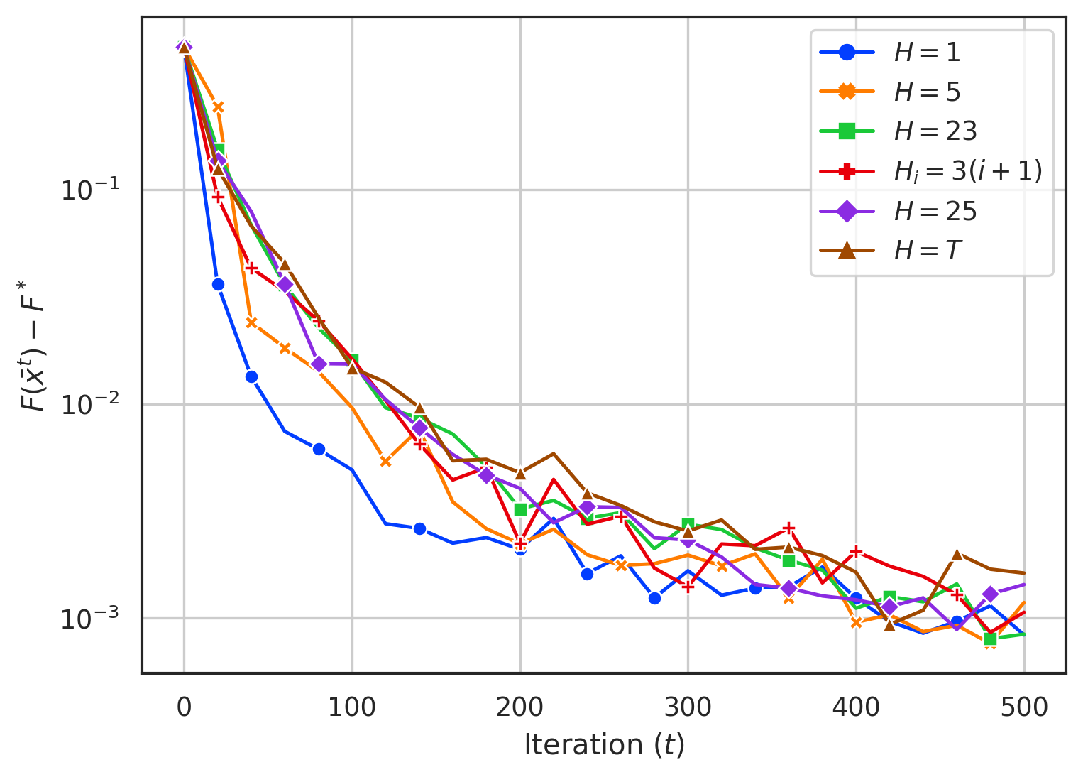
(a) Error over iterations.

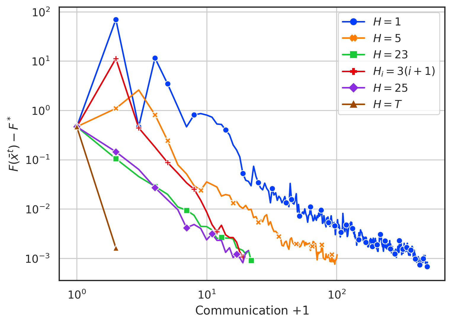
(b) Error over communication rounds.

Figure 2: Local SGD with different communication strategies on the NSQIP data set.

It can be seen that all four communication strategies have similar behavior over the number of iterations. However, the methods proposed in this paper reach the same error level with much less communication rounds, i.e., $20$ versus $143$ ([HKMC19]) or $28$([Sti19]). Surprisingly, one-shot averaging performs just as well as synchronized SGD. This could be due to the fact that our bounds analyze the worst-case scenario. Studying one-shot averaging and cases where it performs well is out of the scope of this paper and is left to future work.

We also notice that, as we get closer to the end of training, the methods with fixed-length communication intervals, have smaller improvement with each communication (see Figure 2-b). However, with the growing communication interval suggested in this paper, each communication decreases the error significantly. This further confirms that less frequent communication is needed towards the end of training.

B.2 Logistic Regression on a9a Data Set

Here we repeat the experiment above on the a9a data set from LIBSVM [CL11]. This data set consists of $N=32561$ data points for training with $d=123$ features. We use same parameters as we did for (NSQIP) data set, except this time we repeat each training $50$ times due to smaller size of the data set. The results are presented in Figure 3. Here, we observe a similar performance of different communication strategies.

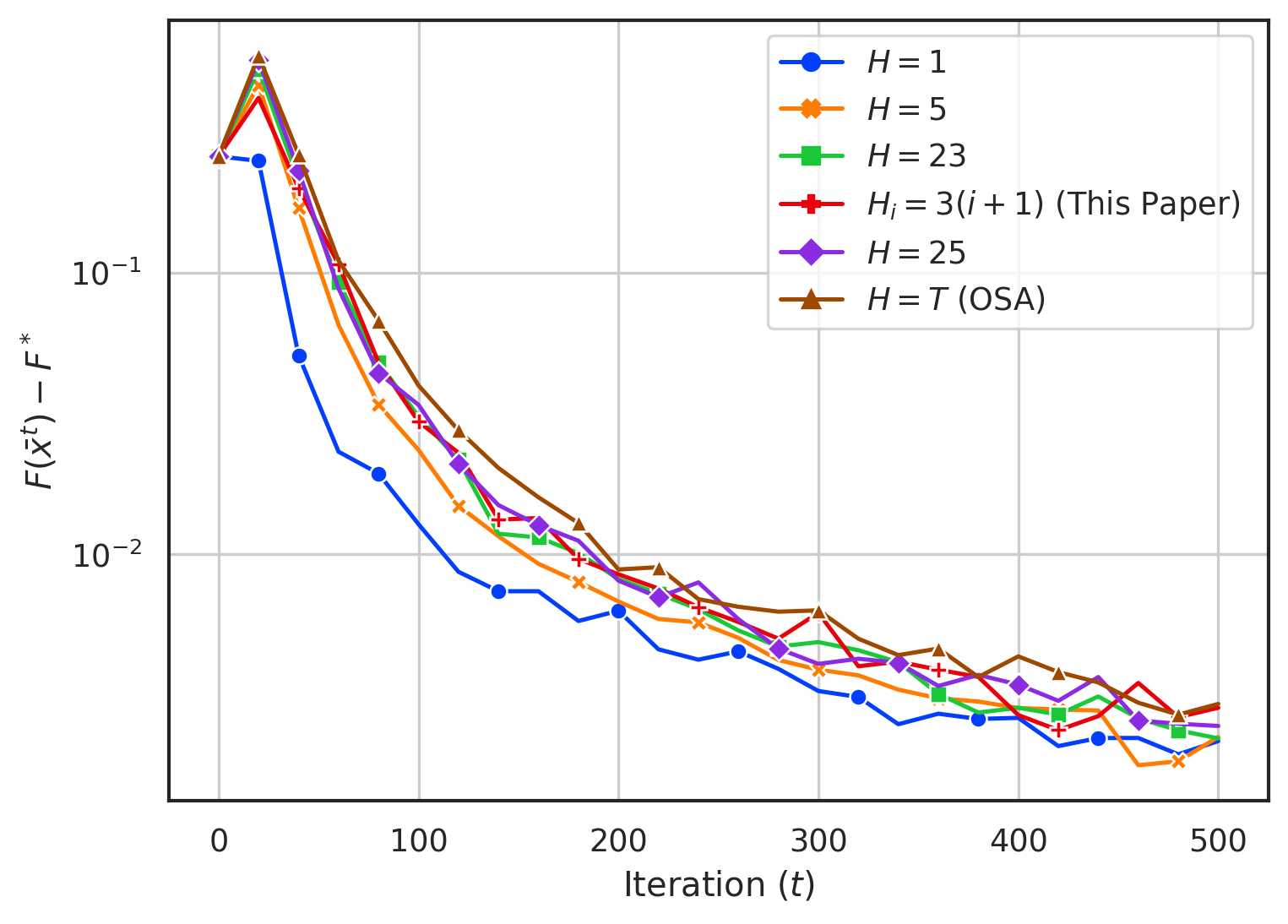
(a) Error over iterations.

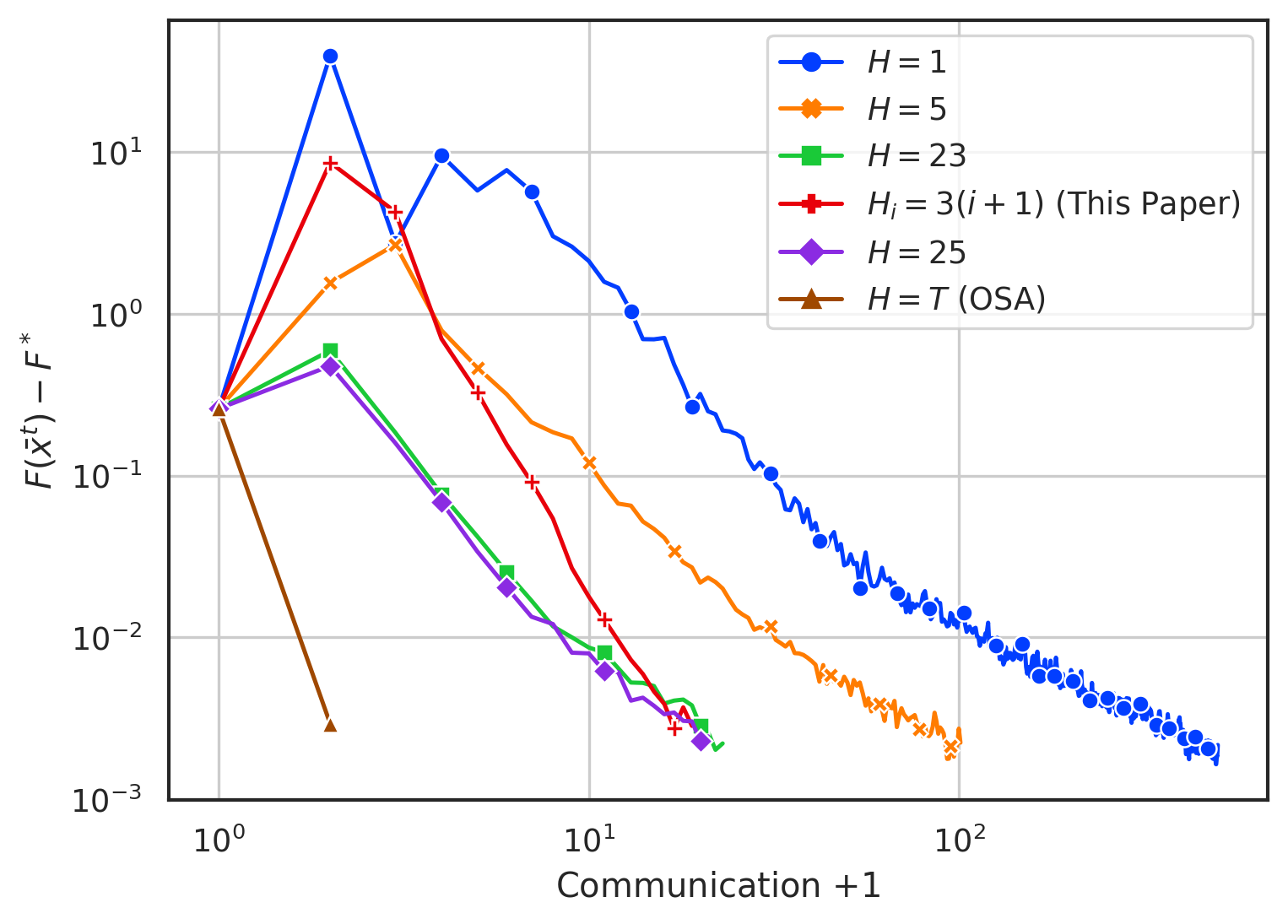
(b) Error over communication rounds.

Figure 3: Local SGD with different communication strategies on the a9a data set.

B.3 Discussion

We note that other communication strategies proposed in related works have often suggested their own step-size sequence or sometimes a fixed step-size. Designing an experiment to have a completely fair comparison of different methods while capturing all possible applications is not easy, if possible at all. Therefore, to make our comparison more fair, we used the same step-size sequence with $\beta=1$ for all methods in each experiment. Moreover, the central goal of the numerical experiments here, is to demonstrate the effectiveness of our suggested communication strategy, using minimal number of communication rounds.

References

- [AGL+17] Dan Alistarh, Demjan Grubic, Jerry Li, Ryota Tomioka, and Milan Vojnovic. Qsgd: Communication-efficient sgd via gradient quantization and encoding. In Advances in Neural Information Processing Systems, pages 1709–1720, 2017.
- [AS15] Yossi Arjevani and Ohad Shamir. Communication complexity of distributed convex learning and optimization. In Advances in neural information processing systems, pages 1756–1764, 2015.
- [BSS16] Avleen S Bijral, Anand D Sarwate, and Nathan Srebro. On data dependence in distributed stochastic optimization. arXiv preprint arXiv:1603.04379, 2016.
- [CL11] Chih-Chung Chang and Chih-Jen Lin. LIBSVM: A library for support vector machines. ACM Transactions on Intelligent Systems and Technology, 2:27:1–27:27, 2011. Software available at http://www.csie.ntu.edu.tw/~cjlin/libsvm.
- [DGBSX12] Ofer Dekel, Ran Gilad-Bachrach, Ohad Shamir, and Lin Xiao. Optimal distributed online prediction using mini-batches. Journal of Machine Learning Research, 13(Jan):165–202, 2012.
- [DP19] Aymeric Dieuleveut and Kumar Kshitij Patel. Communication trade-offs for local-sgd with large step size. In Advances in Neural Information Processing Systems, pages 13579–13590, 2019.
- [GBS20] Antoine Godichon-Baggioni and Sofiane Saadane. On the rates of convergence of parallelized averaged stochastic gradient algorithms. Statistics, pages 1–18, 2020.
- [HBM19] Hadrien Hendrikx, Francis Bach, and Laurent Massoulié. An accelerated decentralized stochastic proximal algorithm for finite sums. In Advances in Neural Information Processing Systems, pages 952–962, 2019.
- [HKMC19] Farzin Haddadpour, Mohammad Mahdi Kamani, Mehrdad Mahdavi, and Viveck Cadambe. Local sgd with periodic averaging: Tighter analysis and adaptive synchronization. In Advances in Neural Information Processing Systems, pages 11080–11092, 2019.
- [KLB+20] Anastasia Koloskova, Nicolas Loizou, Sadra Boreiri, Martin Jaggi, and Sebastian U Stich. A unified theory of decentralized sgd with changing topology and local updates. arXiv preprint arXiv:2003.10422, 2020.
- [KMA+19] Peter Kairouz, H Brendan McMahan, Brendan Avent, Aurélien Bellet, Mehdi Bennis, Arjun Nitin Bhagoji, Keith Bonawitz, Zachary Charles, Graham Cormode, Rachel Cummings, et al. Advances and open problems in federated learning. arXiv preprint arXiv:1912.04977, 2019.
- [KMR20] A Khaled, K Mishchenko, and P Richtárik. Tighter theory for local sgd on identical and heterogeneous data. In The 23rd International Conference on Artificial Intelligence and Statistics (AISTATS 2020), 2020.
- [KMY+16] Jakub Konečnỳ, H Brendan McMahan, Felix X Yu, Peter Richtárik, Ananda Theertha Suresh, and Dave Bacon. Federated learning: Strategies for improving communication efficiency. arXiv preprint arXiv:1610.05492, 2016.
- [LHM+18] Yujun Lin, Song Han, Huizi Mao, Yu Wang, and Bill Dally. Deep gradient compression: Reducing the communication bandwidth for distributed training. In International Conference on Learning Representations, 2018.
- [LSPJ18] Tao Lin, Sebastian U Stich, Kumar Kshitij Patel, and Martin Jaggi. Don’t use large mini-batches, use local sgd. arXiv preprint arXiv:1808.07217, 2018.
- [MHM10] Ryan McDonald, Keith Hall, and Gideon Mann. Distributed training strategies for the structured perceptron. In Human language technologies: The 2010 annual conference of the North American chapter of the association for computational linguistics, pages 456–464. Association for Computational Linguistics, 2010.
- [MMR+17] Brendan McMahan, Eider Moore, Daniel Ramage, Seth Hampson, and Blaise Aguera y Arcas. Communication-efficient learning of deep networks from decentralized data. In Artificial Intelligence and Statistics, pages 1273–1282, 2017.
- [MMS+09] Ryan Mcdonald, Mehryar Mohri, Nathan Silberman, Dan Walker, and Gideon S Mann. Efficient large-scale distributed training of conditional maximum entropy models. In Advances in neural information processing systems, pages 1231–1239, 2009.
- [RN16] Jonathan D Rosenblatt and Boaz Nadler. On the optimality of averaging in distributed statistical learning. Information and Inference: A Journal of the IMA, 5(4):379–404, 2016.
- [SCJ18] Sebastian U Stich, Jean-Baptiste Cordonnier, and Martin Jaggi. Sparsified sgd with memory. In Advances in Neural Information Processing Systems, pages 4447–4458, 2018.
- [SK19] Sebastian U Stich and Sai Praneeth Karimireddy. The error-feedback framework: Better rates for sgd with delayed gradients and compressed communication. arXiv preprint arXiv:1909.05350, 2019.
- [SOP20] Artin Spiridonoff, Alex Olshevsky, and Ioannis Ch Paschalidis. Robust asynchronous stochastic gradient-push: asymptotically optimal and network-independent performance for strongly convex functions. Journal of Machine Learning Research, 2020.
- [SR13] Mark Schmidt and Nicolas Le Roux. Fast convergence of stochastic gradient descent under a strong growth condition. arXiv preprint arXiv:1308.6370, 2013.
- [Sti19] Sebastian U. Stich. Local SGD converges fast and communicates little. In International Conference on Learning Representations, 2019.
- [TSC+20] Zhenheng Tang, Shaohuai Shi, Xiaowen Chu, Wei Wang, and Bo Li. Communication-efficient distributed deep learning: A comprehensive survey. arXiv preprint arXiv:2003.06307, 2020.
- [WJ18a] Jianyu Wang and Gauri Joshi. Adaptive communication strategies to achieve the best error-runtime trade-off in local-update sgd. Systems for ML, 2018.
- [WJ18b] Jianyu Wang and Gauri Joshi. Cooperative sgd: A unified framework for the design and analysis of communication-efficient sgd algorithms. arXiv preprint arXiv:1808.07576, 2018.
- [WPS+20] Blake Woodworth, Kumar Kshitij Patel, Sebastian U Stich, Zhen Dai, Brian Bullins, H Brendan McMahan, Ohad Shamir, and Nathan Srebro. Is local sgd better than minibatch sgd? arXiv preprint arXiv:2002.07839, 2020.
- [WSY+19] Jianyu Wang, Anit Kumar Sahu, Zhouyi Yang, Gauri Joshi, and Soummya Kar. Matcha: Speeding up decentralized sgd via matching decomposition sampling. arXiv preprint arXiv:1905.09435, 2019.
- [WWLZ18] Jianqiao Wangni, Jialei Wang, Ji Liu, and Tong Zhang. Gradient sparsification for communication-efficient distributed optimization. In Advances in Neural Information Processing Systems, pages 1299–1309, 2018.
- [YYZ19] Hao Yu, Sen Yang, and Shenghuo Zhu. Parallel restarted sgd with faster convergence and less communication: Demystifying why model averaging works for deep learning. In Proceedings of the AAAI Conference on Artificial Intelligence, volume 33, pages 5693–5700, 2019.
- [ZC18] Fan Zhou and Guojing Cong. On the convergence properties of a k-step averaging stochastic gradient descent algorithm for nonconvex optimization. In Proceedings of the 27th International Joint Conference on Artificial Intelligence, pages 3219–3227. AAAI Press, 2018.
- [ZCL15] Sixin Zhang, Anna E Choromanska, and Yann LeCun. Deep learning with elastic averaging sgd. In Advances in neural information processing systems, pages 685–693, 2015.
- [ZDJW13] Yuchen Zhang, John Duchi, Michael I Jordan, and Martin J Wainwright. Information-theoretic lower bounds for distributed statistical estimation with communication constraints. In Advances in Neural Information Processing Systems, pages 2328–2336, 2013.
- [ZDSMR16] Jian Zhang, Christopher De Sa, Ioannis Mitliagkas, and Christopher Ré. Parallel sgd: When does averaging help? arXiv preprint arXiv:1606.07365, 2016.
- [ZDW13] Yuchen Zhang, John C Duchi, and Martin J Wainwright. Communication-efficient algorithms for statistical optimization. Journal of Machine Learning Research, 14(1):3321–3363, 2013.
- [ZWLS10] Martin Zinkevich, Markus Weimer, Lihong Li, and Alex J Smola. Parallelized stochastic gradient descent. In Advances in neural information processing systems, pages 2595–2603, 2010.