Suppression of the quasi-two-dimensional quantum collapse in the attraction field by the Lee-Huang-Yang effect

Abstract

Quantum collapse in three and two dimensions (3D and 2D) is induced by attractive potential $\sim-r^{-2}$. It was demonstrated that the mean-field (MF) cubic self-repulsion in the 3D bosonic gas suppresses the collapse and creates the missing ground state (GS). However, the cubic nonlinearity is not strong enough to suppress the 2D collapse. We demonstrate that the Lee-Hung-Yang (LHY) quartic term, induced by quantum fluctuations around the MF state, is sufficient for the stabilization of the 2D gas against the collapse. By means of numerical solution of the Gross-Pitaevskii equation including the LHY term, as well as with the help of analytical methods, such as expansions of the wave function at small and large distances from the center and the Thomas-Fermi approximation, we construct stable GS, with a singular density, $\sim r^{-4/3}$ but convergent integral norm. Counter-intuitively, the stable GS exists even if the external potential is repulsive, with the strength falling below a certain critical value. An explanation to this finding is given. Along with the GS, singular vortex states are produced too, and their stability boundary is found analytically. Unstable vortices spontaneously transform into the stable GS, expelling the vorticity to periphery.

I Introduction and the model

The quantum collapse, alias “fall onto the center” LL , is a well-known phenomenon in quantum mechanics: nonexistence of the ground state (GS) in three- and two-dimensional (3D and 2D) Schrödinger equations with attractive potential

$$U(r)=-\left(U_{0}/2\right)r^{-2},$$ (1)

where $r$ is the radial coordinate, and positive $U_{0}$ is the strength of the pull to the center. Note that, under the action of potential (1), classical particle of mass $M$ performs motion with angular frequency

$$\omega=\sqrt{U_{0}/M}r^{-2}$$ (2)

along a circular orbit with arbitrary radius $r$.

In 3D, the collapse occurs when $U_{0}$ exceeds a finite critical value [$\left(U_{0}\right)_{\mathrm{coll}}=1/4$ in the notation adopted below], while in two dimensions $\left(U_{0}\right)_{\mathrm{coll}}=0$, i.e., the 2D collapse happens at any $U_{0}>0$. In both 3D and 2D cases, the potential represents attraction of a particle (small molecule), carrying a permanent electric dipole moment, to a central charge, assuming that the local orientation of the dipole is fixed by the minimization of its energy in the external field HS1 . In addition to that, in the 2D case the same potential (1) may be realized as the attraction of a magnetically polarizable atom to a thread carrying electric current (e.g., an electron beam) transversely to the system’s plane, or the attraction of an electrically polarizable atom to a uniformly charged transverse thread. Other 2D settings in Bose-Einstein condensates (BECs) under the action of similar fields were considered in Refs. Austria1 and Austria2 .

A fundamental issue is regularization of the setting, aiming to create a missing GS. One solution was proposed in Refs. QTF1 -QTF3 , which replaced the original quantum-mechanical problem by one based on a linear quantum field theory. A solution of the latter model produces a GS, but it does not answer a natural question, what the size of the GS is for given parameters of the setting, such as $U_{0}$ and mass of the quantum particle, $M$. In fact, the solution defines the GS size as an arbitrary spatial scale, which varies as a parameter of the respective quantum-field renormalization group.

Another solution was proposed in Ref. HS1 , replacing the 3D linear Schrödinger equation by the Gross-Pitaevskii (GP) equation GP for a gas of the dipole particles pulled to the center by Coulomb potential (1), and stabilized by repulsive inter-particle interactions. Further, in the mean-field (MF) approximation which, in particular, assumes the interaction of the dipole moment of each particle with the electrostatic field created, as per the Poisson equation, by all other dipoles, the dipole-dipole interactions between the particles amount to an extra local cubic term, added to the contact repulsive interaction HS1 . As a results, it was found that, in the framework of the MF approximation, the three-dimensional GP equation creates the missing GS for arbitrarily large $U_{0}$. The size of this GS is fully determined by parameters of the physical system ($U_{0}$, $M$, the scattering length of the inter-particle interactions, and the number of particles, $N$), being $\sim$ a few $\mathrm{\mu}$m for typical values of the physical parameters. Furthermore, beyond the bounds of the MF consideration, it was demonstrated that, in terms of the many-body quantum theory, treated by means of the variational Monte-Carlo method, the GS, strictly speaking, does not exist in the same setting (the collapse is still possible), but the interplay of the pull to the center and inter-particle repulsion gives rise to a metastable state, which, for a sufficiently large $N$, is virtually tantamount to the GS, being separated from the collapsing state by a tall potential barrier Gregory . Subsequently, the mean-field GS was also found in the 3D gas of dipole molecules embedded in a strong uniform electric field, which reduces the underlying symmetry from spherical to cylindrical HS2 , and in the two-component 3D gas HS3 , see also a brief review in Ref. cond-matter .

The situation is more problematic in 2D, as the usual self-defocusing cubic nonlinearity, which represents the two-body inter-atomic repulsion in the MF approximation GP , is not strong enough to suppress the collapse and create the GS. The problem is that the MF wave function, $\Psi(r)$, produced by the respective GP equation, gives rise to the density, $\left|\Psi(r)\right|^{2}$, diverging $\sim r^{-2}$ at $r\rightarrow 0$, in 3D and 2D alike, as this form of the solution is supported by the balance between the kinetic-energy, pulling-potential, and cubic terms in the GP equation. Then, in terms of the integral norm,

$$N=\left(2\pi\right)^{D-1}\int_{0}^{\infty}\left|\Psi(r)\right|^{2}r^{D-1}dr,$$ (3)

where $D=3$ or $2$ is the dimension, the density singularity $\sim r^{-2}$ is integrable in 3D, while it gives rise to a logarithmic divergence in 2D:

$$N\sim\ln\left(r_{\mathrm{cutoff}}^{-1}\right),$$ (4)

where $r_{\mathrm{cutoff}}$ is the cutoff (smallest) radius. The analysis of the GP equation readily demonstrates that a self-repulsive nonlinear term stronger than cubic, i.e., $|\Psi|^{\alpha-1}\Psi$ with $\alpha>3$, gives rise to the asymptotic form of the density

$$|\Psi(r)|^{2}\sim r^{-4/(\alpha-1)}.$$ (5)

Thus, any value $\alpha>3$ provides convergence of the 2D integral norm, given by Eq. (3) with $D=2$. In 3D, Eqs. (5) and (3) demonstrate that the critical value of the repulsive-nonlinearity power, which also entails the logarithmic divergence [cf. Eq. (4)], is $\alpha=7/3$ (it is relevant to mention that $\alpha=7/3$ corresponds to the effective repulsion in the density-functional model of the Fermi gas Fermi2 -Fermi3 ).

Thus, a solution for the regularization of the 2D setting may be offered by the quintic defocusing nonlinearity HS1 , with $\alpha=5$. The quintic term accounts for three-body repulsive interactions in the bosonic gas Abdullaev1 ; Abdullaev2 , although an essential difficulty in the physical realization of the latter feature is the fact that three-particle collisions give rise to effective losses, by kicking out particles from BEC to the thermal halo loss1 -loss3 .

Recently, much interest was drawn to the formation of quasi-2D and 3D self-trapped states in BEC in the form of “quantum droplets”, filled by an effectively incompressible binary condensate, which is considered as an ultradilute quantum fluid. This possibility was predicted in the framework of the 3D Petrov and 2D Petrov-Astra ; Zin ; Santos GP equations which include the Lee-Huang-Yang (LHY) corrections to the MF approximation, that represent effects of quantum fluctuations around the MF states LHY . The binary structure of the underlying condensate is essential because the nearly complete cancellation between the inter-component MF attraction and intra-component repulsion (which may be adjusted by means of the Feshbach-resonance technique Feshbach ) makes it possible to create stable droplets through the balance of the LHY-induced higher-order (quartic) self-repulsion and the relatively weak residual MF attraction, accounted for by the cubic term. The so predicted quantum droplets were created with quasi-2D (oblate) Leticia1 ; Leticia2 and fully 3D (isotropic) Inguscio1 ; Inguscio2 shapes in a mixture of two different spin states of ³⁹K atoms, as well as in a heteronuclear mixture of ⁴¹K and ⁸⁷Rb atoms hetero . Further, it was theoretically predicted that 2D Raymond1 ; Raymond2 ; lattice and 3D Barcelona droplets with embedded vorticity have their well-defined stability regions too. The LHY effect also helps to create stable 3D droplets in single-component BECs with long-range interactions between atoms carrying magnetic dipole moments, as was demonstrated experimentally and studied in detail theoretically Pfau1 -Pfau5 , although dipolar-condensate droplets carrying embedded vorticity are unstable Macri .

The objective of the present work is to make use of the LHY effect for the stabilization of the GS in the quasi-2D bosonic gas pulled to the center by potential (1). This possibility is essential because, as said above, the alternative, in the form of the quintic self-repulsion, is problematic in the real BEC setting. The underlying full (3D) GP equation, including the LHY-induced quartic defocusing term, is written in physical units as Petrov

$$i\hbar\frac{\partial\Psi}{\partial t}=-\frac{\hbar^{2}}{2M}\nabla^{2}\Psi+V(\mathbf{r})\Psi+\frac{4\pi\hbar^{2}\delta a}{M}|\Psi|^{2}\Psi+\frac{256\sqrt{2\pi}\hbar^{2}}{3M}a^{5/2}|\Psi|^{3}\Psi,$$ (6)

where $\Psi$ represents equal wave functions of two components of the binary BEC, $V(\mathbf{r})$ is the general trapping potential, $a>0$ is the scattering length of inter-particle collisions, which induce the cubic MF self-repulsion in each component, $\delta a\gtrless 0$, with $\left|\delta a\right|\ll a$, represents the small disbalance of the inter-component attraction and intra-component repulsion, the last term in Eq. (6) being the LHY correction to the MF equation. It is relevant to mention that, in principle, the same equation, with $\delta a$ replaced by $a$, is valid for a single-component self-repulsive BEC. However, without the nearly full cancellation of the MF interactions, the LHY correction is negligibly weak, therefore it will not provide the efficient stabilization sought for.

The reduction of Eq. (6) to the 2D form, with coordinates $\left(x,y\right)$, under the action of extremely tight confinement applied in the $z$ direction, was elaborated in Ref. Petrov-Astra , leading to an effective cubic nonlinearity with an extra logarithmic factor,

$$\left(\mathrm{nonlin}\right)_{\mathrm{2D}}\sim|\Psi|^{2}\ln\left(|\Psi|^{2}/\Psi_{0}^{2}\right)\Psi,$$ (7)

which is attractive and repulsive at $|\Psi|^{2}<\Psi_{0}^{2}$ and $|\Psi|^{2}>\Psi_{0}^{2}$, respectively, where $\Psi_{0}^{2}$ corresponds to the density determined by the equilibrium between the MF and LHY interactions, that, in physical units, is $n_{0}=\left(25\pi/2^{15}\right)\left(\delta a/a\right)^{2}a^{-3}$ Petrov . However, this limit case corresponds to extremely strong confinement in the $z$ direction, with the transverse size $a_{\perp}\ll\xi$, where the healing length, corresponding to the equilibrium density, is estimated as $\xi=\left(32\sqrt{2}/3\pi\right)\left(a/\left|\delta a\right|\right)^{3/2}a\approx 5\left(a/\left|\delta a\right|\right)^{3/2}a$. Then, typical experimentally relevant parameters Leticia1 -Inguscio2 yield $\xi\simeq 30$ nm. On the other hand, an experimentally relevant transverse-confinement length is $a_{\perp}\sim 0.6$ $\mathrm{\mu}$m Leticia1 , implying relation $a_{\perp}\gg\xi$, which is opposite to the above-mentioned necessary one. Thus, it is relevant to reduce Eq. (6) to the 2D form, keeping the same nonlinearity as in Eq. (6). In this connection, we note that, as straightforward analysis demonstrates, the modified nonlinear term (7), corresponding to the ultra-tight confinement, is insufficient to create a GS with a convergent norm in 2D, yielding the density singularity $\left|\Psi\right|^{2}\sim r^{-2}/\ln\left(r^{-1}\right)$ at $r\rightarrow 0$, hence the two-dimensional integral (3) is still diverging, although extremely slowly: $N\sim\ln\left(\ln\left(r_{\mathrm{cutoff}}^{-1}\right)\right)$, cf. Eq. (4). On the other hand, the reduction of the full 3D problem to the 2D approximation is relevant as long as the radial size of the resulting bound state, $R$, exceeds $a_{\perp}$ by an order of magnitude (or greater). It is expected that the predicted stable states will have $R\sim 10$ $\mathrm{\mu}$m (see below), which justifies the latter assumption.

To complete the derivation of the effective 2D equation, we first rescale three-dimensional Eq. (6), measuring the density, length, time, and the trapping potential, respectively, in units of $\left(36/25\right)n_{0}$, $\xi$, $\tau\equiv\left(M/\hbar\right)\xi^{2}$, and $\hbar/\tau$:

$$i\frac{\partial\Psi}{\partial t}=-\frac{1}{2}\nabla^{2}\Psi+\sigma|\Psi|^{2}\Psi+|\Psi|^{3}\Psi+V(\mathbf{r})\Psi,$$ (8)

where $\sigma=\pm 1$ is the sign of $\delta a$, the potential is a sum of the above-mentioned term (1) and the transverse-confinement one, $\left(1/2\right)a_{\perp}^{-4}z^{2}$. In this notation, the above-mentioned critical strength of the pulling potential in the linearized version of the 3D equation (8) is $\left(U_{0}\right)_{\mathrm{coll}}=1/4$. Then, the 3D $\rightarrow$ 2D reduction is performed by means of the standard substitution Luca ; Delgado , $\Psi\left(x,y,z,t\right)=\psi\left(x,y,t\right)\exp\left(-z^{2}/2a_{\perp}^{2}\right)$, followed by the averaging of Eq. (8) in the transverse direction. Finally, with the help of additional rescaling, $\psi\rightarrow\left(2/\sqrt{5}\right)\psi$, $\left(x,y\right)\rightarrow\left(\sqrt{5}/2\right)\left(x,y\right)$, and $t\rightarrow\left(5/4\right)t$, the effective two-dimensional GP equation, written in terms of the polar coordinates $\left(r,\theta\right)$ in the $\left(x,y\right)$ plane, is cast in the form of

$$i\frac{\partial\psi}{\partial t}=-\frac{1}{2}\left(\frac{\partial^{2}\psi}{\partial r^{2}}+\frac{1}{r}\frac{\partial\psi}{\partial r}+\frac{1}{r^{2}}\frac{\partial^{2}\psi}{\partial\theta^{2}}\right)-\frac{U_{0}}{2r^{2}}\psi+\sigma\left|\psi\right|^{2}\psi+|\psi|^{3}\psi,$$ (9)

which includes the pulling-to-the-center potential (1). This equation conserves, along with norm

$$N=\int\int\left|\psi\left(x,y\right)\right|^{2}dxdy,$$ (10)

cf. Eq. (3), the Hamiltonian,

$$H=\int\int\left[\frac{1}{2}\left(\left|\nabla\psi\right|^{2}-\frac{U_{0}}{r^{2}}\left|\psi\right|^{2}+\sigma\left|\psi\right|^{4}\right)+\frac{2}{5}\left|\psi\right|^{5}\right]dxdy,$$ (11)

and the angular momentum,

$$L_{z}=i\int\int\frac{\partial\psi^{\ast}}{\partial\theta}\psi dxdy,$$ (12)

where $\ast$ stands for the complex conjugation.

It is also relevant to consider the case when the balance between the inter-component attraction and intra-component repulsion makes it possible to set $\delta a=0$, the entire nonlinearity originating from the LHY term, cf. Ref. LHY-only . The respective 2D equation (produced by an obviously different rescaling) takes the form of Eq. (9) with $\sigma=0$. In fact, this case is the most fundamental one, as the suppression of the 2D collapse and formation of the GS is provided by the quartic term, while, in any case, the cubic term plays a minor role.

The rest of the paper is organized as follows. In Section II we produce analytical results, which are based on the asymptotic consideration of Eq. (9) for stationary solutions in the form of the GS and vortex states, as well as for small perturbations which determine their stability. Analytical considerations also make use of the Thomas-Fermi (TF) approximation, which produces accurate results in the case of $\sigma=0$. Numerical findings, produced by systematic simulations of Eq. (9), are summarized in Section III. They demonstrate that the zero-vorticity states are completely stable, in agreement with the conjecture that they represent the system’s GS, while the vortical modes feature an instability boundary (which is predicted in an exact analytical form in Section II). Unstable vortices (roughly speaking, those existing in the case of relatively small $U_{0}$) spontaneously develop spiral motion of the vortex’ pivot from the center to periphery, which eventually leads to replacement of the unstable vortex by the stable GS. A counterintuitive finding is that the stable zero-vorticity GS can be found even in the interval of $-4/9<U_{0}<0$, where the central potential is (weakly) repulsive. An explanation of this fact is given too. The paper is concluded by Section IV.

II Analytical considerations

II.1 Asymptotic forms of the solutions

Stationary solutions to Eq. (9) with chemical potential $\mu$ and integer vorticity (orbital quantum number) $l=0,1,2,...$, are looked for as

$$\psi\left(r,t\right)=\exp\left(-i\mu t+il\theta\right)u(r),$$ (13)

with real radial function satisfying the equation

$$\mu u=-\frac{1}{2}\left(\frac{d^{2}u}{dr^{2}}+\frac{1}{r}\frac{du}{dr}+\frac{U_{l}}{r^{2}}u\right)+\sigma u^{3}+u^{4},$$ (14)

where we define

$$U_{l}\equiv U_{0}-l^{2}.$$ (15)

The asymptotic form of the solution to Eq. (14) at $r\rightarrow 0$ is

$$u=\left[\frac{1}{2}\left(U_{l}+\frac{4}{9}\right)\right]^{1/3}r^{-2/3}-\sigma\frac{9U_{l}+4}{27U_{l}+16}+O\left(r^{2/3}\right).$$ (16)

The singularity of the asymptotic solution (16), $\sim r^{-2/3}$, with the power which is determined by the balance between the LHY quartic term and the attractive potential, and does not depend on $l$ and $\sigma$, is weak enough to secure the convergence of the integral norm (3) at $r\rightarrow 0$. It is worthy to note that, as seen in Eq. (16), the expansion of the solution at $r\rightarrow 0$ is performed in powers of $r^{2/3}$.

Obviously, solutions to Eq. (14) may be localized at $r\rightarrow\infty$ for $\mu<0$. Then, in the case of $\sigma=0$, a simple corollary of Eq. (14) is an exact scaling relation which shows the dependence of the solution on $|\mu|$:

$$u\left(r;\mu\right)=\left|\mu\right|^{1/3}u\left(|\mu|^{-1/2}r;\mu=-1\right).$$ (17)

Further, the substitution of this expression in Eq. (3) yields an exact scaling relation for the norm of the 2D state, at $\sigma=0$:

$$N(\mu)=|\mu|^{-1/3}N(\mu=-1).$$ (18)

We note that this relation satisfies the anti-Vakhitov-Kolokolov (VK) criterion, $dN/d\mu>0$, which was proposed as a necessary stability condition for trapped modes supported by the defocusing nonlinearity anti (the VK criterion proper states that $dN/d\mu<0$ is necessary for the stability of self-trapped modes in the case of focusing nonlinearity VK ; Berge ). Below, we demonstrate that the GS family is completely stable in the present model.

Asymptotic expression (16) suggests substitution

$$\psi\left(r,\theta,t\right)\equiv r^{-2/3}\varphi\left(r,\theta,t\right),u(r)\equiv r^{-2/3}\chi(r),$$ (19)

which transforms Eqs. (9) and (14) into

$$i\frac{\partial\varphi}{\partial t} = -\frac{1}{2}\left[\frac{\partial^{2}}{\partial r^{2}}-\frac{1}{3r}\frac{\partial}{\partial r}+\frac{\left(U_{0}+4/9\right)}{r^{2}}+\frac{1}{r^{2}}\frac{\partial^{2}}{\partial\theta^{2}}\right]\varphi$$ (20)

$$+\sigma\frac{|\varphi|^{2}\varphi}{r^{4/3}}+\frac{|\varphi|^{3}\varphi}{r^{2}},$$

$$\mu\chi=-\frac{1}{2}\left[\frac{d^{2}\chi}{dr^{2}}-\frac{1}{3r}\frac{d\chi}{dr}+\frac{\left(U_{l}+4/9\right)}{r^{2}}\chi\right]+\sigma\frac{\chi^{3}}{r^{4/3}}+\frac{\chi^{4}}{r^{2}}.$$ (21)

Accordingly, the asymptotic form (21) of the solution at $r\rightarrow 0$ is replaced by a singularity-free expansion,

$$\chi(r;U_{l},\sigma)=\left[\frac{1}{2}\left(U_{l}+\frac{4}{9}\right)\right]^{1/3}-\sigma\frac{9U_{l}+4}{27U_{l}+16}r^{2/3}+O\left(r^{4/3}\right).$$ (22)

The first correction to the leading term in this expansion vanishes in the case of $\sigma=0$ (no MF nonlinearity). Then, it follows from Eq. (21) that the expansion is replaced by

$$\chi(r;U_{l},\sigma=0)=\left[\frac{1}{2}\left(U_{l}+\frac{4}{9}\right)\right]^{1/3}\left(1+\frac{2\mu}{3U_{l}}r^{2}\right)+O\left(r^{4}\right),$$ (23)

which is valid for $U_{l}>0$. In the interval of

$$-4/9<U_{l}<0$$ (24)

(the meaning of this interval is explained below), the quadratic term in Eq. (23) is valid too, but in that case it is not a leading correction, as Eq. (22) admits a stronger one, $\mathrm{const}\cdot r^{\beta}$, with $\beta=2/3+\sqrt{16/9+3U_{l}}<2$, while $\mathrm{const}$ remains indefinite, in terms of the expansion at $r\rightarrow 0$. Exactly at $U_{l}=0$, Eq. (23) is replaced by

$$\chi(r;U_{l}=\sigma=0)=\left(\frac{2}{9}\right)^{1/3}\left(1+\frac{3\mu}{4}r^{2}\ln\left(\frac{r_{0}}{r}\right)\right)+~{}...,$$ (25)

where constant $r_{0}$ is also indefinite.

The asymptotic form of the solution, given by Eq. (22), is meaningful if it yields $u(r)>0$ [otherwise, the derivation of Eq. (14) from Eq. (9) is irrelevant], i.e., for $U_{l}>0$, as well as for weakly negative values of the effective strength of the central potential belonging to interval (24), which implies

$$l^{2}-4/9<U_{0}\leq l^{2}.$$ (26)

For the vortex states, with $l\geq 1$, condition (26) means, in any case, $U_{0}>0$, but for the GS, with $l=0$, Eq. (26) admits negative $U_{0}$ with sufficiently small absolute values, viz., $0\leq-U_{0}<4/9$. In the limit of $U_{0}+4/9\rightarrow+0$, further analysis of Eq. (21) yields the following asymptotically exact solution, which does not depend on $\sigma$:

$$\left(\chi(r)\right)_{U_{l}+4/9\rightarrow 0}=\frac{\sqrt{3}\Gamma(1/3)}{\pi}\left[\frac{|\mu|}{4}\left(U_{l}+\frac{4}{9}\right)\right]^{1/3}r^{2/3}K_{2/3}\left(\sqrt{2|\mu|}r\right),$$ (27)

where $\Gamma(1/3)\approx\allowbreak 2.68$ is the value of the Gamma-function, and $K_{2/3}$ is the standard modified Hankel’s function (alias the modified Bessel function of the second kind). The substitution of this expression and one defined by Eq. (19) in Eq. (3) (with $D=2$) yields the respective result for the norm:

$$N_{U_{l}+4/9\rightarrow 0}=\frac{\Gamma^{2}(1/3)}{\sqrt{3}}\frac{\left(U_{l}+4/9\right)^{2/3}}{\left(2|\mu|\right)^{1/3}}.$$ (28)

Note that this result agrees with the general scaling relation (18).

While the existence of the bound state under the combined action of the repulsive potential and dominating defocusing quartic nonlinearity is a counterintuitive finding, it is closely related to the previously known fact that the 2D nonlinear Schrödinger equations with the repulsive nonlinear term $|u|^{p-1}u$ supports localized solutions with a singular asymptotic form,

$$u\approx\left[\frac{1}{2}\left(\frac{4}{\left(p-1\right)^{2}}+U_{0}\right)\right]^{1/\left(p-1\right)}r^{-2/\left(p-1\right)}$$ (29)

at $r\rightarrow 0$ Veron [here, Eq. (29) takes into account the presence of the potential with strength $U_{0}$ in Eq. (14), which was not included in Ref. Veron ]. It is seen that this singular state exists at $0<-U_{0}<4/\left(p-1\right)^{2}$, and the integral which defines its norm converges at $r\rightarrow 0$ for $p>3$, including the case of the quartic nonlinearity, with $p=4$. This result, which was originally obtained as a formal one Veron , may be understood, in terms of the physical realization, as an effect created by an additional delta-functional attractive potential, which is concentrated on a sphere of a vanishingly small radius $\rho$:

$$U_{\delta}=-\lim_{\rho\rightarrow 0}\left[\varepsilon\delta\left(r-\rho\right)\right],~{}\varepsilon\equiv\left(p-1\right)^{-1}\rho^{-1}.$$ (30)

This potential, added to the model, becomes “invisible” in the limit of $\rho\rightarrow 0$ in Eq. (30), being screened by the singular profile of the pinned state HS . This consideration explains the possibility of the existence of the bound state which is not supported by any apparent factor pulling the wave function to the center. Note that the “charge” of the invisible potential, $Q\equiv 2\pi\rho\cdot\varepsilon=2\pi/\left(p-1\right)$, remains finite in the limit of $\delta\rightarrow 0$. In similar 1D and 3D settings, the screened charge is, respectively, diverging or vanishingly small, $Q_{\mathrm{1D}}\sim\rho^{-1}$ and $Q_{\mathrm{3D}}\sim\rho$ HS , see also a brief review of the topic in Ref. we .

In the limit of $r\rightarrow\infty$, the asymptotic form of the solution to Eq. (21) is

$$\chi(r)\approx\chi_{0}r^{1/6}\exp\left(-\sqrt{2|\mu|}r\right),$$ (31)

where $\chi_{0}$ is an arbitrary constant (in terms of the asymptotic form at $r\rightarrow\infty$), and $\mu$ must be negative. An approximate global interpolation for the solution may be produced by combining asymptotic forms (22) and (31):

$$\chi_{\mathrm{interpol}}(r)=\left[\frac{1}{2}\left(U_{l}+\frac{4}{9}\right)\right]^{1/3}\exp\left(-\sqrt{2|\mu|}r\right).$$ (32)

Of course, this is a coarse approximation, as it postulates a wrong power of the pre-exponential factor at $r\rightarrow\infty$ [$0$ instead of $1/6$, see Eq. (31)], and ignores any effect of term $u^{3}$ in Eq. (14). The calculation of norm (3) with the approximate solution given by Eq. (32) produces the respective analytical expression,

$$N_{\mathrm{interpol}}(\mu)=2\pi\int_{0}^{\infty}u_{\mathrm{interpol}}^{2}(r)rdr=\pi\Gamma\left(2/3\right)\frac{\left(U_{l}+4/9\right)^{2/3}}{\left(4|\mu|\right)^{1/3}},$$ (33)

[where $\Gamma(2/3)\approx\allowbreak 1.354$ is the value of the Gamma-function], which also agrees with scaling (18). In the limit of $U_{l}+4/9\rightarrow 0$, the difference between the approximate value of the norm, given by Eq. (33), and the asymptotically exact result (28) amounts to a factor $\approx\allowbreak 0.81$.

II.2 Vortex states and their stability

Usually, the presence of integer vorticity $l\geq 1$ implies that the amplitude vanishes at $r\rightarrow 0$ as $r^{l}$, which is necessary because the phase of the vortex field is not defined at $r=0$. However, the indefiniteness of the phase is also compatible with the amplitude diverging at $r\rightarrow 0$. In the linear equation, this divergence has the asymptotic form of the standard Neumann’s (alias singular Bessel’s) cylindrical function, $Y_{l}(r)\sim r^{-l}$, which makes the respective 2D state unnormalizable (i.e., physically irrelevant) for all values $l\geq 1$. However, in the present system Eq. (16) demonstrates that the interplay of the central potential and quartic nonlinearity reduces the divergence to the level of $r^{-2/3}$, for any $l$, thus maintaining the normalizability of the states under the consideration, similar to what was found in Ref. HS1 , where the quintic repulsive nonlinearity kept the singularity in another form which secured the convergence of the 2D integral norm (3), $u(r)\sim r^{-1/2}$.

Stationary solutions for vortex modes, as produced by Eq. (21), are not essentially different from the GS ones, as the presence of vorticity $l$ affects only the effective potential strength defined by Eq. (15). Real difference between the states with $l=0$ and $l\geq 1$ is revealed by the analysis of their stability. To this end, it is necessary to derive the linearized Bogoliubov - de Gennes (BdG) equations for eigenmodes of small perturbations, with arbitrary integer azimuthal index $m$ and instability growth rate $\lambda$ (which may be complex), added to the stationary states. It is natural to perform this analysis in terms of Eq. (20), which makes it possible to eliminate the singular factor, $r^{-2/3}$, from the perturbations. Thus, the perturbed solution is looked for in the usual form Yang ,

$$\varphi(r,\theta,t)=\exp\left(-i\mu t+il\theta\right)$$

$$\times\left[\chi(r)+v_{1}(r)\exp\left(\lambda t+im\theta\right)+v_{2}^{\ast}(r)\exp\left(\lambda^{\ast}t-im\theta\right)\right],$$ (34)

where $\chi(r)$ is a solution of Eq. (21). The substitution of this in Eq. (9) and linearization with respect to perturbation amplitudes $v_{1,2}$ leads to BdG equations in the radial form:

$$i\lambda v_{1} = -\frac{1}{2}\left[\frac{d^{2}}{dr^{2}}-\frac{1}{3r}\frac{d}{dr}+\frac{U_{0}-(l+m)^{2}+4/9}{r^{2}}\right]v_{1}$$

$$+\sigma\frac{\chi_{0}^{2}}{r^{4/3}}(2v_{1}+v_{2})+\frac{\chi_{0}^{3}}{2r^{2}}(5v_{1}+3v_{2}),$$

$$-i\lambda v_{2} = -\frac{1}{2}\left[\frac{d^{2}}{dr^{2}}-\frac{1}{3r}\frac{d}{dr}+\frac{U_{0}-(l-m)^{2}+4/9}{r^{2}}\right]v_{2}$$ (35)

$$+\sigma\frac{\chi_{0}^{2}}{r^{4/3}}(2v_{2}+v_{1})+\frac{\chi_{0}^{3}}{2r^{2}}(5v_{2}+3v_{1}).$$

The instability driven by the perturbation eigenmode with $m\geq 2$ splits the vortex in $m$ fragments, while the eigenmode with $m=1$ is a dipole perturbation which drives spontaneous drift of the vortex’ pivot from the original position old-review . By solving the eigenvalue problem based on Eq. (35), one can find the spectrum of instability growth rates $\lambda$, and thus distinguish stable solution as those for which all the eigenvalues are imaginary.

It is relevant to consider the form of eigenmodes produced by Eqs. (35) at $r\rightarrow 0$. In this limit, solutions are looked for as

$$v_{1,2}(r)=v_{1,2}^{(0)}r^{\gamma},$$ (36)

where $\gamma$ may be complex, and $v_{1,2}^{(0)}$ are constants. Relevant eigenmodes may not be singular at $r\rightarrow 0$, as a singular mode, assuming with very large local values, is incompatible with the linearization procedure. Thus, relevant are values of $\gamma$ with Re$(\gamma)>0$.

On the substitution of expression (36) in Eq. (35), the condition of the cancellation of singular terms $\sim r^{-2}$ leads to the following quadratic equations for $\gamma$ (either of them must hold):

$$\gamma^{2}-\frac{4}{3}\gamma-3\chi^{3}(r=0)-m^{2}\mp\sqrt{4l^{2}m^{2}+9\chi^{6}(r=0)}=0,$$ (37)

where $\chi(r=0)$ is given by Eq. (22):

$$\chi^{3}(r=0)=\frac{1}{2}\left(U_{0}-l^{2}+\frac{4}{9}\right),$$ (38)

[recall this expression is relevant if it yields $\chi^{3}(r=0)>0$, i.e., $U_{0}>l^{2}-4/9$], and Eq. (38) is used to eliminate $U_{0}$ from Eq. (37). Note that, in the lowest asymptotic approximation, the solution at $r\rightarrow 0$ is not affected by terms $\sim\sigma$ in Eq. (35).

In the case of $l=0$ (the GS with no vorticity), Eq. (37) simplifies to the following pair of equations:

$$\gamma^{2}-\frac{4}{3}\gamma-6\chi^{3}(r=0)-m^{2}=0,$$ (39)

$$\gamma^{2}-\frac{4}{3}\gamma-m^{2}=0,$$ (40)

It is obvious that each equation (39) and (40) produces one root $\gamma>0$ and one $\gamma<0$, only the former one being relevant, as said above. In the case of the underlying vortex state, with $l^{2}\geq 1$, Eq. (37) with the top sign in front of the square root leads to the same conclusion. On the other hand, Eq. (37) with the bottom sign gives rise to two relevant roots (instead of the single one), with Re$(\gamma)>0$, when the free term in the corresponding quadratic equation (37) for $\gamma$ is positive, i.e.,

$$3\chi^{3}(r=0)+m^{2}<\sqrt{4l^{2}m^{2}+9\chi^{6}(r=0)}.$$ (41)

Further, the substitution of expression (38) in Eq. (41) leads to the following condition:

$$U_{0}<\left(U_{0}\right)_{\mathrm{crit}}=\frac{1}{3}\left(7l^{2}-m^{2}-\frac{4}{3}\right).$$ (42)

Equation (42) never holds for the GS, with $l=0$. On the other hand, for $l^{2}\geq 1$, the largest area in which Eq. (42) holds corresponds to $m=\pm 1$ (the eigenmode of the drift perturbation):

$$U_{0}<\left(U_{0}\right)_{\mathrm{crit}}=(7/9)\left(3l^{2}-1\right).$$ (43)

Finally, for the practically important case of $l=1$, which we consider below, Eq. (43) reduces to

$$U_{0}<\left(U_{0}\right)_{\mathrm{crit}}^{(l=1)}=14/9.$$ (44)

Note also that Eq. (42) formally holds for all $l^{2}\geq 1$ and $m=0$. However, the above derivation is irrelevant for $m=0$.

Thus, if condition (42) holds, Eq. (35) gives rise to additional eigenmodes whose eigenvalues may (or may not) be unstable. As shown in the following section, numerical solution of the BdG equations (35), confirmed by direct simulations of perturbed evolution of the vortex modes in the framework of Eq. (20), corroborates the conjecture that, in the region defined by Eq. (44), the vortices with $l=1$ are unstable against spontaneous onset of the outward drift of the vortex’ pivot, and ones with $l=2$ are unstable too in the region defined by Eq. (43) with $l=2$. Up to the accuracy of the numerical data, $U_{0}=14/9$ is indeed identified as the stability boundary for the vortex modes with $l=1$.

II.3 The Thomas-Fermi (TF) approximation

Another analytical method is offered by the TF approximation, which amounts to dropping the derivatives in Eq. (21), assuming $U_{0}\gg 1$, irrespective of the value of $|\mu|$ (in fact, it is shown below that the approximation may produce relevant results even when $U_{0}$ is not very large). This simplification yields an explicit approximate solution in the case of $\sigma=0$ (if the nonlinearity is furnished solely by the LHY term):

$$\chi_{\mathrm{TF}}(r)=\left\{\begin{array}[]{c}\left[\left(U_{l}+4/9\right)/2-|\mu|r^{2}\right]^{1/3},~{}\mathrm{at}~{}~{}r<r_{0}\equiv\sqrt{\left(U_{l}+4/9\right)/\left(2|\mu|\right)},\\ 0,~{}\mathrm{at}~{}~{}r>r_{0}~{},\end{array}\right.$$ (45)

for $\mu<0$. In the limit of $r\rightarrow 0$, Eq. (45) yields the same exact value of $\chi(r=0)=\left[\left(U_{l}+4/9\right)/2\right]^{1/3}$ as given by Eq. (16). On the other hand, the TF approximation predicts a finite radius $r_{0}$ of the GS, neglecting the exponentially decaying tail at $r\rightarrow\infty$, cf. Eq. (31).

Further, the TF approximation given by Eq. (45) makes it possible to calculate the corresponding $N(\mu)$ dependence for the GS family:

$$N_{\mathrm{TF}}^{(\sigma=0)}(\mu)=2\pi\int_{0}^{r_{0}}\left[r^{-2/3}\chi_{\mathrm{TF}}(r)\right]^{2}rdr=C\frac{U_{l}+4/9}{|\mu|^{1/3}},$$ (46)

where a numerical constant is $C\equiv\pi\int_{0}^{1}\left(x^{-2}-1\right)^{2/3}xdx\approx 3.80$, cf. Eq. (33). Note that, similar to Eq. (33), this result complies with Eq. (18), and at $U_{l}=0$ the comparison of approximate values given by Eqs. (33) and (46) is $\left\{N_{\mathrm{interpol}}(\mu)/N_{\mathrm{TF}}^{(\sigma=0)}(\mu)\right\}|_{U_{l}=0}\approx\allowbreak 0.92$.

It is relevant to mention that TF radius $r_{0}$ keeps the same value, as given by Eq. (45), in the presence of the MF defocusing cubic term with $\sigma=1$ in Eq. (14), although the shape of the GS is more complex. In this case, the asymptotic form of the respective $N_{\mathrm{TF}}^{(\sigma=1)}(\mu)$ dependence at $\mu\rightarrow-\infty$ is the same as given by Eq. (46), while in the limit of $\mu\rightarrow-0$ the analysis produces a different result, with a much weaker singularity:

$$N_{\mathrm{TF}}^{(\sigma=1)}(\mu)\approx\left(\pi/2\right)U_{l}\ln\left(1/|\mu|\right).$$ (47)

Although this dependence $N(\mu)$ is different from that given by Eq. (18) in the absence of the cubic term ($\sigma=0$), Eq. (47) also agrees with the anti-VK criterion.

Even in the case of the focusing sign of the MF term, corresponding to $\sigma=-1$ in Eq. (14), the LHY-induced quartic nonlinearity is able to stabilize the condensate against the combined action of the MF self-attraction and pull to the center. In this case, the TF approximation, applied to Eq. (14), cannot be easily resolved to predict $u_{\mathrm{TF}}(r)$, but it produces an inverse dependence, for $r$ as a function of $u$:

$$r^{2}=\left(U_{l}/2\right)\left(-\mu-u^{2}+u^{3}\right)^{-1}$$ (48)

[Eq. (14) is easier to use for this purpose than Eq. (21)]. Then, looking for a maximum of expression (48), which is attained at $u_{\max}=2/3$, it is easy to find the corresponding size of the TF state:

$$r_{0}^{(\sigma=-1)}=\frac{U_{l}}{2\left(|\mu|-4/27\right)},$$ (49)

which, in turn, suggests that the GS exists in the case of $\sigma=-1$, provided that $|\mu|$ exceeds a threshold value,

$$|\mu|>\left(|\mu|\right)_{\mathrm{thr}}=4/27.$$ (50)

Pursuant to Eq. (49), the norm diverges at $\mu\rightarrow-4/27$ as

$$N\approx 2\pi\left(r_{0}^{(\sigma=-1)}\right)^{2}u_{\max}^{2}=\frac{2\pi}{9}\frac{U_{l}^{2}}{\left(|\mu|-4/27\right)^{2}},$$ (51)

Finally, we note that, in the absence of any potential ($U_{0}=0$), the interplay of the cubic self-attraction and quartic repulsion may readily create stable multidimensional solitons, including ones with embedded vorticity $l=1$ Barcelona . The analytical predictions obtained in this section are compared below to their numerically found counterparts in Figs. 1 - 5.

III Numerical results

III.1 Stable ground-state (GS) solutions

Stationary solutions of Eq. (21) were produced by means of the Newton’s iteration method. Stability of stationary solutions was identified by means of the numerically solved linearized eigenvalue problem for small perturbations, based on Eq. (35). As said above, the stability condition is that all eigenvalues $\lambda$ must have zero real parts. Then, the so predicted (in)stability was verified by direct simulations of underlying equation (9). The simulations were run by means of the split-step Fourier-transform method Yang , implemented with the help of the Runge-Kutta numerical scheme. An absorber, installed at edges of the integration domain, was employed to prevent reflection of the emitted radiation, without affecting the mode under the consideration. To this end, the size of the domain was always taken to be much larger than the mode’s scale, and it was checked that the results were not affected by the size. The analysis was performed for the model including the cubic self-defocusing or focusing term, i.e., with $\sigma=\pm 1$ in Eq. (9), as well as for the most fundamental case of $\sigma=0$, when the nonlinearity is provided solely by the LHY effect.

First, Fig. 1 displays a typical example of the stable GS, obtained as a numerical solution of Eq. (21) with $\sigma=0$, $U_{0}=2$, and $|\mu|=1$, along with its analytical counterparts, produced by the TF approximation and by the interpolating approximation (32), for the same $\mu$, as per Eqs. (45) and (32), respectively. It is seen that the approximations are not accurate in this case. In particular, the TF solution is relatively close to the numerical counterpart only in its central core, because condition $U_{0}\gg 1$ does not hold in this case. The discrepancy in the total norm, calculated as per Eqs. (3) and (46) for the numerically exact and TF solutions, is $\left(N-N_{\mathrm{TF}}\right)/N\approx 10\%$ [it is smaller than it may seem in Fig. 1(a) because relation (19) suppresses the contribution of the region of larger $r$, where the TF approximation is wrong].

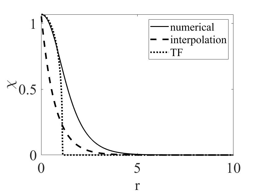
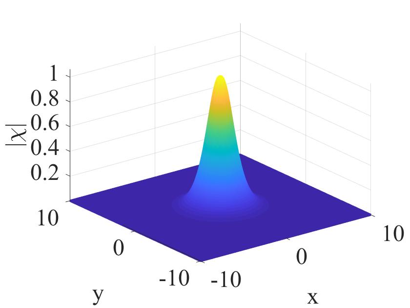
Figure 1: (a) The radial profile of a (stable) numerically found GS and its TF and interpolation counterparts, produced by Eqs. (21), (45), and (32), respectively, with $\sigma=0$, $U_{0}=2$, and $\mu=-1$. The total norm of the numerical, TF, and interpolation solutions are, severally, $N_{\mathrm{num}}=10.34$, $N_{\mathrm{TF}}=9.28$, and $N_{\mathrm{interpol}}=4.86$. (b) The global shape of the numerically generated solution.

Further, Fig. 2 displays the GS, along with the corresponding TF approximation, for sufficiently large $U_{0}=10$. It is seen that, as expected, the TF solution is virtually identical to the numerical one at $r<r_{0}\approx\allowbreak 2.\,\allowbreak 24$, see Eq. (45), while the decaying tail is ignored by TF. In this case, the discrepancy in the total norm is $\left(N-N_{\mathrm{TF}}\right)/N\approx 3.3\%$.

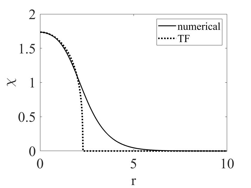
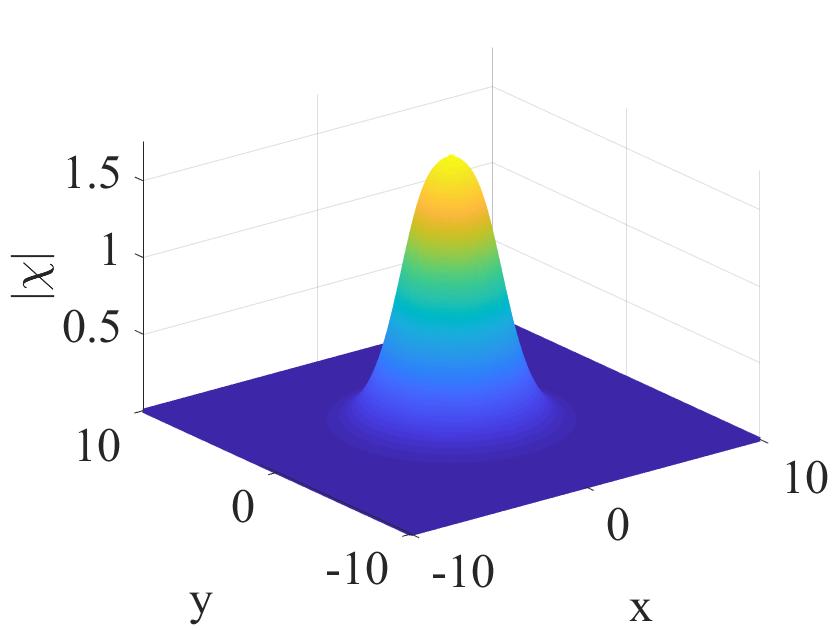
Figure 2: The same as in Fig. 1, but for $U_{0}=10$ and without showing the interpolation given by Eq. (32), which is irrelevant in this case. The norms of the numerical and approximate solutions are $N_{\mathrm{num}}=41.05$, $N_{\mathrm{TF}}=39.68$.

The effect of the MF cubic term of either sign, repulsive ($\sigma=1$) or attractive ($\sigma=-1$) on the shape of the GS is illustrated by Fig. 3. At $r=0$, all the three shapes converge to a common value, $\chi(r=0)\approx 1.20$, exactly as predicted by Eq. (22).

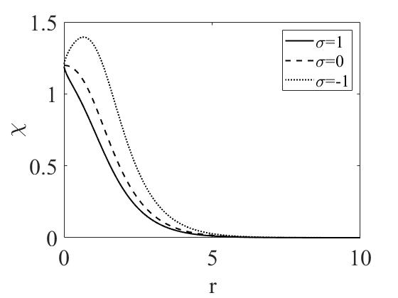
Figure 3: Examples of numerically found stable GS solutions of Eq. (21) for $l=0,U_{0}=3,\mu=-0.8$ , and $\sigma=1$, $0$, and $-1$. The respective norms are $N(\sigma=1)=11.7$, $N(\sigma=0)=15.41$ and $N(\sigma=-1)=24.62$.

The above counterintuitive prediction of the GS solutions existing in the presence of the repulsive potential, with $U_{0}$ belonging to interval (24), is confirmed by numerical results. As an example, Fig. 4 displays stable GSs which were found, in the numerical form, at $U_{0}=-0.4$, taken close to the edge of the interval, $U_{0}=-4/9$, for all the three essential values, $\sigma=0$ and $\pm 1$, of the coefficient in front of the MF cubic repulsive term. The figure shows that the interpolating approximation, generated by Eq. (32), is quite accurate in this case, while the MF cubic term produces a weak effect on the solution. As for the TF approximation (45), it does not apply to $U_{0}<0$.

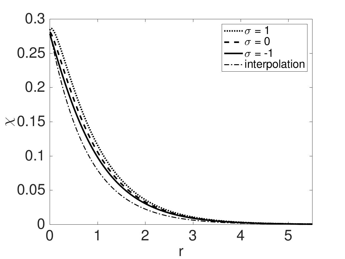
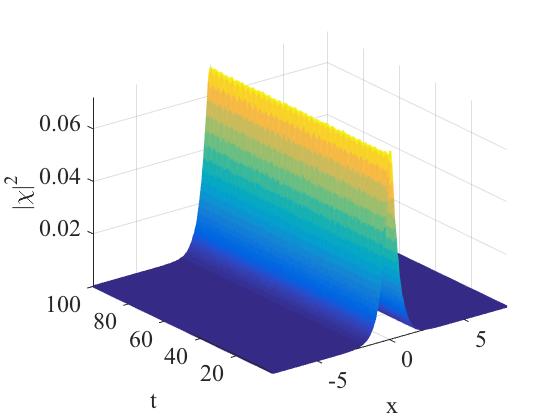
Figure 4: (a) Radial profiles of stable GS modes, produced by the numerical solution of Eq. (21), and by interpolation (32), in the presence of the repulsive potential, with $U_{0}=-0.4$, at $\mu=-0.8$, without and with the MF repulsive or attractive cubic term ($\sigma=0$ and $\sigma=1$ or $-1$, respectively). The corresponding values of the norm are $N\left(\sigma=1\right)=0.41$, $N(\sigma=0)=0.45$, and $N(\sigma=-1)=0.52$, the interpolating approximation giving $N\approx 0.36$, pursuant to Eq. (33). (b) Confirmation of the stability of the GS mode in direct simulations, in the case of $\sigma=1$.

Families of the GS solutions are characterized by the corresponding dependences $N(\mu)$. These results are summarized in Figs. 5(a,b) for the 2D system without and with the MF repulsive or attractive cubic term, $\sigma=0$ and $\sigma=\pm 1$, and for several values of strength $U_{0}$ of the central potential (including both $U_{0}>0$ and $U_{0}<0$). In particular, the MF cubic term produces a more considerable effect with the increase of $U_{0}$, which is naturally explained by the fact that the solution’s amplitude is larger for larger $U_{0}$, as per Eqs. (22), (32), and (45). The $N(\mu)$ curves produced by the TF approximation pursuant to Eq. (46) are compared to their numerical counterparts in panel (a). As mentioned above, the accuracy of the TF approximation essentially improves with the increase of $U_{0}$. On the other hand, interpolating approximation produces poor accuracy at $U_{0}>0$, but for $U_{0}=-0.4$ this approximation is virtually identical to the numerical counterpart.

Panel (c) in Fig. 5 confirms that, in the presence of the attractive cubic term ($\sigma=-1$), the GS exists at $|\mu|>\left(|\mu|\right)_{\mathrm{thr}}$, as predicted by the TF approximation in Eq. (50). Up to the accuracy of the numerical results, the threshold value of $|\mu|$ is indeed $4/27$, in agreement with Eq. (50). This finding is explained by the fact that, as it follows from Eq. (49), the width of the GS diverges in the limit of $|\mu|\rightarrow\left(|\mu|\right)_{\mathrm{thr}}$, hence in this limit the spatial derivatives in Eq. (14) become negligible, and the TF approximation becomes asymptotically exact. Strictly speaking, $N(\mu)$ steeply diverges in the limit of $|\mu|\rightarrow 4/27$, according to Eq. (51), but it is difficult to plot the curves very close to the threshold, as the bound states become extremely broad in this limit.

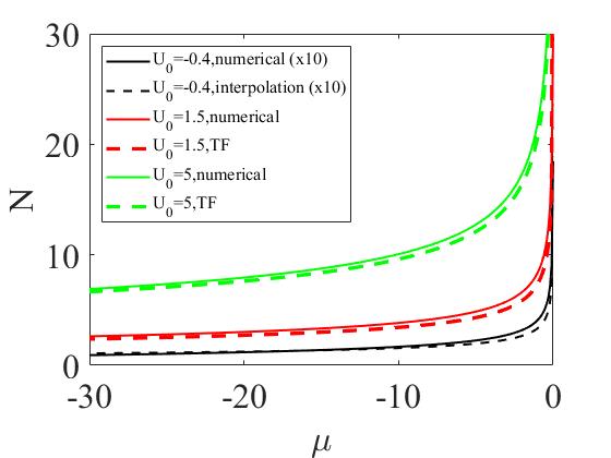
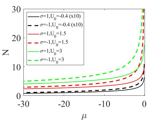
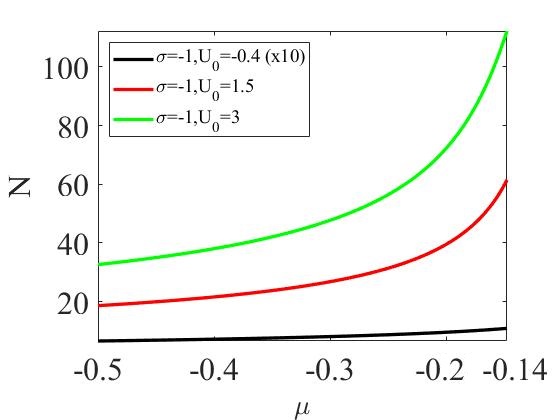
Figure 5: Dependences $N(\mu)$ for stable GS solutions with $U_{0}=-0.4$, and $N(\mu)$ for $U_{0}=$ $1.5$, $3.0$, $5.0$, which correspond, respectively, to the repulsive and attractive central potential. To plot the curve for $U_{0}=-0.4$, values of $N$ are multiplied by $10$, as the actual values of the norm are too small in this case. Panels (a) and (b) correspond to the system which does or does not include the repulsive or attractive cubic term ($\sigma=0$ and $1,-1$, respectively). In (a), the numerical results are compared to the analytical ones, predicted by the TF approximation, as per Eq. (46) [except for the case of $U_{0}=-0.4$, where the TF approximation is irrelevant; however, in this case the analytical prediction given by the interpolating approximation, in the form of Eq. (33), completely overlaps with the numerically generated curve]. In (b), the numerically generated curves are compared for $\sigma=1$ and $-1$. Panel (c) displays a zoom of the plot from (b) at small values of $|\mu|$, with the aim to show the proximity to the threshold value $\left(|\mu|\right)_{\mathrm{thr}}=4/27\approx\allowbreak 0.15$ for $\sigma=-1$, as predicted in the TF approximation by Eq. (50) (see further comments, concerning this point, in the text).

Concerning the stability, both the computation of eigenvalues for small perturbations and direct simulations of perturbed evolution demonstrate complete stability of the fundamental (GS) solutions at all values of $U_{0}$, both positive ones and negative values belonging to interval (24), and at all (negative) values of $\mu$. As an illustration, Fig. 4(b) demonstrates the stability of the GS in the counterintuitive case of the repulsive central potential, with $U_{0}=-0.4$. The stability does not depend either on the presence of the MF cubic term, being equally valid for $\sigma=0$ and $\pm 1$. Note also that the anti-VK stability criterion, $dN/d\mu>0$, holds for all $N(\mu)$ curves in Fig. 5.

III.2 Vortex modes

As mentioned above, the stationary shape of vortex modes, given by Eq. (13) with $l\geq 1$, is actually the same as for the GS with $l=0$, the difference amounting to replacement of $U_{0}$ by $U_{l}~{}$as per Eq. (15). A typical example of the vortex solution with $U_{0}=1.53$ and $l=1$ is displayed in Fig. 6 [as it follows from Eqs. (21) and (15), its amplitude profile is the same as that of the GS with $U_{0}=0.53$]. This value of $U_{0}$ is chosen in the instability region, close to its boundary predicted by Eq. (44), $\left(U_{0}\right)_{\mathrm{crit}}^{(l=1)}\approx\allowbreak 1.56$ [see also Fig. 7(a) below].

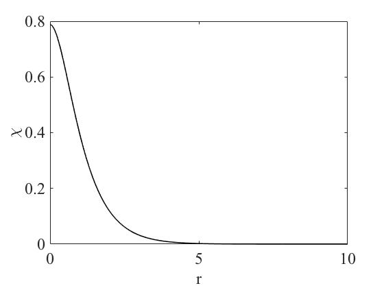
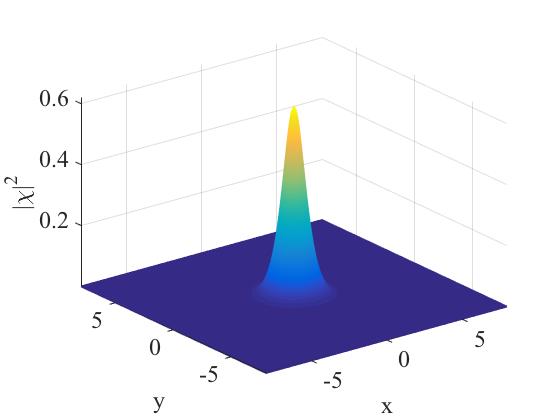
Figure 6: The amplitude structure of an (unstable) vortex mode with $l=1$ in Eq. (13), numerically generated for $\sigma=0$, $U_{0}=1.53$ and $\mu=-1$: (a) the radial profile; (b) the global shape. The total norm of the vortex mode, computed as per Eq. (19), is $N\approx 4.58$.

Differently from the GS, vortex modes are only partially stable, as demonstrated by values of the eigenvalues for small perturbations, produced by the numerical solution of BdG equations (35), and by direct simulations of Eq. (20) alike. We have performed a systematic stability analysis for the vortex modes with $l=1$, in the case of $\sigma=0$ [no MF cubic term in Eq. (9)]. First, it was found that, up to accuracy of the numerically accumulated data, all eigenvalues have zero real parts at $U_{0}>14/9$, and, in exact agreement with Eq. (44), pairs of unstable eigenvalues appear at $U_{0}<14/9$. Also in agreement with the above derivation, the respective eigenmodes of small perturbations correspond to $m=\pm 1$ in Eq. (42), i.e., they are dipole modes, which initiate spontaneous drift of the vortex’ pivot off the central point. An illustration of the resulting instability development is provided by Fig. 7(a), which shows that the drift instability triggers motion of the center of mass (CM) of the vortex mode along the spiral trajectory, the CM’s location being defined as

$$\left\{x_{\mathrm{CM}},y_{\mathrm{CM}}\right\}=\frac{1}{N}\int\int\left\{x_{{}_{\mathrm{CM}}},y_{{}_{\mathrm{CM}}}\right\}\left|\psi\left(x,y\right)\right|^{2}dxdy,$$ (52)

where $N$ is the total norm defined by Eq. (10). Eventually, the pivot will be ousted to periphery, thus effectively converting the unstable vortex mode into a stable GS with zero vorticity. In the case of $U_{0}>14/9$, the simulations demonstrate that a perturbed vortex with $l=1$ is a stable mode which stays at the central position (not shown here in detail).

In the course of the simulations, a large part of the initial norm is consumed by the absorber (emulating losses due to outward emission of small-amplitude matter waves, in the indefinitely extended system). In particular, the evolution of the unstable vortex displayed in Fig. 7(a) leads to its transformation into a residual GS with norm $N=1.88$ ($\approx 41\%$ of the initial value) and chemical potential $\mu\approx-95$, which is completely different from the initial value, $\mu=-1$. Taking into regard that the transformation $l=1\rightarrow l=0$ implies the replacement of $U_{l=1}=U_{0}-l^{2}=0.53$ by $U_{0}=1.53$, see Eq. (15), it is worthy to note that the TF approximation, given by Eqs. (46) with $\mu=-95$, yields a close value of the norm, $N_{\mathrm{TF}}^{(\sigma=0)}(\mu)\approx 1.65$, even if $U_{0}=1.53$ is not a large value.

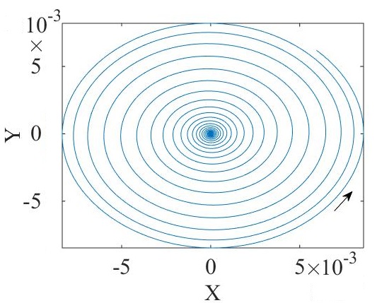
Figure 7: The instability development of the vortex mode with $l=1$ which is shown in Fig. 6. (a) The trajectory of spontaneous motion of the vortex’ CM [see Eq. (52)], initiated by the drift instability, at the initial stage of the evolution. The arrow indicates the direction of the motion along the trajectory. (b) The evolution of the total angular momentum, defined as per Eq. (12), gradually consumed by the edge absorber, illustrates the spontaneous transformation of the unstable vortex into a stable ground state.

The spontaneous transformation of the vortex mode into the GS implies decay of the mode’s angular momentum, $L_{z}$, defined by Eq. (12). In the extended system, the momentum would be lost with emitted matter waves, while in the present setting it is gradually eliminated by the edge absorber. The dependence of $L_{z}$ on time, corresponding to the evolution of the unstable vortex in Fig. 7(a), is shown in Fig. 7(b).

The spiral motion displayed in Fig. 7(a) represents only an initial stage of the evolution [in the notation adopted in Fig. (9), the time interval displayed in this figure is $t=7$]. At large times, when the vortex’s pivot will be lost in the periphery, the CM will eventually return to the central position. In a fully conservative system, the CM would rather orbit the center, cf. Eq. (2), but in the present setting the effective dissipation induced by the absorber makes the return to the center possible.

It is relevant to mention too that, as it follows from Eq. (42), the vortex mode with $l=1$ may become unstable against the perturbation with $m=2$, i.e., against spontaneous splitting in two fragments, at still smaller values of the pull strength, viz., $U_{0}<5/9$. In this work, we did not aim to detect this, apparently weaker, instability, in the simulations. Lastly, for $l=2$ Eq. (43) predicts a much drift-instability region, $U_{0}<77/9$. This instability of the double vortex could be easily detected in the simulations (not shown here in detail).

IV Conclusion

While it was recently demonstrated that the quantum collapse, caused by the potential of attraction to the center $\sim-r^{-2}$, can be suppressed by the cubic repulsive MF (mean-field) nonlinearity in 3D bosonic gases, making it possible to restore the otherwise missing GS (ground state), the cubic self-repulsion is not sufficiently strong to stabilize the gas in the effectively 2D setting. We have demonstrated that the effective quartic repulsion, induced by the LHY (Lee-Huang-Yang) effect, i.e., the correction to the MF theory produced by quantum fluctuations, provides the minimum strength of nonlinearity sufficient for the stabilization of the 2D gas under the action of the same attractive central potential. As a result, the stable GS is created, with a singular but integrable density pattern. The results are obtained in the numerical form, as well as by means of analytical methods, based on the use of asymptotic expansions of the wave functions at $r\rightarrow 0$ and $r\rightarrow\infty$, and TF (Thomas-Fermi) approximation. A counterintuitive finding, an explanation to which is given, is that the stable GS exists even in the case when the central potential is repulsive, provided that its strength does not exceed a critical value. In addition to the completely stable GS, partly stable singular vortex states are constructed too, and their stability boundary is found in an exact form. The pivot of an unstable vortex spontaneously drifts away from the center along a spiral trajectory, the vortex being eventually replaced by a stable GS. An estimate of the underlying physical parameters, which correspond to the realization of the model in the form of the gas of particles carrying permanent electric dipole moments, pulled to the central charge, demonstrates that the radial size of the restored GS may be $R\sim 10$ $\mathrm{\mu}$m, with the expected number of particles $\char 126\relax 10^{5}$.

As an extension of the present analysis, it may be interesting, in particular, to analyze a setting with two mutually symmetric attraction centers, a challenging possibility being prediction of spontaneous breaking of the symmetry in the GS pinned to the pair of the centers.

References

- (1) L. D. Landau and E. M. Lifshitz, Quantum Mechanics: Nonrelativistic Theory (Nauka publishers: Moscow, 1974).
- (2) H. Sakaguchi and B. A. Malomed, Suppression of the quantum-mechanical collapse by repulsive interactions in a quantum gas, Phys. Rev. A 83, 013607 (2011).
- (3) J. Denschlag and J. Schmiedmayer, Scattering a neutral atom from a charged wire, Europhys. Lett. 38, 405 (1997).
- (4) J. Denschlag, G. Umshaus, and J. Schmiedmayer, Probing a singular potential with cold atoms: A neutral atom and a charged wire, Phys. Rev. Lett. 81, 737 (1998).
- (5) K. S. Gupta and S. G. Rajeev, Renormalization in quantum mechanics, Phys. Rev. D 48, 5940(1993).
- (6) H. E. Camblong, L. N. Epele, H. Fanchiotti, and C. A. García Canal, Renormalization of the inverse square potential, Phys. Rev. Lett. 85, 1590 (2000).
- (7) H. E. Camblong, L. N. Epele, H. Fanchiotti, and C. A. García Canal, Dimensional transmutation and dimensional regularization in quantum mechanics: II. rotational invariance, Ann. Phys. (N.Y.) 287, 57 (2001).
- (8) L. Pitaevskii and S. Stringari, Bose-Einstein Condensation (Clarendon Press, Oxford, 2003).
- (9) G. E. Astrakharchik and B. A. Malomed, Quantum versus mean-field collapse in a many-body system, Phys. Rev. A 92, 043632 (2015).
- (10) H. Sakaguchi and B. A. Malomed, Suppression of the quantum collapse in an anisotropic gas of dipolar bosons, Phys. Rev. A 84, 033616 (2011).
- (11) H. Sakaguchi and B. A. Malomed, Suppression of the quantum collapse in binary bosonic gases, Phys. Rev. A 88, 043638 (2013).
- (12) B. A. Malomed, Suppression of quantum-mechanical collapse in bosonic gases with intrinsic repulsion: a brief review, Condensed Matter 3, 15 (2018).
- (13) S. K. Adhikari and L. Salasnich, One-dimensional superfluid Bose-Fermi mixture: Mixing, demixing, and bright solitons, Phys. Rev. A 76, 023612 (2007).
- (14) A. Bulgac, Local-density-functional theory for superfluid fermionic systems: The unitary gas, Phys. Rev. A 76, 050402(R) (2007).
- (15) S. K. Adhikari, Superfluid Fermi-Fermi mixture: Phase diagram, stability, and soliton formation, Phys. Rev. A 76, 053609 (2007).
- (16) S. K. Adhikari, Nonlinear Schrödinger equation for a superfluid Fermi gas in the BCS-BEC crossover, Phys. Rev. A 77, 045602 (2008).
- (17) F. K. Abdullaev, A. Gammal, L. Tomio, and T. Frederico, Stability of trapped Bose-Einstein condensates, Phys. Rev. A 63, 043604 (2001).
- (18) F. K. Abdullaev and M. Salerno, Gap-Townes solitons and localized excitations in low-dimensional Bose-Einstein condensates in optical lattices, Phys. Rev. A 72, 033617 (2005).
- (19) E. A. Burt, R. W. Ghrist, C. J. Myatt, M. J. Holland, E. A. Cornell, and C. E. Wieman, Coherence, correlations, and collisions: What one learns about Bose-Einstein condensates from their decay, Phys. Rev. Lett. 79, 337 (1997).
- (20) D. M. Stamper-Kurn, M. R. Andrews, A. P. Chikkatur, S. Inouye, H. J. Miesner, J. Stenger, and W. Ketterle, Optical confinement of a Bose-Einstein condensate, Phys. Rev. Lett. 80, 2027 (1998).
- (21) J. L. Roberts, N. R. Claussen, S. L. Cornish, and C. E. Wieman, Magnetic field dependence of ultracold inelastic collisions near a Feshbach resonance, Phys. Rev. Lett. 85, 728 (2000).
- (22) D. S. Petrov, Quantum mechanical stabilization of a collapsing Bose-Bose mixture, Phys. Rev. Lett. 115, 155302 (2015).
- (23) D. S. Petrov, and G. E. Astrakharchik, Ultradilute low-dimensional liquids, Phys. Rev. Lett. 117, 100401 (2016).
- (24) P. Żin, M. Pylak, T. Wasak, M. Gajda, and Z. Idziaszek, Quantum Bose-Bose droplets at a dimensional crossover, Phys. Rev. A 98, 051603(R) (2018).
- (25) T. Ilg, J. Kumlin, L. Santos, and D. S. Petrov, and, H. P. Büchler, Dimensional crossover for the beyond-mean-field correction in Bose gases, Phys. Rev. A 98, 051604 (2018).
- (26) T. D. Lee, K. Huang, and C. N. Yang, Eigenvalues and eigenfunctions of a Bose system of hard spheres and its low-temperature properties, Phys. Rev. 106, 1135-1145 (1957).
- (27) S. Roy, M. Landini, A. Trenkwalder, G. Semeghini, G. Spagnolli, A. Simoni, M. Fattori, M. Inguscio, and G. Modugno, Test of the universality of the three-body Efimov parameter at narrow Feshbach resonances, Phys. Rev. Lett. 111, 053202 (2013).
- (28) C. Cabrera, L. Tanzi, J. Sanz, B. Naylor, P. Thomas, P. Cheiney, and L. Tarruell, Quantum liquid droplets in a mixture of Bose-Einstein condensates, Science 359, 301-304 (2018).
- (29) P. Cheiney, C. R. Cabrera, J. Sanz, B. Naylor, L. Tanzi, and L. Tarruell, Bright soliton to quantum droplet transition in a mixture of Bose-Einstein condensates, Phys. Rev. Lett. 120, 135301 (2018).
- (30) G. Semeghini, G. Ferioli, L. Masi, C. Mazzinghi, L. Wolswijk, F. Minardi, M. Modugno, G. Modugno, M. Inguscio, and M. Fattori, Self-bound quantum droplets of atomic mixtures in free space, Phys. Rev. Lett. 120, 235301 (2018).
- (31) G. Ferioli, G. Semeghini, L. Masi, G. Giusti, G. Modugno, M. Inguscio, A. Gallemi, A. Recati, and M. Fattori, Collisions of self-bound quantum droplets, Phys. Rev. Lett. 122, 090401 (2019).
- (32) C. D’Errico, A. Burchianti, M. Prevedelli, L. Salasnich, F. Ancilotto, M. Modugno, F. Minardi, and C. Fort, Observation of quantum droplets in a heteronuclear bosonic mixture, Phys. Rev. Research 1, 033155 (2019).
- (33) Y. Li, Z. Luo, Y. Lio, Z. Chen, C. Huang,S. Fu, H. Tan, and B. A. Malomed, Two-dimensional solitons and quantum droplets supported by competing self- and cross-interactions in spin-orbit-coupled condensates, New J. Phys. 19, 113043 (2017).
- (34) Y. Li, Z. Chen, Z. Luo, C. Huang, H. Tan,W. Pang, and B. A. Malomed, Two-dimensional vortex quantum droplets, Phys. Rev. A 98, 063602 (2018).
- (35) M. Nilsson Tengstrand, P. Stürmer, E. Ö. Karabulut, and S. M. Reimann, Rotating binary Bose-Einstein condensates and vortex clusters in quantum droplets, Phys. Rev. Lett. 123, 160405 (2019).
- (36) Y. V. Kartashov, B. A. Malomed, L. Tarruell, and L. Torner, Three-dimensional droplets of swirling superfluids, Phys. Rev. 98, 013612 (2018).
- (37) H. Kadau, M. Schmitt, M. Wentzel, C. Wink, T. Maier, I. Ferrier-Barbut, and T. Pfau, Observing the Rosenzweig instability of a quantum ferrofluid, Nature 530, 194-197 (2016).
- (38) M. Schmitt, M. Wenzel, 491 F. Böttcher, I. Ferrier-Barbut and T. Pfau, Self-bound droplets of a dilute magnetic quantum liquid, Nature 539, 259-262 (2016).
- (39) I. Ferrier-Barbut, H. Kadau, M. Schmitt, M. Wenzel, and T. Pfau, Observation of quantum droplets in a strongly dipolar Bose gas, Phys. Rev. Lett. 116, 215301 (2016).
- (40) F. Wächtler and L. Santos, Ground-state properties and elementary excitations of quantum droplets in dipolar Bose-Einstein condensates, Phys. Rev. A 94, 043618 (2016).
- (41) D. Baillie and P. B. Blakie, Droplet crystal ground states of a dipolar Bose gas, Phys. Rev. Lett. 121, 195301 (2018).
- (42) A. Cidrim, F. E. A. dos Santos, E. A. L. Henn, and T. Macrí, Vortices in self-bound dipolar droplets, Phys. Rev. A 98, 023618 (2018).
- (43) N. B. Jørgensen, G. M. Bruun, and J. J. Arlt, Dilute fluid governed by quantum fluctuations, Phys. Rev. Lett. 121, 173403 (2018).
- (44) L. Salasnich, A. Parola, and L. Reatto, Effective wave equations for the dynamics of cigar-shaped and disk-shaped Bose condensates, Phys. Rev. A 65, 043614 (2002).
- (45) A. Muñoz Mateo and V. Delgado, Effective mean-field equations for cigar-shaped and disk-shaped Bose-Einstein condensates, Phys. Rev. A 77, 013617 (2008).
- (46) H. Sakaguchi and B. A. Malomed, Solitons in combined linear and nonlinear lattice potentials, Phys. Rev. A 81, 013624 (2010).
- (47) N. G. Vakhitov and A. A. Kolokolov, Stationary solutions of the wave equation in a medium with nonlinearity saturation, Radiophys. Quantum Electron. 16, 783-789 (1973).
- (48) L. Bergé, Wave collapse in physics: principles and applications to light and plasma waves, Phys. Rep. 303, 259-370 (1998).
- (49) L. Veron, Singular solutions of some nonlinear elliptic equations, Nonlinear Analysis, Theory, Methods & Applications 5, 225-242 (1981).
- (50) H. Sakaguchi and B. A. Malomed, Singular solitons, Phys. Rev. E 101, 012211 (2020).
- (51) E. Shamriz, Z. Chen, B. A. Malomed, and H. Sakaguchi, Singular mean-field states: a brief review of recent results, Condensed Matter 5, 20 (2010).
- (52) J. Yang, Nonlinear Waves in Integrable and Nonintegrable Systems (SIAM, Philadelphia, 2010).
- (53) B. A. Malomed, D. Mihalache, F. Wise, and L. Torner, Spatiotemporal optical solitons, J. Optics B: Quant. Semicl. Opt. 7, R53-R72 (2005).