Asymptotics of Lower Dimensional Zero-Density Regions

Abstract

Topological data analysis (TDA) allows us to explore the topological features of a dataset. Among topological features, lower dimensional ones have recently drawn the attention of practitioners in mathematics and statistics due to their potential to aid the discovery of low dimensional structure in a data set. However, lower dimensional features are usually challenging to detect based on finite samples and using TDA methods that ignore the probabilistic mechanism that generates the data. In this paper, lower dimensional topological features occurring as zero-density regions of density functions are introduced and thoroughly investigated. Specifically, we consider sequences of coverings for the support of a density function in which the coverings are comprised of balls with shrinking radii. We show that, when these coverings satisfy certain sufficient conditions as the sample size goes to infinity, we can detect lower dimensional, zero-density regions with increasingly higher probability while guarding against false detection. We supplement the theoretical developments with the discussion of simulated experiments that elucidate the behavior of the methodology for different choices of the tuning parameters that govern the construction of the covering sequences and characterize the asymptotic results.

1 Introduction

We consider the problem of identifying certain lower-dimensional, geometric features of (the support of) a density that generates a stream of observed data. What makes this identification at once interesting and challenging is that the features we are concerned with cannot be detected using any finite amount of data. Typical topological data analysis (TDA) techniques would be unsuitable in this context because they rely on the relative arrangement of points in finite data sets to understand the structure of the (sub)-space where the data occur (see for example [5, 6] and [11] for introductory treatments). We can make progress in the detection process because we rely on knowledge of relevant distributional properties of the data generating mechanism that we acquire as more and more data accrue. This is in contrast to a standard use of TDA methods that would not explicitly account for these distributional properties. We study the asymptotics of the data generating mechanism directly and show that they can be linked to certain topological characteristics.

In this paper, we first discuss situations where independent and identically distributed (i.i.d.) data points are drawn from a distribution having a continuous density function $f$ (with respect to Lebesgue measure on $\mathbb{R}^{d}$) on its support $supp(f)=M\subset\mathbb{R}^{d}$. Our results are first formally stated for $supp(f)=M=[0,1]^{d},$ $d\in\mathbb{N}$, and then extended to more general situations. We work with a well-behaved version of the density $f$ for which the notion of a zero-density region $S_{0}\subset supp(f)\subset M$ (to be formally defined later) is meaningful. Such a zero-density region $S_{0}$ is difficult to identify with traditional constructions of simplices or density estimators.

Example 1.1.

Let $S_{0}=\{\frac{1}{2}\}\times[0.25,0.75]$ and define $d(\boldsymbol{x},S_{0})=\inf_{\boldsymbol{y}\in S_{0}}d(\boldsymbol{x},\boldsymbol{y})$, where $d$ denotes the $L^{2}$ metric. Consider the density $f(\boldsymbol{x})\propto d(\boldsymbol{x},S_{0})^{4}\circ\boldsymbol{1}_{[0,1]^{2}}$ shown in Figure 1, for which $S_{0}$ is a zero density region of lower dimension. $S_{0}$ does not contain any probability mass and, being a segment, is a “lower dimensional object” (a concept to be made more precise later).

The volume of $S_{0}$ as a subset of the support of the density, $[0,1]^{2}$, is zero and the density assigns positive probability to every neighborhood of every point in $S_{0}$. Sampled points “on either side” of $S_{0}$ can be arbitrarily close to one another. Hence, it might seem to be impossible to identify the topological structure of $S_{0}$ with accuracy. However, consideration of an asymptotic argument that relies on the rate at which points accumulate in the vicinity of $S_{0}$ as the sample size grows allows us to identify the structure of $S_{0}$. We note that the situation would be different if the density were zero on a region of positive volume, such as a disk, and nonzero elsewhere. The disk could then be identified with a large enough sample as a “hole” not containing any points.

Our upcoming results consider samples of increasing size. The main result allows us to detect the lower dimensional object $S_{0}$ with probability one as the sample size $n$ goes to infinity, while at the same time helping us avoid detection of false holes.

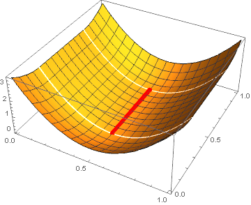
Figure 1: A lower dimensional region $S_{0}=\{\frac{1}{2}\}\times[0.25,0.75]$ (red segment) for the density function $f(\boldsymbol{x})\propto d(\boldsymbol{x},S_{0})^{4}\circ\boldsymbol{1}_{[0,1]^{2}}(\boldsymbol{x})$, where $d(\boldsymbol{x},S_{0})=\inf_{\boldsymbol{y}\in S_{0}}d(\boldsymbol{x},\boldsymbol{y})$ and $d$ denotes Euclidean distance. The density $f$ evaluates to 0 over $S_{0}$, but nowhere else over $[0,1]^{2}$.

Our approach to detecting zero-density regions is to conduct an analysis as we vary the radius of a collection of covering balls of $supp(f)$. By choosing the shared radius of the covering balls appropriately relative to increasing sample size $n$, we wish that $S_{0}$ be covered only by balls having no observations inside. For each point in the non-zero density region we wish for the point to eventually be covered by a ball with at least one observation inside. If our wishes come true, then we can simply collect the empty covering balls and recover an approximation to the region $S_{0}$. In Theorem 3.11 we present a set of sufficient conditions for our detection method to work asymptotically.

This notion of varying the radius of the covering balls can be related to the construction of complexes in TDA. For the Čech complex, balls are centered at the observed points. Balls of a fixed radius $r$ lead to a Čech complex $C(\mathcal{X},r)$. Varying the radius $r$, the Čech filtration, a collection of Čech complexes, is produced. For a small radius $r$, the balls will not overlap and no holes will be discovered. For a large radius $r$, lower dimensional zero-density regions will be covered and these holes will not be found.

The rest of the paper is organized as follows. We first illustrate our observations above with a simple example in Section 2. Then, in Section 3, we discuss our approach for the construction of coverings of a compact support along with a set of sufficient conditions that ensure asymptotic consistency of the procedure for the detection of zero-density regions. Generalizations of the results to the case of a non-compact support are provided in Section 4. We present some experimental results and connections to other areas in Section 5 and end with a brief discussion of our findings in Section 6.

2 An Illustrative Example

The central problem we investigate in this paper is the detection of a lower dimensional zero-density region. Before formally addressing the problem, we present an illustrative example to show how dimensionality plays an important role.

We consider three different densities on the interval $M=[-1,1]$, $\dim M=1$, and the problem of detecting interesting topological features by partitioning $M$ into the union of disjoint, equally sized bins. The feature (or lack thereof) for two of the densities is easily found. The density $g(x)=\frac{2}{3}\left(\boldsymbol{1}_{[-1,-1/4]}(x)+\boldsymbol{1}_{[1/4,1]}(x)\right)$ has a genuine hole, $(-1/4,1/4)$, consisting of an interval of dimension one. This hole is apparent, as there will never be any observations in it, nor in bins contained in it. As the sample size $n$ goes to infinity, one need only consider bins whose widths decrease at a rate no faster than $n^{-1+\varepsilon}$, $\varepsilon>0$, to ensure that the bins away from the hole are eventually filled. When $S_{0}=\emptyset$, as is the case for the density $h(x)=\frac{3}{8}\boldsymbol{1}_{[-1,1]}(x)\cdot\left(x^{2}+1\right)$, and the width of the bins decreases at a rate no faster than $n^{-1+\varepsilon}$, all of the bins will eventually be filled and it will be evident that there is no topological feature.

The interesting case has $S_{0}\neq\emptyset$ and $\dim S_{0}<\dim M=1$, as is the case for $f(x)=\frac{3}{2}x^{2}\boldsymbol{1}_{[-1,1]}(x)$. Here, $S_{0}=\{0\}$, and the question is whether we can detect this topological feature of dimension zero with positive probability. The hole is difficult to detect because samples will accumulate in every neighborhood of $S_{0}=\{0\}$. If the bins shrink too slowly, the sequence of bins that contain $\{0\}$ will be filled as the sample size $n$ goes to infinity.

In Figure 2, the binary heatmaps show the denseness of the non-empty bins. The first column represents histograms and heatmaps for the density $f$ with a zero-dimensional hole $\{0\}$. The second column represents histograms and heatmaps for the density $g$ with a one-dimensional hole $(-1/4,1/4)$. The third column represents histograms and heatmaps for the density $h$ with no holes. The top row is for a small sample size; the bottom row for a larger sample size.

$f(x)=\frac{3}{2}x^{2}\boldsymbol{1}_{[-1,1]}(x)$ $g(x)=\frac{2}{3}\left(\boldsymbol{1}_{[-1,-\frac{1}{4}]}(x)+\boldsymbol{1}_{[\frac{1}{4},1]}(x)\right)$ $h(x)=\frac{3}{8}\boldsymbol{1}_{[-1,1]}(x)\cdot\left(x^{2}+1\right)$

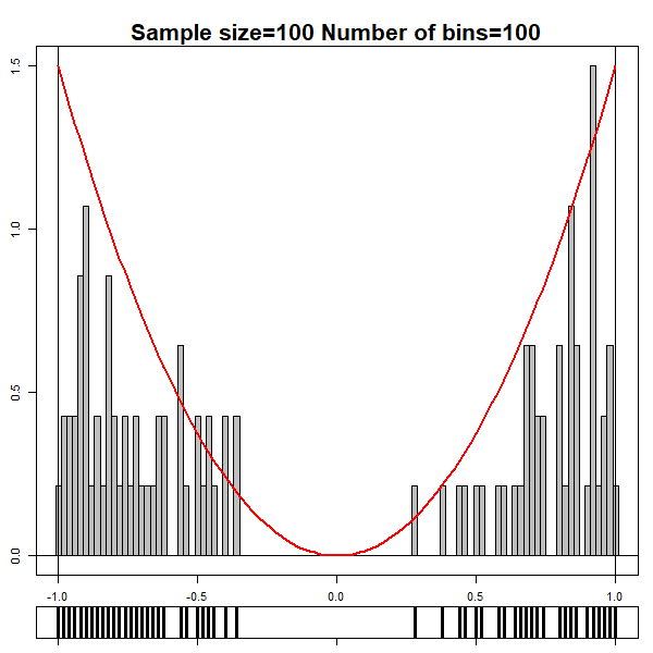
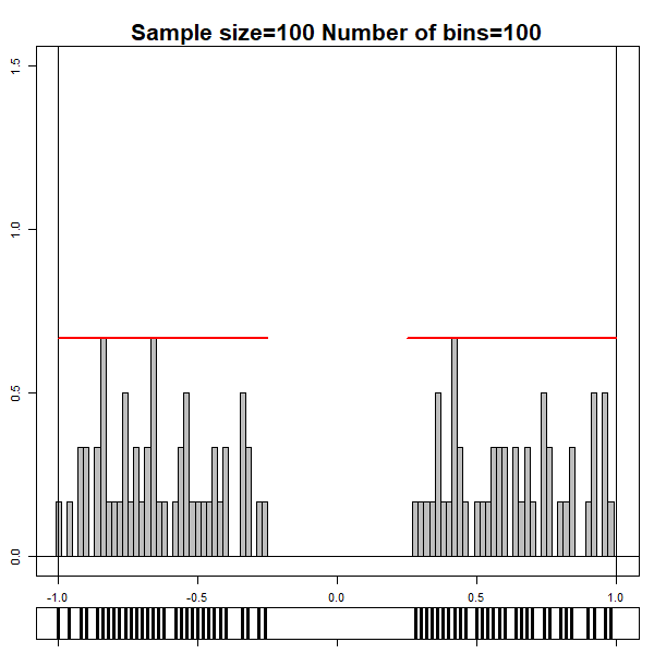
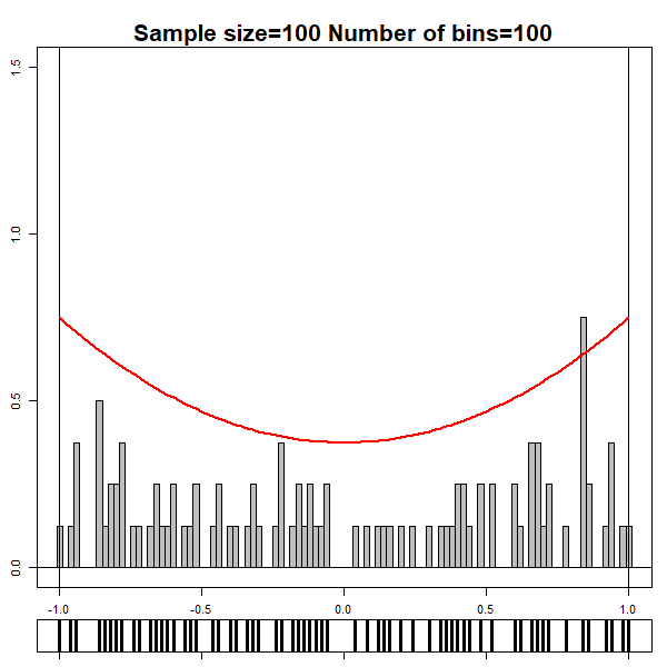
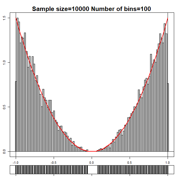
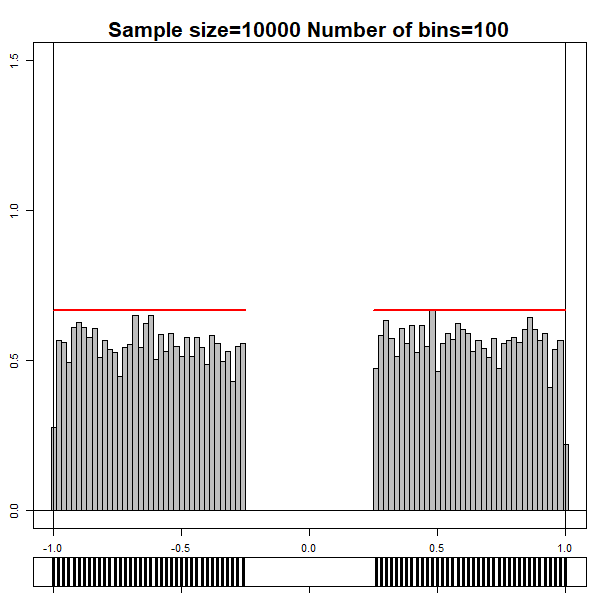
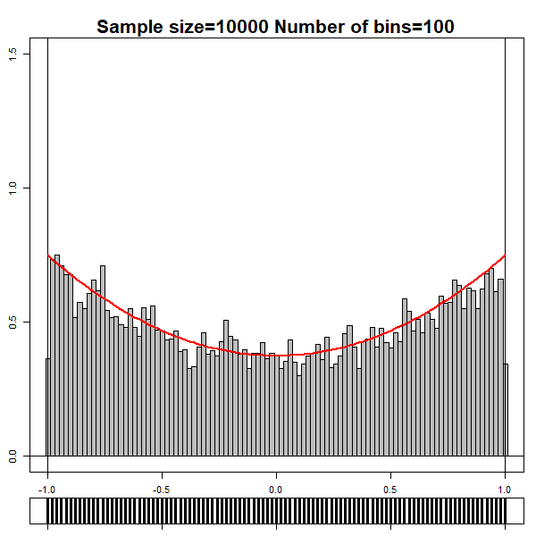
Figure 2: Binned histogram and binary heatmaps based on random samples of size $n=100$ and $n=10,000$ from three distributions with densities $f$, $g$, and $h$. All graphical summaries are constructed using 100 equal-width bins over the interval $[-1,1]\subset\mathbb{R}$.

The figure shows the ease with which binning identifies densities bounded away from $0$. See the filled bins under the red lines in the second and third columns. The figure also shows the ease with which a hole of full dimension is found. See the empty bins in the center of the plots in column two. The difficult case appears in the first column. Here, we see a lower-dimensional hole in the density. The figure suggests that, as the sample size $n$ goes to infinity, we should be able to detect this hole by using binary heatmaps with an appropriate scaling scheme. This is perhaps surprising, because the density $f$ in the first column has full support. Formally, our Theorem 3.11 shows that, if we shrink the common width of the bins (which corresponds to the radius of the covering balls in higher dimensions) at an appropriate rate as a function of sample size $n$, the lower dimensional holes will be characterized in terms of empty bins with probability tending to one. This result can be extended to more general situations.

The objective of this article is to show that, without appropriate scaling, authentic topological holes of strictly lower dimension cannot be detected, while, with appropriate scaling, they can. The sufficient conditions that we will impose on the scaling schemes to attain these results depend on the dimension of the zero-density region $S_{0}$ and also on the local smoothness of the density that generates the data.

3 Main Result for Compact Support

Consider a random vector $X$ having density $f$ with respect to Lebesgue measure on $\mathbb{R}^{d}$. For any Borel set $A\in\mathbb{R}^{d}$, let $P(X\in A)=\int_{A}f(x)\,dx$.

Definition 3.1.

(Support) The support of $X$ is defined to be

$$supp(X) \coloneqq\cap_{\{R_{X}\text{ closed in }\mathbb{R}^{d}\mid P(X\in R_{X})=1\}}R_{X}.$$ (1)

With an abuse of notation, we write $supp(f)$ to represent the support of $X$.

In most applications where TDA is employed, a compact support $M$ can be reasonably assumed. For technical convenience, we will also assume the existence of a continuous version of the density $f$ on its support $M$. The latter is a mild condition satisfied for most theoretical questions and applied scenarios. In the following discussion, as will be stated in Assumption 1 on page 3.8, we consider the case of $M=[0,1]^{d}\subset\mathbb{R}^{d},d>0$. With this particular $M$ in mind, we turn to a special region called the zero-density region assumed to lie in its interior.

Definition 3.2.

(Zero-density region) For the continuous version of a density $f$ on $M$, we call the inverse image of $\{0\}$, i.e. $f^{-1}(\{0\})$, the zero-density region of $f$ and denote it by $S_{0}$.

In a first result (Theorem 3.11), we suppose that $S_{0}$ consists of a single, connected component (as in Assumption 2) for simplicity. We then extend the initial result to the case where $S_{0}$ consists of a finite number of connected components in Corollary 3.12.

The local behavior of the density $f$ around the zero-density region $S_{0}\subset M$ is a crucial aspect of our investigation. The following concepts will help us to describe the behavior of $f$ near $S_{0}$. We consider the $L^{2}$ metric and the associated norm, $\|\cdot\|$, in the following discussion, but remark that our methods can be generalized to other metrics and norms.

A ball of radius $r$ centered at $\boldsymbol{x}$ in $\mathbb{R}^{d}$ is the open set

$$B_{r}(\boldsymbol{x})\coloneqq\left\{\left.\boldsymbol{y}\in\mathbb{R}^{d}\,\right|\|\boldsymbol{x}-\boldsymbol{y}\|<r\right\}$$ .

An $\epsilon$-neighborhood ($\epsilon>0$) of $S_{0}$ is the open set

$$B_{\epsilon}(S_{0})\coloneqq\left\{\boldsymbol{x}\in\mathbb{R}^{d}\left|\,\inf_{\boldsymbol{y}\in S_{0}}\|\boldsymbol{x}-\boldsymbol{y}\|<\epsilon\right.\right\}$$ .

(Note that the definition of an an $\epsilon$-neighborhood makes sense for an arbitrary set, not just a zero-density region. In particular, the $\epsilon$-neighborhood of a point $\boldsymbol{y}$, $B_{\epsilon}(\boldsymbol{y})$, is just the open ball of radius $\epsilon$ centered at $\boldsymbol{y}$.)

Definition 3.3.

(Upper and lower $\epsilon$-order of smoothness) We consider densities $f$ for which the following quantities, called the upper and lower $\epsilon$-order of smoothness, respectively, exist and are well-defined for every $0<\epsilon<1$:

$$\overline{K_{f}}(\epsilon)\coloneqq\inf\left\{\alpha>0\left|0<\inf_{\boldsymbol{x}\in B_{\epsilon}(S_{0})\backslash S_{0}}\frac{f(\boldsymbol{x})}{d(\boldsymbol{x},S_{0})^{\alpha}}\right.\right\},$$

and

$$\underline{K_{f}}(\epsilon)\coloneqq\sup\left\{\alpha>0\left|\infty>\sup_{\boldsymbol{x}\in B_{\epsilon}(S_{0})\backslash S_{0}}\frac{f(\boldsymbol{x})}{d(\boldsymbol{x},S_{0})^{\alpha}}\right.\right\}.$$

Because our result concerns the limiting case as $\epsilon$ goes to zero, we give the following definition.

Definition 3.4.

(Upper and lower order of smoothness) The upper and lower order of smoothness of the density $f$ w.r.t. $S_{0}$, are

$$\overline{K_{f}} =\lim_{\epsilon\rightarrow 0^{+}}\overline{K_{f}}(\epsilon)\,\,\,\text{and}\,\,\,\underline{K_{f}}=\lim_{\epsilon\rightarrow 0^{+}}\underline{K_{f}}(\epsilon),$$

respectively, provided they exist. And if they exist, $\overline{K_{f}}\geq\underline{K_{f}}$ by this definition.

It can be shown that $\overline{K_{f}}$ and $\underline{K_{f}}$ will exist if $\overline{K_{f}}(\epsilon)$ and $\underline{K_{f}}(\epsilon)$ exist for some $\epsilon$ and that there are densities for which $\overline{K_{f}}(\epsilon)$ and $\underline{K_{f}}(\epsilon)$ are undefined for all $\epsilon$. The limits $\overline{K_{f}}$ and $\underline{K_{f}}>0$, if they exist, need not coincide. If they do exist and coincide, we will use the notation $K_{f}=\overline{K_{f}}=\underline{K_{f}}$. Similar but more specific variants of this concept of order of smoothness are studied both in TDA [14] as growth dimensions and in the density estimation literature as local smoothness [22]. The generality of this kind of description makes our assumptions A.1-A.6 for the main theorem (especially A.3-A.4) relevant to research from both communities.

The following example, depicted in Figure 3, shows that the upper and lower orders of smoothness $\overline{K_{f}}$ and $\underline{K_{f}}$ need not coincide.

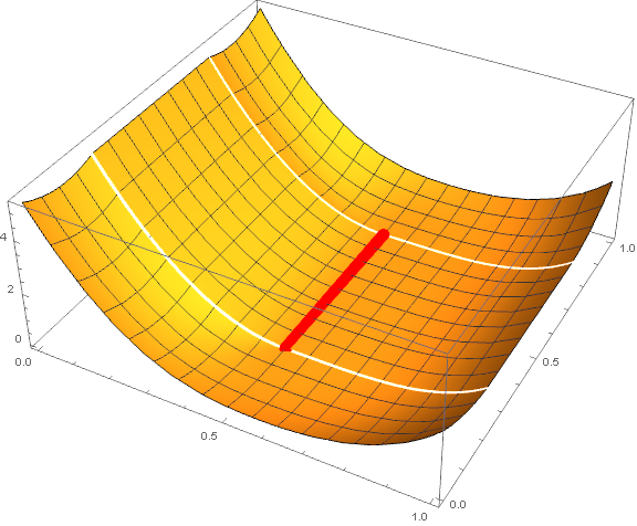
Figure 3: Lower dimensional region $S_{0}=\{\frac{1}{2}\}\times[0.25,0.75]$ of a density function $f(\boldsymbol{x})$ with $\overline{K_{f}}\neq\underline{K_{f}}$. The density $f$ evaluates to 0 over $S_{0}$ but nowhere else over $[0,1]^{2}$.

Example 3.5.

For $\boldsymbol{x}=(x,y)\in\mathbb{R}^{2}$, define $h(\boldsymbol{x})$ as

$$h(\boldsymbol{x})=\begin{cases}d(\boldsymbol{x},S_{0})^{4},&\boldsymbol{x}\in[0.5,1]\times[0.25,0.75],\\ d(\boldsymbol{x},S_{0})^{2},&\boldsymbol{x}\in[0,0.5)\times[0.25,0.75],\\ d(\boldsymbol{x},S_{0})^{4-\frac{2}{\pi}\theta_{1}},&\boldsymbol{x}\in[0,1]\times(0.75,1],\\ d(\boldsymbol{x},S_{0})^{4+\frac{2}{\pi}\theta_{2}},&\boldsymbol{x}\in[0,1]\times[0,0.25),\end{cases}$$

where $d$ is the $L^{2}$ metric, $\theta_{1}=\arctan\{(y-0.75)/(x-0.5)\}$, and $\theta_{2}=\arctan\{(y-0.25)/(x-0.5)\}$. Consider the density function $f$ satisfying the relationship $f(\boldsymbol{x})\propto g(\boldsymbol{x})\times\boldsymbol{1}_{[0,1]^{2}}(\boldsymbol{x})$. For $\boldsymbol{x}\in M$ with $d(\boldsymbol{x},S_{0})=\delta$, $\delta>0$, $\sup_{\boldsymbol{x}}f(\boldsymbol{x})=\delta^{2}$ and $\inf_{\boldsymbol{x}}f(\boldsymbol{x})=\delta^{4}$. Thus $\overline{K_{f}}(\epsilon)=4$ and $\underline{K_{f}}(\epsilon)=2$.

3.1 Covering balls and dimension of $S_{0}$

We cover the support $M$ of the density $f$ with a collection of balls of equal radius and, letting the radius shrink to zero at an appropriate rate, we attempt to detect the zero-density region $S_{0}$ with a certain limiting probability guarantee. In what follows we will make use of the following piece of notation.
Notation. (Covering) Let $E$ be a given subset of $\mathbb{R}^{d}$. We denote by $\mathcal{B}_{r}^{d}(E)$ a collection of $d$-dimensional balls of radius $r$ whose union contains $E$. Note that a covering $\mathcal{B}_{r}^{d}(E)$ may also depend on the sample size $n$ through the radius $r=r(n)$ in subsequent developments. We also use $|\mathcal{B}_{r}^{d}(E)|$ to denote the cardinality of $\mathcal{B}_{r}^{d}(E)$ and write $\mathcal{B}_{r}^{d}(E)=\mathcal{B}$ when the meaning is unambiguous.

We distinguish between three types of covering balls based on how far they are from the zero-density region $S_{0}$.

Definition 3.6.

(Types of covering balls) Consider a density $f$ with respect to Lebesgue measure on $\mathbb{R}^{d}$ that is continuous on $M$ and zero on $\mathbb{R}^{d}\backslash M$. Let $S_{0}$ be a zero-density region for $f$. Denote by $\mathcal{B}$ a covering of $M$ with balls of radius $r$ and let $B_{r}(\boldsymbol{x})\in\mathcal{B}$. We classify $B_{r}(\boldsymbol{x})$ into one of these three types:

1. an $\epsilon$-outside ball: a ball $B_{r}(\boldsymbol{x})$ such that $\boldsymbol{x}\notin B_{\epsilon}(S_{0})$;

2. an $\epsilon$-neighboring ball: a ball $B_{r}(\boldsymbol{x})$ such that $\boldsymbol{x}\in B_{\epsilon}(S_{0})$ and $B_{r}(\boldsymbol{x})\cap S_{0}=\emptyset$;

3. an $\epsilon$-inside ball: a ball $B_{r}(\boldsymbol{x})$ such that $\boldsymbol{x}\in B_{\epsilon}(S_{0})$ and $B_{r}(\boldsymbol{x})\cap S_{0}\neq\emptyset$.

The main result will rely on the condition $r\leq\epsilon/2$ to ensure that every $\epsilon$-inside ball is contained in $B_{\epsilon}(S_{0})$. The various types of covering balls are illustrated in Figure 4.

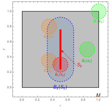
Figure 4: Illustration of the types of balls with the density in Figure 1. The blue region is an epsilon neighborhood surrounding the zero-density region $S_{0}$. The red ball is an $\epsilon$-inside ball, the orange balls are $\epsilon$-neighboring balls and the green balls are $\epsilon$-outside balls.

Definition 3.7.

(Big O notation [4]) Given two positive real sequences $f(n)$ and $g(n)$, we write $f\sim O(g)$ and say that $f$ is big $O$ of $g$ if there exist constants $L_{1}$ and $L_{2}\in(0,\infty)$ and an $n_{0}\in\mathbb{N}$, such that

$${\displaystyle L_{1}\cdot g(n)\leq f(n)\leq L_{2}\cdot g(n)} ,\,\text{for all}\,\,n>n_{0}.$$

This condition means that the asymptotic behaviors of $f$ and $g$ are comparable.

Next, we introduce the notion of Minkowski dimension which we will later use to characterize the dimension of $S_{0}$.

Definition 3.8.

(Minkowski dimension, or box-counting dimension. Definition 3.1 in 12) The upper and lower Minkowski dimensions of a bounded subset $E\subset M$ of $\mathbb{R}^{d}$, are defined respectively as

$$\overline{\dim}_{M}(E) \coloneqq\lim\sup_{\Delta\rightarrow 0}\frac{\log\mathcal{N}_{\Delta}(E)}{-\log\Delta},$$

$$\underline{\dim}_{M}(E) \coloneqq\lim\inf_{\Delta\rightarrow 0}\frac{\log\mathcal{N}_{\Delta}(E)}{-\log\Delta},$$

where $\mathcal{N}_{\Delta}(E)$ is the $\Delta$-covering number of $E\subset\mathbb{R}^{d}$

$$\mathcal{N}_{\Delta}(E) \coloneqq\min\left\{k\in\mathbb{N}\mid E\subset\cup_{i=1}^{k}B_{\Delta}(x_{i})\text{ for some }x_{i}\in\mathbb{R}^{d}\right\},$$

i.e., the smallest number of balls of radius $\Delta>0$ needed to cover $E$. We call this covering of minimal cardinality a minimal $\Delta$-covering for $E$. When $\overline{\dim}_{M}(E)=\underline{\dim}_{M}(E)=d_{M}$, we define the Minkowski dimension (or box-counting dimension) $\dim_{M}(E)$ of $E$ to be $d_{M}$.

By Proposition 3.4 in [12], in the case of $M=[0,1]^{d}$, we always have $\dim_{M}(M)=d$, matching the usual definition of dimension.

We now state the formal assumptions A.1-A.6 which we will use to prove our main results. These assumptions can be put into three groups, as explained after their statements.

1. Global assumptions on $f$, $M$, and $S_{0}$

   A.1. (Compact support) The support of $f$ is $supp(f)=M=[0,1]^{d}$, $d>0$ and we consider the version of the density $f$ that is zero on $\mathbb{R}^{d}\backslash M$ and continuous on $M$.

   A.2. (Single component) The zero-density region $S_{0}$ is contained in the interior of $M$ and has one connected component.

2. Local assumptions on $f$ and $S_{0}$

   A.3. (Order of smoothness) There exists an $\epsilon_{0}>0$ such that both quantities $\overline{K_{f}}(\epsilon_{0})>0$ and $\underline{K_{f}}(\epsilon_{0})>0$ exist. As remarked on page 3.4, the existence of $\epsilon_{0}>0$ implies that the limiting values $\overline{K_{f}}>0$ and $\underline{K_{f}}>0$ also exist.

   A.4. Let $\epsilon_{0}>0$ be as described in A.3. There exist two positive constants $L_{f}$ and $U_{f}$ such that, for all $\epsilon$ with $0<\epsilon<\min(1,\epsilon_{0})$, $L_{f}\cdot d(\boldsymbol{x},S_{0})^{\overline{K_{f}}(\epsilon)}\leq f(\boldsymbol{x})\leq U_{f}\cdot d(\boldsymbol{x},S_{0})^{\underline{K_{f}}(\epsilon)}$ for all $\boldsymbol{x}\in B_{\epsilon}(S_{0})\cap M$.

3. Assumptions on coverings

   A.5. (Regular covering) There is an $\eta>0$ such that the elements of the sequence of coverings $\mathcal{B}_{r(n)}^{d}(M)$ are comprised of balls whose centers lie in $M$ and whose radii satisfy $r(n)\sim O(n^{-\eta})$. The sequence of coverings is regular, i.e., the cardinalities $|\mathcal{B}_{r(n)}^{d}(M)|$ of the coverings in the sequence satisfy the condition $|\mathcal{B}_{r(n)}^{d}(M)|\sim O(n^{d\eta})$.

   A.6. (Restriction of covering to $S_{0}$) Let $\mathcal{B}_{r(n)}^{d}(M)$ be the covering considered in A.5. If $d_{0}$ is the Minkowski dimension of $S_{0}$ and $d_{0}<d$, then the number of balls in $\mathcal{B}_{r(n)}^{d}(M)$ intersecting $S_{0}$ is bounded from above by $H_{\varepsilon}(n)\sim O(n^{d_{0}\eta(1+\varepsilon)})$, for each $\varepsilon>0$. $H_{\varepsilon}(n)$ is a function of sample size $n$ that depends on the parameter $\varepsilon$.

Assumptions A.1 and A.2 can be regarded as restrictions on the topological properties of the support of the density function and we will see later that both assumptions can be relaxed under suitable conditions.

Assumptions A.3 and A.4 describe the local behavior of $f$ in the vicinity of $S_{0}$. These two assumptions are quite general. Similar notions appear in both the TDA [14] and density estimation literatures [22].

Assumptions A.5 and A.6 are tied to the Minkowski dimension of $S_{0}$ and the covering scheme we devise for detection of $S_{0}$. These two assumptions allow us to describe exactly what we mean by ”low dimensionality” of $S_{0}$.

Next we prove that under Assumptions A.1 and A.2 there exists one covering that satisfies Assumptions A.5 and A.6 for $S_{0}$ of Minkowski dimension $d_{0}$.

Lemma 3.9.

Suppose that A.1 and A.2 hold and that $S_{0}$ is a lower dimensional zero-density region of Minkowski dimension $d_{0}<d$. Then there exists a sequence of coverings $\mathcal{B}_{r(n)}^{d}(M)$ that satisfies A.5 and A.6.

Proof.

The construction in this lemma is as follows. We first pick a minimal covering of $S_{0}$ to ensure that the cardinality assumption A.5 is satisfied. Then, we pick a grid-based covering of the support $M$, which ensures that the cardinality assumption A.6 holds. This grid-based covering may introduce more covering balls which intersect with $S_{0}$. Therefore, we prune our covering, removing the additional covering balls over $S_{0}$, so that the assumption A.5 still holds. This construction requires that $S_{0}$ be covered by its minimal covering, but covers the rest of the support with grid-based covering balls.

Step 1. We prove first that A.6 can be satisfied.
Let $r(n)=cn^{-\eta}$, $c>0$, and let $\mathcal{B}_{r(n)}^{d}(S_{0})$ be a minimal $r(n)$ covering of $S_{0}$ of cardinality $|\mathcal{B}_{r(n)}^{d}(S_{0})|$ . Since we assume that $\dim_{M}(S_{0})=d_{0}$,

$\displaystyle\lim{}_{r(n)\rightarrow 0}\frac{\log\mathcal{N}_{r(n)}(S_{0})}{-\log r(n)}=\lim{}_{n\rightarrow\infty}\frac{\log\mathcal{N}_{r(n)}(S_{0})}{\log 1/r(n)}=d_{0}\Rightarrow\lim{}_{n\rightarrow\infty}\frac{\log\mathcal{N}_{r(n)}(S_{0})}{\log\left(1/r(n)\right)^{d_{0}}}=1.$ (2) Thus, for each $\varepsilon>0$, there exists an $N_{*}(\varepsilon)$ such that, for all $n>N_{*}(\varepsilon)$

$$\frac{\log\mathcal{N}_{r(n)}(S_{0})}{\log\left(1/r(n)\right)^{d_{0}}}\leq 1+\varepsilon,\,\,\,\,\,\,\log\mathcal{N}_{r(n)}(S_{0})\leq\left(1+\varepsilon\right)\cdot\log\left(1/r(n)\right)^{d_{0}},$$

$$\mathcal{N}_{r(n)}(S_{0})\leq \left(\frac{1}{r(n)^{d_{0}}}\right)^{1+\varepsilon}=c^{-d_{0}(1+\varepsilon)}n^{d_{0}\eta(1+\varepsilon)}=H_{\varepsilon}(n).$$ (3)

This establishes that each term in the tail of the sequence $\{|\mathcal{B}_{r(n)}^{d}(S_{0})|\}$ is bounded by $H_{\varepsilon}(n)$ as in A.6, provided that all of the covering balls from the minimal covering are in the final covering constructed in Step 2 below.

Step 2. Now we turn to the proof of A.5.

First, we take $n$ sufficiently large so that there exists a hyper cube $C(n)$ of dimension $d$ and side length $r(n)$ such that $B_{3r(n)}(C(n))\subset\text{int }M\backslash B_{5r(n)}(S_{0})$. For such a fixed $n$ and the $r(n)$-covering $\mathcal{B}_{r(n)}^{d}(S_{0})$ we derived above, we now construct such a covering $\mathcal{B}_{r(n)}^{d,i}(M)$ where the centers of covering balls in $\mathcal{B}_{r(n)}^{d,i}(M)$ are on the grid set

$$G(n)\coloneqq M\cap \{\boldsymbol{x}=(x_{1},\cdots,x_{d})\in\mathbb{R}^{d}\mid x_{i}\in\mathbb{N}\cdot\frac{r(n)}{d},\forall i=0,\cdots,d\}.$$

For this grid, the maximal distance from an arbitrary point in $M$ to a point in $G(n)$ is at most $\sqrt{d\cdot(\frac{r(n)}{d})^{2}}=\frac{r(n)}{\sqrt{d}}\leq r(n)$ for $d\geq 1$. This maximal distance is attained by a pair of points with coordinates in the form $(x_{1},\cdots,x_{d}),(x_{1}+\frac{r(n)}{d},\cdots,x_{d}+\frac{r(n)}{d})\in G(n)$. So an arbitrary point in $M$ is contained in some ball of radius $r(n)$ with its center in $G(n)$. The cardinality of this covering is the same as the cardinality of the set $G(n)$ of centers, which is of order $O\left(\left(1/\frac{r(n)}{d}\right)^{d}\right)\sim O(n^{\eta d})$.

Second, we delete all covering balls in $\mathcal{B}_{r(n)}^{d,i}(M)$ that intersect $S_{0}$. That is, we obtain another covering $\mathcal{B}_{r(n)}^{d,ii}(M)=\{B\in\mathcal{B}_{r(n)}^{d,i}(M)\mid B\cap S_{0}=\emptyset\}$, which ensures that there are no additional covering balls intersecting $S_{0}$ and A.6 is still guaranteed by the covering $\mathcal{B}_{r(n)}^{d}(S_{0})$ we choose in Step 1 because no additional covering balls are touching $S_{0}$. This operation only deletes those covering balls that are completely contained in $\mathcal{B}_{3r(n)}^{d}(S_{0})$, so no covering ball intersecting $C(n)$ will be deleted. As argued in the first step, $\mathcal{B}_{r(n)}^{d,ii}(M)$ is also a covering of $C(n)$ of Minkowski dimension $d$ so it must contain covering balls of cardinality $O(n^{\eta d})$.

Third, we recognize that after deletion and obtaining the covering $\mathcal{B}_{r(n)}^{d,ii}(M)$, the union $\cup_{B\in\mathcal{B}_{r(n)}^{d,ii}(M)\cup\mathcal{B}_{r(n)}^{d}(S_{0})}B$ may not cover all points of $M$. In the previous deletion operation, we delete every covering ball such that its center $p$ satisfies $d(p,S_{0})\leq r(n)$. Therefore any point $q$ in $M\backslash\left(\cup_{B\in\mathcal{B}_{r(n)}^{d,ii}(M)\cup\mathcal{B}_{r(n)}^{d}(S_{0})}B\right)$ will satisfy $d(q,S_{0})\leq 2r(n)$. Now we add finitely many translated copies of $\mathcal{B}_{r(n)}^{d}(S_{0})$ to $\mathcal{B}_{r(n)}^{d,ii}(M)\cup\mathcal{B}_{r(n)}^{d}(S_{0})$ to obtain our final covering. Denote by $\mathcal{B}_{r(n)}^{d}(S_{0})+\boldsymbol{v}$ the covering obtained by translating each covering ball in $\mathcal{B}_{r(n)}^{d}(S_{0})$ by vector $\boldsymbol{v}$. We let the translation vector $\boldsymbol{v}$ vary in following set of vectors

$\displaystyle G_{1}(n)$ $\displaystyle\coloneqq\{\boldsymbol{v}=(v_{1},\cdots,v_{d})\in\mathbb{R}^{d}\mid v_{i}\in\kappa\cdot\frac{r(n)}{d},\kappa=0,\pm 1,\cdots,\pm 4d,\forall i=0,\cdots,d\}$ which is a set consisting of $(4d\times 2+1)^{d}=(8d+1)^{d}$ vectors. This construction forms a (irregular) grid $G_{1}(n)$ by translating the centers of balls in $\mathcal{B}_{r(n)}^{d}(S_{0})$. This grid covers all points in $B_{2r(n)}(S_{0})$ since it translates $4r(n)$ in each coordinate direction. The maximal distance from an arbitrary point in $B_{2r(n)}(S_{0})$ to a point in $G_{1}(n)$ is no more than $\sqrt{d\cdot(\frac{r(n)}{d})^{2}}=\frac{r(n)}{\sqrt{d}}\leq r(n)$ for $d\geq 1$. Therefore

$$\mathcal{B}_{r(n)}^{d,iii} \coloneqq\{B\in\mathcal{B}_{r(n)}^{d}(S_{0})+\boldsymbol{v}\mid\boldsymbol{v}\in G_{1}(n)\}$$

will cover the area $B_{2r(n)}(S_{0})$. This will add at most $\left(8d+1\right)^{d}\cdot\left|\mathcal{B}_{r(n)}^{d}(S_{0})\right|\sim O\left(\left|\mathcal{B}_{r(n)}^{d}(S_{0})\right|\right)$ additional covering balls that intersect $S_{0}$. This addition will not affect the order of magnitude of the cardinality of $\mathcal{B}_{r(n)}^{d,ii}(M)\cup\mathcal{B}_{r(n)}^{d}(S_{0})$ satisfying A.5. We simply add finitely many $\left(8d+1\right)^{d}$ translated copies of $\mathcal{B}_{r(n)}^{d}(S_{0})$ to cover the “gaps” created by deletion in the previous step.

The covering $\mathcal{B}_{r(n)}^{d,\dagger}\coloneqq\mathcal{B}_{r(n)}^{d,ii}(M)\cup\mathcal{B}_{r(n)}^{d}(S_{0})\cup\mathcal{B}_{r(n)}^{d,iii}$ satisfies both A.5 and A.6 by construction as we saw above. ∎

The constructive proof of the previous lemma makes explicit use of minimal coverings of $S_{0}$. There are many situations in which sequences of coverings satisfying A.5 and A.6 can be produced without resorting to the use of a minimal covering of $S_{0}$. The following proposition gives an explicit example of such a situation.

Proposition 3.10.

For the example in Figure 1, for a fixed $\eta>0$, there exists a sequence of coverings $\mathcal{B}_{r(n)}^{2}(M)$ satisfying A.5 and A.6.

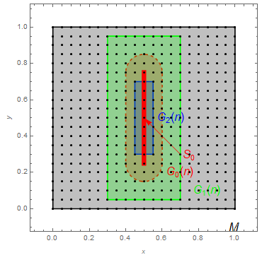
Figure 5: Illustration of the construction in Proposition 3.10 with the density in Figure 1. With $r=0.1$, the grid centers in $G(n)$ are displayed. The range of $G_{0}(n)$ is displayed in red; the ranges of $G_{1}(n)$ and $G_{2}(n)$ are displayed in green and blue, respectively.

Proof.

We consider the covering where the centers of the balls in $\mathcal{B}_{r(n)}^{2}(M)$ are exactly the grid set

$$G(n) =M\cap\{\boldsymbol{y}=(y_{1},y_{2})\in\mathbb{R}^{2}\mid y_{1},y_{2}\in\mathbb{N}\cdot\frac{r(n)}{2}\}.$$ (4)

(See Figure 5 for an illustration.) The cardinality of this covering is the same as the cardinality of the grid set $G(n)$. As $n$ increases, we have a sequence of coverings whose cardinalities are of order $O\left(\frac{1}{r(n)/2}\right)^{2}\sim O(n^{2\eta})$ as required in A.5.

Next, we prove that the covering balls of $\mathcal{B}_{r(n)}^{2}(M)$ intersecting $S_{0}$ also have cardinalities that satisfy A.6. Let $n$ be large enough that $r(n)<1/10$ and the $r(n)$-neighborhood of $S_{0}$, $B_{r(n)}(S_{0})\subset\text{int }M$. Consider the set of grids $G_{0}(n)\coloneqq\{\boldsymbol{y}=(y_{1},y_{2})\in G(n)\mid 0\leq d(\boldsymbol{y},S_{0})<r(n)\}$. A covering ball in $\mathcal{B}_{r(n)}^{2}(M)$ intersects $S_{0}$ if and only if its center is in $G_{0}(n)$. We construct the rectangular grids defined below to bound the cardinality of $G_{0}(n)$.

$\displaystyle G_{1}(n)\coloneqq$ $\displaystyle\{\boldsymbol{y}=(y_{1},y_{2})\in G(n)\mid\frac{1}{2}-2r(n)\leq y_{1}\leq\frac{1}{2}+2r(n),\frac{1}{4}-2r(n)\leq y_{2}\leq\frac{3}{4}+2r(n)\},$ $\displaystyle G_{2}(n)\coloneqq$ $\displaystyle\{\boldsymbol{y}=(y_{1},y_{2})\in G(n)\mid\frac{1}{2}-\frac{r(n)}{2}\leq y_{1}\leq\frac{1}{2}+\frac{r(n)}{2},\frac{1}{4}+\frac{r(n)}{2}\leq y_{2}\leq\frac{3}{4}-\frac{r(n)}{2}\}.$ It is clear from their definitions that $G_{2}(n)\subset G_{0}(n)\subset G_{1}(n)$.

In the grid set $G_{2}(n)$, there are at least $\frac{r(n)}{r(n)/2}=2$ grid points with the same value of $y_{2}$; and at least $\left\lfloor\frac{1/2-r(n)}{r(n)/2}\right\rfloor=\left\lfloor\frac{1}{r(n)}-2\right\rfloor$ points with the same value of $y_{1}$. Thus there are at least $2\cdot\left\lfloor\frac{1}{r(n)}-2\right\rfloor$ grid points in $G_{2}(n)$. Similarly, in the grid set $G_{1}(n)$ there are at most $\frac{4r(n)}{r(n)/2}+1=9$ grid points with the same value of $y_{2}$; and at most $\left\lceil\frac{1/2+4r(n)}{r(n)/2}+1\right\rceil=\left\lceil\frac{1}{r(n)}+9\right\rceil$ points with the same value of $y_{1}$. Thus there are at most $9\cdot\left\lceil\frac{1}{r(n)}+9\right\rceil$ grid points in $G_{2}(n)$.

Since $G_{2}(n)\subset G_{0}(n)\subset G_{1}(n)$, the number of balls intersecting $S_{0}$ has cardinality $\left|G_{0}(n)\right|$ bounded by the inequality

$$2\cdot\left\lfloor\frac{1}{r(n)}-2\right\rfloor\leq\left|G_{2}(n)\right|\leq\left|G_{0}(n)\right|\leq\left|G_{1}(n)\right|\leq 9\cdot\left\lceil\frac{1}{r(n)}+9\right\rceil.$$ (5)

Both sides of (5) have order of magnitude $O\left(\frac{1}{r(n)}\right)\sim O(n^{\eta})$ and this verifies A.6. ∎

Although we have shown by example that our Assumption A.1-A.6 can be verified for many densities, we point out that in general it might not be easy to verify these assumptions when $S_{0}$ or $M$ possesses a complicated topological structure.

3.2 Main result

Our main result connects coverings to data points. An “empty” ball centered at $\boldsymbol{x}$ is one for which $\{X_{1},\cdots,X_{n}\}\cap B_{r(n)}(\boldsymbol{x})=\emptyset$.

Theorem 3.11.

Suppose we have a set of i.i.d. data $X_{1},\cdots,X_{n}$ drawn from a continuous density $f(\boldsymbol{x})$ w.r.t. the $d$-dimensional Lebesgue measure $\nu^{d}$ defined on a compact subset $M=[0,1]^{d}$ of $\mathbb{R}^{d}$ and assume that Assumptions A.1-A.6 hold. Assume also that the radius $r$ and the separation distance $\epsilon$ satisfy the following growth rates:

$$r(n)\sim O(n^{-\eta}) ,\,0<\eta<\frac{1}{d},$$

$$\epsilon(n)\sim O(n^{-\psi}) ,\>0<\psi\leq\eta,$$

$$2r (n)\leq\epsilon(n)<1.$$

Finally, assume the validity of the following bounding condition for the density $f$ outside the $\epsilon$-neighborhood of $S_{0}$:

$$m(f,n)\coloneqq\min_{\boldsymbol{w}\in M\backslash B_{\epsilon}(S_{0})}f(\boldsymbol{w}) \in(0,\infty)\sim O(n^{-\xi}),\,0<\xi<\frac{1-2\eta d}{2}.$$

Then:
(A) If $\eta$ and $\psi$ satisfy

$$\begin{array}[]{c}1-2\eta d-2\overline{K_{f}}\psi>0,\end{array}$$

we have $\lim_{n\rightarrow\infty}P(\text{{\color[rgb]{0,0,0}there are no empty} $\epsilon$(n)-outside balls})=1$.

(B) If $\eta$ satisfies

$$\begin{array}[]{c}1+d_{0}\eta-\underline{K_{f}}\eta-d\eta<0,\end{array}$$

we have $\lim_{n\rightarrow\infty}P(\text{all $\epsilon$(n)-inside balls are empty})=1$.

The proof is given in Appendix A.

Similarly, we have a result dealing with the situation where $S_{0}$ has more than one (but a finite number) connected component.

Corollary 3.12.

Under the same assumptions as in Theorem 3.11, suppose that the zero-density region can be decomposed into $K$ disjoint connected components, $S_{0}=\sqcup_{k=1}^{K}S_{0k}$. For $n$ large enough (so that $\epsilon$ is small enough), an $\epsilon$-neighborhood of $S_{0}$ will also be comprised of $K$ disjoint connected components, the $\epsilon$-neighborhoods of each component $S_{0k}$.

Assume that the following bounding conditions for the density $f$ outside the $\epsilon$-neighborhood of each component $S_{0k}$ hold:

$$m_{k}(f,n)\coloneqq\min_{\boldsymbol{w}\in M\backslash B_{\epsilon(n)}(S_{0k})}f(\boldsymbol{w}) \in(0,\infty)\sim O(n^{-\xi}),\,0<\xi<\frac{1-2\eta d}{2}.$$

Assume also that the orders of smoothness of $f$ w.r.t. $S_{0k}$ are $\overline{K_{f,k}}$ and $\underline{K_{f,k}}>0$ and that, for $S_{0k}$ of dimension $d_{0k}$, the cardinality of the set of covering balls intersecting $S_{0k}$ is of order $O(n^{\eta d_{0k}})$.

Then:

(A) If $\eta$ and $\psi$ satisfy

$$\min_{k=1,\cdots,K}\begin{array}[]{c}1-2\eta d-2\overline{K_{f,k}}\psi>0,\end{array}$$

we have $\lim_{n\rightarrow\infty}P(\text{{\color[rgb]{0,0,0}there are no empty} $\epsilon$(n)-outside balls})=1$ for all $k$.

(B) If $\eta$ satisfies

$$\max_{k=1,\cdots,K}\begin{array}[]{c}1+d_{0k}\eta-\underline{K_{f,k}}\eta-d\eta<0,\end{array}$$

we have $\lim_{n\rightarrow\infty}P(\text{all $\epsilon$(n)-inside balls are empty})=1$ for all $k$.

4 Non-compact support

The main result of the previous section relies on the assumption of a compact support for the density $f$. However, in practice, many distributions have unbounded supports. In this section we consider the case of a density function $f$ with a non-compact support contained in $\mathbb{R}^{d}$ and, assuming that the tails of the density decay at certain rates, we derive results similar to those of the previous section.

Our strategy restricts our consideration to a region within the support that contains most of the probability mass of the density $f$. The original motivation for these ideas comes from the concentration inequalities that describe the fact that observations usually “concentrate” around the “center” of a probability density with high probability (for example, [30]).

Suppose that the support of the probability density function $f$ is a non-compact set $M^{{}^{\prime}}\subset\mathbb{R}^{d}$. We consider a truncation of the non-compact support $M^{{}^{\prime}}$ to a compact subset that contains most of the probability mass of $f$ and whose interior contains (all components of) $S_{0}$. This allows us to examine the topological features of $M^{{}^{\prime}}$ over a compact truncated region that contains the bulk of the data and to establish our results using arguments similar to those used to prove Theorem 3.11. For ease of exposition, we focus parts of our discussion on the situation where $M^{{}^{\prime}}=\mathbb{R}^{d}$, although most of our results can be extended to more general situations. We will state the restrictions on the tail behavior of the density functions in Proposition 4.9.

Definition 4.1.

($(1-\delta)$-support containing $S_{0}$) A $(1-\delta)$-support containing $S_{0}$ for some $0<\delta<1$, denoted by $S_{f}^{1-\delta}\subset\mathbb{R}^{d}$, is a subset of the form $S_{f}^{1-\delta}\coloneqq[-B,B]^{d}\subset\mathbb{R}^{d}$ for some $B\in(0,\infty)$, such that $S_{0}\subset\text{int }S_{f}^{1-\delta}=(-B,B)^{d}$ and $P\left\{X\in S_{f}^{1-\delta}\right\}=1-\delta$.

The hypercube $[-B,B]^{d}$ containing $1-\delta$ of the probability expands as $\delta$ shrinks. If $S_{0}$ is compact then $S_{f}^{1-\delta}$ exists for a small enough $\delta_{0}\in(0,1)$; if $S_{0}$ is non-compact, then it is unbounded and $S_{f}^{1-\delta}$ does not exist for any $\delta\in(0,1)$. For our subsequent results, we assume that the $(1-\delta)$-support is completely contained in the interior of the support $M^{{}^{\prime}}$.

Passing from $M^{{}^{\prime}}$ to $S_{f}^{1-\delta}$ allows us to work with a compact cubical subset and removes the technical difficulties associated with densities whose tails decay to zero. We replicate the results of Section 3 with modifications to Assumptions A.1-A.6. The modifications stem from replacing the compact support $[0,1]^{d}$ with a compact set $S_{f}^{1-\delta}$ that covers $S_{0}$ and contains $1-\delta$ mass of the probability measure.

We first consider the case where $\delta>0$ and $S_{f}^{1-\delta}$ are both fixed and state Assumptions A.1’-A.6’ for the non-compact support case.

1. Global assumptions on $f$, $M$, and $S_{0}$

   A.1’. (Non-compact support) The support of $f$ is $supp(f)=M^{{}^{\prime}}\subset\mathbb{R}^{d}$, $d>0$ and we consider the version of the density $f$ that is zero on $\mathbb{R}^{d}\backslash M^{{}^{\prime}}$ and continuous on $M^{{}^{\prime}}$.

   A.2’. (Single component) The zero-density region $S_{0}$ is contained in the interior of $M^{{}^{\prime}}$ and has one connected component.

2. Local assumptions on $f$ and $S_{0}$

   A.3’. (Order of smoothness) There exists an $\epsilon_{0}>0$ such that both quantities $\overline{K_{f}}(\epsilon_{0})>0$ and $\underline{K_{f}}(\epsilon_{0})>0$ exist.

   A.4’. Let $\epsilon_{0}>0$ be as described in A.3’. There exist two positive constants $L_{f}$ and $U_{f}$ such that, for all $\epsilon$ with $0<\epsilon<\min(1,\epsilon_{0})$, $L_{f}\cdot d(\boldsymbol{x},S_{0})^{\overline{K_{f}}(\epsilon)}\leq f(\boldsymbol{x})\leq U_{f}\cdot d(\boldsymbol{x},S_{0})^{\underline{K_{f}}(\epsilon)}$ for all $\boldsymbol{x}\in B_{\epsilon}(S_{0})\cap S_{f}^{1-\delta}$.

3. Assumptions on coverings

   A.5’. (Regular covering) There is an $\eta>0$ such that the elements of the sequence of coverings $\mathcal{B}_{r(n)}^{d}(S_{f}^{1-\delta})$ are comprised of balls whose centers lie in $\text{int }S_{f}^{1-\delta}$ and whose radii satisfy $r(n)\sim O(n^{-\eta})$. The sequence of coverings is regular, i.e., the cardinalities $|\mathcal{B}_{r(n)}^{d}(S_{f}^{1-\delta})|$ of the coverings in the sequence satisfy the condition $|\mathcal{B}_{r(n)}^{d}(S_{f}^{1-\delta})|\sim O(n^{d\eta})$.

   A.6’. (Restriction of covering to $S_{0}$) Let $\mathcal{B}_{r(n)}^{d}(S_{f}^{1-\delta})$ be the covering considered in A.5’. If $d_{0}$ is the Minkowski dimension of $S_{0}$ and $d_{0}<d$, then the number of balls in $\mathcal{B}_{r(n)}^{d}(S_{f}^{1-\delta})$ intersecting $S_{0}$ is bounded from above by $H_{\varepsilon}(n)\sim O(n^{d_{0}\eta(1+\varepsilon)})$, for each $\varepsilon>0$.

As for the compact case on page 3.8, these assumptions can be divided into three groups. A.1’ and A.2’ are restrictions on the topology on the support; A.3’ and A.4’ are descriptions of the local behavior of the density function; and A.5’ and A.6’ stipulate the existence of a sequence of coverings with good properties.

Theorem 4.2.

Consider a sequence of i.i.d. data $X_{1},X_{2}\cdots$ drawn from a distribution having a continuous density $f(\boldsymbol{x})$ w.r.t. the $d$-dimensional Lebesgue measure $\nu^{d}$ on $\mathbb{R}^{d}$. Assume that A.1’-A.6’ hold and that $S_{f}^{1-\delta}\subset\text{int }M^{{}^{\prime}}$. Assume also that the radius $r$ and the separation distance $\epsilon$ satisfy the following growth rates:

$$r(n)\sim O(n^{-\eta}) ,\,0<\eta<\frac{1}{d},$$

$$\epsilon(n)\sim O(n^{-\psi}) ,\,0<\psi\leq\eta,$$

$$2r (n)\leq\epsilon(n)<1.$$

Finally, assume that the density $f$ outside the $\epsilon$-neighborhood of $S_{0}$ satisfies:

$$m(f,n)\coloneqq\min_{\boldsymbol{w}\in S_{f}^{1-\delta}\backslash B_{\epsilon}(S_{0})}f(\boldsymbol{w}) \in(0,\infty)\sim O(n^{-\xi}),\,0<\xi<\frac{1-2\eta d}{2}.$$

Then:

(A) If $\eta$ and $\psi$ satisfy

$$\begin{array}[]{c}1-2\eta d-2\overline{K_{f}}\psi>0,\end{array}$$

we have $\lim_{n\rightarrow\infty}P(\text{{\color[rgb]{0,0,0}there are no empty }$\epsilon$(n)-outside balls})=1$.

(B) If $\eta$ and $\psi$ satisfy

$$\begin{array}[]{c}1+d_{0}\eta-\underline{K_{f}}\eta-d\eta<0,\end{array}$$

we have $\lim_{n\rightarrow\infty}P(\text{all $\epsilon$(n)-inside balls are empty})=1$.

Proof.

The idea of the proof is that the number of samples falling inside $S_{f}^{1-\delta}$ is close to the total number of samples, $n$, by the definition of $(1-\delta)$-support and the law of large numbers. By assumption, we know that $S_{f}^{1-\delta}$ is the hyper-cube $[-B,B]^{d}$ contained in $\text{int }M^{{}^{\prime}}$ and that A.1’-A.6’ hold. The number $n_{\delta}$ of observations that fall in $S_{f}^{1-\delta}$ has a $Binom(n,1-\delta)$ distribution. Using the two-sided Hoeffding inequality, (20) of the appendix, with $\gamma=\frac{\delta}{2},p=1-\delta$, we have:

$$P(n_{\delta}\geq n(1-\delta-\frac{\delta}{2})) =P(n_{\delta}\geq n(1-\frac{3\delta}{2}))$$

$$\geq P((1-\frac{3\delta}{2})n\leq n_{\delta}\leq(1-\frac{\delta}{2})n)$$

$$\geq 1-2\exp\left(-\frac{\delta}{2}^{2}n\right).$$

Conditioning on the event that that $n_{\delta}\geq n(1-\frac{3\delta}{2})$ merely adds a nonzero multiplicative factor to the probabilities of the events appearing in cases (A) and (B) of the statement of the theorem. With this adjustment the proof of this theorem parallels that of Theorem 3.11. The conditional probabilities of the events in (A) and (B) tend to 1 as $n\rightarrow\infty$. We also know that, as $n\rightarrow\infty$, the probability of the conditioning event tends to 1, completing the proof. ∎

The result above is stated for a fixed $(1-\delta)$-support $S_{f}^{1-\delta}$. As the sample size $n$ tends to infinity, we do not want to constrain ourselves to a fixed $S_{f}^{1-\delta}$, since this will prevent us from exploring the entire support of $f$. Consider a sequence of regions $S_{f}^{1-\delta(n)}$ with a decreasing sequence of $\delta=\delta(n)$, expanding the region under consideration as the sample accumulates. To retain the conclusions of the theorem, we must take care to expand the region slowly enough to control the decay of the density near the edges of $S_{f}^{1-\delta(n)}$.

In what follows, we denote by $\mathcal{B}_{r(n)}^{d}$ a covering of $S_{f}^{1-\delta(n)}$ and assume that A.5’ and A.6’ hold for this sequence of coverings. (Note that, here, $\mathcal{B}_{r(n)}^{d}$ denotes a covering of the $(1-\delta)$ support, not of $\mathbb{R}^{d}$, and that we dropped the explicit dependence on $S_{f}^{1-\delta(n)}$ that appears in A.5’ and A.6’ to simplify notation.)

Theorem 4.2 considers a fixed $\delta$. The upcoming theorems 4.3 and 4.4 allow $\delta$ to shrink toward $0$.

Theorem 4.3.

Under the assumptions of Theorem 4.2 (except for $\delta(n)$), consider a positive decreasing sequence $\delta(n)\,\text{satisfying }\lim_{n\rightarrow\infty}\delta(n)=0$ and the associated sequence of $(1-\delta)$-supports $S_{f}^{1-\delta(n)}$. For each $(1-\delta)$-support $S_{f}^{1-\delta(n)}$ we consider its corresponding covering $\mathcal{B}_{r(n)}^{d}$ consisting of open balls of radius $r(n)$.

Assume that

$$M(f)\coloneqq\sup_{\boldsymbol{w}\in\mathbb{R}^{d}}f(\boldsymbol{w}) \in(0,\infty),$$

$$m(f,n)\coloneqq\min_{\boldsymbol{w}\in S_{f}^{1-\delta(n)}\backslash B_{\epsilon(n)}(S_{0})}f(\boldsymbol{w}) \in(0,\infty)\sim O(n^{-\xi}),\,0<\xi<\frac{1-2\eta d}{2},$$

and that the cardinality $|\mathcal{B}_{r(n)}^{d}|\sim o(n^{\Omega}),\,\Omega\geq\eta>0$.

Then, if $\eta$ and $\psi$ satisfy

$$\begin{array}[]{c}1-2\eta d-2\overline{K_{f}}\cdot\psi>0,\end{array}$$

we have $\lim_{n\rightarrow\infty}P(\text{{\color[rgb]{0,0,0}there are no empty }$\epsilon$(n)-outside balls})=1$.

Proof.

We denote the number of total samples by $n$ and the number of samples falling inside $S_{f}^{1-\delta(n)}$ by $\mathcal{N}_{\delta(n)}$. To start, let us consider a sufficiently large $n\geq\mathsf{N}_{1}$ such that the decreasing sequence satisfies $\delta(n)\leq 0.1$ so that $1-\delta(n)\geq 0.9$. Then, let us decompose the event $C_{n}=\{\text{{\color[rgb]{0,0,0}there are no empty }$\epsilon(n)$-outside balls}\}$ using the event $D_{n}=\{0.95n\leq\mathcal{N}_{\delta(n)}\leq n\}$ and its complement. The the law of total probability yields:

$$P(C_{n}) =P(C_{n}\mid D_{n})\cdot P(D_{n})+P(C_{n}\mid D_{n}^{c})\cdot P(D_{n}^{c})$$

$$\geq P(C_{n}\mid D_{n})\cdot P(D_{n}).$$ (6)

The event $D_{n}$ involves a binomial random variable $\mathcal{N}_{\delta(n)}$, therefore $P(D_{n})$ can be bounded by the Hoeffding inequality, (20) of the appendix. Since $1-\delta(n)\geq 0.9$,

$$P(D_{n})=P(0.95n \leq\mathcal{N}_{\delta(n)}\leq n)\geq 1-2\exp\left(-\frac{0.1}{2}^{2}n\right).$$ (7)

The other term, $P(C_{n}\mid D_{n})$, can also be bounded by the following argument. (Note that $r(n)$ and $\epsilon(n)$ only depend on the total sample size $n$, not on $\mathcal{N}_{\delta(n)}$.)

$$P(C_{n}\mid D_{n}) =1-P(C_{n}^{c}\mid D_{n})$$

$$\geq 1-\sum_{B\in\{\epsilon(n)-\text{outside balls}\}}P(B\text{ empty}\mid D_{n})$$

$$\geq 1-|\mathcal{B}_{r(n)}^{d}|\cdot\left(1-\inf_{B\in\{\epsilon(n)-\text{outside balls}\}}P(B\text{ not empty}\mid D_{n})\right).$$ (8)

By the bound in (22) in the proof of Theorem 3.11 in the appendix and the assumption that $|\mathcal{B}_{r(n)}^{d}|\sim o(n^{\Omega})$ we have

$$|\mathcal{B}_{r(n)}^{d}|\cdot\left(1-\inf_{B\in\{\epsilon(n)-\text{outside balls}\}}P(B\text{ not empty}\mid D_{n})\right)\sim$$

$$o(n^{\Omega})\cdot O\left(\exp\left(-n^{\min(1-2\eta d-2\overline{K_{f}}\cdot\psi,1-2\eta d-2\xi)}\right)\right),$$

which is monotonically decreasing since $\min(1-2\eta d-2\overline{K_{f}}\cdot\psi$ ) $>0$ and $\xi<\frac{1-2\eta d}{2}$ by the assumptions of the theorem.Using the definition of big/small O notation, we can find a constant $L\in(0,\infty)$ such that

$$P(C_{n}\mid D_{n}) \geq 1-L\cdot n^{\Omega}\cdot\exp\left(-n^{1-2\eta d-2\overline{K_{f}}\cdot\psi}\right)\text{ for sufficiently large }n.$$ (9)

The bounds (7) and (9) can be substituted back into (6) to obtain

$$P(C_{n}) \geq P(C_{n}\mid D_{n})\cdot P(D_{n})$$

$$\geq\left(1-L\cdot n^{\Omega}\cdot\exp\left(-n^{1-2\eta d-2\overline{K_{f}}\cdot\psi}\right)\right)\left(1-2\exp\left(-\frac{0.1}{2}^{2}n\right)\right).$$ (10)

As long as $1-2\eta d-2\overline{K_{f}}\cdot\psi>0$, this lower bound tends to 1 as $n$ goes to infinity. ∎

It is important to notice that it is the decay rates of $m(f,n)$ and $|\mathcal{B}_{r(n)}^{d}|\sim o(n^{\Omega})$ that determine the sufficient conditions of Theorem 4.3, not the rate at which the volume of $S_{f}^{1-\delta(n)}$ increases.

The following theorem deals with the $\epsilon(n)$-inside balls.

Theorem 4.4.

Under the assumptions of Theorem 4.2 (except for $\delta(n)$), consider a positive decreasing sequence $\delta(n)\,\text{satisfying }\lim_{n\rightarrow\infty}\delta(n)=0$ and the associated sequence of $(1-\delta)$-supports $S_{f}^{1-\delta(n)}$. For each $(1-\delta)$-support $S_{f}^{1-\delta(n)}$ we consider its corresponding covering $\mathcal{B}_{r(n)}^{d}$ consisting of open balls of radius $r(n)$.

Assume that

$$m(f,n)\coloneqq\min_{\boldsymbol{w}\in S_{f}^{1-\delta(n)}\backslash B_{\epsilon(n)}(S_{0})}f(\boldsymbol{w}) \in(0,\infty)\sim O(n^{-\xi}),\,0<\xi<\frac{1-2\eta d}{2}.$$

Then, if $\eta$ and $\psi$ satisfy

$$\begin{array}[]{c}1+d_{0}\eta-\underline{K_{f}}\eta-d\eta<0,\end{array}$$

we have $\lim_{n\rightarrow\infty}P(\text{all $\epsilon$(n)-inside balls are empty})=1$.

Proof.

This result can be established by following exactly the same proof as that for case (B) in Theorem 4.2. Since $S_{0}\subset\text{int }M^{\prime}$ we can choose $\mathsf{N}_{1}$ sufficiently large so that $B_{\epsilon(n)}(S_{0})\subset\text{int }S_{f}^{1-\delta(n)}$, for $n\geq\mathsf{N}_{1}$. The probability of the event that an individual $\epsilon(n)$-inside ball is empty does not depend on the varying sequence of regions $S_{f}^{1-\delta(n)}$. For an appropriate $\mathsf{N}_{2}$ and every $n\geq\mathsf{N}_{2}$, our assumption A.6’ restricts the number of $\epsilon$-inside balls and this cardinality does not depend on the varying $(1-\delta(n))$-supports. The rest of the proof parallels that of Theorem 4.2 (B), considering $n\geq\max(\mathsf{N}_{1},\mathsf{N}_{2})+1$. ∎

The existence of a sequence of $\delta(n)$ values satisfying the above conditions can be verified for densities exhibiting specific tail behaviors on their supports. Two examples of such densities are given in the two examples following Definitions 4.5 and 4.7 and are depicted in Figure 6.

Definition 4.5.

(Polynomial tail) We say that a continuous density $f$ supported on $\mathbb{R}^{d}$ has a polynomial tail if it has the form

$$f(\boldsymbol{x})=\begin{cases}f_{1}(d(\boldsymbol{x},S_{0}))=C_{1}\cdot d(\boldsymbol{x},S_{0})^{\gamma},&d(\boldsymbol{x},S_{0})<\epsilon_{0},\\ f_{2}(d(\boldsymbol{x},S_{0}))=C_{2}\cdot d(\boldsymbol{x},S_{0})^{\chi},&d(\boldsymbol{x},S_{0})\geq\epsilon_{0},\end{cases}$$ (11)

for some $C_{1},C_{2}\in(0,\infty)$, $\gamma>0$, and $\chi<-d$. Note that the continuity assumption on the density $f$ requires $C_{1}\cdot\epsilon_{0}^{\gamma}=C_{2}\cdot\epsilon_{0}^{\chi}$.

Example 4.6.

Consider a continuous density $f$ of the form (11) with $d=1,\,S_{0}=\{0\},\,\epsilon_{0}=1,\,\gamma=\frac{1}{3},\,\text{and }\chi=-2$, leading to the density

$$f(x)=\begin{cases}\frac{2}{7}\cdot|x|^{1/3},&|x|<1,\\ \frac{2}{7}\cdot|x|^{-2},&|x|\geq 1,\end{cases}.$$

This density yields $\frac{2}{7}\int_{-1}^{1}|x|^{1/3}dx=\frac{3}{7}$. We can take $n$ sufficiently large so that $\delta(n)<\frac{4}{7}$. From the definition of $(1-\delta(n))$-support we have $B(n)>\epsilon_{0}=1$ for $\delta(n)<\frac{4}{7}$. The defining equation of $B(n)$ is $\int_{-\infty}^{-B(n)}f(x)dx+\int_{B(n)}^{\infty}f(x)dx=2\int_{B(n)}^{\infty}f(x)dx=\delta(n).$ Therefore $B(n)=\frac{1}{\frac{7}{4}\delta(n)}\sim O(\delta(n)^{-1})$.

The maximum of this density function is attained at $x=\pm 1$ and equals $M(f)=\frac{2}{7}$. Let $\xi$ and $\psi$ be as defined in Theorem 4.2. Then, if we choose sequences $\delta(n)\sim O(n^{\xi/\chi})\sim O(n^{-\xi/2})$ and $\text{$\epsilon(n)$}\sim O(n^{-\psi})\sim O(n^{-\xi/\gamma})\sim O(n^{-3\xi})$, we will ensure that the minimal value $m(f,n)\coloneqq\min_{\boldsymbol{w}\in S_{f}^{1-\delta(n)}\backslash B_{\epsilon(n)}(S_{0})}$ $f(\boldsymbol{w})=$ $\min\left(C_{1}\cdot\epsilon(n)^{\gamma},C_{2}\cdot B(n)^{\chi}\right)=\min\left(\frac{2}{7}\epsilon(n)^{1/3},\frac{2}{7}B(n)^{-2}\right)$. We have $\frac{2}{7}\epsilon(n)^{1/3}$ $\sim O(n^{-\xi})$ and $\frac{2}{7}B(n)^{-2}\sim O(n^{-\xi})$, so that $m(f,n)\sim O(n^{-\xi})$. Furthermore, $\delta(n)\sim O(n^{-\xi/2})\rightarrow 0$. The assumptions on the density function in Theorem 4.2 are therefore satisfied.

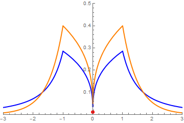
Figure 6: Density functions with polynomial tails (blue) and exponential tails (orange).

Definition 4.7.

(Exponential tail) We say that a continuous density $f$ supported on $\mathbb{R}^{d}$ has an exponential tail if it has the form

$$f(\boldsymbol{x})=\begin{cases}f_{1}(d(\boldsymbol{x},S_{0}))=C_{1}\cdot d(\boldsymbol{x},S_{0})^{\gamma},&d(\boldsymbol{x},S_{0})<\epsilon_{0},\\ f_{2}(d(\boldsymbol{x},S_{0}))=C_{2}\cdot\exp(\beta d(\boldsymbol{x},S_{0})),&d(\boldsymbol{x},S_{0})\geq\epsilon_{0},\end{cases}$$ (12)

for some $C_{1},C_{2}\in(0,\infty)$, $0<\gamma$ and $\beta<0$. Note that the continuity assumption on the density $f$ requires $C_{1}\cdot\epsilon_{0}^{\gamma}=C_{2}\cdot\exp(-\beta\epsilon_{0})$.

Example 4.8.

Consider a continuous density $f$ of the form (12) with $d=1,\,S_{0}=\{0\},\,\epsilon_{0}=1,\,\gamma=\frac{1}{3},\,\text{and }\beta=-2$, leading to the density

$$f(x)=\begin{cases}\frac{2}{5}\cdot|x|^{1/3},&|x|<1,\\ \frac{2}{5}\cdot e^{2}\cdot e^{-2|x|},&|x|\geq 1,\end{cases}.$$

This density yields $\int_{-1}^{1}\frac{2}{5}\cdot|x|^{1/3}dx=\frac{3}{5}$. We can take $n$ sufficiently large so that $\delta(n)<\frac{2}{5}$. From the definition of $(1-\delta(n))$-support we have $B(n)>\epsilon_{0}=1$ for $\delta(n)<\frac{2}{5}$. The defining equation of $B(n)$ is $\int_{-\infty}^{-B(n)}f(x)dx+\int_{B(n)}^{\infty}f(x)dx=2\int_{B(n)}^{\infty}f(x)dx=\delta(n).$ Therefore $B(n)=1-\frac{1}{2}\log\left(1+\frac{5}{2}\delta(n)\right)\sim O(-\log\delta(n))$.

The maximum of this density function is attained at $x=\pm 1$ and equals $M(f)=\frac{2}{5}$. Let $\xi$ and $\psi$ be as defined in Theorem 4.2. Then if we choose sequences $\delta(n)\sim O(n^{\xi/\beta})\sim O(n^{-\xi/2})$ and $\text{$\epsilon(n)$}\sim O(n^{-\psi})\sim O(n^{-\xi/\gamma})\sim O(n^{-3\xi})$, we will ensure that the minimal value $m(f,n)\coloneqq\min_{\boldsymbol{w}\in S_{f}^{1-\delta(n)}\backslash B_{\epsilon(n)}(S_{0})}f(\boldsymbol{w})=\min\left(C_{1}\cdot\epsilon(n)^{\gamma},C_{2}\cdot\exp(\beta B(n))\right)$
$=\min\left(\frac{2}{5}\epsilon(n)^{1/3},\frac{2}{5}e^{2}\cdot\exp\left(-2B(n)\right)\right)$. We have $\frac{2}{5}\epsilon(n)^{1/3}\sim O(n^{-\xi})$ and $\frac{2}{5}e^{2}\cdot\exp\left(-2B(n)\right)\sim O(n^{-\xi})$, so that $m(f,n)\sim O(n^{-\xi})$. Furthermore, $\delta(n)\sim O(n^{-\xi/2})\rightarrow 0$. The assumptions on the density function in Theorem 4.2 are therefore satisfied.

The essence of the examples above is embodied in the following general result whose proof follows along the path suggested by the examples.

Proposition 4.9.

Assume that a continuous density supported on $\mathbb{R}^{d}$ is of the form (11) or (12) with a compact zero-density region $S_{0}$. For fixed $0<\eta<\frac{1}{d},\,0<\xi<\frac{1-2\eta d}{2}$, we can find a sequence $\epsilon(n)\sim O(n^{-\psi}),\,0<\psi\leq\eta$, and a decreasing sequence of $\delta(n)$, with $\lim_{n\rightarrow\infty}\delta(n)=0$, such that

$$M(f) \coloneqq\sup_{\boldsymbol{w}\in\mathbb{R}^{d}}f(\boldsymbol{w})\in(0,\infty),$$

$$m(f,n)\coloneqq\min_{\boldsymbol{w}\in S_{f}^{1-\delta(n)}\backslash B_{\epsilon(n)}(S_{0})}f(\boldsymbol{w}) \in(0,\infty)\sim O(n^{-\xi}),\,0<\xi<\frac{1-2\eta d}{2}.$$

Proof.

That $M(f)\coloneqq\sup_{\boldsymbol{w}\in\mathbb{R}^{d}}f(\boldsymbol{w})\in(0,\infty)$ is a direct consequence of the assumptions about the form of (11) or (12).

We want to show that we can construct a decreasing sequence $\delta(n),$ with $\lim_{n\rightarrow\infty}\delta(n)=0$, such that the corresponding $1-\delta(n)$ supports $S_{f}^{1-\delta(n)}\coloneqq[-B(n),B(n)]^{d}$ have minimal values $m(f,n)\sim O(n^{-\xi})$. First, we choose the sequences $B(n)$ and $\epsilon(n)$, which jointly determine the desired decay rate of $m(f,n)$. Then, if $B(n)$ is an increasing sequence, by the definition of $S_{f}^{1-\delta(n)}$ as a cube, $\delta(n)$ is automatically a decreasing sequence.

To determine $B(n)$, we use a sandwich argument on the minimal value $m(f,n)$ attained on $S_{f}^{1-\delta(n)}$. We will consider two sequences of balls, one where each ball is contained in $S_{f}^{1-\delta(n)}$, called the sequence of inner tangential balls $\mathcal{B}_{*}(n)$, and the other where each ball contains $S_{f}^{1-\delta(n)}$, called the sequence of outer inclusive balls $\mathcal{B}^{*}(n)$:

$$\mathcal{B}_{*}(n) \coloneqq B_{B(n)}(\boldsymbol{0})\equiv\{\boldsymbol{x}\in\mathbb{R}^{d}\mid d(\boldsymbol{x},\boldsymbol{0})<B(n)\},$$ (13)

$$\mathcal{B}^{*}(n) \coloneqq B_{4\sqrt{d}B(n)}(\boldsymbol{0})\equiv\{\boldsymbol{x}\in\mathbb{R}^{d}\mid d(\boldsymbol{x},\boldsymbol{0})<4\sqrt{d}B(n)\}.$$ (14)

Consider the following minimal values of $f$ on $\mathcal{B}_{*}(n)\backslash B_{\epsilon(n)}(S_{0})$ and $\mathcal{B}^{*}(n)\backslash B_{\epsilon(n)}(S_{0})$,

$$m_{*}(f,n) =\inf_{\boldsymbol{w}\in\mathcal{B}_{*}(n)\backslash B_{\epsilon(n)}(S_{0})}f(\boldsymbol{w}),$$

$$m^{*}(f,n) =\inf_{\boldsymbol{w}\in\mathcal{B}^{*}(n)\backslash B_{\epsilon(n)}(S_{0})}f(\boldsymbol{w}).$$

Since $\mathcal{B}_{*}(n)\subset S_{f}^{1-\delta(n)}\subset\mathcal{B}^{*}(n)$ by the above construction, we have $m_{*}(f,n)\geq m(f,n)\geq m^{*}(f,n)$. When $f$ is of the form (11) or (12), we can choose the sequence $\epsilon(n)=\left(\frac{1}{C_{1}}\cdot n^{-\xi}\right)^{1/\gamma_{1}}$ where $\gamma_{1}\geq\gamma>0$ such that $0<\frac{\xi}{\gamma_{1}}\leq\eta$. We use this choice of $\epsilon(n)$ to ensure that $\epsilon(n)\sim O(n^{-\psi})\sim O(n^{-\frac{\xi}{\gamma_{1}}})$, and $0<\psi\leq\eta$ hold. Note that $\epsilon(n)$ is a decreasing sequence by definition.

(Polynomial tail) When $f$ is of the form (11), we use the $\epsilon(n)$ above and choose another sequence $B(n)=\left(\frac{1}{C_{2}}\cdot n^{\xi}\right)^{-1/\chi}$ and take $n$ sufficiently large so that $\epsilon(n)<\frac{1}{4}B(n)$ and $\epsilon_{0}<B(n)$. Then the minimal values for $\mathcal{B}_{*}(n)$ satisfy

$$m_{*}(f,n) \leq\min\left(C_{1}\cdot\epsilon(n)^{\gamma},C_{2}\cdot(B(n)-\epsilon(n))^{\chi},C_{2}\cdot B(n)^{\chi}\right)$$

$$\sim O\left(\min\left(C_{1}\cdot\epsilon(n)^{\gamma},C_{2}\cdot B(n)^{\chi}\right)\right)$$

$$\sim O\left(\min\left(C_{1}\cdot n^{-\frac{\gamma}{\gamma_{1}}\xi},n^{-\xi}\right)\right).$$

Since $\gamma/\gamma_{1}\leq 1$ for $n>1$ large enough, we have that this asymptotic order of magnitude is determined by the behavior of the second term and $m_{*}(f,n)\sim O(n^{-\xi})$. Similarly, the minimal values for $\mathcal{B}^{*}(n)$ satisfy

$$m^{*}(f,n) \geq\min\left(C_{1}\cdot\epsilon(n)^{\gamma},C_{2}\cdot(4\sqrt{d}B(n)+\epsilon(n))^{\chi}\right)$$

$$\sim O\left(\min\left(C_{1}\cdot\epsilon(n)^{\gamma},C_{2}\cdot B(n)^{\chi}\right)\right)$$

$$\sim O(n^{-\xi}).$$

(Exponential tail) When $f$ is of the form (12), we use the $\epsilon(n)$ above and choose another sequence $B(n)=\frac{1}{\beta}\log\left(\frac{1}{C_{2}}\cdot n^{-\xi}\right)$ and take $n$ sufficiently large so that $\epsilon(n)<\frac{1}{4}B(n)$ and $\epsilon_{0}<B(n)$. Then the minimal values for $\mathcal{B}_{*}(n)$ satisfy

$$m_{*}(f,n) \leq\min\left(C_{1}\cdot\epsilon(n)^{\gamma},C_{2}\cdot\exp(\beta(B(n)-\epsilon(n)))\right)$$

$$\sim O\left(\min\left(C_{1}\cdot\epsilon(n)^{\gamma},C_{2}\cdot\exp(\beta B(n))\right)\right)$$

$$\sim O\left(\min\left(C_{1}\cdot n^{-\frac{\gamma}{\gamma_{1}}\xi},n^{-\xi}\right)\right).$$

Since $\gamma/\gamma_{1}\leq 1$ for $n>1$ large enough, we have that this asymptotic order of magnitude is determined by the behavior of the second term and $m_{*}(f,n)\sim O(n^{-\xi})$. Similarly, the minimal values for $\mathcal{B}^{*}(n)$ satisfy

$$m^{*}(f,n) \geq\min\left(C_{1}\cdot\epsilon(n)^{\gamma},C_{2}\cdot\exp(\beta(4\sqrt{d}B(n)+\epsilon(n)))\right)$$

$$\sim O\left(\min\left(C_{1}\cdot\epsilon(n)^{\gamma},C_{2}\cdot\exp\left(\beta B(n)\right)\right)\right)$$

$$\sim O(n^{-\xi}).$$

By a sandwich argument with $\mathcal{B}_{*}(n)\subset S_{f}^{1-\delta(n)}\subset\mathcal{B}^{*}(n)$ and $m_{*}(f,n)\geq m(f,n)\geq m^{*}(f,n)$, we know that we can find some $\frac{1}{4\sqrt{d}}\cdot\left(\frac{1}{C_{2}}\cdot n^{\xi}\right)^{-1/\chi}\leq B(n)\leq\left(\frac{1}{C_{2}}\cdot n^{\xi}\right)^{-1/\chi}$ for a density of the form (11) or some $\frac{1}{4\sqrt{d}}\cdot\frac{1}{\beta}\log\left(\frac{1}{C_{2}}\cdot n^{-\xi}\right)\leq B(n)\leq\frac{1}{\beta}\log\left(\frac{1}{C_{2}}\cdot n^{-\xi}\right)$ for a density of the form (12). This choice of an increasing sequence of $B(n)$ proves our claim that we can find a sequence of $\delta(n),\,\text{with }\lim_{n\rightarrow\infty}\delta(n)=0$, such that $M(f)\in(0,\infty)$ and $m(f,n)\sim O(n^{-\xi})$. ∎

Corollary 4.10.

Consider a continuous density supported on $\mathbb{R}^{d}$ of the form (11) or (12). We can find a sequence $\epsilon(n)\sim O(n^{-\psi}),\,0<\psi\leq\eta$, and a decreasing sequence of $\delta(n)$ values, with $\lim_{n\rightarrow\infty}\delta(n)=0$, such that the associated sequence of $(1-\delta(n))$-supports $S_{f}^{1-\delta(n)}$ have corresponding coverings $\mathcal{B}_{r(n)}^{d}$ satisfying A.5’ and A.6’. Then

(A) If $\eta$ and $\psi$ satisfy

$$\begin{array}[]{c}1-2\eta d-2\overline{K_{f}}\cdot\psi>0,\end{array}$$

we have $\lim_{n\rightarrow\infty}P(\text{{\color[rgb]{0,0,0}there are no empty }$\epsilon$(n)-outside balls})=1$.

(B) If $\eta$ and $\psi$ satisfy

$$\begin{array}[]{c}1+d_{0}\eta-\underline{K_{f}}\eta-d\eta<0,\end{array}$$

we have $\lim_{n\rightarrow\infty}P(\text{all $\epsilon$(n)-inside balls are empty})=1$.

Proof.

By the result in Proposition 4.9, it suffices to consider the grid construction in Lemma 3.9. The cardinality of the resulting coverings $\mathcal{B}_{r(n)}^{d}$ of $S_{f}^{1-\delta(n)}$ can be guaranteed to be $O\left(\frac{B(n)^{d}}{r(n)^{d}}\right)$. So, for case (11) we can have $\left|\mathcal{B}_{r(n)}^{d}\right|\sim$
$O\left(\left(\frac{1}{C_{2}}\cdot n^{-\xi}\right)^{d/\chi}\cdot n^{\eta d}\right)$ and for case (12) we can have $\left|\mathcal{B}_{r(n)}^{d}\right|\sim$
$O\left(\frac{1}{\beta^{d}}\log^{d}\left(\frac{1}{C_{2}}\cdot n^{-\xi}\right)\cdot n^{\eta d}\right)$. In either case, $\left|\mathcal{B}_{r(n)}^{d}\right|$ is obviously $o(n^{\Omega})$ for some sufficiently large $\Omega>0$. Therefore all assumptions in Theorems 4.3 and 4.4 are met. ∎

5 Simulations and Connections to Other Areas

5.1 Simulation Studies for the choice of $r,\epsilon$

Our theoretical results establish the rate of decay for the radius $r(n)$ and the neighborhood width $\epsilon(n)$. That is, for any positive constants $M_{r}$ and $M_{\epsilon}$,

$$r(n) =M_{r}\cdot O(n^{-\eta}),$$

$$\epsilon(n) =M_{\epsilon}\cdot O(n^{-\psi}).$$

(with $\eta$ and $\psi$ following the same notation used in Theorem 3.11) the asymptotic guarantees of filled and empty balls hold. These guarantees allow one to identify lower dimensional zero-density regions in the limit. However, for a fixed sample size, the actual values of $r(n)$ and $\epsilon(n)$ matter. This subsection reports simulations investigating choice of the constants $M_{r}$ and $M_{\epsilon}$.

We consider the density $f(\boldsymbol{x})\propto d(\boldsymbol{x},S_{0})^{4}\circ\boldsymbol{1}_{[0,1]^{2}}$. The zero-density region $S_{0}=\{\frac{1}{2}\}\times[0.25,0.75]$ is of strictly lower dimension. For this example, $m(f,n)$ decays as a polynomial with $\xi=4\cdot\psi$ and $M(f)<2$. The conditions of Theorem 3.11, parts (A) and (B), hold with, for example, $\eta=0.21$ and $\psi=0.01$ (therefore $0<\xi\leq\frac{1-4\eta}{2}$).

In the simulation, random samples of various sizes are generated from the density. A grid of balls with centers on a lattice is used to cover the unit square. The centers of the balls depend on $M_{r}$ and $n$ and follow the rule we described in Proposition 3.10. We note that the fraction of filled balls of a particular kind serves as an empirical estimate of the mean probability that a particular kind of ball is non-empty.

Figure 7 presents the results of the simulation. The color scheme is the same as in Figure 4. Proceeding down a column, the sample size changes from 100 to 10,000. Tracking the red lines, we see that the percentage of filled $\epsilon$-inside balls tends to $0$ as $n$ increases. The orange lines represent the $\epsilon$-neighboring balls. The percentage of these that are filled does not always tend to $0$. The green lines represent the $\epsilon$-outside balls. Here, the fraction filled increases toward the eventual limit of $1$.

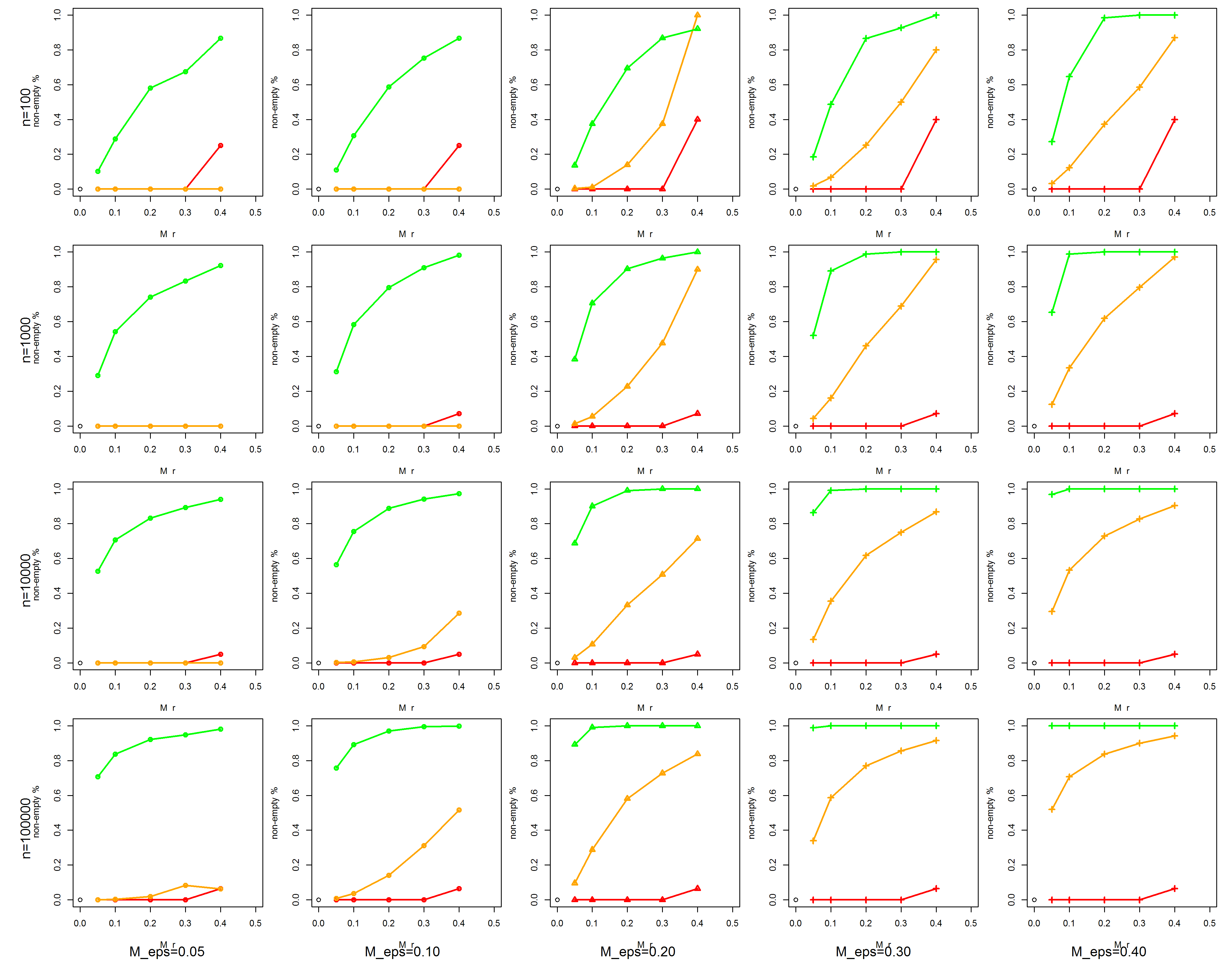
Figure 7: The percentage of various types of non-empty covering balls under different multipliers $M_{r}$ and $M_{\epsilon}$ for ball radius $r(n)$ of the covering and neighborhood width of $S_{0}$, $\epsilon(n)$, for various sample sizes $n$.

As we step across rows of the figure, the value of $M_{\epsilon}$ increases from $0.05$ to $0.40$. Within a plot, the value of $M_{r}$ increases from $0.05$ to $0.40$. As $r(n)$ increases, the balls are larger and a greater fraction are filled, as evidenced by the lines within each plot. As $M_{\epsilon}$ increases, balls in the covering are moved from $\epsilon$-outside to $\epsilon$-neighboring to $\epsilon$-inside. The changing values of $\epsilon(n)$ and $r(n)$ shuffle the group membership of the balls and change the resulting fractions. In general, the larger values of $M_{r}$ that we have investigated lead to greater separation of the red and green lines–hence greater differentiation between $\epsilon$-inside and $\epsilon$-outside balls. Larger values of $M_{\epsilon}$ have a similar, though weaker effect.

The simulation also provides a caution. The plots toward the bottom of the figure show much greater separation between the red and green lines. This separation (near 0, near 1) is needed in order to reliably detect a zero-density region. For this density, the larger sample sizes prove much more effective than do the smaller sample sizes.

The simulation results suggest an interesting possibility—the use of multiple coverings with balls of different sizes. Doing so could allow one to examine the set of $M_{r}$, $M_{\epsilon}$ pairs that suggest the presence of a zero-density region. In practice, when $n$ is finite, the choice of multipliers $M_{r}$ and $M_{\epsilon}$ impacts the results.

5.2 Connections to Existing Research

Our object of interest in this paper is the inverse image of $\{0\}$ under the continuous density function $f$, when it is of lower dimension than the support of $f$.

The lower dimensional zero-density region is of interest to the topological data analysis (TDA) research community. Topological data analysis methods have been developed to explore and understand the topological structure of the space where the data arise (for example, the support of a probability distribution) using a finite amount of observed data, as introduced in [5] and [11].

Having the data in hand, it is quite natural to consider them as a random sample from some probability distribution. Interest then focuses on the limiting behavior of geometric complexes based on a point set of growing size. In this regard, [16] and [17] have developed results about the limiting behavior of Betti numbers of complexes, based on the probabilistic results for random geometric graphs given by [25]. Subsequent work in this direction characterizes other types of topological features [10, 2, 18]. These results provide a picture of how the probability mechanism informs us about the underlying topology. [3] provide a comprehensive review of the results along this line. This body of literature suggests that asymptotic regimes provide a convenient framework for analyzing the topology of data, as we do in the current paper.

Another line of relevant literature is on the set estimation, [8], [27], and [29] study the related concept of the $\lambda$-level set for density $f$. That is, the set $S_{\lambda}\coloneqq\left\{\boldsymbol{x}\in\mathbb{R}^{d}\mid f(\boldsymbol{x})\geq\lambda\right\},\leavevmode\nobreak\ \lambda>0$. The special case where $\lambda=0$ is studied in [9]. The difference between the regions is that $S_{\lambda}$ is the inverse image of an open set that contains positive mass if non-empty while $S_{0}\coloneqq\left\{\boldsymbol{x}\in\mathbb{R}^{d}\mid f(\boldsymbol{x})=0\right\}$ is the inverse image of a closed set and contains no mass. To the best of our knowledge, regions like $S_{0}$ have not previously been studied.

In the level set estimation literature, there are two major approaches to the problem of estimating level sets. Suppose we are interested in estimating the level sets of density $f$ (corresponding to a probability measure $F$). One approach is to construct plug-in estimators $\hat{S_{\lambda}}\coloneqq\left\{\boldsymbol{x}\in\mathbb{R}^{d}\mid\hat{f}(\boldsymbol{x})>\lambda\right\}$ for a level set, based on a kernel density estimator $\hat{f}$ computed from the data and appropriate choices of the bandwidth parameters for the kernel [27, 23, 28]. This approach connects to the topology of the density when the level, $\lambda$, is varied [7, 13]. Asymptotically, a consistent estimator of the density may reveal persistent features.

The other approach is based on the empirical excess-mass functional. The (empirical) excess-mass functional $E(\lambda)\coloneqq F(S_{\lambda})-\lambda\text{Leb}(S_{\lambda})$ measures how the “excess probability mass” of the probability measure $F$ distributes over the region $S_{\lambda}$ when compared to Lebesgue measure [15]. If we substitute the set $S_{\lambda}$ with a set estimator $\hat{S_{\lambda}}$ for the $\lambda$-level set $S_{\lambda}$, we can similarly consider the functional $H(\lambda)\coloneqq F(\hat{S_{\lambda}})-\lambda\text{Leb}(\hat{S_{\lambda}})$, which can be used to evaluates the estimator $\hat{S_{\lambda}}$. The functional $H$ is maximized over a class of sets to obtain the level set estimator $\hat{S_{\lambda}}$ [26, 31], to obtain level set estimators $\hat{S_{\lambda}}$. The consistency and asymptotic behavior of both approaches has been derived under regularity assumptions.

In this paper, we study the lower dimensional object that arises as the inverse image of the density function $f$ of a single point set. When we restrict our concern to the manifold $supp(f)$ and the inverse of the density function $f^{-1}$ is sufficiently smooth, $f^{-1}(\{a\}),\,f^{-1}(\{b\})$ encode the boundary of the manifold defined by the inverse image $f^{-1}((a,b))$, as a sub-manifold of $supp(f)$. When $a=\lambda$ and $b=\infty$, this inverse image defines $\lambda$-level sets. The object $S_{0}=f^{-1}(\{0\})$ is the boundary of such a particular example where $a=0$ and $b=\infty$. Unlike the topological features associated with the level sets, the feature we study does not necessarily generate equivalent classes in (persistent) homology. However, in applications like image segmentation, the boundaries are features of major interest [21].

Our method detects this specific kind of lower dimensional topological feature that could arise as a manifold boundary. We construct a sequence of covering families to detect $S_{0}$ and we derive a set of sufficient conditions that ensure consistent detection in an asymptotic sense. As is to be expected, when more sample points are available, our covering scheme locates the zero-density region $S_{0}$ more accurately. In applied scenarios where the boundaries arise as zero-density regions of certain density functions, our method could help in detection [21].

We do not provide an estimator of $S_{0}$ in this paper. A referee suggested that the union of empty balls in a covering could constitute an estimator of $S_{0}$. Additionally, if $M$ were not known, the same referee suggested that our method could be applied to a preliminary estimate of $M$. This is an interesting direction, but it is too difficult to develop fully in this article. For one thing, the performance of the method would depend on the accuracy of the preliminary estimator. In addition, the theoretical properties of the method would become more intricate, owing to the dependence between the preliminary estimation of $M$ and the covering procedure.

The main results in this paper also exhibit the relation between topological features that arise as $S_{0}$, and its dimensionality. In [1] and [24], the authors observe that higher dimensional topological features are generally smaller in scale. As shown by the sufficient conditions in Theorem 3.11 and 4.2, when the dimension $d_{0}$ of $S_{0}$ is higher, we need to specify a faster decay rate for radii $r(n)$ of the covering sequence in order to meet the sufficient conditions. This interplay between the dimension of the support, the dimension of the zero-density region $S_{0}$ and the sufficient growth rates supports [1]’s observation from a different angle.

6 Conclusions

In this paper, we consider the question of detection of $S_{0}=f^{-1}(\{0\})$ lying in the support $M$ of a continuous density $f$ when $S_{0}$ has Minkowski dimension strictly lower than the dimension of the data, $d$. This type of topological feature is difficult to identify and has not been studied before. The main contribution in this paper is to provide a novel approach, based on a sequence of coverings tied to growing sample sizes, to study a specific kind of lower dimensional object $S_{0}$ in the support of a density function. This approach works under both compact and non-compact support and its construction has geometric intuition. Being of lower dimension, $S_{0}$ is a delicate object. It is in the closure of $M\backslash S_{0}$ and, in a sense, disappears when one looks at it at too coarse a resolution.

Our strategy is to construct a sequence of covering balls (e.g., Lemma 3.9) and shrink their radius as the sample size $n$ goes to infinity. We derive a set of sufficient conditions, using the local behavior of $f$, captured by $\overline{K_{f}}$ and $\underline{K_{f}}$, that ensure that a particular covering scheme leads to probability one consistency results in Theorem 3.11 (compact support) and Theorem 4.2 (non-compact support). This set of theorems in Section 3 and 4 can be generalized to the case where $S_{0}$ has multiple disconnected components. As the sample size $n$ tends to $\infty$, a shrinking $\epsilon$-neighborhood of $S_{0}$ can be identified by empty covering balls asymptotically with probability one while the rest of $M$ will be covered by non-empty balls.

Our result provides a range of asymptotic schemes for the radius of covering balls under which the lower dimensional topological feature can be detected. We provide experimental evidence to support our claim in Section 5. Our approach supports the insight that different dimensional topological features occur at different scales. The novelty of our result is the role of the ambient dimension of the data in addition to the local behavior of $f$ near $S_{0}$.

Our approach and results focus on the connection between i.i.d. samples and the near-topological features of the support of the density from which they are drawn. As future work, it is of great interest to generalize the results to dependent draws from the density, with the eventual goal of understanding how probabilistic dependence in the sample can be useful in the construction of complexes based on sub-samples (e.g. witness complexes) used in TDA [20, 19].

Appendix A Proof of Main Theorem

Theorem 3.11 is established by providing a bound on the probability mass of a covering ball $B_{r}(\boldsymbol{x})$, counting the number of each type of covering ball under consideration and taking a limit as the sample size $n\rightarrow\infty$. A sequence of upper bounds is needed for $\epsilon$-inside balls and a sequence of lower bounds is needed for $\epsilon$-outside balls.

In the statement of the theorem, we assume that the sequence

$$r(n)\sim O(n^{-\eta}) ,\,0<\eta<\frac{1}{d},$$

$$\epsilon(n)\sim O(n^{-\psi}) ,\,\psi\leq\eta,$$

$$\text{and }2r (n)\leq\epsilon(n)<1.$$

To establish a bound on the probability mass $P(B_{r}(\boldsymbol{x}))=\int_{B_{r}(\boldsymbol{x})}f(\boldsymbol{w})d\boldsymbol{w}$ of a ball $B_{r}(\boldsymbol{x})$, it suffices to consider the volume of the ball and a bound on the density function over the ball. The volume for a $d$-dimensional ball of radius $r$ is

$$V_{d}(r) ={\displaystyle\frac{\pi^{\frac{d}{2}}}{\Gamma\left(\frac{d}{2}+1\right)}r^{d},}$$ (15)

which for our sequence of radii $r(n)$ is $V_{d}(r(n))\sim O(n^{-d\eta})$. Recall from the definitions of $\epsilon$-inside and $\epsilon$-outside covering balls:

$\epsilon$-inside balls are those balls $B_{r}(\boldsymbol{x})$ such that $\boldsymbol{x}\in B_{\epsilon}(S_{0})$ and $B_{r}(\boldsymbol{x})\cap S_{0}\neq\emptyset$.

$\epsilon$-outside balls are those balls $B_{r}(\boldsymbol{x})$ such that $\boldsymbol{x}\notin B_{\epsilon}(S_{0})$.

Outside $B_{\epsilon(n)}(S_{0})$ the density is bounded below by $m(f,n)\sim O(n^{-\xi})$. Inside $B_{\epsilon(n)}(S_{0})$ the density is bounded below by the inequality in the Assumption A.4:

$$L_{f}\cdot d(\boldsymbol{x},S_{0})^{\overline{K_{f}}(\epsilon(n))} \leq f(\boldsymbol{x})\leq U_{f}\cdot d(\boldsymbol{x},S_{0}){}^{\underline{K_{f}}(\epsilon(n))}.$$ (16)

• Upper bound for an $\epsilon(n)$-inside covering ball.
  Since the $\epsilon(n)$-inside ball intersects $S_{0}$, i.e. $B_{r(n)}(\boldsymbol{x})\cap S_{0}\neq\emptyset$, we know that any point $\boldsymbol{y}\in B_{r(n)}(\boldsymbol{x})$ will be at most $2r(n)\leq\epsilon(n)$ away from the zero-density region $S_{0}$. The probability mass contained in an $\epsilon(n)$-inside covering ball $B_{r(n)}(\boldsymbol{x})$ is bounded from above by

  $$P(B_{r(n)}(\boldsymbol{x}))\leq U_{f}\cdot V_{d}(r(n))\cdot(2r(n))^{\underline{K_{f}}(\epsilon(n))}$$ (17)

  There are two types of $\epsilon(n)$-outside balls: those that are entirely contained in $M=[0,1]^{d}$ and those that are only partially contained in $M$. Probability mass $P(B_{r(n)}(\boldsymbol{x}))=\int_{B_{r(n)}(\boldsymbol{x})}f(\boldsymbol{w})d\boldsymbol{w}$ is bounded from below by the volume of the ball times the minimum of the density $f(\boldsymbol{x})$ in the ball.

• Lower bound for an $\epsilon(n)$-outside covering ball that lies within $M$.
  From the assumption on density $f$,

  $$m(f,n)\coloneqq\min_{\boldsymbol{w}\in M\backslash B_{\epsilon}(S_{0})}f(\boldsymbol{w}) \in(0,\infty)\sim O(n^{-\xi}),\,0<\xi<\frac{1-2\eta d}{2}.$$

  The probability mass contained in the $\epsilon(n)$-outside covering ball is bounded from below by

  $$P(B_{r(n)}(\boldsymbol{x}))\geq V_{d}(r(n))\cdot\min\left[L_{f}\cdot(\epsilon(n)-r(n))^{\overline{K_{f}}(\epsilon(n))},m(f,n)\right]$$ . (18)

• Lower bound for an $\epsilon(n)$-outside covering ball that does not lie entirely within $M$.
  Assumption A.5 states that the center of the covering ball $B_{r(n)}(\boldsymbol{x})$ is in $M$. We know that the volume of such an $\epsilon(n)$-outside ball $B_{r(n)}(\boldsymbol{x})$ will be at least $(\frac{1}{2})^{d}$ times the volume $V_{d}(r(n))$ of a full $d$-dimensional ball. With the same $m(f,n)>0$ we have

  $$P(B_{r(n)}(\boldsymbol{x}))\geq\left(\frac{1}{2}\right)^{d}V_{d}(r(n))\cdot\min\left[L_{f}\cdot(\epsilon(n)-r(n))^{\overline{K_{f}}(\epsilon(n))},m(f,n)\right]$$ (19)

  This lower bound also holds for $\epsilon(n)$-outside balls that are entirely contained in $M$.

In the following discussion, we use the notation $p_{B_{r(n)}(\boldsymbol{x})}\coloneqq P(B_{r(n)}(\boldsymbol{x}))$ to emphasize that we use it as a parameter.

Part (A) (Outside balls)

Consider regular families of covering balls $\mathcal{B}_{r(n)}^{d}$ of $supp(f)$ and a sequence of $\epsilon(n)$-neighborhoods of the zero-density region $S_{0}$ where $\dim S_{0}<d$. The Hoeffding concentration inequality for $X\sim Binom(n,p)$ can be written for arbitrary $\gamma>0$,

$${\displaystyle P\left\{(p-\gamma)n\leq X\leq(p+\gamma)n\right\}\geq 1-2\exp\left(-2\gamma^{2}n\right).}$$ (20)

The inequality ensures that the number of observations falling into a single ball $B_{r(n)}(\boldsymbol{x})$ will be close to its expectation. In a single ball, the number $N_{B_{r(n)}(\boldsymbol{x})}$ of observations falling in the $d$-dimensional ball of radius $r(n)$, is distributed as a binomial distribution $Binom(n,p_{B_{r(n)}(\boldsymbol{x})})$. Also,

$$P(B_{r(n)}(\boldsymbol{x})\text{ not empty}) =P\left(N_{B_{r(n)}(\boldsymbol{x})}\geq 1\right).$$

By assumption on the range of $\eta$, the lower bounds (18), (19) under the different situations are determined by the factor $r(n)^{d}$. But note that $r(n)^{d}\sim O(n^{-d\eta})$ with $-d\eta>-1$ as assumed. We can choose $\mathsf{N}(\boldsymbol{x})\in\mathbb{N}$ large enough such that $\mathsf{N}(\boldsymbol{x})\cdot p_{B_{r(n)}(\boldsymbol{x})}\geq 1$, ensuring $n\cdot p_{B_{r(n)}(\boldsymbol{x})}\geq 1$ when $n\geq\mathsf{N}(\boldsymbol{x})$. We take $\mathsf{N}(\boldsymbol{x})=\frac{1}{p_{B_{r(n)}(\boldsymbol{x})}}$ and observe that $\mathsf{N}(\boldsymbol{x})\sim O(n^{d\eta})$ with $d\eta<1$, rendering such a choice of $n\geq\mathsf{N}(\boldsymbol{x})$ possible. Assume in the arguments below that $n\geq\mathsf{N}(\boldsymbol{x})$.

For an $\epsilon(n)$-outside ball $B_{r(n)}(\boldsymbol{x})$, we can rewrite the probability using (20) with $X=N_{B_{r(n)}(\boldsymbol{x})},p=p_{B_{r(n)}(\boldsymbol{x})}$ and $\gamma=\frac{p_{B_{r(n)}(\boldsymbol{x})}}{2}$,

$$P(B_{r(n)}(\boldsymbol{x})\text{ not empty}) \geq P\left(\left|N_{B_{r(n)}(\boldsymbol{x})}-np_{B_{r(n)}(\boldsymbol{x})}\right|<n\cdot\frac{p_{B_{r(n)}(\boldsymbol{x})}}{2}\right)$$

$$\geq\left[1-2\exp\left(-\frac{1}{2}p_{B_{r(n)}(\boldsymbol{x})}^{2}\cdot n\right)\right].$$ (21)

From the discussion of the probability mass contained in each type of covering ball above, if $B_{r(n)}(\boldsymbol{x})$ is an $\epsilon(n)$-outside covering ball, then from formulas (18) and (19) we have

$$P(B_{r(n)}(\boldsymbol{x})\text{ not empty})$$

$$\geq\left[1-2\exp\left(-\frac{1}{2}\left[V_{d}(r(n))\cdot\min\left[L_{f}\cdot(\epsilon(n)-r(n))^{\overline{K_{f}}(\epsilon(n))},m(f,n)\right]\right]^{2}\cdot n\right)\right]$$ (22)

If $\min\left[L_{f}\cdot(\epsilon(n)-r(n))^{\overline{K_{f}}(\epsilon(n))},m(f,n)\right]=m(f,n)$ then

$$P(B_{r(n)}(\boldsymbol{x})\text{ not empty}) \geq\left[1-2\exp\left(-\frac{1}{2}\left[V_{d}(r(n))\cdot m(f,n)\right]^{2}\cdot n\right)\right]$$

If $\min\left[L_{f}\cdot(\epsilon(n)-r(n))^{\overline{K_{f}}(\epsilon(n))},m(f,n)\right]=L_{f}\cdot(\epsilon(n)-r(n))^{\overline{K_{f}}(\epsilon(n))}$ then

$$P(B_{r(n)}(\boldsymbol{x})\text{ not empty})$$

$$\geq\left[1-2\exp\left(-\frac{1}{2}\left[V_{d}(r(n))\cdot L_{f}\cdot(\epsilon(n)-r(n))^{\overline{K_{f}}(\epsilon(n))}\right]^{2}\cdot n\right)\right]$$

Consider the right hand side of (22), taking $n\rightarrow\infty$. If it holds that

$$\begin{array}[]{c}1-2\eta d-2\xi>0\end{array}\text{and }1-2\eta d-2\overline{K_{f}}\cdot\psi>0$$ (24)

then the limit $\lim_{n\rightarrow\infty}P(B_{r(n)}(\boldsymbol{x})\text{ not empty})$ is 1. For the first inequality, it is simply $\xi<\frac{1-2\eta d}{2}\leq\frac{1}{2}$ (the second equality holds iff $d=0$) as we assumed in the statement of the theorem so it suffices to consider the second inequality.

We want to let $n>\frac{1}{p_{B_{r(n)}(\boldsymbol{x})}}$ for all $\boldsymbol{x}\in M\backslash B_{\epsilon}(S_{0})$. But $\frac{1}{p_{B_{r(n)}(\boldsymbol{x})}}$ reaches its maximum when $p_{B_{r(n)}(\boldsymbol{x})}$ attains its minimum $m(n,f)\coloneqq\min_{\boldsymbol{w}\in M\backslash B_{\epsilon}(S_{0})}f(\boldsymbol{w})$, i.e. $\frac{1}{p_{B_{r(n)}(\boldsymbol{x})}}\leq\frac{1}{V^{d}(r(n))\cdot m(n,f)}\sim O(n^{\eta d+\xi})$. As long as $\eta d+\xi<1$, which is guaranteed by (24), we can ensure that $n$ is greater than the maximum value $\max_{\boldsymbol{w}\in M\backslash B_{\epsilon(n)}(S_{0})}\frac{1}{p_{B_{r(n)}(\boldsymbol{w})}}$. Therefore, such an $n$ is greater than all such quantities $\frac{1}{p_{B_{r(n)}(\boldsymbol{x})}},\forall\boldsymbol{x}\in M\backslash B_{\epsilon(n)}(S_{0})$ and so $n\cdot p_{B_{r(n)}(\boldsymbol{x})}\geq 1$ holds simultaneously for all $\boldsymbol{x}\in M\backslash B_{\epsilon(n)}(S_{0})$.

$$P(\text{{\color[rgb]{0,0,0}there are no empty }$\epsilon(n)$-outside balls}) =P(\cap_{B\in\{\epsilon(n)-\text{outside balls}\}}\{B\text{ not empty}\})$$

$$=1-P(\cup_{B\in\{\epsilon(n)-\text{outside balls}\}}\{B\text{ empty}\})$$

$$\geq 1-\sum_{B\in\{\epsilon(n)-\text{outside balls}\}}P(B\text{ empty})$$

$$\geq 1-\left|\mathcal{B}_{r(n)}^{d}\right|\cdot\sup_{B\in\{\epsilon(n)-\text{outside balls}\}}P(B\text{ empty})$$ (25)

By the equation (21) and the subsequent bound (22) we obtain that

$$P(\text{{\color[rgb]{0,0,0}there are no empty }$\epsilon(n)$-outside balls})$$

$$\geq 1-|\mathcal{B}_{r(n)}^{d}|\cdot\left(1-\inf_{B\in\{\epsilon(n)-\text{outside balls}\}}P(B\text{ not empty})\right)$$

$$\geq 1-(L_{1}\cdot n^{d\eta})\cdot\left(L_{2}\cdot\exp\left(-n^{1-2\eta d-2\overline{K_{f}}\cdot\psi}\right)\right)$$ (26)

for sufficiently large $n$.The constants $L_{1},L_{2}\in(0,\infty)$ exist by the definition of the big O notation for sufficiently large $n$. The last expression follows from $|\mathcal{B}_{r(n)}^{d}|\sim O(n^{d\eta})$ and (22). It is dominated by the second term in the product. Therefore, if $1-2\eta d-2\overline{K_{f}}\cdot\psi>0$ then

$$\lim_{n\rightarrow\infty}P(\text{{\color[rgb]{0,0,0}there are no empty }$\epsilon(n)$-outside balls}) =1.$$

Part (B) (Inside balls)

We observe that the event “all $B_{\epsilon(n)}(S_{0})$-inside balls are empty” can be regarded as all observations falling into the other two types of covering balls. Note that, as stated in the theorem, we only ensure that $\epsilon(n)$-inside covering balls are empty but not every $\epsilon(n)$-outside ball contains at least one observations under the assumptions in part (B). We investigate the upper bound on the probability mass in each of these covering balls.

Since the observations are i.i.d. we have, using the notation that
$p_{\cup_{B\in\{\epsilon(n)-\text{inside balls\}}}B}\coloneqq P(\cup_{B\in\{\epsilon(n)-\text{inside balls\}}}B)$,

$$P(\text{all $\epsilon(n)$-inside balls are empty}) =\left(1-p_{\cup_{B\in\{\epsilon(n)-\text{inside balls\}}}B}\right)^{n}$$

since covering balls may overlap,

$$\geq\left(1-\sum_{B\in\{\epsilon(n)-\text{inside balls\}}}p_{B}\right)^{n}$$ (27)

from the upper bound above.

Assumption 3 asserts that the limit $\underline{K_{f}}=\lim_{\epsilon\rightarrow 0^{+}}\underline{K_{f}}(\epsilon)$ exists and that we can choose a bound $K_{U}\geq\lim_{\epsilon\rightarrow 0^{+}}\underline{K_{f}}(\epsilon)$ uniformly. By the bounds (16) for $\epsilon(n)$-inside covering balls, there is a positive constant $D_{f,d}\coloneqq U_{f}\cdot\frac{\pi^{\frac{d}{2}}}{\Gamma\left(\frac{d}{2}+1\right)}\cdot 2^{K_{U}}\geq U_{f}\cdot\frac{\pi^{\frac{d}{2}}}{\Gamma\left(\frac{d}{2}+1\right)}\cdot 2^{\underline{K_{f}}(\epsilon(n))}$ depending only on density $f$ and the dimension $d$. The factor $\frac{\pi^{\frac{d}{2}}}{\Gamma\left(\frac{d}{2}+1\right)}$ comes from the multiplier of the volume of a $d$-dimensional ball (15). We denote by $\mathcal{B}_{r(n)}^{d_{0}}$ the sub-collection of covering balls from $\mathcal{B}_{r(n)}^{d}$ that intersect $S_{0}$.

$$P(\text{all $\epsilon(n)$-inside balls are empty})$$

$$\geq\left(1-|\mathcal{B}_{r(n)}^{d_{0}}|\cdot\left[U_{f}\cdot V_{d}(r(n))\cdot(2r(n)){}^{\underline{K_{f}}(\epsilon(n))}\right]\right)^{n}$$

$$\geq\left(1-H_{\varepsilon}(n)\cdot\left[D_{f,d}\cdot(r(n)){}^{\underline{K_{f}}(\epsilon(n))+d}\right]\right)^{n}$$ (28)

Due to the Assumption A.6, the collection of covering balls $\mathcal{B}_{r(n)}^{d_{0}}$ that intersect $S_{0}$ satisfy $|\mathcal{B}_{r(n)}^{d_{0}}|\leq H_{\varepsilon}(n)\sim O(n^{d_{0}\eta(1+\varepsilon)})$ for any $\varepsilon>0$. On one hand, by the assumption for part (B), we have

$$\begin{array}[]{c}1+d_{0}\eta-\underline{K_{f}}\eta-d\eta\end{array} <0$$ (30)

and so we can find $1>\varepsilon>0$ small enough such that,

$$\begin{array}[]{c}1+d_{0}\eta(1+\varepsilon)-\underline{K_{f}}\eta-d\eta\end{array} <0$$ (32)

We need a simple but nontrivial lemma known as the Bernoulli inequality to proceed.

Lemma A.1.

(Bernoulli inequality) If $1+x>0$, then $(1+x)^{n}\geq 1+nx$ for $\forall n\in\mathbb{N}$.

Proof.

Let us prove the lemma by induction. For $n=0,1$ this trivially holds as an equality. Assume that the inequality $(1+x)^{n}\geq 1+nx$ holds for every $n\leq k\in\mathbb{N}$ and proceed by induction for $n=k+1$.

$$(1+x)^{n} =(1+x)\cdot(1+x)^{n-1}=(1+x)\cdot(1+x)^{k}$$

$$\text{since }n-1=k\leq k\text{ by the inductive hypothesis,}$$

$$\geq(1+x)\cdot(1+kx)$$

$$\text{due to the fact that }(1+x)>0\text{ does not flip the inequality,}$$

$$=1+kx+x+kx^{2}=1+(k+1)\cdot x+kx^{2}$$

$$\geq 1+(k+1)\cdot x,$$

since $kx^{2}\geq 0$,which completes the induction. ∎

Let $x=H_{\varepsilon}(n)\cdot\left[D_{f,d}\cdot(r(n)){}^{\underline{K_{f}}(\epsilon(n))+d}\right]\sim O(n^{d_{0}\eta(1+\varepsilon)})\cdot\left[D_{f,d}\cdot(r(n)){}^{\underline{K_{f}}(\epsilon(n))+d}\right]$, which is of order $O(n^{d_{0}\eta(1+\varepsilon)-\underline{K_{f}}\cdot\eta-d\eta})$ as $n\rightarrow\infty$. We emphasize again that $\varepsilon>0$ is an auxiliary quantity which we first define in Assumption 5. The $\epsilon=\epsilon(n)$ is the quantity in Theorem 3.11 that defines the neighborhood size of $S_{0}$. These two are different quantities. Under the assumption

$$\begin{array}[]{c}1+d_{0}\eta(1+\varepsilon)-\underline{K_{f}}\eta-d\eta<0\end{array} \Leftrightarrow d_{0}\eta(1+\varepsilon)-\underline{K_{f}}\eta-d\eta<-1,$$ (34)

we can take $n$ sufficiently large, say $n\geq\mathsf{N}_{1}$, to ensure $d_{0}\eta(1+\varepsilon)-\underline{K_{f}}\eta-d\eta<-1$ and therefore $1+x>0$. Then we can apply the Bernoulli inequality to the right hand side of (28) and we have the following lines, with $H_{\varepsilon}(n)\sim O(n^{d_{0}\eta(1+\varepsilon)})$ and (28), as $n\rightarrow\infty$:

$$P(\text{all $\epsilon(n)$-inside balls are empty}) \geq\left(1-(L_{3}\cdot n^{d_{0}\eta(1+\varepsilon)})\cdot\left[D_{f,d}\cdot(r(n)){}^{\underline{K_{f}}+d}\right]\right)^{n}$$

$$\geq\left(1-n\cdot(L_{3}\cdot n^{d_{0}\eta(1+\varepsilon)})\cdot\left[D_{f,d}\cdot(r(n)){}^{\underline{K_{f}}+d}\right]\right)$$

$$\geq\left(1-L_{f,d}\cdot(n^{1+d_{0}\eta(1+\varepsilon)-\underline{K_{f}}\eta-d\eta})\right)$$ (35)

for sufficiently large $n$.The constant $L_{3}\in(0,\infty)$ exists by the definition of the big O notation for sufficiently large $n$. If we take the limit $n\geq\mathsf{N}_{1},n\rightarrow\infty$ on both sides of the inequality we know that the quantity $\left(1-L_{f,d}\cdot(n^{1+d_{0}\eta(1+\varepsilon)-\underline{K_{f}}\eta-d\eta})\right)$ converges to 1 from (32). therefore if $1+d_{0}\eta-\underline{K_{f}}\eta-d\eta<0$ then

$$\lim_{n\rightarrow\infty}P(\text{all $\epsilon(n)$-inside balls are empty}) =1.$$

References

- [1] R. J. Adler, O. Bobrowski, and S. Weinberger, Crackle: The persistent homology of noise, arXiv:1301.1466, (2013), pp. 1–25.
- [2] U. Bauer and F. Pausinger, Persistent betti numbers of random cech complexes, arXiv:1801.08376, (2018), pp. 1–11.
- [3] O. Bobrowski and M. Kahle, Topology of random geometric complexes: a survey, arXiv:1409.4734, (2017), pp. 1–42.
- [4] P. Bürgisser and F. Cucker, Condition: The Geometry of Numerical Algorithms, Berlin: Springer, 2013.
- [5] G. Carlsson, Topology and data, Bulletin of the American Mathematical Society, 46.2 (2009), pp. 255–308.
- [6] G. Carlsson and M. Vejdemo-Johansson, Topological Data Analysis with Applications, Cambridge: Cambridge University Press, 2021.
- [7] F. Chazal, L. J. Guibas, S. Y. Oudot, and P. Skraba, Persistence-based clustering in riemannian manifolds, Journal of the ACM (JACM), 60 (2013), pp. 1–38.
- [8] A. Cuevas, Set estimation: Another bridge between statistics and geometry, Boletín de Estadística e Investigación Operativa (BEIO), 25.2 (2009), pp. 71–85.
- [9] L. Devroye and G. L. Wise, Detection of abnormal behavior via nonparametric estimation of the support, SIAM Journal on Applied Mathematics, 38.3 (1980), pp. 480–488.
- [10] T. K. Duy, Y. Hiraoka, and T. Shirai, Limit theorems for persistence diagrams, arXiv:1612.08371, (2016), pp. 1–41.
- [11] H. Edelsbrunner and J. Harer, Computational Topology: an Introduction, American Mathematical Society, 2010.
- [12] K. Falconer, Fractal Geometry: Mathematical Foundations and Applications, New York: John Wiley & Sons, 2004.
- [13] B. T. Fasy et al., Confidence sets for persistence diagrams, The Annals of Statistics, 42.6 (2014), pp. 2301–2339.
- [14] L. Guibas, D. Morozov, and Q. Mérigot, Witnessed k-distance, Discrete & Computational Geometry, 49 (2013), pp. 22–45.
- [15] J. A. Hartigan, Estimation of a convex density contour in two dimensions, Journal of the American Statistical Association, 82.397 (1987), pp. 267–270.
- [16] M. Kahle, Topology of random clique complexes, Discrete Mathematics, 309.6 (2009), pp. 1658–1671.
- [17] M. Kahle and E. Meckes, Limit the theorems for betti numbers of random simplicial complexes, Homology, Homotopy and Applications, 15.1 (2013), pp. 343–374.
- [18] S. Kalisnik, C. Lehn, and V. Limic, Geometric and probabilistic limit theorems in topological data analysis, arXiv:1903.00470, (2019), pp. 1–30.
- [19] H. Luo, J. Kim, A. Patania, and M. Vejdemo-Johansson, Topological Learning for Motion Data via Mixed Coordinates, in 2021 IEEE International Conference on Big Data (Big Data), IEEE, 2021, pp. 3853–3859.
- [20] H. Luo, A. Patania, J. Kim, and M. Vejdemo-Johansson, Generalized Penalty for Circular Coordinate Representation, Foundations of Data Science, 3 (2020), pp. 729–767.
- [21] H. Luo and J. D. Strait, Combining Geometric and Topological Information for Boundary Estimation, (2021), pp. 3841–3852.
- [22] E. Mammen and W. Polonik, Confidence regions for level sets, Journal of Multivariate Analysis, 122 (2013), pp. 202–214.
- [23] D. M. Mason and W. Polonik, Asymptotic normality of plug-in level set estimates, The Annals of Applied Probability, 19.3 (2009), pp. 1108–1142.
- [24] T. Owada and R. J. Adler, Limit theorems for point processes under geometric constraints (and topological crackle)., The Annals of Probability, 45.3 (2017), pp. 2004–2055.
- [25] M. Penrose, Random Geometric Graphs, Oxford: Oxford University Press, 2003.
- [26] W. Polonik, Measuring mass concentrations and estimating density contour clusters – an excess mass approach, The Annals of Statistics, (1995), pp. 855–881.
- [27] P. Rigollet and R. Vert, Optimal rates for plug-in estimators of density level sets, Bernoulli, 15.4 (2009), pp. 1154–1178.
- [28] A. Rinaldo and L. Wasserman, Generalized density clustering, The Annals of Statistics, 38.5 (2010), pp. 2678–2722.
- [29] A. Singh, C. Scott, R. Nowak, et al., Adaptive hausdorff estimation of density level sets, The Annals of Statistics, 37.5 (2009), pp. 2760–2782.
- [30] M. Talagrand, Upper and Lower Bounds for Stochastic Processes: Modern Methods and Classical Problems., Heidelberg: Springer, 2014.
- [31] G. Walther, Granulometric smoothing, The Annals of Statistics, 25.6 (1997), pp. 2273–2299.