A Survey on Deep Learning Techniques
for Stereo-based Depth Estimation

Abstract

Estimating depth from RGB images is a long-standing ill-posed problem, which has been explored for decades by the computer vision, graphics, and machine learning communities. Among the existing techniques, stereo matching remains one of the most widely used in the literature due to its strong connection to the human binocular system. Traditionally, stereo-based depth estimation has been addressed through matching hand-crafted features across multiple images. Despite the extensive amount of research, these traditional techniques still suffer in the presence of highly textured areas, large uniform regions, and occlusions. Motivated by their growing success in solving various 2D and 3D vision problems, deep learning for stereo-based depth estimation has attracted a growing interest from the community, with more than 150 papers published in this area between 2014 and 2019. This new generation of methods has demonstrated a significant leap in performance, enabling applications such as autonomous driving and augmented reality. In this article, we provide a comprehensive survey of this new and continuously growing field of research, summarize the most commonly used pipelines, and discuss their benefits and limitations. In retrospect of what has been achieved so far, we also conjecture what the future may hold for deep learning-based stereo for depth estimation research.

1 Introduction

Depth estimation from one or multiple RGB images is a long standing ill-posed problem, with applications in various domains such as robotics, autonomous driving, object recognition and scene understanding, 3D modeling and animation, augmented reality, industrial control, and medical diagnosis. This problem has been extensively investigated for many decades. Among all the techniques that have been proposed in the literature, stereo matching is traditionally the most explored one due to its strong connection to the human binocular system.

The first generation of stereo-based depth estimation methods relied typically on matching pixels across multiple images captured using accurately calibrated cameras. Although these techniques can achieve good results, they are still limited in many aspects. For instance, they are not suitable when dealing with occlusions, featureless regions, or highly textured regions with repetitive patterns. Interestingly, we, as humans, are good at solving such ill-posed inverse problems by leveraging prior knowledge. For example, we can easily infer the approximate sizes of objects, their relative locations, and even their approximate relative distance to our eye(s). We can do this because all the previously seen objects and scenes have enabled us to build prior knowledge and develop mental models of how the 3D world looks like. The second generation of methods tries to leverage this prior knowledge by formulating the problem as a learning task. The advent of deep learning techniques in computer vision [1] coupled with the increasing availability of large training datasets, have led to a third generation of methods that are able to recover the lost dimension. Despite being recent, these methods have demonstrated exciting and promising results on various tasks related to computer vision and graphics.

In this article, we provide a comprehensive and structured review of the recent advances in stereo image-based depth estimation using deep learning techniques. These methods use two or more images captured with spatially-distributed RGB cameras. We have gathered more than $150$ papers, which appeared between January $2014$ and December $2019$ in leading computer vision, computer graphics, and machine learning conferences and journals. The goal is to help the reader navigate in this emerging field, which has gained a significant momentum in the past few years.

The major contributions of this article are as follows;

• To the best of our knowledge, this is the first article that surveys stereo-based depth estimation using deep learning techniques. We present a comprehensive review of more than $150$ papers, which appeared in the past six years in leading conferences and journals.

• We provide a comprehensive taxonomy of the state-of-the-art. We first describe the common pipelines and then discuss the similarities and differences between methods within each pipeline.

• We provide a comprehensive review and an insightful analysis on all the aspects of the problem, including the training data, the network architectures and their effect on the reconstruction performance, the training strategies, and the generalization ability.

• We provide a comparative summary of the properties and performances of some key methods using publicly available datasets and in-house images. The latter have been chosen to test how these methods would perform on completely new scenarios.

The rest of this article is organized as follows; Section 2 formulates the problem and lays down the taxonomy. Section 3 surveys the various datasets which have been used to train and test stereo-based depth reconstruction algorithms. Section 4 focuses on the works that use deep learning architectures to learn how to match pixels across images. Section 5 reviews the end-to-end methods for stereo matching, while Section 6 discusses how these methods have been extended to the multi-view stereo case. Section 7 focuses on the training procedures including the choice of the loss functions and the degree of supervision. Section 8 discusses the performance of key methods. Finally, Section 9 discusses the potential future research directions, while Section 10 summarizes the main contributions of this article.

2 Scope and taxonomy

Let $\textbf{I}=\{I_{k},k=1,\dots,n\}$ be a set of $n\geq 1$ RGB images of the same 3D scene, captured using cameras whose intrinsic and extrinsic parameters can be known or unknown. The goal is to estimate one or multiple depth maps, which can be from the same viewpoint as the input [2, 3, 4, 5], or from a new arbitrary viewpoint [6, 7, 8, 9, 10]. This article focuses on deep learning methods for stereo-based depth estimation, i.e., $n=2$ in the case of stereo matching, and $n>2$ for the case of Multi-View Stereo (MVS). Monocular and video-based depth estimation methods are beyond the scope of this article and require a separate survey.

Learning-based depth reconstruction can be summarized as the process of learning a predictor $f_{\theta}$ that can infer from the set of images I, a depth map $\hat{D}$ that is as close as possible to the unknown depth map $D$. In other words, we seek to find a function $f_{\theta}$ such that $\mathcal{L}(\textbf{I})=d\left(f_{\theta}(\textbf{I}),D\right)$ is minimized. Here, $\theta$ is a set of parameters, and $d(\cdot,\cdot)$ is a certain measure of distance between the real depth map $D$ and the reconstructed depth map $f_{\theta}(\textbf{I})$. The reconstruction objective $\mathcal{L}$ is also known as the loss function.

We can distinguish two main categories of methods. Methods in the first class (Section 4) mimic the traditional stereo-matching techniques [11] by explicitly learning how to match, or put in correspondence, pixels across the input images. Such correspondences can then be converted into an optical flow or a disparity map, which in turn can be converted into depth at each pixel in the reference image. The predictor $f$ is composed of three modules: a feature extraction module, a feature matching and cost aggregation module, and a disparity/depth estimation module. Each module is trained independently from the others.

The second class of methods (Section 5) solves the stereo matching problem using a pipeline that is trainable end-to-end. Two main classes of methods have been proposed. Early methods formulated the depth estimation as a regression problem. In other words, the depth map is directly regressed from the input without explicitly matching features across the views. While these methods are simple and fast at runtime, they require a large amount of training data, which is hard to obtain. Methods in the second class mimic the traditional stereo matching pipeline by breaking the problem into stages composed of differentiable blocks and thus allowing end-to-end training. While a large body of the literature focused on pairwise stereo methods, several papers have also addressed the multi-view stereo case and these will be reviews in Section 6.

In all methods, the estimated depth maps can be further refined using refinement modules [12, 2, 13, 3] and/or progressive reconstruction strategies where the reconstruction is refined every time new images become available.

Finally, the performance of deep learning-based stereo methods depends not only on the network architecture but also on the datasets on which they have been trained (Section 3) and on the training procedure used to optimise their parameters (Section 7). The latter includes the choice of the loss functions and the supervision mode, which can be fully supervised with 3D annotations, weakly supervised, or self-supervised. We will discuss all these aspects in the subsequent sections.

3 Datasets

TABLE I: Datasets for depth/disparity estimation. ”GT”: ground-truth, ”Tr.”: training, ”Ts.”: testing, ”fr.”: frames, ”Vol.”: volumetric, ”Eucl”: Euclidean, ”Ord”: ordinal, ”Int.”: intrinsic, ”Ext.”: extrinsic.

	Year	Type	Purpose	Images						Depth						Cam. params.
				Resolution	# Scenes	# Views per scene	# Tr. scenes	# Ts. scenes		Resolution	#GT frames	Type	Depth range	Disparity range		Int.	Ext.
Make3D [14]	2009	Real	Monocular depth	$2272\times 1704$	$534$	monocular	$400$	$134$		$78\times 51$	$534$	Dense	$-$	$-$
KITTI2012 [15]	2012	Real	Stereo	$1240\times 376$	$389$	$2$	$194$	$195$		$1226\times 370$	$-$	Sparse	$-$	$-$		Y	Y
MPI Sintel [16]	2012	Synthetic	Optical flow	$1024\times 436$	$35$ videos	$50$	$23$ videos	$12$ videos		$-$	$-$	Dense	$-$	$-$
NYU2 [17]	2012	Real - indoor	Monocular depth, object segmentation	$640\times 480$	$464$ videos, 100$+$ fr. per video	monocular	$-$	$-$		$-$	$1,449$	Kinect depth	$-$	$-$		N	N
RGB-D SLAM [18]	2012	Real	SLAM	$640\times 480$	$19$ videos		$15$ videos	$4$ videos		$-$	$-$	Dense	$-$	$-$		Y	Y
SUN3D [19]	2013	Real - rooms	Monocular video	$640\times 480$	$415$ videos, 10$-$1000$+$ fr. per video	$-$	$-$	$-$		$-$	$-$	Dense, SfM	$-$	$-$			Y
Middleburry [20]	2014	Indoor	Stereo	$2948\times 1988$	$30$	$2$	$15$	$15$		$2948\times 1988$	$30$	Dense	$-$	$260$		Y	Y
KITTI 2015 [21]	2015	Real	Stereo	$1242\times 375$	$400$	$4$	$200$	$200$		$1242\times 375$	$-$	Sparse	$-$	$-$		Y	Y
KITTI-MVS2015 [21]	2015	Real	MVS	$1242\times 375$	$400$	$20$	$200$	$200$		$-$	$-$	Sparse	$-$	$-$		Y	Y
FlyingThings3D, Monkaa, Driving [22]	2016	Synthetic	Stereo, Video, Optical flow	$960\times 540$	$39$K frames	$2$	$21,818$	$4,248$		$384\times 192$	$-$	Dense	$-$	$160$px		Y	Y
CityScapes [23]	2016	Street scenes	Semantic seg., dense labels	$2048\times 1024$	$5$K	$2$	$2975$	$1525$		$-$	$-$	NA	$-$	$-$		Ego-motion
			Semantic seg.,coarse labels	$2048\times 1024$	$20$K	$2$				NA	NA	NA	NA	NA		Ego-motion
DTU [24]	2016	Real, small objects	MVS	$1200\times 1600$	$80$	$49-64$	$-$	$-$		$-$	$-$	Structured light scans	$-$	$-$		Y	Y
ETH3D [25]	2017	Real, in/outdoor	Low-res, Stereo	$940\times 490$	$47$	$2$	$27$	$20$		$-$	$47$	Dense	$-$	$-$		Y	Y
			Low-res, MVS on video	$940\times 490$	$10$ videos	$4$	$5$ videos	$5$ videos		$-$	$-$	Dense	$-$	$-$		Y	Y
			High-res, MVS on images from DSLR camera	$940\times 490$	$25$	$14-76$	$13$	$12$		$-$	$25$	Dense	$-$	$-$		Y	Y
SUNCG [26]	2017	Synthetic, indoor	Scene completion	$-$	$45$K	$-$	$-$	$-$		$640\times 480$	$-$	Depth and Vol. GT	$-$	$-$
MVS-Synth [27]	2018	Synth - urban	MVS	$1920\times 1080$	$120$	$100$				$-$	$-$	Dense	$-$	$-$		Y	Y
MegaDepth [28]	2018	Real (Internet images)	Monocular, Eucl. and ord. depth	$1600\times 1600$	$130$K	monocular	$-$	$-$		$-$	$100$K (Eucl.), $30$K (Ord.)	Dense, Eucl., Ord.	$-$	$-$
Jeon and Lee [29]	$2018$	Real	Depth enhancement	$-$	$4$K images	$-$	$-$	$-$		$640\times 480$	$4,000$	Dense	$0.01-30$m	$-$		Y	Y
OmniThings [30, 31]	2019	Synthetic, fisheye images	Omnidirectional MVS	$800\times 768$	$10240$	$4$	$9216$	$1024$		$640\times 320$	$-$	Dense	$-$	$\leq 192$px
OmniHouse [30, 31]	2019	Synthetic, fisheye images	Omnidirectional MVS	$800\times 768$	$2,560$	$4$	$2048$	$512$		$640\times 320$	$-$	Dense	$-$	$\leq 192$px
HR-VS [32]	2019	Synthetic, outdoor	High res. stereo	$2056\times 2464$	$780$	$2$	$-$	$-$		$1918\times 2424$	780	Dense, Eucl.	$2.52$ to $200$m	$9.66$ to $768$px
		Real, outdoor	High res. stereo	$1918\times 2424$	$33$	$2$	$-$	$-$		$1918\times 2424$	33	Dense, Eucl.		$5.41$ to $182.3$px
DrivingStereo [33]	2019	Driving	High res. stereo	$1762\times 800$	$182,188$	$2$	$174,437$	$7,751$		$1762\times 800$	$182,188$	Sparse	up to $80$m
ApolloScape [34]	2019	Auto. driving	High res. stereo	$3130\times 960$	$5,165$	$2$	$4,156$	$1,009$		$-$	$5165$	LIDAR	$-$ to $-$m	$-$		Y	$-$
A2D2 [35]	2020	Auto. driving	High res. stereo	$2.3$M pixel	$41,277$	$6$	$-$	$-$		$-$	$-$	LIDAR	up to $100$m	$-$		Y	Y

Table I summarizes some of the datasets that have been used to train and test deep learning-based depth estimation algorithms. Below, we discuss these datasets based on their sizes, their spatial and depth resolution, the type of depth annotation they provide, and the domain gap (or shift) issue faced by many deep learning-based algorithms.

(1) Dataset size. The first datasets, which appeared prior to $2016$, are of small scale due to the difficulty of creating ground-truth 3D annotations. An example is the two KITTI datasets [15, 21], which contain $200$ stereo pairs with their corresponding disparity ground-truth. They have been extensively used to train and test patch-based CNNs for stereo matching algorithms (see Section 4), which have a small receptive field. As such a single stereo pair can result in thousands of training samples. However, in end-to-end architectures (Sections 5 and 6), a stereo pair corresponds to only one sample. End-to-end networks have a large number of parameters, and thus require large datasets for efficient training. While collecting large image datasets is very easy, e.g., by using video sequences as in e.g., NYU2 [17], ETH3D [25], SUN3D [19], and ETH3D [25], annotating them with 3D labels is time consuming. Recent works, e.g., the AppoloScape [34] and A2D2 [35], use LIDAR to acquire dense 3D annotations.

Data augmentation strategies, e.g., by applying geometric and photometric transformations to the images that are available, have been extensively used in the literature. There are, however, a few other strategies that are specific to depth estimation. This includes artificially synthesizing and rendering from 3D CAD models 2D and 2.5D views from various (random) viewpoints, poses, and lighting conditions. One can also overlay rendered 3D models on the top of real images. This approach has been used to generate the FlyingThings3D, Monkaa, and Driving datasets of [22], and the OmniThings and OmniHouse datasets for benchmarking MVS for omnidirectional images [30, 31]. Huang et al. [27] followed a similar idea but used scenes from video games to generate MVS-Synth, a photo-realistic synthetic dataset prepared for learning-based Multi-View Stereo algorithms.

The main challenge is that generating large amounts of synthetic data containing varied real-world appearance and motion is not trivial [36]. As a result, a number of works overcome the need for ground-truth depth information by training their deep networks without 3D supervision, see Section 7.1. Others used traditional depth estimation and structure-from-motion (SfM) techniques to generate 3D annotations. For example, Li et al. [28] used modern structure-from-motion and multiview stereo (MVS) methods together with multiview Internet photo collections to create the large-scale MegaDepth dataset providing improved depth estimation accuracy via bigger training dataset sizes. This dataset has also been automatically augmented with ordinal depth relations generated using semantic segmentation.

(2) Spatial and depth resolutions. The disparity/depth information can be either in the form of maps of the same or lower resolution than the input images, or in the form of sparse depth values at some locations in the reference image. Most of the existing datasets are of low spatial resolution. In recent years, however, there has been a growing focus on stereo matching with high-resolution images. An example of a high-resolution dataset is the HR-VS and HR-RS of Yang et al. [32], where each RGB pair of resolution $1918\times 2424$ is annotated with a depth map of the same resolution. However, the dataset only contains $800$ pairs of stereo images, which is relatively small for end-to-end training. Other datasets such as the ApolloScape [34] and A2D2 [35] contain very high resolution images, of the order of $3130\times 960$, with more that $100+$ hours of stereo driving videos, in the case of ApolloScape, have been specifically designed to test autonomous driving algorithms.

(3) Euclidean vs. ordinal depth. Instead of manually annotating images with exact, i.e., Euclidean, depth values, some papers, e.g., MegaDepth [28], provide ordinal annotations, i.e., pixel $x_{1}$ is closer, farther, or at the same depth, as pixel $x_{2}$. Ordinal annotation is simpler and faster to achieve than Euclidean annotation. In fact, it can be accurately obtained using traditional stereo matching algorithms, since ordinal depth is less sensitive to innacuracies in depth estimation

(4) Domain gap. While artificially augmenting training datasets allows enriching existing ones, the domain shift caused by the very different conditions between real and synthetic data can result in a lower accuracy when applied to real-world environments. We will discuss, in Section 7.3, how this domain shift issue has been addressed in the literature.

4 Depth by stereo matching

TABLE II: Taxonomy and comparison of deep learning-based stereo matching techniques.

Method	Year	Feature computation			Similarity		Training			Regularization
		Architectures	Dimension				Degree of supervision	Loss
Zagoruyko [37]	$2015$	ConvNet	Multiscale		FCN		Supervised with positive/negative samples	Hinge and squared $L_{2}$		NA
Han [38]	$2015$	ConvNet	Fixed scale		FCN		Supervised	Cross-entropy		NA
Zbontar [39]	$2015$	ConvNet	Fixed scale		Hand-crafted		Triplet contrastive learning	$L_{1}$		MRF
Chen [40]	$2015$	ConvNet	Multiscale		Correlation $+$ voting		Supervised with positive/negative samples	$L_{1}$		MRF
Simo [41]	$2015$	ConvNet	Fixed scale		$L_{2}$		Supervised with positive/negative samples	$L_{2}$		NA
Zbontar [42]	$2016$	ConvNet	Fixed scale		Hand-crafted, FCN		Supervised with known disparity	Hinge		Classic stereo
Balantas [43]	$2016$	ConvNet	Fixe scale		$L_{2}$		Supervised, triplet contrastive learning	Soft-Positive-Negative (Soft-PN)		$-$
Mayer [22]	$2016$	ConvNet	Fixed-scale		Hand-crafted		Supervised	$-$		Encoder-decoder
Luo [44]	$2016$	ConvNet	Fixed scale		Correlation		Supervised	Cross-entropy		MRF
Kumar [45]	2016	ConvNet	Fixed scale		ConvNet		Supervised, triplet contrastive learning	Maximise inter-class distance,		$-$
								minimize inter-class distance.
Shaked [46]	$2017$	Highway network with	Fixed scale		FCN		Supervised	Hinge$+$cross-entropy		Classic$+$4Conv$+$
		multilevel skip connections								5FC
Hartmann [47]	$2017$	ConvNet	Fixed scale		ConvNet		Supervised	Croos-entropy		Encoder
Park [48]	$2017$	ConvNet	Fixed scale		$1\times 1$ Convs,		Supervised	$-$		NA
					ReLU, SPP
Ye [49]	$2017$	ConvNet	Fixed scale		FCN		Supervised	$L_{1}$		SGM
		Multisize pooling			($1\times 1$ convs)
Tulyakov [50]	$2017$	Generic - independent of the network architecture					Weakly supervised	MIL, Contrastive, Contrastive-DP		$-$

Stereo-based depth reconstruction methods take $n=2$ RGB images and produce a disparity map $D$ that minimizes an energy function of the form:

$$E(D)=\sum_{x}C(x,0pt_{x})+\sum_{x}\sum_{y\in\mathcal{N}_{x}}E_{s}(0pt_{x},0pt_{y}).$$ (1)

Here, $x$ and $y$ are image pixels, and $\mathcal{N}_{x}$ is the set of pixels that are within the neighborhood of $x$. The first term of Eqn. (1) is the matching cost. When using rectified stereo pairs, $C(x,0pt_{x})$ measures the cost of matching the pixel $x=(i,j)$ of the left image with the pixel $y=(i,j-0pt_{x})$ of the right image. In this case, $0pt_{x}=D(x)\in[d_{min},d_{max}]$ is the disparity at pixel $x$. Depth can then be inferred by triangulation. When the disparity range is discritized into $n_{d}$ disparity levels, $C$ becomes a 3D cost volume of size $0pt\times 0pt\times n_{d}$. In the more general multiview stereo case, i.e., $n\geq 2$, the cost $C(x,0pt_{x})$ measures the inverse likelihood of $x$ on the reference image having depth $0pt_{x}$. The second term of Eqn. (1) is a regularization term used to impose constraints such as smoothness and left-right consistency.

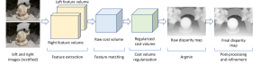
Figure 1: The building blocs of a stereo matching pipeline.

Traditionally, this problem has been solved using a pipeline of four building blocks [11], see Fig. 1: (1) feature extraction, (2) feature matching across images, (3) disparity computation, and (4) disparity refinement and post-processing. The first two blocks construct the cost volume $C$. The third block regularizes the cost volume and then finds, by minimizing Eqn. (1), an initial estimate of the disparity map. The last block refines and post-processes the initial disparity map.

This section focuses on how these individual blocks have been implemented using deep learning-based methods. Table II summarises the state-of-the-art methods.

4.1 Learning feature extraction and matching

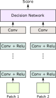
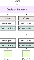
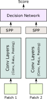
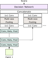
(a) MC-CNN [39, 42].	(b) [37] and [38].	(c) [37].	(d) LW-CNN [48].	(e) FED-D2DRR [49].	(f) [37].

Figure 2: Feature learning architectures.

Early deep learning techniques for stereo matching replace the hand-crafted features (block A of Fig. LABEL:ig:stereo_matching_pipeline) with learned features [37, 38, 39, 42]. They take two patches, one centered at a pixel $x=(i,j)$ on the left image and another one centered at pixel $y=(i,j-d)$ on the right image (with $d\in\{0,\dots,n_{d}\}$), compute their corresponding feature vectors using a CNN, and then match them (block B of Fig. LABEL:ig:stereo_matching_pipeline), to produce a similarity score $C(x,d)$, using either standard similarity metrics such as the $L_{1}$, the $L_{2}$, and the correlation metric, or metrics learned using a top network. The two components can be trained either separately or jointly.

4.1.1 The basic network architecture

The basic network architecture, introduced in [37, 38, 39, 42] and shown in Fig. 2-(a), is composed of two CNN encoding branches, which act as descriptor computation modules. The first branch takes a patch around a pixel $x=(i,j)$ on the left image and outputs a feature vector that characterizes that patch. The second branch takes a patch around the pixel $y=(i,j-d)$, where $d\in[d_{min},d_{max}]$ is a candidate disparity. Zbontar and LeCun [39] and later Zbontar et al. [42] use an encoder composed of four convolutional layers, see Fig. 2-(a). Each layer, except the last one, is followed by a ReLU unit. Zagoruyko and Komodakis [37] and Han et al. [38] use a similar architecture but add:

• max-pooling and subsampling after each layer, except the last one, see Fig. 2-(b). As such, the network is able to account for larger patch sizes and a larger variation in the viewpoint compared to [39, 42].

• a Spatial Pyramid Pooling (SPP) module at the end of each feature extraction branch [37] so that the network can process patches of arbitrary sizes while producing features of a fixed size, see Fig. 2-(c). Its role is to aggregate the features of the last convolutional layer, through spatial pooling, into a feature grid of a fixed size. The module is designed in such a way that the size of the pooling regions varies with the size of the input to ensure that the output feature grid has a fixed size independently of the size of the input patch or image. Thus, the network is able to process patches/images of arbitrary sizes and compute feature vectors of the same dimension without changing its structure or retraining.

The learned features are then fed to a top module, which returns a similarity score. It can be implemented as a standard similarity metric, e.g., the $L_{2}$ distance, the cosine distance, and the (normalized) correlation distance (or inner product) as in the MC-CNN-fast (MC-CNN-fst) architecture of [39, 42]. The main advantage of the correlation over the $L_{2}$ distance is that it can be implemented using a layer of 2D [51] or 1D [22] convolutional operations, called correlation layer. A correlation layer does not require training since the filters are in fact the features computed by the second branch of the network. As such, correlation layers have been extensively used in the literature [39, 41, 42, 22, 44].

Instead of using hand-crafted similarity measures, recent works use a decision network composed of fully-connected (FC) layers [38, 37, 42, 46, 49], which can be implemented as $1\times 1$ convolutions, fully convolutional layers [47], or convolutional layers followed by fully-connected layers. The decision network is trained jointly with the feature extraction module to assess the similarity between two image patches. Han et al. [38] use a top network composed of three fully-connected layers followed by a softmax. Zagoruyko and Komodakis [37] use two linear fully connected layers (each with $512$ hidden units) that are separated by a ReLU activation layer while the MC-CNN-acrt network of Zbontar et al. [42] use up to five fully-connected layers. In all cases, the features computed by the two branches of the feature encoding module are first concatenated and then fed to the top network. Hartmann et al. [47], on the other hand, aggregate the features coming from multiple patches using mean pooling before feeding them to a decision network. The main advantage of aggregation by pooling over concatenation is that the former can handle any arbitrary number of patches without changing the architecture of the network or re-training it. As such, it is suitable for computing multi-patch similarity.

Using a decision network instead of hand-crafted similarity measures enables learning, from data, the appropriate similarity measure instead of imposing one at the outset. It is more accurate than using a correlation layer but is significantly slower.

4.1.2 Network architecture variants

Since its introduction, the baseline architecture has been extended in several ways in order to: (1) improve training using residual networks (ResNet) [46], (2) enlarge the receptive field of the network without losing in resolution or in computation efficiency [48, 49, 52], (3) handling multiscale features [37, 40], (4) reducing the number of forward passes [37, 44], and (5) easing the training procedure by learning similarity without explicitly learning features [37].

4.1.2.1 ConvNet vs. ResNet

While Zbontar et al. [39, 42] and Han et al. [38] use standard convolutional layers in the feature extraction block, Shaked and Wolf [46] add residual blocks with multilevel weighted residual connections to facilitate the training of very deep networks. Its particularity is that the network learns by itself how to adjust the contribution of the added skip connections. It was demonstrated that this architecture outperforms the base network of Zbontar et al. [39].

4.1.2.2 Enlarging the receptive field of the network

The scale of the learned features is defined by (1) the size of the input patches, (2) the receptive field of the network, and (3) the kernel size of the convolutional filters and pooling operations used in each layer. While increasing the kernel sizes allows the capture of more global interactions between the image pixels, it induces a high computational cost. Also, the conventional pooling, as used in [39, 42], reduces resolution and could cause the loss of fine details, which is not suitable for dense correspondence estimation.

To enlarge the receptive field without losing resolution or increasing the computation time, some techniques, e.g.,  [52], use dilated convolutions, i.e., large convolutional filters but with holes and thus they are computationally efficient. Other techniques, e.g.,  [48, 49], use spatial pyramid pooling (SPP) modules placed at different locations in the network, see Fig. 2-(c-e). For instance, Park et al. [48], who introduced FW-CNN for stereo matching, append an SPP module at the end of the decision network, see Fig. 2-(d). As a result, the receptive field can be enlarged. However, for each pixel in the reference image, both the fully-connected layers and the pooling operations need to be computed $n_{d}$ times where $n_{d}$ is the number of disparity levels. To avoid this, Ye et al. [49] place the SPP module at the end of each feature computation branch, see Figs. 2-(c) and (e). In this way, it is only computed once for each patch. Also, Ye et al. [49] employ multiple one-stride poolings, with different window sizes, to different layers and then concatenate their outputs to generate the feature maps, see Fig. 2-(e).

4.1.2.3 Learning multiscale features

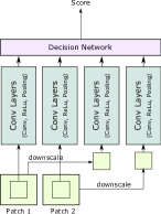
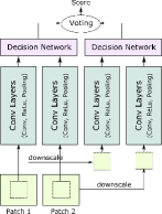
(a) Center-surround [37]	(b) Voting-based [40].

Figure 3: Multiscale feature learning architectures.

The methods described so far can be extended to learn features at multiple scales by using multi-stream networks, one stream per patch size [37, 40], see Fig. 3. Zagoruyko and Komodakis [37] propose a two-stream network, which is essentially a network composed of two siamese networks combined at the output by a top network, see Fig. 3-(a). The first siamese network, called central high-resolution stream, receives as input two $32\times 32$ patches centered around the pixel of interest. The second network, called surround low-resolution stream, receives as input two $64\times 64$ patches but down-sampled to $32\times 32$. The output of the two streams are then concatenated and fed to a top decision network, which returns a matching score. Chen et al. [40] use a similar approach but instead of aggregating the features computed by the two streams prior to feeding them to the top decision network, it appends a top network on each stream to produce a matching score. The two scores are then aggregated by voting, see Fig. 3-(b).

The main advantage of the multi-stream architecture is that it can compute features at multiple scales in a single forward pass. It, however, requires one stream per scale, which is not practical if more than two scales are needed.

4.1.2.4 Reducing the number of forward passes

Using the approaches described so far, inferring the raw cost volume from a pair of stereo images is performed using a moving window-like approach, which would require multiple forward passes, $n_{d}$ forward passes per pixel where $n_{d}$ is the number of disparity levels. However, since correlations are highly parallelizable, the number of forward passes can be significantly reduced. For instance, Luo et al. [44] reduce the number of forward passes to one pass per pixel by using a siamese network, whose first branch takes a patch around a pixel while the second branch takes a larger patch that expands over all possible disparities. The output is a single 64D representation for the left branch, and $n_{d}\times 64$ for the right branch. A correlation layer then computes a vector of length $n_{d}$, where its $0pt-$th element is the cost of matching the pixel $x$ on the left image with the pixel $x-0pt$ on the rectified right image.

Zagoruyko and Komodakis [37] showed that the outputs of the two feature extraction sub-networks need to be computed only once per pixel, and do not need to be recomputed for every disparity under consideration. This can be done in a single forward pass, for the entire image, by propagating full-resolution images instead of small patches. Also, the output of the top network composed of fully-connected layers in the accurate architecture (i.e., MC-CNN-Accr) can be computed in a single forward pass by replacing the fully-connected layers with convolutional layers of $1\times 1$ kernels. However, it still requires one forward pass for each disparity under consideration.

4.1.2.5 Learning similarity without feature learning

Joint training of feature extraction and similarity computation networks unifies the feature learning and the metric learning steps. Zagoruyko and Komodakis [37] propose another architecture that does not have a direct notion of features, see Fig. 2-(f). In this architecture, the left and right patches are packed together and fed jointly into a two-channel network composed of convolution and ReLU layers followed by a set of fully connected layers. Instead of computing features, the network directly outputs the similarity between the input pair of patches. Zagoruyko and Komodakis [37] showed that this architecture is easy to train. However, it is expensive at runtime since the whole network needs to be run $n_{d}$ times per pixel.

4.1.3 Training procedures

The networks described in this section are composed of a feature extraction block and a feature matching block. Since the goal is to learn how to match patches, these two modules are jointly trained either in a supervised (Section 4.1.3.1) or in a weakly supervised manner (Section 4.1.3.2).

4.1.3.1 Supervised training

Existing methods for supervised training use a training set composed of positive and negative examples. Each positive (respectively negative) example is a pair composed of a reference patch and its matching patch (respectively a non-matching one) from another image. Training either takes one example at a time, positive or negative, and adapts the similarity [40, 41, 38, 37], or takes at each step both a positive and a negative example, and maximizes the difference between the similarities, hence aiming at making the two patches from the positive pair more similar than the two patches from the negative pair [43, 45, 39]. This latter scheme is known as Triplet Contrastive learning.

Zbontar et al. [39, 42] use the ground-truth disparities of the KITTI2012 [15] or Middlebury [20] datasets. For each known disparity, the method extracts one negative pair and one positive pair as training examples. As such, the method is able to extract more than $25$ million training samples from KITTI2012 [15] and more than $38$ million from the Middlebury dataset [20]. This method has been also used by Chen et al. [40], Zagoruyku and Komodakis [37], and Han et al. [38]. The amount of training data can be further augmented by using data augmentation techniques, e.g., flipping patches and rotating them in various directions.

Although the supervised learning works very well, the complexity of the neural network models requires very large labeled training sets, which are hard or costly to collect for real applications (e.g., consider the stereo reconstruction of the Mars landscape). Even when such large sets are available, the ground truth is usually produced from depth sensors and often contains noise that reduces the effectiveness of the supervised learning [53]. This can be mitigated by augmenting the training set with random perturbations [39] or synthetic data [54, 22]. However, synthesis procedures are hand-crafted and do not account for the regularities specific to the stereo system and target scene at hand.

Loss functions. Supervised stereo matching networks are trained to minimize a matching loss, which is a function that measures the discrepancy between the ground-truth and the predicted matching scores for each training sample. It can be defined using (1) the $L_{1}$ distance [42, 40, 46], (2) the hinge loss [42, 46], or (3) the cross-entropy loss [44].

4.1.3.2 Weakly supervised learning

Weakly supervised techniques exploit one or more stereo constraints to reduce the amount of manual labelling. Tulyakov et al. [50] consider Multi-Instance Learning (MIL) in conjunction with stereo constraints and coarse information about the scene to train stereo matching networks with datasets for which ground truth is not available. Unlike supervised techniques, which require pairs of matching and non-matching patches, the training set is composed of $N$ triplets. Each triplet is composed of: (1) $W$ reference patches extracted on a horizontal line of the reference image, (2) $W$ positive patches extracted from the corresponding horizontal line on the right image, and (3) $W$ negative patches, i.e., patches that do not match the reference patches, extracted from another horizontal line on the right image. As such, the training set can automatically be constructed from stereo pairs without manual labelling.

The method is then trained by exploiting five constraints: the epipolar constraint, the disparity range constraint, the uniqueness constraint, the continuity (smoothness) constraint, and the ordering constraint. They then define three losses that use different subsets of these constraints, namely:

• The Multi Instance Learning (MIL) loss, which uses the epipolar and the disparity range constraints. From these two constraints, we know that every non-occluded reference patch has a matching positive patch in a known index interval, but does not have a matching negative patch. Therefore, for every reference patch, the similarity of the best reference-positive match should be greater than the similarity of the best reference-negative match.

• The constractive loss, which adds to the MIL method the uniqueness constraint. It tells us that the matching positive patch is unique. Thus, for every patch, the similarity of the best match should be greater than the similarity of the second best match.

• The constractive-DP uses all the constraints but finds the best match using dynamic programming.

The method has been applied to train a deep siamese neural-network that takes two patches as an input and predicts a similarity measure. Benchmarking on standard datasets shows that the performance is as good or better than the published results on MC-CNN-fst [39], which uses the same network architecture but trained using fully labeled data.

4.2 Regularization and disparity estimation

Once the raw cost volume is estimated, one can estimate the disparity by dropping the regularization term of Eqn. (1), or equivalently block C of Fig. 1, and taking the argmin, the softargmin, or the subpixel MAP approximation (block D of Fig. 1). However, the raw cost volume computed from image features could be noise-contaminated, e.g., due to the existence of non-Lambertian surfaces, object occlusions, or repetitive patterns. Thus, the estimated depth maps can be noisy. As such, some methods overcome this problem by using traditional MRF-based stereo framework for cost volume regularization [40, 39, 44]. In these methods, the initial cost volume $C$ is fed to a global [11] or a semi-global [55] matcher to compute the disparity map. Semi-global matching provides a good tradeoff between accuracy and computation requirements. In this method, the smoothness term of Eqn. (1) is defined as:

$$\small{E_{s}(0pt_{x},0pt_{y})=\alpha_{1}\delta(|0pt_{xy}=1)+\alpha_{2}\delta(|0pt_{xy}>1),}$$ (2)

where $0pt_{xy}=0pt_{x}-0pt_{y}$, $\alpha_{1}$ and $\alpha_{2}$ are positive weights chosen such that $\alpha_{2}>\alpha_{1}$, and $\delta$ is the Kronecker delta function, which gives $1$ when the condition in the bracket is satisfied, otherwise $0$. To solve this optimisation problem, the SGM energy is broken down into multiple energies $E_{s}$, each one defined along a path $s$. The energies are minimised independently and then aggregated. The disparity at $x$ is computed using the winner-takes-all strategy of the aggregated costs of all directions:

$$d_{x}=\arg\min_{d}\sum_{s}E_{s}(x,d).$$ (3)

This method requires setting the two parameters $\alpha_{1}$ and $\alpha_{2}$ of Eqn. (2). Instead of manually setting them, Seki et al. [56] proposed SGM-Net, a neural network trained to provide these parameters at each image pixel. They obtained better penalties than hand-tuned methods as in [39].

The SGM method, which uses an aggregated scheme to combine costs from multiple 1D scanline optimizations, suffers from two major issues: (1) streaking artifacts caused by the scanline optimization approach, at the core of this algorithm, may lead to inaccurate results, and (2) the high memory footprint that may become prohibitive with high resolution images or devices with constrained resources. As such Schonberger et al. [57] reformulate the fusion step as the task of selecting the best amongst all the scanline optimization proposals at each pixel in the image. They solve this task using a per-pixel random forest classifier.

Poggi et al. [58] learn a weighted aggregation where the weight of each 1D scanline optimisation is defined using a confidence map computed using either traditional techniques [59] or deep neural networks, see Section 5.5.

5 End-to-end depth from stereo

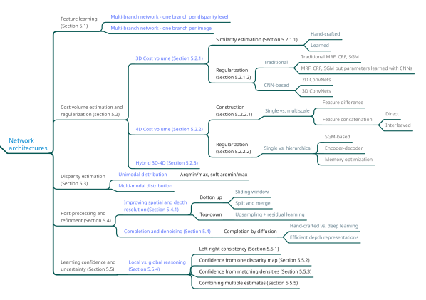
Figure 4: Taxonomy of the network architectures for stereo-based disparity estimation using end-to-end deep learning.

Recent works solve the stereo matching problem using a pipeline that is trained end-to-end. Two main classes of methods have been proposed. Early methods, e.g., FlowNetSimple [51] and DispNetS [22], use a single encoder-decoder, which stacks together the left and right images into a 6D volume, and regresses the disparity map. These methods, which do not require an explicit feature matching module, are fast at runtime. They, however, require a large amount of training data, which is hard to obtain. Methods in the second class mimic the traditional stereo matching pipeline by breaking the problem into stages, each stage is composed of differentiable blocks and thus allowing end-to-end training. Below, we review in details these techniques. Fig. 4 provides a taxonomy of the state-of-the-art, while Table III compares $28$ key methods based on this taxonomy.

5.1 Feature learning

Feature learning networks follow the same architectures as the ones described in Figs. 2 and 3. However, instead of processing individual patches, the entire images are processed in a single forward pass producing feature maps of the same or lower resolution as the input images. Two strategies have been used to enable matching features across the images:

(1) Multi-branch networks composed of $n$ branches where $n$ is the number of input images. Each branch produces a feature map that characterizes its input image [22, 60, 61, 62, 63, 64, 65]. These techniques assume that the input images have been rectified so that the search for correspodnences is restricted to be along the horizontal scanlines.

(2) Multi-branch networks composed of $n_{d}$ branches where $n_{d}$ is the number of disparity levels. The $d$-th branch, $1\leq d\leq n_{d}$, processes a stack of two images, as in Fig. 2-(f); the first image is the reference image. The second one is the right image but re-projected to the $d$-th depth plane [66]. Each branch produces a similarity feature map that characterizes the similarity between the reference image and the right image re-projected onto a given depth plane. While these techniques do not rectify the images, they assume that the intrinsic and extrinsic camera parameters are known. Also, the number of disparity levels cannot be varied without updating the network architecture and retraining it.

In both methods, the feature extraction module uses either fully convolutional (ConvNet) networks such as VGG, or residual networks such as ResNets [67]. The latter facilitates the training of very deep networks [68]. They can also capture and incorporate more global context in the unary features by using either dilated convolutions (Section 4.1.2.2) or multi-scale approaches. For instance, the PSM-Net of Chang and Chen [64] append a Spatial Pyramid Pooling (SPP) module in order to extract and aggregate features at multiple scales. Nie et al. [65] extended PSM-Net using a multi-level context aggregation pattern termed Multi-Level Context Ultra-Aggregation (MLCUA). It encapsulates all convolutional features into a more discriminative representation by intra and inter-level features combination. It combines the features at the shallowest, smallest scale with features at deeper, larger scales using just shallow skip connections. This results in an improved performance, compared to PSM-Net [64], without significantly increasing the number of parameters in the network.

TABLE III: Taxonomy and comparison of $28$ end-to-end deep learning-based disparity estimation techniques. ”FCN”: Fully-Connected Network, ”SPN”: Spatial Propagation Network. ”LRCR”: Left-Right Comparative Recurrent model, ”MCUA”: Multi-Level Context Ultra-Aggregation for Stereo Matching. ”DLA”: Deep layer aggregation [69], ”VPP”: Volumetric Pyramid Pooling. The performance is measured on KITTI2015 test dataset.

Method

Year

Feature computation

Cost volume

Disparity

Refinement/post processing

Supervision

Performance

Architecture

Dimension

Type

Construction

Regularization

Spatial/depth resolution

Completion/denoising

D1-all/est

D1-all/fg

FlowNetCorr [51]

2015

ConvNet

Single scale

3D

Correlation

2D ConvNet

Up-convolutions

Ad-hoc, variational

Supervised

$-$

$-$

DispNetC [22]

2016

ConvNet

Single scale

3D

Correlation

2D ConvNet

$-$

$-$

$-$

Supervised

$4.34$

$4.32$

Zhong et al. [70]

2017

ConvNet

Single scale

4D

Interleaved

3D Conv,

Soft argmin

Self-improvement at runtime

Self-supervised

$3.57$

$7.12$

with skip conn.

feature concat.

encoder-decoder

Kendall et al. [61]

2017

ConvNet

Single scale

4D

Feature concat.

3D Conv, encoder-

Soft argmax

$-$

$-$

Supervised

$2.87$

$6.16$

with skip conn.

decoder, hierarchical

Pang et al. [62]

2017

ConvNet

Single scale

3D

Correlation

2D ConvNet

Upsampling$+$ residual learning

Supervised

$2.67$

$3.59$

Knobelreiter et al. [71]

2017

ConvNet

Single scale

3D

Correlation

Hybrid CNN-CRF

No post-processing

Supervised

Chang et al. [64]

2018

SPP

Multiscale

4D

Feature concat.

3D Conv, Stacked encoder-decoders

Soft argmin

Progressive refinement

Supervised

$2.32$

$4.62$

Khamis et al. [72]

2018

ResNet

Single scale

3D

$L_{2}$

3D ConvNet

Soft argmin

Hierarchical, Upsamling$+$residual learning

Supervised

$4.83$

$7.45$

Liang et al. [63]

2018

ConvNet

Multiscale

3D

Correlation

2D ConvNet

Encoder-decoder

Iterative upsampling$+$residual learning

Supervised

$2.67$

$3.59$

Yang et al. [68]

2018

Shallow

Single scale

3D

Correlation, Left features, segmentation mask

Regression with

$-$

$-$

Self-supervised

$2.25$

$4.07$

ResNet

Encoder-decoder

Zhang et al. [73]

2018

ConvNet

Single scale

3D

Hand-crafted

NA

Soft argmin

Upsampling$+$residual learning

Self-supervised

$-$

$-$

Jie et al. [74]

2018

Constant highway net

Single scale

3D

FCN

$-$

RNN-based LRCR

$-$

$-$

Supervised

$3.03$

$5.42$

Ilg et al. [75]

2018

ConvNet

Single scale

3D

Correlation

Encoder-decoder, joint disparity and occlusion

Cascade of encoder-decoders, residual learning

Supervised

$2.19$

$-$

Song et al. [76]

2018

SHallow ConvNet

Single scale

3D

Correlation

Edge-guided, Context Pyramid,

Residual pyramid

$-$

$-$

Supervised

$2.59$

$4.18$

Encoder

Yu et al. [77]

2018

ResNet

Single scale

3D

Feature concatenation

3D Conv $+$ SGM

Soft argmin

$-$

$-$

Supervised

$2.79$

$5.46$

Encoder-decoder

Tulyakov et al. [78]

2018

$-$

Single scale

4D

Compressed

3D Conv

Multimodal -

$-$

$-$

Supervised

$2.58$

$4.05$

matching features

Sub-pixel MAP

EMCUA et al. [65]

2019

SPP

Multiscale

4D

Feature concat.

3D Conv, MCUA scheme

Arg softmin

$-$

$-$

Supervised

$2.09$

$4.27$

Yang et al. [32]

2019

SPP

Multiscale

Pyramidal 4D

Feature difference

Conv3D blocks $+$ Volume Pyramid Pooling

Arg softmax

Spatial & depth res. by cost volume upsampling

Supervised

$2.14$

$3.85$

Wu et al. [79]

2019

ResNet50, SPP

Multiscale

Pyramidal 4D

Feature concat.

Encoder-decoder

3D Conv, soft argmin

$-$

$-$

Supervised

$2.11$

$3.89$

$+$ Feature fusion

Disparity & boundary loss

Yin et al. [80]

2019

DLA net

Multiscale

3D

Correlation

Density decoder

Outputs discrete

$-$

$-$

Supervised

2.02

$3.63$

matching distribution

Chabra et al. [81]

2019

ConvNet $+$

Multiscale

3D

$L_{1}$

Dilated 3D ConvNet

Soft argmax

Upsampling$+$residual learning

Supervised

$2.26$

$4.95$

Vortex pooling [82]

Duggal et al. [83]

2019

ResNet, SPP

Multiscale

3D, sparse

Correlation, Adaptive

Encoder-decoder

Soft argmax

Encoder

$-$

Supervised

$2.35$

3.43

pruning with PatchMatch

Tonioni et al. [84]

2019

ConvNet

Multiscale

3D

Correlation

Encoder

Recrusively upsampling $+$ residual learning

Online self-adaptive

$4.66$

$-$

Yang et al. [32]

2019

ConvNet, SPP

Multiscale

Pyramid, 4D

Concatenation

Decoder, Residual blocs,

Conv3D block

$-$

$-$

Supervised

$2.14$

$3.85$

VPP

Zhang et al. [85]

2019

Stacked hourglass

Single scale

4D

Concatenation

Semi-global aggregation layers,

Soft argmax

$-$

$-$

Supervised

$2.03$

$3.91$

Local-guided aggregation layers

Guo et al. [86]

2019

SPP

Multiscale

Hybrid 3D-4D

Group-wise correlation

Stacked hourglass nets

Soft argmin

$-$

$-$

Supervised

$2.11$

$3.93$

Chen et al. [87]

2019

Single-modal weighted avg

Supervised

$2.14$

$4.33$

Wang et al. [88]

2019

ConvNet

Multiresolution maps

3D

$L_{1}$

Progressive refinement

Soft argmin

Usampling,

Spatial propagation

Supervised

$-$

$-$

(3D Conv)

residual learning

network

5.2 Cost volume construction

Once the features have been computed, the next step is to compute the matching scores, which will be fed, in the form of a cost volume, to a top network for regularization and disparity estimation. The cost volume can be three dimensional (3D) where the third dimension is the disparity level (Section 5.2.1), four dimensional (4D) where the third dimension is the feature dimension and the fourth one is the disparity level (Section 5.2.2), or hybrid to benefit from the properties of the 3D and 4D cost volumes (Section 5.2.3). In general, the cost volume is constructed at a lower resolution, e.g., at $\nicefrac{{1}}{{8}}$-th, than the input [72, 73]. It is then either subsequently upscaled and refined, or used as is to estimate a low resolution disparity map, which is then upscaled and refined using a refinement module.

5.2.1 3D cost volumes

5.2.1.1 Construction

A 3D cost volume can be simply built by taking the $L_{1}$, $L_{2}$, or correlation distance between the features of the left image and those of the right image that are within a pre-defined disparity range, see [22, 73, 74, 72, 80, 81, 83], and the FlowNetCorr of [51]. The advantage of correlation-based dissimilarities is that they can be implemented using a convolutional layer that does not require training (its filters are the features computed by the second branch of the network). Flow estimation networks such as FlowNetCorr [51] use 2D correlations. Disparity estimation networks, such as [22, 68], iResNet [63], DispNet3 [75], EdgeStereo [76], HD³ [80], and [84, 83], use 1D correlations.

5.2.1.2 Regularization of 3D cost volumes

Once a cost volume is computed, an initial disparity map can be estimated using the argmin, the softargmin, or the subpixel MAP approximation over the depth dimension of the cost volume, see for example [73] and Fig. 5-(a). This is equivalent to dropping the regularization term of Eqn. (1). In general, however, the raw cost volume is noise-contaminated (e.g., due to the existence of non-Lambertian surfaces, object occlusions, and repetitive patterns). The goal of the regularization module is to leverage context along the spatial and/or disparity dimensions to refine the cost volume before estimating the initial disparity map.

(1) Regularization using traditional methods. Early papers use traditional techniques, e.g., Markov Random Fields (MRF), Conditional Random Fields (CRF), and Semi-Global Matching (SGM), to regularize the cost volume by explicitly incorporating spatial constraints, e.g., smoothness, of the depth maps. Recent papers showed that deep learning networks can be used to fine-tune the parameters of these methods. For example, Knöbelreiter et al. [71] proposed a hybrid CNN-CRF. The CNN computes the matching term of Eqn. (1), which becomes the unary term of a CRF module. The pairwise term of the CRF is parameterized by edge weights computed using another CNN. The end-to-end trained CNN-CRF pipeline could achieve a competitive performance using much fewer parameters (thus a better utilization of the training data) than the earlier methods.

Zheng et al. [89] provide a way to model CRFs as recurrent neural networks (RNN) for segmentation tasks so that the entire pipeline can be trained end-to-end. Unlike segmentation, in depth estimation, the number of depth samples, whose counterparts are the semantic labels in segmentation tasks, is expected to vary for different scenarios. As such, Xue et al. [90] re-designed the RNN-formed CRF module so that the model parameters are independent of the number of depth samples. Paschalidou et al. [91] formulate the inference in a MRF as a differentiable function, hence allowing end-to-end training using back propagation. Note that Zheng et al. [89] and Paschalidou et al. [91] focus on multi-view stereo (Section 6). Their approaches, however, are generic and can be used to regularize 3D cost volumes obtained using pairwise stereo networks.

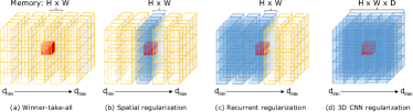
Figure 5: Cost volume regularization schemes [92]: (a) does not consider context, (b) captures context along the spatial dimensions using 2D convolutions, (c) captures context along the spatial and disparity dimensions by recurrent regularization using 2D convolutions, and (d) captures context in all dimensions by using 3D convolutions.

(2) Regularization using 2D convolutions (2DConvNet), Figs. 5-(b) and (c). Another approach is to process the 3D cost volume using a series of 2D convolutional layers producing another 3D cost volume [22, 51, 62, 63]. 2D convolutions are computationally efficient. However, they only capture and aggregate context along the spatial dimensions, see Fig. 5-(b), and ignore context along the disparity dimension. Yao et al. [92] sequentially regularize the 2D cost maps along the depth direction via a Gated Recurrent Unit (GRU), see Fig. 5-(c). This reduces drastically the memory consumption, e.g., from $15.4$GB in [93] to around $5$GB, making high-resolution reconstruction feasible, while capturing context along both the spatial and the disparity dimensions.

(3) Regularization using 3D convolutions (3DConvNet), Fig. 5-(d). Khamis et al. [72] use the $L_{2}$ distance to compute an initial 3D cost volume and 3D convolutions to regularize it across both the spatial and disparity dimensions, see Fig. 5-(d). Due to its memory requirements, the approach first estimates a low-resolution disparity map, which is then progressively improved using residual learning. Zhang et al. [73] follow the same approach but the refinement block starts with separate convolution layers running on the upsampled disparity and input image respectively, and merge the features later to produce the residual. Chabra et al. [81] observe that the cost volume regularization step is the one that uses most of the computational resources. They then propose a regularization module that uses 3D dilated convolutions in the width, height, and disparity dimesions, to reduce the computation time while capturing a wider context.

5.2.2 4D cost volumes

5.2.2.1 Construction

4D cost volumes to preserve the dimension of the features [70, 61, 64, 65, 32, 79]. The rational behind 4D cost volumes is to let the top network learn the appropriate similarity measure for comparing the features instead of using hand-crafted ones as in Section 5.2.1.

4D cost volumes can be constructed by feature differences across a pre-defined disparity range [32], which results in cost volume of size $0pt\times 0pt\times 2n_{d}\times c$, or by concatenating the features computed by the different branches of the network [61, 70, 64, 65, 79]. Using this method, Kendall et al. [61] build a 4D volume of size $0pt\times 0pt\times(n_{d}+1)\times c$ ($c$ here is the dimension of the features). Zhong et al. [70] follow the same approach but concatenate the features in an interleaved manner. That is, if $\textbf{f}_{L}$ is the feature map of the left image and $\textbf{f}_{R}$ the feature map of the right image, then the final feature volume is assembled in such a way that its $2i-$th slice holds the left feature map while the $(2i+1)-$th slice holds the right feature map but at disparity $d=i$. This results in a 4D cost volume that is twice larger than the cost volume of Kendall et al. [61]. To capture multi-scale context in the cost volume, Chang and Chen [64] generate for each input image a pyramid of features, upsamples them to the same dimension, and then builds a single 4D cost volume by concatenation. Wu et al. [79] build from the multiscale features (four scales) multiscale 4D cost volumes.

4D cost volumes carry richer information compared to 3D cost volumes. Note, however, that volumes obtained by concatenation contain no information about the feature similarities, so more parameters are required in the subsequent modules to learn the similarity function.

5.2.2.2 Regularization of 4D cost volumes

4D cost volumes are regularized with 3D convolutions, which exploit the correlation in height, width and disparity dimensions, to produce a 3D cost volume. Kendall et al. [61] use a U-net encoder-decoder with 3D convolutions and skip connections. Zhong et al. [70] use a similar approach but add residual connections from the contracting to the expanding parts of the regularization network. To take into account a large context without a significant additional computational burden, Kendall et al. [61] regularize the cost volume hierarchically, with four levels of subsampling, allowing to explicitly leverage context with a wide field of view. Muliscale 4D cost volumes [79] are aggregated into a single 3D cost volume using a 3D multi-cost aggregation module, which operates in a pairwise manner starting with the smallest volume. Each volume is processed with an encoder-decoder, upsampled to the next resolution in the pyramid, and then fused using a 3D feature fusion module.

Also, semi-global matching (SGM) techniques have been used to regularize the 4D cost volume where their parameters are estimated using convolutional networks. In particular, Yu et al. [77] process the initial 4D cost volume with an encoder-decoder composed of 3D convolutions and upconvolutions, and produces another 3D cost volume. The subsequent aggregation step is performed using an end-to-end two-stream network: the first stream generates three cost aggregation proposals $C_{i}$, one along each of the tree dimensions, i.e., the height, width, and disparity. The second stream is a guidance stream used to select the best proposals. It uses 2D convolutions to produce three guidance (confidence) maps $W_{i}$. The final 3D cost volume is produced as a weighted sum of the three proposals, i.e., $\max_{i}(C_{i}*W_{i})$.

3D convolutions are expensive in terms of memory requirements and computation time. As such, subsequent works that followed the seminal work of Kendall et al. [61] focused on (1) reducing the number of 3D convolutional layers [85], (2) progressively refining the cost volume and the disparity map [64, 88], and (3) compressing the 4D cost volume [78]. Below, we discuss these approaches.

(1) Reducing the number of 3D convolutional layers. Zhang et al. [85] introduced GANet, which replaces a large number of the 3D convolutional layers in the regularization block with (1) two 3D convolutional layers, (2) a semi-global aggregation layer (SGA), and (3) a local guided aggregation layer (LGA). SGA is a differentiable approximation of the semi-global matching (SGM). Unlike SGM, in SGA the user-defined parameters are learnable. Moreover, they are added as penalty coefficients/weights of the matching cost terms. Thus, they are adaptive and more flexible at different locations for different situations. The LGA layer, on the other hand, is appended at the end and aims to refine the thin structures and object edges. The SGA and LGA layers, which are used to replace the costly 3D convolutions, capture local and whole-image cost dependencies. They significantly improve the accuracy of the disparity estimation in challenging regions such as occlusions, large textureless/reflective regions, and thin structures.

(2) Progressive approaches. Some techniques avoid directly regularizing high resolution 4D cost volumes using the expensive 3D convolutions. Instead, they operate in a progressive manner. For instance, Chang and Chen [64] introduced PSM-Net, which first estimates a low resolution 4D cost volume, and then regularizes it using stacked hourglass 3D encoder-decoder blocks. Each block returns a 3D cost volume, which is then upsampled and used to regress a high resolution disparity map using additional 3D convolutional layers followed by a softmax operator. As such, the stacked hourglass blocks can be seen as refinement modules.

Wang et al. [88] use a three-stage disparity estimation network, called AnyNet, which builds cost volumes in a coarse-to-fine manner. The first stage takes as input low resolution feature maps, builds a low resolution 4D cost volume and then uses 3D convolutions to estimate a low resolution disparity map by searching on a small disparity range. The prediction in the previous level is then upsampled and used to warp the input feature at the higher scale, with the same disparity estimation network used to estimate disparity residuals. The advantage is two-fold; first, at higher resolutions, the network only learns to predict residuals, which reduces the computation cost. Second, the approach is progressive and one can select to return the intermediate disparities, trading accuracy for speed.

(3) 4D cost volume compression. Tulyakov et al. [78] reduce the memory usage, without having to sacrify accuracy, by compressing the features into compact matching signatures. As such, the memory footprint is significantly reduced. More importantly, it allows the network to handle an arbitrary number of multiview images and to vary the number of inputs at runtime without having to re-train the network.

5.2.3 Hybrid 3D-4D cost volumes

The correlation layer provides an efficient way to measure feature similarities, but it loses much information because it produces only a single-channel map for each disparity level. On the other hand, 4D cost volumes obtained by feature concatenation carry more information but are resource-demanding. They also require more parameters in the subsequent aggregation network to learn the similarity function. To benefit from both, Guo et al. [86] propose a hybrid approach, which constructs two cost volumes; one by feature concatenation but compressed into $12$ channels using two convolutions. The second one is built by dividing the high-dimension feature maps into $N_{g}$ groups along the feature channel, computing correlations within each group at all disparity levels, and finally concatenating the correlation maps forming another 4D volume. The two volumes are then combined together and passed to a 3D regularization module composed of four 3D convolution layers followed by three stacked 3D hourglass networks. This approach results in a significant reduction of parameters compared to 4D cost volumes built by only feature concatenation, without losing too much information like full correlations.

5.3 Disparity computation

The simplest way to estimate the disparity map from the regularized cost volume $C$ is by using the pixel-wise argmin, i.e., $0pt_{x}=\arg\min_{0pt}C(x,0pt)$ (or equivalently $\arg\max$ if the volume $C$ encodes the likelihood). However, the agrmin/argmax operator is unable to produce sub-pixel accuracy and cannot be trained with back-propagation due to its non-differentiability. Another approach is the differentiable soft argmin/max over disparity [66, 61, 73, 72]:

$$d^{*}=\frac{1}{\sum_{j=0}^{n_{d}}e^{-C(x,j)}}\sum_{d=0}^{n_{d}}d\times e^{-C(x,d)}.$$ (4)

The soft argmin operator approximates the sub-pixel MAP solution when the distribution is unimodal and symmetric [78]. When this assumption is not fulfilled, the softargmin blends the modes and may produce a solution that is far from all the modes and may result in over smoothing. Chen et al. [87] observe that this is particularly the case at boundary pixels where the estimated disparities follow multimodal distributions. To address these issues, Chen et al. [87] only apply a weighted average operation on a window centered around the modal with the maximum probability, instead of using a full-band weighted average on the entire disparity range.

Tulyakov et al. [78] introduced the sub-pixel MAP approximation, which computes a weighted mean around the disparity with the maximum posterior probability as:

$$d^{*}=\sum_{d:|\hat{d}-d|\leq\delta}d\cdot\sigma(C(x,d)),$$ (5)

where $\delta$ is a meta parameter set to $4$ in [78], $\sigma(C(x,d))$ is the probability of the pixel $x$ having a disparity $d$, and $\displaystyle\hat{d}=\arg\max_{d}C(x,d)$. The sub-pixel MAP is only used for inference. Tulyakov et al. [78] also showed that, unlike the softargmin/max, this approach allows changing the disparity range at runtime without re-training the network.

5.4 Variants

The pipeline described so far infers disparity maps that can be of low-resolution (along the width, height, and disparity dimensions), incomplete, noisy, missing fine details, and suffering from over-smoothing especially at object boundaries. As such, many variants have been introduced to (1) improve their resolution (Section 5.4.1), (2) improve the processing time, especially at runtime (Section 5.4.3), and (3) perform disparity completion and denoising (Section 5.4.2).

5.4.1 Learning to infer high resolution disparity maps

Directly regressing high-resolution depth maps that contain fine details, e.g., by adding further upconvolutional layers to upscale the cost volume, would require a large number of parameters and thus are computationally expensive and difficult to train. As such, state-of-the-art methods struggle to process high resolution imagery because of memory constraints or speed limitations. This has been addressed by using either bottom-up or top-down techniques.

Bottom-up techniques operate in a sliding window-like approach. They take small patches and estimate the refined disparity either for the entire patch or for the pixel at the center of the patch. Lee et al. [94] follow a split-and-merge approach. The input image is split into regions, and a depth is estimated for each region. The estimates are then merged using a fusion network, which operates in the Fourier domain so that depth maps with different cropping ratios can be handled. While both sliding window and split-and-merge approaches reduce memory requirements, they require multiple forward passes, and thus are not suitable for realtime applications. Also, these methods do not capture the global context, which can limit their performance.

Top-down techniques, on the other hand, operate on the disparity map estimates in a hierarchical manner. They first estimate a low-resolution disparity map and then upsample them to the desired resolution, e.g., using bilinear upsampling, and further process them using residual learning to recover small details and thin structures [72, 73, 81]. This process can also be run progressively by cascading many of such refinement blocks, each block refines the estimate of the previous block [62, 72]. Unlike upsampling cost volumes, refining disparity maps is computationally efficient since it only requires 2D convolutions. Existing methods mainly differ in the type of additional information that is appended to the upsampled disparity map for refinement. For instance:

• Khamis et al. [72] concatenate the upsampled disparity map with the original reference image.

• Liang et al. [63] append to the initial disparity map the cost volume and the reconstruction error, defined as the difference between the left image and the right image but warped to the left image using the estimated disparity map.

• Chabra et al. [81] take the left image and the reconstruction error on one side, and the left disparity and the geometric error map, defined as the difference between the estimated left disparity and right disparity but warped onto the left view. These are independently filtered using one layer of convolutions followed by batch normalization. The results of the two streams are concatenated and then further processed using a series of convolutional layers to produce the refined disparity map.

These methods improve the spatial resolution but not the disparity resolution. To refine both the spatial and depth resolution, while operating on high resolution images, Yang et al. [32] propose to search for correspondences incrementally over a coarse-to-fine hierarchy. The approach constructs a pyramid of four 4D cost volumes, each with increasing spatial and depth resolutions. Each volume is filtered by six 3D convolution blocks, and further processed with a Volumetric Pyramid Pooling block, an extension of Spatial Pyramid Pooling to feature volumes, to generate features that capture sufficient global context for high resolution inputs. The output is then either (1) processed with another conv3D block to generate a 3D cost volume from which disparity can be directly regressed. This allows to report on-demand disparities computed from the current scale, or (2) tri-linearly-upsampled to a higher spatial and disparity resolution so that it can be fused with the next 4D volume in the pyramid. To minimise memory requirements, the approach uses striding along the disparity dimensions in the last and second last volumes of the pyramid. The network is trained end-to-end using a multi-scale loss. This hierarchical design also allows for anytime on-demand reports of disparity by capping intermediate coarse results, allowing accurate predictions for near-range structures with low latency (30ms).

This approach shares some similarities with the approach of Kendall et al. [61], which constructs hierarchical 4D feature volumes and processes them from coarse to fine using 3D convolutions. Kendall et al.’s approach [61], however, has been used to leverage context with a wide field of view while Yang et al. [32] apply coarse-to-fine principles for high-resolution inputs and anytime, on-demand processing.

5.4.2 Learning for completion and denoising

Raw disparities can be noisy and incomplete, especially near object boundaries where depth smearing between objects remains a challenge. Several techniques have been developed for denoising and completion. Some of them are ad-hoc, i.e., post-process the noisy and uncomplete initial estimates to generate clean and complete depth maps. Other methods addressed the issue of the lack of training data for completion and denoising. Others proposed novel depth representations that are more suitable for this task, especially for solving the depth smearing between objects.

Ad-hoc methods process the initially estimated disparities a using variational approaches [51, 95], Fully-Connected CRFs (DenseCRF) [27, 96], hierarchical CRFs [2], and diffusion processes [40] guided by confidence maps [97]. They encourage pixels that are spatially close and with similar colors to have closer disparity predictions. They have been also explored by Liu et al. [5]. However, unlike Li et al. [2], Liu et al. [5] used a CNN to minimize the CRF energy. Convolutional Spatial Propagation Networks (CSPN) [98, 99], which implement an anisotropic diffusion process, are particularly suitable for depth completion since they predict the diffusion tensor using a deep CNN. This is then applied to the initial map to obtain the refined one.

One of the main challenges of deep learning-based depth completion and denoising is the lack of labelled training data, i.e., pairs of noisy, incomplete depth maps and their corresponding clean depth maps. To address this issue, Jeon and Lee [29] propose a pairwise depth image dataset generation method using dense 3D surface reconstruction with a filtering method to remove low quality pairs. They also present a multi-scale Laplacian pyramid based neural network and structure preserving loss functions to progressively reduce the noise and holes from coarse to fine scales. The approach first predicts the clean complete depth image at the coarsest scale, which has a quarter of the original resolution. The predicted depth map is then progressively upsampled through the pyramid to predict the half and original-sized image. At the coarse level, the approach captures global context while at finer scales it captures local information. In addition, the features extracted during the downsampling are passed to the upsampling pyramid with skip connections to prevent the loss of the original details in the input depth image during the upsampling.

Instead of operating on the network architecture, the loss function, or the training datasets, Imran et al. [100] propose a new representation for depth called Depth Coefficients (DC) to address the problem of depth smearing between objects. The representation enables convolutions to more easily avoid inter-object depth mixing. The representation uses a multi-channel image of the same size as the target depth map, with each channel representing a fixed depth. The depth values increase in even steps of size $b$. (The approach uses $80$ bins.) The choice of the number of bins trades-off memory vs. precision. The vector composed of all these values at a given pixel defines the depth coefficients for that pixel. For each pixel, these coefficients are constrained to be non-negative and sum to $1$. This representation of depth provides a much simpler way for CNNs to avoid depth mixing. First, CNNs can learn to avoid mixing depths in different channels as needed. Second, since convolutions apply to all channels simultaneously, depth dependencies, like occlusion effects, can be modelled and learned by neural networks. The main limitation, however, is that the depth range needs to be set in advance and cannot be changed at runtime without re-training the network. Imran et al. [100] also show that the standard Mean Squared Error (MSE) loss function can promote depth mixing, and thus propose to use cross-entropy loss for estimating the depth coefficients.

5.4.3 Learning for realtime processing

The goal is to design efficient stereo algorithms that not only produce reliable and accurate estimations, but also run in realtime. For instance, in the PSMNet [64], the cost volume construction and aggregation takes more than $250$ms (on nNvidia Titan-Xp GPU). This renders realtime applications infeasible. To speed the process, Khamis et al. [72] first estimate a low resolution disparity map and then hierarchically refine it. Yin et al. [80] employ a fixed, coarse-to-fine procedure to iteratively find the match. Chabra et al. [81] use 3D dilated convolutions in the width, height, and disparity channels when filtering the cost volume. Duggal et al. [83] combine deep learning with PatchMatch [101] to adaptively prune out the potentially large search space and significantly speed up inference. PatchMatch-based pruner module is able to predict a confidence range for each pixel, and construct a sparse cost volume that requires significantly less operations. This also allows the model to focus only on regions with high likelihood and save computation and memory. To enable end-to-end training, Duggal et al. [83] unroll PatchMatch as an RNN where each unrolling step is equivalent to an iteration of the algorithm. This approach achieved a performance that is comparable to the state-of-the-art, e.g.,  [64, 68], while reducing the computation time from $600$ms to $60$ms per image in the KITTI2015 dataset.

5.5 Learning confidence maps

The ability to detect, and subsequently remedy to, failure cases is important for applications such as autonomous driving and medical imaging. Thus, a lot of research has been dedicated to estimating confidence or uncertainty maps, which are then used to sparsify the estimated disparities by removing potential errors and then replacing them from the reliable neighboring pixels. Disparity maps can also be incorporated in a disparity refinement pipeline to guide the refinement process [102, 103, 74]. Seki et al. [102], for example, incorporate the confidence map into a Semi-Global Matching (SGM) module for dense disparity estimation. Gidaris et al. [103] use confidence maps to detect the incorrect estimates, replace them with disparities from neighbouring regions, and then refine the disparity using a refinement network. Jie et al. [74], on the other hand, estimate two confidence maps, one for each of the input images, concatenate them with their associated cost volumes, and use them as input to a 3D convolutional LSTM to selectively focus in the subsequent step on the left-right mismatched regions.

Conventional confidence estimation methods are mostly based on assumptions and heuristics on the matching cost volume analysis, see [59] for a review and evaluation of the early methods. Recent techniques are based on supervised learning [104, 105, 106, 107, 108, 109]. They estimate confidence maps directly from the disparity space either in an ad-hoc manner, or in an integrated fashion so that they can be trained end-to-end along with the disparity/depth estimation. Poggi et al. [110] provide a quantitative evaluation. Below, we discuss some of these techniques.

5.5.1 Confidence from left-right consistency check

Left-right consistency is one of the most commonly-used criteria for measuring confidence in disparity estimates. The idea is to estimate two disparity maps, one from the left image ($D_{left}$), and another from the right image ($D_{right}$). An error map can then be computed by taking a pixel-wise difference between $D_{left}$ and $D_{right}$, but warped back onto the left image, and converting them into probabilities [63]. This measure is suitable for detecting occlusions, i.e., regions that are visible in one view but not in the other.

Left-right consistency can also be learned using deep or shallow networks composed of fully convolutional layers [102, 74]. Seki et al. [102] propose a patch-based confidence prediction (PBCP) network, which requires two disparity maps, one estimated from the left image and the other one from the right image. PBCP uses a two-channel network. The first channel enforces left-right consistency while the second one enforces local consistency. The network is trained in a classifier manner. It outputs a label per pixel indicating whether the estimated disparity is correct.

Instead of treating left-right consistency check as an isolated post-processing step, Jie et al. [74] perform it jointly with disparity estimation, using a Left-Right Comparative Recurrent (LRCR) model. It consists of two parallel convolutional LSTM networks [111], which produce two error maps; one for the left disparity and another for the right disparity. The two error maps are then concatenated with their associated cost volumes and used as input to a 3D convolutional LSTM to selectively focus in the next step on the left-right mismatched regions.

5.5.2 Confidence from a single raw disparity map

Left-right consistency checks estimate two disparity maps and thus are expensive at runtime. Shaked and Wolf [46] train, via the binary cross entropy loss, a network, composed of two fully-connected layers, to predict the correctness of an estimated disparity from only the reference image. Poggi and Mattoccia [107] pose the confidence estimation as a regression problem and solve it using a CNN trained on small patches. For each pixel, the approach extracts a square patch around the pixel and forwards it to a CNN trained to distinguish between patterns corresponding to correct and erroneous disparity assignments. It is a single channel network, designed for $9\times 9$ image patches. Zhang et al. [73] use a similar confidence map estimation network, called invalidation network. The key idea is to train the network to predict confidence using a pixel-wise error between the left disparity and the right disparity. At runtime, the network only requires the left disparity. Finally, Poggi and Mattoccia [112] show that one can improve the confidence maps estimated using previous algorithms by enforcing local consistency in the confidence estimates.

5.5.3 Confidence map from matching densities

Traditional deep networks represent activations and outputs as deterministic point estimates. Gast and Roth [113] explore the possibility of replacing the deterministic outputs by probabilistic output layers. To go one step further, they replace all intermediate activations by distributions. As such, the network can be used to estimate the matching probability densities, hereinafter referred to as matching densities, which can then be converted into uncertainties (or confidence) at runtime. The main challenge of estimating matching densities is the computation time. To make it tractable, Gast and Roth [113] assume parametric distributions. Yin et al. [80] relax this assumption and propose a pyramidal architecture to make the computation cost sustainable and allow for the estimation of confidence at run time.

5.5.4 Local vs. global reasoning

Some techniques, e.g., Seki et al. [102]’s, reason locally by enforcing local consistency. Tosi et al. [114] introduced LGC-Net to move beyond local reasoning. The input reference image and its disparity map are forwarded to a local network, e.g., C-CNN [107], and a global network, e.g., an encoder/decoder architecture with a large receptive field. The output of the two networks and the initial disparity, concatenated with the reference image, are further processed with three independent convolutional towers whose outputs are concatenated and processed with three $1\times 1$ convolutional layers to finally infer the confidence map.

5.5.5 Combining multiple estimators

Some papers combine the estimates of multiple algorithms to achieve a better accuracy. Haeusler et al. [104] fed a random forest with a pool of $23$ confidence maps, estimated using conventional techniques, yielding a much better accuracy compared to any confidence map in the pool. Batsos et al. [109] followed a similar idea but combine the strengths and mitigate the weaknesses of four basic stereo matchers in order to generate a robust matching volume for the subsequent optimization and regularization steps. Poggi and Mattoccia [58] train an ensemble regression trees classifier. These methods are independent of the disparity estimation module, and rely on the availability of the cost volume.

6 Learning multiview stereo

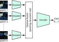
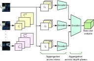
(a) Hartmann et al. [47].	(b) Flynn et al. [66].
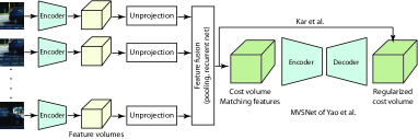
(c) Kar et al. [60] and Yao et al. [93].
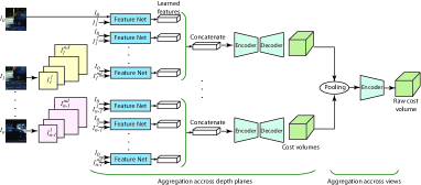
(d) Huang et al. [27].

Figure 6: Taxonomy of multivew stereo methods. (a), (b), and (c) perform early fusion, while (d) performs early fusion by aggregating features across depth plans, and late fusion by aggregating cost volumes across views.

Multiview Stereo (MVS) methods follow the same pipeline as of depth-from-stereo. Early works focused on computing the similarity between multiple patches. For instance, Hartmann et al. [47] (Fig. 6-(a)) replace the pairwise correlation layer used in stereo matching by an average pooling layer to aggregate the learned features of $n\geq 2$ input patches, and then feed the output to a top network, which returns a matching score. With this method, computing the best match for a pixel on the reference image requires $n_{d}^{n-1}$ forward passes. ($n_{d}$ is the number of depth levels and $n$ is the number of images.) This is computationally very expensive especially when dealing with high resolution images.

Techniques that compute depth maps in a single forward pass differ in the way the information from the multiple views is fed to the network and aggregated. We classify them into whether they are volumetric (Section 6.1) or Plane-Sweep Volume (PSV)-based (Section 6.2). The latter does not rely on intermediate volumetric representations of the 3D geometry. The only exception is the approach of Hou et al. [115], which performs temporal fusion of the latent representations of the input images. The approach, however, requires temporally-ordered images. Table IV provides a taxonomy and compares $13$ state-of-the-art MVS techniques.

6.1 Volumetric representations

One of the main issues for MVS reconstruction is how to match, in an efficient way, features across multiple images. Pairwise stereo methods rectify the images so that the search for correspondences is restricted to the horizontal epipolar lines. This is not possible with MVS due to the large view angle differences between the images. This has bee addressed using volumetric representations of the scene geometry [116, 60]. Depth maps are then generated by projection from the desired viewpoint. For a given input image, with known camera parameters, a ray from the viewpoint is cast through each image pixel. The voxels intersected by that ray are assigned the color [116] or the learned feature [60] of that pixel. Existing methods differ in the way information from multiple views are fused:

(1) Fusing feature grids. Kar et al. [60] (Fig. 6-(c)) fuse, recursively, the back-projected 3D feature grids using a recurrent neural network (RNN). The produced 3D grid is regularized using an encoder-decoder. To avoid dependency on the order of the images, Kar et al. [60] randomly permute the input images during training while constraining the output to be the same.

(2) Fusing pairwise cost volumes. Choi et al. [117] fuse the cost volumes, computed from each pair of images, using a weighted sum where the weight of each volume is the confidence map computed from that cost volume.

(3) Fusing the reconstructed surfaces. Ji et al. [116] process each pair of volumetric grids using a 3D CNN, which classifies whether a voxel is a surface point or not. To avoid the exhaustive combination of every possible image pairs, Ji et al. [116] learn their relative importance, using a network composed of fully-connected layers, automatically select a few view pairs based on their relative importance to reconstruct multiple volumetric grids, and take their weighted sum to produce the final 3D reconstruction.

To handle high resolution volumetric grids, Ji et al. [116] split the whole space into small Colored Voxel Cubes (CVCs) and regress the surface cube-by-cube. While this reduces the memory requirements, it requires multiple forward passes and thus increases the computation time. Paschalidou et al. [91] avoid the explicit use of the volumetric representation. Instead, each voxel of the grid is projected onto each of the input views, before computing the pairwise correlation between the corresponding learned features on each pair of views, and then averaging them over all pairs of views. Repeating this process for each depth value will result in the depth distribution on each pixel. This depth distribution is regularized using an MRF formulated as a differentiable function to enable end-to-end training.

In terms of performance, the volumetric approach of Ji et al. [116] requires $4$ hours to obtain a full reconstruction of a typical scene in DTU dataset [24]. The approach of Paschalidou et al. [91] takes approximately $25$mins, on an Intel i7 computer with an Nvidia GTX Titan X GPU, for the same task. Finally, methods that perform fusion post-reconstruction have higher reconstruction errors compared to those that perform early fusion.

6.2 Plane-Sweep Volume representations

These methods directly estimate depth maps from the input without using intermediate volumetric representations of the 3D geometry. As such, they are computationally more efficient. The main challenge to address is how to efficiently match features across multiple views in a single forward pass. This is done by using the Plane-Sweep Volumes (PSV) [66, 27, 118, 93, 119, 90], i.e., they back project the input images [66, 27, 118] or their learned features [93, 119, 90] into planes at different depth values, forming PSVs from which the depth map is estimated. Existing methods differ in the way the PSVs are processed with the feature extraction and feature matching blocks.

Flynn et al.’s network [66] (Fig. 6-(b)) is composed of $n_{d}$ branches, one for each depth plane. The $0pt-$th branch of the network takes as input the reference image and the planes of the PSVs of the other images which are located at depth $0pt$. These are packed together and fed to a two-stage network. The first stage computes matching features between the reference image and all the PSV planes located at depth $0pt$. The second stage models interactions across depth planes using convolutional layers. The final block of the network is a per-pixel softmax over depth, which returns the most probable depth value per pixel. The approach requires that the number of views and the camera parameters of each view to be known.

Huang et al. [27]’s approach (Fig. 6-(d)) starts with a pairwise matching step where a cost volume is computed between the reference image and each of the input images. For a given pair $(I_{1},I_{i}),i=2,\dots,n$, $I_{i}$ is first back-projected into a PSV. A siamese network then computes a matching cost volume between $I_{1}$ and each of the PSV planes. These volumes are aggregated into a single cost volume using an encoder-decoder network. This is referred to as intra-volume aggregation. Finally a max-pooling layer is used to aggregate the multi intra-volumes into a single inter-volume, which is then used to predict the depth map. Unlike Flynn et al. [66], Huang et al. [27]’s approach does not require a fixed number of input views since aggregation is performed using pooling. In fact, the number of views can vary between training and at runtime.

Unlike [66, 27], which back-project the input images, the MVSNet of Yao et al. [93] use the camera parameters to back-project the learned features into a 3D frustum of a reference camera sliced into parallel frontal planes, one for each depth value. The approach then generates the matching cost volume upon a pixel-wise variance-based metric, and finally a generic 3D U-Net is used to regularize the matching cost volume to estimate the depth maps. Luo et al. [119] extend MVSNet [93] to P-MVSNet in two ways. First, a raw cost volume is processed with a learnable patch-wise aggregation function before feeding it to the regularization network. This improves the matching robustness and accuracy for noisy data. Second, instead of using a generic 3D-UNet network for regularization, P-MVSNet uses a hybrid isotropic-anisotropic 3D-UNet. The plane-sweep volumes are essentially anisotropic in depth and spatial directions, but they are often approximated by isotropic cost volumes, which could be detrimental. In fact, one can infer the corresponding depth map along the depth direction of the matching cost volume, but cannot get the same information along other directions. Luo et al. [119] exploit this fact, through the proposed hybrid 3D U-Net with isotropic and anisotropic 3D convolutions, to guide the regularization of matching confidence volume.

The main advantage of using PSVs is that they eliminate the need to supply rectified images. In other words, the camera parameters are implicitly encoded. However, in order to compute the PSVs, the intrinsic and extrinsic camera parameters need to be either provided in advance or estimated using, for example, Structure-from-Motion techniques as in [27]. Also, these methods require setting in advance the disparity range and its discretisation. Moreover, they often result in a complex network architecture. Wang et al. [120] propose a light-weight architecture. It stacks together the reference image and the cost volume, computed using the absolute difference between the reference image and each other image but at different depth planes, and feeds them to an encoder-decoder network, with skip connections, to estimate the inverse depth at three different resolutions. Wang et al. [120] use a view selection rule, which selects the frames that have enough angle or translation difference and then use the selected frames to compute the cost volume.

Finally, note that feature back-projection has been also used by Won et al. [30] for omnidirectional depth estimation from a wide-baseline multi-view stereo setup. The approach uses spherical maps and spherical cost volumes.

TABLE IV: Taxonomy and comparison of $13$ deep learning-based MVS techniques.

Method	Year	Representation	Fusion	Training		Peformance on (DTU, SUN3D, ETH3D)					Complexity
						#images	Error ($mm$)	% $<1mm$	% $<2mm$		# Params	Memory	Complexity	Time (s)
Kar et al. [60]	2017	Volumetric	Recurrent fusion	Supervised		Variable	$-$	$-$	$-$		$-$	$-$	$-$	$-$
			of 3D feature grids
Hartmann et al. [47]	2017	Replace correlation by pooling		Supervised		$5$	$(1.356,-,-)$	$-$	$-$		$-$	$-$	$-$	$-$
						(can vary)
Ji et al. [116]	2017	Volumetric	Reconstructed surfaces	Supervised		$5$	$(0.745,-,-)$	$69.95$	$74.4$		$-$	$-$	$-$	$4$ hrs
Choi et al. [117]	2018	Volumetric	Pairwise cost volumes	Supervised		$5$	$(0.6511,-,-)$	$-$	$-$		$-$	$-$	$-$	$-$
Huang et al. [27]	2018	PSV	Encoder-decoder for intra-volume,	Supervised		Variable	$(-,0.419,0.412)$	$-$	$-$		$-$	$-$	$-$	$-$
			Max pooling for inter-volume
Leroy et al. [118]	2018	PSV	Depth fusion	Supervised		Variable	$(0.599,-,-)$	$-$	$-$		$72$K	$-$	$-$	$-$
Paschalidou et al. [91]	2018	Depth-based	Avg. pooling over	Supervised		Variable	$(-,-,-)$	$-$	$-$		$-$	$7$GB	$-$	$25$ mins
			pairwsie correlations
Yao et al. [93]	2018	PSV	Feature pooling by variance	Supervised		$5$	$(0.462,0.397,0.470)$	$75.69$	$80.25$		$363$K	$5.28$GB	$O(0pt\times 0pt\times n_{d})$	$0.9$s
Wang et al. [120]	2018	PSV and abs.	Concatenation of pairwise	Supervised		Variable	$(-,0.114,0.257)$	$-$	$-$		$33.9$M for	$-$	$-$	$0.04$
		difference	cost volumes and ref. image								$n_{d}=64$
Hou et al. [115]	2019	$-$	Temporal fusion of	Supervised		Variable	$(-,\textbf{0.101},0.229)$	$-$	$-$		$-$	$-$	$-$	$-$
			the latent rep.			(video sequence)
Luo et al. [119]	2019	PSV	Feature pooling by variance	Supervised		Variable	$(0.406,-,-)$	$-$	$-$		$-$	$-$	$-$	$-$
Xue et al.et al. [90]	2019	PSV	Cost volume	Supervised		$5$	$(\textbf{0.398},-,-)$	$80.02$	$83.84$		$571$K	$5.43$GB	$O(0pt\times 0pt\times n_{d})$	$1.8$s
			pooling by variance			(can vary)
Won et al. [30]	2019	Spherical PSV	Concatenation	Supervised		$-$	$-$	$-$	$-$		$-$	$-$	$-$	$-$

7 Training end-to-end stereo methods

The training process aims to find the network parameters $W$ that minimize a loss function $\mathcal{L}(W;\hat{D},\Theta)$ where $\hat{D}$ is the estimated disparity, and $\Theta$ are the supervisory cues. The loss function is defined as the sum of a data term $\mathcal{L}_{1}(\hat{D},\Theta,W)$, which measures the discrepancy between the ground-truth and the estimated disparity, and a regularization or smoothness term $\mathcal{L}_{2}(\hat{D},W)$, which imposes local or global constraints on the solution. The type of supervisory cues defines the degree of supervision (Section 7.1), which can be supervised with 3D groundtruth (Section 7.1.1), self-supervised using auxiliary cues (Section 7.1.2), or weakly supervised (Section 7.1.3). Some methods use additional cues, in the form of constraints on the solution, to boost the accuracy and performance (Section 7.2). One of the main challenges of deep learning-based techniques is their ability to generalize to new domains. Section 7.3 reviews methods that addressed this issue. Finally, Section 7.4 reviews methods that learn network architectures.

7.1 Supervision methods

7.1.1 3D supervision methods

Supervised methods are trained to minimise a loss function that measures the error between the ground truth disparity and the estimated disparity. It is of the form:

$$\mathcal{L}=\frac{1}{N}\sum C(x)H(C(x)-\epsilon)\mathcal{D}\left(\Phi(d_{x}),\Phi(\hat{d}_{x})\right),$$ (6)

where: $d_{x}$ a $\hat{d}_{x}$ are, respectively, the groundtruth and the estimated disparity at pixel $x$. $\mathcal{D}$ is a measure of distance, which can be the $L_{2}$, the $L_{1}$ [61, 121, 62, 99], the smooth $L_{1}$ [64], or the smooth $L_{1}$ but approximated using the two-parameter robust function $\rho(\cdot)$ [72, 122]. $C(x)\in[0,1]$ is the confidence of the estimated disparity at $x$. Setting $C(x)=1$ and the threshold $\epsilon=0,\forall x$ is equivalent to ignoring the confidence map. $H(x)$ is the heavyside function, which is equal to $1$ if $x\geq 0$, and $0$ otherwise. $\Phi(\cdot)$ is either the identify or the log function. The latter avoids overfitting the network to large disparities.

Some papers restrict the sum in Eqn. (6) to be over only the valid pixels or regions of interest, e.g., foreground or visible pixels [123], to avoid outliers. Other, e.g., Yao et al. [93], divide the loss into two parts, one over the initial disparity and the other one over the refined disparity. The overall loss is then defined as the weighted sum of the two losses.

7.1.2 Self-supervised methods

Self-supervised methods, originally used in optical flow estimation [124, 125], have been proposed as a possible solution in the absence of sufficient ground-truth training data. These methods mainly rely on image reconstruction losses, taking advantage of the projective geometry, and the spatial and temporal coherence when multiple images of the same scene are available. The rationale is that if the estimated disparity map is as close as possible to the ground truth, then the discrepancy between the reference image and any of the other images but unprojected using the estimated depth map onto the reference image, is also minimized. The general loss function is of the form:

$$\mathcal{L}=\frac{1}{N}\sum_{x}\mathcal{D}\left(\Phi\left(I_{ref}\right)(x)-\Phi\left(\tilde{I}_{ref}\right)(x)\right),$$ (7)

where $\tilde{I}_{ref}$, which is $I_{right}$ but unwarped onto $I_{ref}$ using the estimated disparity, and $\mathcal{D}$ is a measure of distance. The mapping function $\Phi$ can be:

• The identity [126, 127, 70, 68]. In this case, the loss of Eqn. (7) is called a photometric or image reconstruction loss.

• A mapping to the feature space [68], i.e., $\Phi\left(I_{ref}\right)=\textbf{f}$ where f is the learned feature map.

• The gradient of the image, i.e., $\Phi\left(I_{ref}\right)=\nabla I_{ref}$, which is less sensitive to variations in lighting and acquisition conditions than the photometric loss.

The distance $\mathcal{D}$ can be the $L_{1}$ or $L_{2}$ distance. Some papers [70] also use more complex metrics such as the structural dissimilarity [128] between patches in $I_{ref}$ and in $\tilde{I}_{ref}$.

While stereo-based supervision methods do not require ground-truth 3D labels, they rely on the availability of calibrated stereo pairs during training.

7.1.3 Weakly supervised methods

Supervised methods for disparity estimation can achieve promising results if trained on large quantities of ground truth depth data. However, manually obtaining ground-truth depth data is extremely difficult and expensive, and is prone to noise and inaccuracies. Weakly supervised methods rely on auxiliary signals to reduce the amount of manual labelling. In particular, Tonioni et al.[129] used as a supervisory signal the depth estimated using traditional stereo matching techniques to fine-tune depth estimation networks. Since such depth data can be sparse, noisy, and prone to errors, they propose a confidence-guided loss that penalizes ground-truth depth values that are deemed not reliable. It is defined using Eqn. (6) by setting $\mathcal{D}(\cdot)$ to be the $L_{1}$ distance, and $\epsilon>0$. Kuznietsov et al. [130] use sparse ground-truth depth for supervised learning, while enforcing the deep network to produce photo-consistent dense depth maps in a stereo setup using a direct image alignment/reprojection loss. These two methods rely on an ad-hoc disparity estimator. To avoid that, Zhou et al. [131] propose an iterative approach, which starts with a randomly initialized network. At each iteration, it computes matches from the left to the right images, and matches from the right to the left images. It then selects the high confidence matches and adds them as labelled data for further training in the subsequent iterations. The confidence is computed using the left-right consistency of Eqn. (12).

7.2 Incorporating additional cues

Several works incorporate additional cues and constraints to improve the quality of the disparity estimates. Examples include smoothness [70], left-right consistency [70], maximum depth [70], and scale-invariant gradient loss [121]. Such cues can also be in the form of auxiliary information such as semantic cues used to guide the disparity estimation network. Below, we discuss a number of these works.

(1) Smoothness. In general, one can assume that neighboring pixels have similar disparity values. Such smoothness constraint can be enforced by minimizing:

• The absolute difference between the disparity predicted at $x$ and those predicted at each pixel $y$ within a certain predefined neighborhood $\mathcal{N}_{x}$ around $x$:

  $$\mathcal{L}=\frac{1}{N}\sum_{x}\sum_{y\in\mathcal{N}_{x}}|d_{x}-d_{y}|.$$ (8)

  Here, $N$ is the total number of pixels.

• The magnitude of the first-order gradient $\nabla$ of the estimated disparity map [68]:

  $$\small{\mathcal{L}=\frac{1}{N}\sum_{x}\left\{(\nabla_{u}d_{x})+(\nabla_{v}d_{x})\right\},x=(u,v).}$$ (9)

• The magnitude of the second-order gradient of the estimated disparity [127, 132]:

  $$\mathcal{L}=\frac{1}{N}\sum_{x}\left\{(\nabla_{u}^{2}d_{x})^{2}+(\nabla_{v}^{2}d_{x})^{2}\right\}.$$ (10)

• The second-order gradient of the estimated disparity map weighted by the image’s second-order gradients [70]:

$$\small{\mathcal{L}=\frac{1}{N}\sum_{x}\left\{|\nabla_{u}^{2}d_{x}|e^{-|\nabla_{u}^{2}I(x)|}+|\nabla_{v}^{2}d_{x}|e^{-|\nabla_{v}^{2}I(x)|}\right\}.}$$ (11)

(2) Consistency. Zhong et al. [70] introduced the loop-consistency loss, which is constructed as follows. Consider the left image $I_{left}$ and the synthesized image $\tilde{I}_{left}$ obtained by warping the right image to the left image coordinate using the disparity map defined on the right image. A second synthesized left image $\tilde{\tilde{I}}_{left}$ can also be generated by warping the left image to the right image coordinates, by using the disparities at the left image, and then warping it back to the left image using the disparity at the right image. The three versions of the left image provide two constraints: $I_{left}=\tilde{I}_{left}$ and $I_{left}=\tilde{\tilde{I}}_{left}$, which can be used to regularize the disparity maps. Godard et al. [133] introduce the left-right consistency term, which is a linear approximation of the loop consistency. The loss attempts to make the left-view disparity map equal to the projected right-view disparity map. It is defined as:

$$\mathcal{L}=\frac{1}{N}\sum_{x}|d_{x}-\tilde{d}_{x}|,$$ (12)

where $\tilde{d}$ is the disparity at the right image but reprojected onto the coordinates of the left image.

(3) Maximum-depth heuristic. There may be multiple warping functions that achieve a similar warping loss, especially for textureless areas. To provide strong regularization in these areas, Zhong et al. [70] use the Maximum-Depth Heuristic (MDH) [134] defined as the sum of all depths/disparities:

$$\mathcal{L}=\frac{1}{N}\sum_{x}|d_{x}|.$$ (13)

(4) Scale-invariant gradient loss [121]. It is defined as:

$$\mathcal{L}=\sum_{h\in A}\sum_{x}\|g_{h}[D](x)-g_{h}[\hat{D}](x)\|_{2},$$ (14)

where $A=\{1,2,4,8,16\}$, $x=(i,j)$, $f_{i,j}\equiv f(i,j)$, and

$$\small{g_{h}[f](i,j)=\left(\frac{f_{i+h,j}-f_{i,j}}{|f_{i+h,j}-f_{i,j}|},\frac{f_{i,j+h}-f_{i,j}}{|f_{i,j+h}-f_{i,j}|}\right)^{\top}.}$$ (15)

This loss penalizes relative depth errors between neighbouring pixels. This loss stimulates the network to compare depth values within a local neighbourhood for each pixel. It emphasizes depth discontinuities, stimulates sharp edges, and increases smoothness within homogeneous regions.

(5) Incorporating semantic cues. Some papers incorporate additional cues such as normal [135], segmentation [68], and edge [76] maps, to guide the disparity estimation. These can be either provided at the outset, e.g., estimated with a separate method as in [76], or estimated jointly with the disparity map. Qi et al. [135] propose a mechanism that uses the depth map to refine the quality of the normal estimates, and the normal map to refine the quality of the depth estimates. This is done using a two-stream network: a depth-to-normal network for normal map refinement using the initial depth estimates, and a normal-to-depth network for depth refinement using the estimated normal map.

Yang et al. [68] and Song et al. [76] incorporate semantics by stacking semantic maps (segmentation masks in the case of [68] and edge features in the case of [76]) with the 3D cost volume. Yang et al. [68] train jointly a disparity estimation network and a segmentation network by using a loss function defined as a weighted sum of the reconstruction error, a smoothness term, and a segmentation error. Song et al. [76] further incorporate edge cues in the edge-aware smoothness loss to penalize drastic depth changes in flat regions. Also, to allow for depth discontinuities at object boundaries, the edge-aware smoothness loss is defined based on the gradient map obtained from the edge detection sub-network, which is more semantically meaningful than the variation in raw pixel intensities.

Wu et al. [79] introduced an approach that fuses multiscale 4D cost volumes with semantic features obtained using a segmentation sub-network. The approach uses the features of the left and the right images as input to a semantic segmentation network similar to PSPNet [136]. Semantic features for each image are then obtained from the output of the classification layer of the segmentation network. A 4D semantic cost volume is obtained by concatenating each unary semantic feature with their corresponding unary from the opposite stereo image across each disparity level. Both the spatial pyramid cost volumes and the semantic cost volume are fed into a 3D multi-cost aggregation module, which aggregates them, using an encoder-decoder followed by a 3D feature fusion module, into a single 3D cost volume in a pairwise manner starting with the smallest volume.

In summary, appending semantic features to the cost volume improves the reconstruction of fine details, especially near object boundaries.

7.3 Domain adaptation and transfer learning

Deep architectures for depth estimation are severely affected by the domain shift issue, which hinders their effectiveness when performing inference on images significantly diverse from those used during the training stage. This can be observed, for instance, when moving between indoor and outdoor environments, from synthetic to real data, see Fig. 7, or between different outdoor/indoor environments, and when changing the camera model/parameters. As such, deep learning networks trained on one domain, e.g., by using synthetic data, suffer when applied to another domain, e.g., real data, resulting in blurry object boundaries and errors in ill-posed regions such as object occlusions, repeated patterns, and textureless regions. These are referred to as generalization glitches [137].

Several strategies have been proposed to adress this domain bias issue. They can be classified into two categories: adaptation by fine-tuning (Section 7.3.1) and adaptation by data transformation (Section 7.3.2). In both cases, the adaptation can be offline or online.

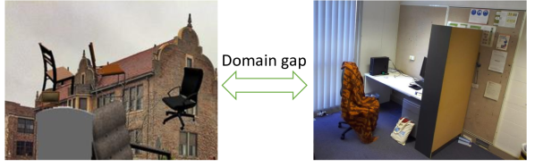
Figure 7: Illustration of the domain gap between synthetic (left) and real (right) images. The left image is from the FlyingThings synthetic dataset [22].

7.3.1 Adaptation by fine-tuning

Methods in this category perform domain adaptation by first training a network on images from a certain domain, e.g., synthetic images as in [22], and then fine-tuning it on images from a target domain. A major difficulty is to collect accurate ground-truth depth for stereo or multiview images from the target domain. Relying on active sensors (e.g., LiDAR) to obtain such supervised labeled data is not feasible in practical applications. As such, recent works, e.g.,  [129, 138, 137] rely on off-the-shelf stereo algorithms to obtain ground-truth disparity/depth labels in an unsupervised manner, together with state-of-the-art confidence measures to ascertain the correctness of the measurements of the off-the-shelf stereo algorithms. The latter is used in [129, 138] to discriminate between reliable and unreliable disparity measurements, to select the former and fine tune a pre-trained model, e.g., DispNet [22], using such smaller and sparse set of points as if they were ground-truth labels.

Pang et al. [137] also use a similar approach as in [129, 138] to address the generalization glitches. The approach, however, exploits the scale diversity, i.e., up-sampling the stereo pairs enables the model to perform stereo matching in a localized manner with subpixel accuracy, by performing iterative optimisation of predictions obtained at multiple resolutions of the input.

Note that self-supervised and weakly supervised techniques for disparity estimation, e.g.,  [139, 133, 140, 141] can also be used for offline domain adaptation. In particular, if stereo pairs of the target domain are available, these techniques can be fine-tuned, in an unsupervised manner, using reprojection losses, see Sections 7.1.2 and 7.1.3.

Although effective, these offline adaptation techniques reduce the usability of the methods since users are required to train the models every time they are exposed to a new domain. As a result, several recent papers developed online adaptation techniques. For example, Tonioni et al. [84] address the domain shift issue by casting adaptation as a continuous learning process whereby a stereo network can evolve online based on the images gathered by the camera during its real deployment. This is achieved in an unsupervised manner by computing error signals on the current frames, updating the whole network by a single back-propagation iteration, and moving to the next pair of input frames. To keep a high enough frame rate, Tonioni et al. [84] propose a lightweight, fast, and modular architecture, called MADNet, which allows training sub-portions of the whole network independently from each other. This allows adapting disparity estimation networks to unseen environments without supervision at approximately $25$ fps, while achieving an accuracy comparable to DispNetC [22]. Similarly, Zhong et al. [142] use video sequences to train a deep network online from a random initialization. They employ an LSTM in their model to leverage the temporal information during the prediction.

Zhong et al. [142] and Tonioni et al. [84] consider online adaptation separately from the initial training. Tonioni et al. [143], on the other hand, incorporate the adaptation procedure to the learning objective to obtain a set of initial parameters that are suitable for online adaptation, i.e., they can be adapted quickly to unseen environments. This is implemented using the model agnostic meta-learning framework of [144], an explicit learn-to-adapt framework that enables stereo methods to adapt quickly and continuously to new target domains in an unsupervised manner.

7.3.2 Adaptation by data transformation

Methods in this category transform the data of one domain to look similar in style to the data of the other domain. For example, Atapour-Abarghoue et al. [145] proposed a two-staged approach. The first stage trains a depth estimation model using synthetic data. The second stage is trained to transfer the style of synthetic images to real-world images. By doing so, the style of real images is first transformed to match the style of synthetic data and then fed into the depth estimation network, which has been trained on synthetic data. Zheng et al. [146] perform the opposite by transforming the synthetic images to become more realistic and using them to train the depth estimation network. Zhao et al. [147] consider both synthetic-to-real [146] and real-to-synthetic [148, 145] translations. The two translators are trained in an adversarial manner using an adversarial loss and a cycle-consistency loss. That is, a synthetic image when converted to a real image and converted back to the synthetic domain should look similar to the original one.

Although these methods have been used for monocular depth estimation, they are applicable to (multi-view) stereo matching methods.

7.4 Learning the network architecture

Much research work in depth estimation is being spent on manually optimizing network architectures, but what about if the optimal network architecture, along with its parameters, could be also learnt from data? Saika et al. [149] show how to use and extend existing AutoML techniques [150] to efficiently optimize large-scale U-Net-like encoder-decoder architectures for stereo-based depth estimation. Traditional AutoML techniques have extreme computational demand limiting their usage to small-scale classification tasks. Saika et al. [149] applies Differentiable Architecture Search (DARTs) [151] to encoder-decoder architectures. Its main idea is to have a large network that includes all architectural choices and to select the best parts of this network by optimization. This can be relaxed to a continuous optimization problem, which, together with the regular network training, leads to a bilevel optimization problem. Experiments conducted on DispNet of [75], an improved version of [22], show that the automatically optimized DispNet (AutoDispNet) yields better performance compared to the baseline DispNet of [75], with about the same number of parameters. The paper also shows that the benefits of automated optimization carry over to large stacked networks.

8 Discussion and comparison

Tables III and IV, respectively, compare the performance of the methods surveyed in this article on standard datasets such as KITTI2015 for pairwise stereo methods, and DTU, SUN3D and ETH3D for multiview stereo methods. Most of these methods have been trained on subsets of these publicly available datasets. A good disparity estimation method, once properly trained, should achieve good performance not only on publicly available benchmarks but on arbitrary novel images. They should not require re-training or fine-tuning every time the domain of usage changes. In this section, we will look at how some of these methods perform on novel unseen images. We will first describe in Section 8.1 the evaluation protocol, the images that will be used, and the evaluation metrics. We then discuss the performance of these methods in Sections 8.2 and 8.3.

8.1 Evaluation protocol

We consider several key methods and evaluate their performance on the stereo subset of the ApolloScape dataset [34], and on an in-house collected set of four images. The motivation behind this choice is two-fold. First, the ApolloScape dataset is composed of stereo images taken outdoor in autonomous driving setups. Thus, it exhibits several challenges related to uncontrolled complex and varying lighting conditions, and heavy occlusions. Second, the dataset is novel and existing methods have not been trained or exposed to this dataset. Thus, it can be used to assess how these methods generalize to novel scenarios. In this dataset, ground truth disparities have been acquired by accumulating 3D point clouds from Lidar and fitting 3D CAD models to individually moving cars. We also use four in-house images of size $0pt=640$ and $0pt=480$, see Fig. 9, specifically designed to challenge these methods. Two of the images are of real scenes: a Bicycles scene composed of bicycles in a parking, and an indoor Desk scene composed of office furnitures. We use a moving stereo camera to capture multiple stereo pairs, and Structure-from-Motion (SfM) to build a 3D model of the scenes. We then render depth maps from the real cameras’ viewpoints. Regions where depth is estimated with high confidence will be used as ground-truth. The remaining two images are synthetic, but real-looking. They include objects with complex structures, e.g., thin structures such as plants, large surfaces with either uniform colors or textures and repetitive patterns, presenting several challenges to stereo-based depth estimation algorithms.

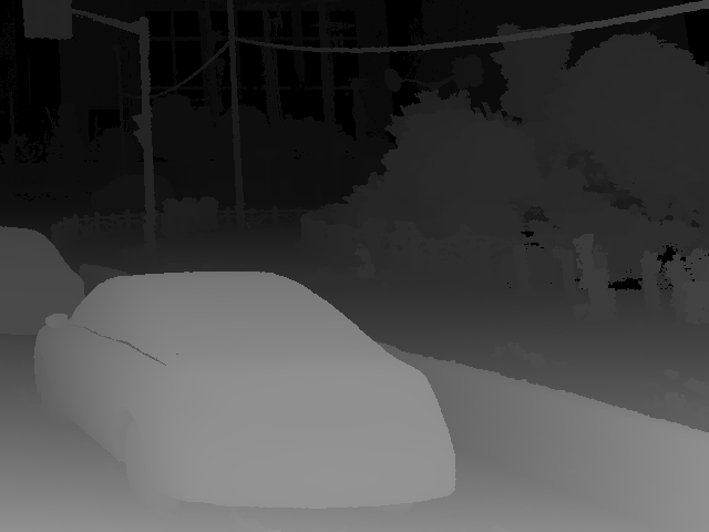
(a) Baseline: images with good lighting conditions.
(b) Challenge: images with challenging lighting conditions.

Figure 8: Examples of stereo pairs and their ground-truth disparity maps from the ApolloScape dataset [34].

(a) Left image.
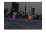
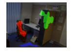
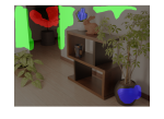
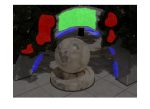
(b) Highlights of regions of interest where ground-truth disparity is
estimated with high confidence.
(c) Right image.
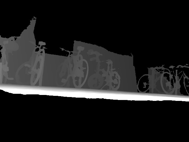
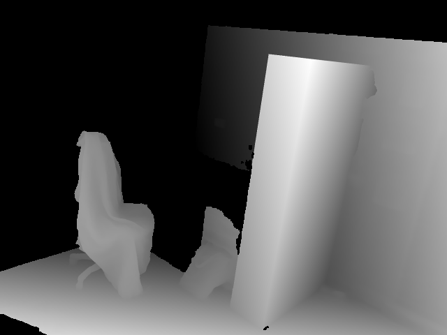
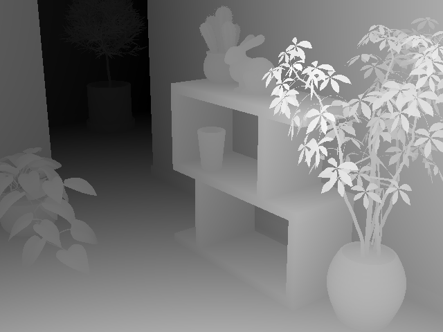
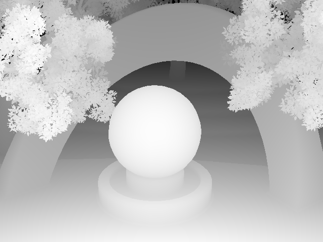
Disp. $\in[9.3,34.0]$	Disp. $\in[18.7,29.9]$	Disp. $\in[5.6,14.5]$	Disp. $\in[5.5,13.2]$
Depth $\in[2.1,7.8]$	Depth $\in[2.4,3.3]$	Depth $\in[7.8,25.0]$	Depth $\in[10.8,25.6]$
(d) Ground-truth disparity maps.

Figure 9: Four images, collected in-house and used to test $16$ state-of-the-art methods. The green masks on some of the left images highlight the pixels where the ground-truth disparity is available. The disparity range is shown in pixels while the depth range is in meters.

We have tested $16$ stereo-based methods published in $9$ papers (between $2018$ and $2019$), see below. We use the network weights as provided by the authors.

(1) AnyNet [88]: It is a four-stages network, which builds 3D cost volumes in a coarse-to-fine manner. The first stage estimates a low resolution disparity map by searching on a small disparity range. The subsequent stages estimate refined disparity maps using residual learning.

(2) DeepPruner [83]: It combines deep learning with PatchMatch [101] to speed up inference by adaptively pruning out the potentially large search space for correspondences. Two variants have been proposed: DeepPruner (Best), which downsamples the cost volume by a factor of $4$, and DeepPruner (Fast), which downsamples it by a factor of $8$.

(3) DispNet3 [75], an improved version of DispNet [22] where occlusions and disparity maps are jointly estimated.

(4) GANet [85]: It replaces a large number of the 3D convolutional layers in the regularization block with (1) two 3D convolutional layers, (2) a semi-global aggregation layer (SGA), and (3) a local guided aggregation layer (LGA). SGA and LGA layers capture local and whole-image cost dependencies. They are meant to improve the accuracy in challenging regions such as occlusions, large textureless/reflective regions, and thin structures.

(5) HighResNet [32]: To refine both the spatial and the depth resolutions while operating on high resolution images, this method searches for correspondences incrementally using a coarse-to-fine hierarchy. Its hierarchical design also allows for anytime on-demand reports of disparity.

(6) PSMNet [64]: It progressively regularizes a low resolution 4D cost volume, estimated from a pyramid of features.

(7) iResNet [63]: The initial disparity and the learned features are used to calculate a feature constancy map, which measures the correctness of the stereo matching. The initial disparity map and the feature constancy map are then fed into a sub-network for disparity refinement.

(8) UnsupAdpt [129]: It is an unsupervised adaptation approach that enables fine-tuning without any ground-truth information. It first trains DispNet-Corr1D [22] using the KITTI 2012 training dataset and then adapts the network to KITTI2015 and Middlebury 2014.

(9) SegStereo [68]: It is an unsupervised disparity estimation method, which uses segmentation masks to guide the disparity estimation. Both segmentation and disparity maps are jointly estimated with an end-to-end network.

The methods (1) to (7) are supervised with ground-truth depth maps while the methods (8) and (9) are self-supervised. We compare their accuracy at runtime using the overall Root Mean Square Error (RMSE) defined as:

$$\text{RMSE}^{2}_{\text{linear}}={\frac{1}{N}\sum_{N}{|0pt_{i}-\hat{0}pt_{i}|}^{2}},$$ (16)

and the Bad-n error defined as the percentage of pixels whose estimated disparity deviates with more than $n$ pixels from the ground truth. We use $n\in\{0.5,1,2,3,4,5\}$. The Bad-n error considers the distribution and spread of the error and thus provides a better insight on the accuracy of the methods. In addition to accuracy, we also report the computation time and memory footprint at runtime.

8.2 Computation time and memory footprint

TABLE V: Computation time and memory consumption, at runtime, on images of size $640\times 480$. SegStereo [68] has been tested on a PC equipped with an Nvidia GeForce RTX 2080. The other methods have been tested on a PC equipped with an Nvidia Tesla K40 GPU with a 12 Go graphic memory. See the Supplementary Material for a visual representation.

Method	Supervision	Cost vol.	Time (s)	Memory (GB)	Training set	Baseline				Challenge
	mode					Bkg	Fg	Bkg$+$Fg		Bkg	Fg	Bkg$+$Fg
AnyNet [88]	Supervised	3D	$0.285$	0.232	KITTI2015	9.46	10.74	10.34		9.83	11.60	11.15
					KITTI2012	9.80	10.29	10.20		9.34	10.62	10.61
DeepPruner (Best) [83]	Supervised	3D	$8.430$	$8.845$	KITTI2012$+$2015	9.64	9.43	9.46		12.38	8.74	10.48
DeepPruner (Fast) [83]	Supervised	3D	$3.930$	$6.166$	KITTI2012$+$2015	9.56	9.90	9.94		8.74	9.75	9.86
DispNet3 [75]	Supervised	3D	$-$	$10.953$	CSS-ft-KITTI	9.68	9.62	9.70		8.38	11.00	11.11
					CSS-FlyingThings3D [22]	9.11	9.64	9.54		8.97	9.91	10.19
					css-FlyingThings3D [22]	9.29	9.98	9.87		9.66	10.34	10.61
GANet [85]	Supervised	4D	$8.336$	3.017	KITTI2015	9.55	9.38	9.39		9.37	9.50	9.89
					KITTI2012	9.98	10.29	10.25		10.69	10.95	11.55
HighResNet [32]	Supervised	4D	0.037	$0.474$	Middleburry [20], KITTI2015 [21],	9.47	9.91	9.94		8.58	9.64	9.78
					ETH3D [25], HR-VS [32]
PSMNet [64]	Supervised	4D	$1.314$	$1.900$	KITTI2015	9.88	9.81	9.80		10.10	9.42	9.93
					KITTI2012	10.17	10.24	10.29		10.66	10.33	11.00
iResNet [63]	Supervised	3D	$0.939$	$7.656$	KITTI2015	60.04	61.72	60.54		45.87	46.85	47.86
					ROB [152]	22.08	17.16	18.08		23.01	16.51	18.83
UnsupAdpt [129]	Self-supervised	3D	$-$	$-$	KITTI2012 adapted to KITTI2015	9.44	10.39	10.19		10.10	10.42	10.78
					Shadow-on-Truck	8.52	10.08	9.58		10.66	10.88	10.27
SegStereo [68]	Self-supervised	3D	$0.195$	$\sim 12.00$	CityScapes [23]	9.26	10.30	10.17		9.03	10.49	10.54

From Table V, we can distinguish three types of methods; slow methods, e.g., PSMNet [64], DeepPruner (Best) and (Fast) [83], and GANet [85], require more than $1$ second to estimate one disparity map. They also require between $3$GB and $10$GB (for DispNet3 [75]) of memory at runtime. As such, these methods are very hard to deploy on mobile platforms. Average-speed methods, e.g., AnyNet [88] and iResNet [63], produce a disparity map in around one second. Finally, fast methods, e.g., HighResNet [32], require less than $0.1$ seconds. In general, methods that use 3D cost volumes are faster and less memory demanding than those that use 4D cost volumes. There are, however, two exceptions: iResNet [63] and DeepPruner [83], which use 3D cost volumes but require a large amount of memory at runtime. While iResNet requires less than a second to process images of size $0pt=640,0pt=480$, since it uses 2D convolutions to regularize the cost volume, DeepPruner [83] requires more than $3$ seconds. We also observe that HighResNet [32], which uses 4D cost volumes but adopts a hierarchical approach to produce disparity on demand, is very efficient in terms of computation time as it only requires $37$ms, which is almost $8$ times faster than AnyNet [88], which uses 3D cost volumes. Note also that AnyNet [88] can run on mobile devices due to its memory efficiency.

8.3 Reconstruction accuracy

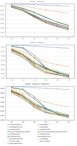
Figure 10: Overall Bad-n error, $n\in[0.5,5.0]$ on a selection of $141$ (baseline) images from the stereo vision challenge of ApolloScape dataset [34]. A similar behaviour is observed on the challenge subset, see the supplementary material. The horizontal axis is the error $n$ while the vertical axis is the percentage of pixels whose estimated disparity deviates with more than $n$ pixels from the ground truth.

Table V shows the average RMSE of each of the methods described in Section 8.1. We report the results on a baseline subset composed of $141$ images that look more or less like KITTI2012 images, hereinafter referred to as baseline, and on another subset composed of $33$ images with challenging lighting conditions, hereinafter referred to as challenge. Here, we focus on the relative comparison across methods since some of the high errors observed might be attributed to the way the ground-truth has been acquired in ApolloScape [34] dataset, rather than to the methods themselves.

We observe that these methods behave almost equally on the two subsets. However, the reconstruction error, is significantly important, $>8$ pixels, compared to the errors reported on standard datasets such as KITTI2012 and KITTI2015. This suggests that, when there is a significant domain gap between training and testing then the reconstruction accuracy can be significantly affected.

We also observe the same trend on the Bad-n curves of Fig. 10 where, in all methods, more than $25\%$ of the pixels had a reconstruction error that is larger than $5$ pixels. The Bad-n curves show that the errors are large on the foreground pixels, i.e., pixels that correspond to cars, with more than $55\%$ of the pixels having an error that is larger than $3$ pixels (against $35\%$ on the background pixels). Interestingly, Table V and Fig. 10 show that most of the methods achieve similar reconstruction accuracies. The only exception is iResNet [63] trained on Kitti2015 and on ROB [152], which had more than $90\%$, respectively $55\%$, of pixels with an error that is larger than $5$ pixels. In all methods, less than $5\%$ of the pixels had an error that is less than $2$ pixels. This suggests that achieving sub-pixel accuracy remains an important challenge for future research.

Note that SegStereo [68], which is self-supervised, achieves a similar or better performance than many of the supervised methods. Also, the unsupervised self-adaptation method of Tonioni et al. [129], which takes the baseline DispNet-Corr1D network [22] trained on KITTI 2012 and adapts it to KITTI2015 and Middlebury 2014, achieves one of the best performances on the foreground regions.

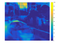
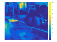
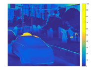
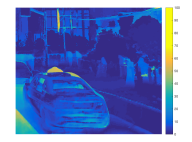
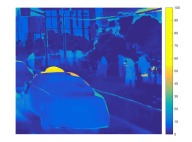
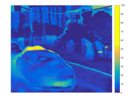
AnyNet (Kitti2012)	AnyNet (Kitti2015)	DeepPruner (fast)	DispNet3 (css)	GANet (Kittit2015)	Unsup.Adapt (Kitti)
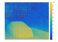
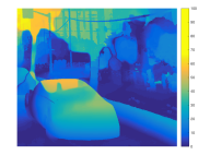
iResNet (Kitti2015)	iResNet (ROB)	PSMNet (Kitti2012)	PSMNet (Kitti2015)	SegStereo	Unsup.Adapt
					(shadowsontruck)
(a) Results on the images of Fig. 8-(a).
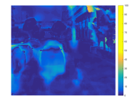
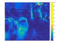
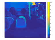
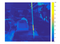
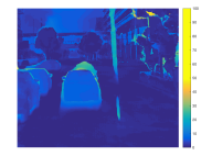
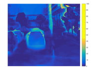
AnyNet (Kitti2012)	AnyNet (Kitti2015)	DeepPruner (fast)	DispNet3 (css)	GANet (Kittit2015)	Unsup.Adapt (Kitti)
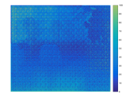
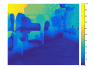
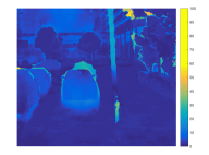
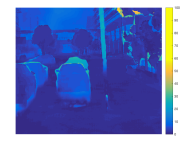
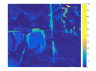
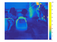
iResNet (Kitti2015)	iResNet (ROB)	PSMNet (Kitti2012)	PSMNet (Kitti2015)	SegStereo	Unsup.Adapt
					(shadowsontruck)
(b) Results on the images of Fig. 8-(b).

Figure 11: Pixel-wise errors between the ground-truth disparities and the disparities estimated from the images of Fig. 8.

In terms of the visual quality of the estimated disparities, see Fig. 11, we observe that most of the methods were able to recover the overall shape of trees but fail to reconstruct the details especially the leaves. The reconstruction errors are high in flat areas and around object boundaries. Also, highly reflective materials and poor lighting conditions remain a big challenge to these methods as shown in Fig. 11-(b). The supplementary material provides more results on the four stereo pairs of Fig. 9.

9 Future research directions

Deep learning methods for stereo-based depth estimation have achieved promising results. The topic, however, is still in its infancy and further developments are yet to be expected. In this section, we present some of the current issues and highlight directions for future research.

(1) Camera parameters. Most of the stereo-based techniques surveyed in this article require rectified images. Multi-view stereo techniques use Plane-Sweep Volumes or back-projected images/features. Both image rectification and PSVs require known camera parameters, which are challenging to estimate in the wild. Many papers attempted to address this problem for monocular depth estimation and for 3D shape reconstruction by jointly optimising for the camera parameters and the geometry of the 3D scene [153].

(2) Lighting conditions and complex material properties. Poor lighting conditions and complex materials properties remain a challenge to most of the current methods, see for example Fig. 11-(b). Combining object recognition, high-level scene understanding, and low-level feature learning can be one promising avenue to address these issues.

(3) Spatial and depth resolution. Most of the current techniques do not handle high resolution input images and generally produce depth maps of low spatial and depth resolution. Depth resolution is particularly limited, making the methods unable to reconstruct thin structures, e.g., vegetation and hair, and structures located at a far distance from the camera. Although refinement modules can improve the resolution of the estimated depth maps, the gain is still small compared to the resolution of the input images. This has recently been addressed using hierarchical techniques, which allow on-demand reports of disparity by capping the resolution of the intermediate results [32]. In these methods, low resolution depth maps can be produced in realtime, and thus can be used on mobile platforms, while high resolution maps would require more computation time. Producing, in realtime, accurate maps of high spatial and depth resolutions remains a challenge for future research.

(4) Realtime processing. Most deep learning methods for disparity estimation use 3D and 4D cost volumes, which are processed and regularized using 2D and 3D convolutions. They are expensive in terms of memory requirements and processing time. Developing lightweight, and subsequently fast, end-to-end deep networks remains a challenging avenue for future research.

(5) Disparity range. Existing techniques uniformly discretize the disparity range. This results in multiple issues. In particular, although the reconstruction error can be small in the disparity space, it can result in an error of meters in the depth space, especially at far ranges. One way to mitigate this is by discritizing disparity and depth uniformly in the log space. Also, changing the disparity range requires retraining the networks. Treating depth as a continuum could be one promising avenue for future research.

(6) Training. Deep networks heavily rely on the availability of training images annotated with ground-truth labels. This is very expensive and labor intensive for depth/disparity reconstruction. As such, the performance of the methods and their generalization ability can significantly be affected including the risk of overfitting the models to specific domains. Existing techniques mitigate this problem by either designing loss functions that do not require 3D annotations, or by using domain adaptation and transfer learning strategies. The former, however, requires calibrated cameras. Domain adaptation techniques, especially unsupervised ones [138], are recently attracting more attention since, with these techniques, one can train with both synthetic data, which are easy to obtain, and real-world data. They also adapt, in an unsupervised manner and at run-time to ever-changing environments as soon as new images are gathered. Early results are very encouraging and thus expect in the future to see the emergence of large datasets, similar to ImageNet but for 3D reconstruction.

(7) Automatically learning the network architecture, its activation functions, and its parameters from data. Most existing research has focused on designing novel network architectures and novel training methods for optimizing their parameters. It is only recently that some papers started to focus on automatically learning optimal architectures. Early attempts, e.g.,  [149], focus on simple architectures. We expect in the future to see more research on automatically learning complex disparity estimation architectures and their activation functions, using, for example, the neuro-evolution theory [154, 155], which will free the need for manual network design.

10 Conclusion

This paper provides a comprehensive survey of the recent developments in stereo-based depth estimation using deep learning techniques. Despite their infancy, these techniques are achieving state-of-the-art results. Since 2014, we have entered a new era where data-driven and machine learning techniques play a central role in image-based depth reconstruction. We have seen that, from $2014$ to $2019$, more than $150$ papers on the topic have been published in the major computer vision, computer graphics, and machine learning conferences and journals. Even during the final stages of this submission, more new papers are being published making it difficult to keep track of the recent developments, and more importantly, understand their differences and similarities, especially for new comers to the field. This timely survey can thus serve as a guide to the reader to navigate this fast-growing field of research.

Finally, there are several related topics that have not been covered in this survey. Examples include image-based 3D object reconstruction using deep learning, which has been recently surveyed by Han et al. [153], and monocular and video-based depth estimation, which requires a separate survey paper given the large amount of papers that have been published on the topic in the past $5$ to $6$ years. Other topics include photometric stereo and active stereo [156, 157], which are outside the scope of this paper.

Acknowledgements. We would like to thank all the authors of the reference papers who have made their codes and datasets publicly available. This work is supported in part by Murdoch University’s Vice Chancellor’s Small Steps of Innovation Funding Program, and by ARC DP150100294 and DP150104251.

Hamid Laga received the PhD degrees in Computer Science from Tokyo Institute of Technology in 2006. He is currently an Associate Professor at Murdoch University (Australia) and an Adjunct Associate Professor with the Phenomics and Bioinformatics Research Centre (PBRC) of the University of South Australia. His research interests span various fields of machine learning, computer vision, computer graphics, and pattern recognition, with a special focus on the 3D reconstruction, modeling and analysis of static and deformable 3D objects, and on image analysis and big data in agriculture and health. He is the recipient of the Best Paper Awards at SGP2017, DICTA2012, and SMI2006.

Laurent Valentin Jospin Laurent Valentin Jospin is a young research student in the field of computer vision. His main research interests include 3d reconstruction, sampling and image acquisition strategies, computer vision applied to robotic navigation and computer vision applied to environmental sciences. Holder of a master of science in environmental engineering from EPFL since 2017 with a thesis on accuracy prediction in aerial mapping, his research career started as intern in two EPFL labs, publishing his first three papers in the process, before starting a PhD in computer science at the University of Western Australia in 2019. His thesis project focus on real time 3D reconstruction with different computer vision techniques.

Faird Boussaid received the M.S. and Ph.D. degrees in microelectronics from the National Institute of Applied Science (INSA), Toulouse, France, in 1996 and 1999 respectively. He joined Edith Cowan University, Perth, Australia, as a Postdoctoral Research Fellow, and a Member of the Visual Information Processing Research Group in 2000. He joined the University of Western Australia, Crawley, Australia, in 2005, where he is currently a Professor. His current research interests include neuromorphic engineering, smart sensors, and machine learning.

Mohammed Bennamoun is Winthrop Professor in the Department of Computer Science and Software Engineering at UWA and is a researcher in computer vision, machine/deep learning, robotics, and signal/speech processing. He has published 4 books (available on Amazon, 1 edited book, 1 Encyclopedia article, 14 book chapters, 120+ journal papers, 250+ conference publications, 16 invited and keynote publications. His h-index is 47 and his number of citations is 10,000+ (Google Scholar). He was awarded 65+ competitive research grants, from the Australian Research Council, and numerous other Government, UWA and industry Research Grants. He successfully supervised +26 PhD students to completion. He won the Best Supervisor of the Year Award at QUT (1998), and received award for research supervision at UWA (2008 and 2016) and Vice-Chancellor Award for mentorship (2016). He delivered conference tutorials at major conferences, including: IEEE CVPR 2016, Interspeech 2014, IEEE ICASSP, and ECCV. He was also invited to give a Tutorial at an International Summer School on Deep Learning (DeepLearn 2017).

References

- [1] S. Khan, H. Rahmani, S. A. A. Shah, and M. Bennamoun, “A guide to convolutional neural networks for computer vision,” Synthesis Lectures on Computer Vision, vol. 8, no. 1, pp. 1–207, 2018.
- [2] B. Li, C. Shen, Y. Dai, A. Van Den Hengel, and M. He, “Depth and surface normal estimation from monocular images using regression on deep features and hierarchical CRFs,” in IEEE CVPR, 2015, pp. 1119–1127.
- [3] D. Eigen and R. Fergus, “Predicting depth, surface normals and semantic labels with a common multi-scale convolutional architecture,” in IEEE ICCV, 2015, pp. 2650–2658.
- [4] R. Garg, V. K. BG, G. Carneiro, and I. Reid, “Unsupervised CNN for single view depth estimation: Geometry to the rescue,” in ECCV, 2016, pp. 740–756.
- [5] F. Liu, C. Shen, G. Lin, and I. D. Reid, “Learning Depth from Single Monocular Images Using Deep Convolutional Neural Fields,” IEEE PAMI, vol. 38, no. 10, pp. 2024–2039, 2016.
- [6] J. Yang, S. E. Reed, M.-H. Yang, and H. Lee, “Weakly-supervised disentangling with recurrent transformations for 3D view synthesis,” in NIPS, 2015, pp. 1099–1107.
- [7] T. D. Kulkarni, W. F. Whitney, P. Kohli, and J. Tenenbaum, “Deep convolutional inverse graphics network,” in NIPS, 2015, pp. 2539–2547.
- [8] M. Tatarchenko, A. Dosovitskiy, and T. Brox, “Multi-view 3D models from single images with a convolutional network,” in ECCV, 2016, pp. 322–337.
- [9] T. Zhou, S. Tulsiani, W. Sun, J. Malik, and A. A. Efros, “View synthesis by appearance flow,” in ECCV, 2016, pp. 286–301.
- [10] E. Park, J. Yang, E. Yumer, D. Ceylan, and A. C. Berg, “Transformation-grounded image generation network for novel 3D view synthesis,” in IEEE CVPR, 2017, pp. 702–711.
- [11] D. Scharstein and R. Szeliski, “A taxonomy and evaluation of dense two-frame stereo correspondence algorithms,” IJCV, vol. 47, no. 1-3, pp. 7–42, 2002.
- [12] D. Eigen, C. Puhrsch, and R. Fergus, “Depth map prediction from a single image using a multi-scale deep network,” in NIPS, 2014, pp. 2366–2374.
- [13] X. Wang, D. Fouhey, and A. Gupta, “Designing deep networks for surface normal estimation,” in IEEE CVPR, 2015, pp. 539–547.
- [14] A. Saxena, M. Sun, and A. Y. Ng, “Make3d: Learning 3d scene structure from a single still image,” IEEE PAMI, vol. 31, no. 5, pp. 824–840, 2009.
- [15] A. Geiger, P. Lenz, and R. Urtasun, “Are we ready for autonomous driving? the kitti vision benchmark suite,” in IEEE CVPR, 2012, pp. 3354–3361.
- [16] D. J. Butler, J. Wulff, G. B. Stanley, and M. J. Black, “A naturalistic open source movie for optical flow evaluation,” in ECCV, 2012, pp. 611–625.
- [17] N. Silberman, D. Hoiem, P. Kohli, and R. Fergus, “Indoor segmentation and support inference from rgbd images,” ECCV, pp. 746–760, 2012.
- [18] J. Sturm, N. Engelhard, F. Endres, W. Burgard, and D. Cremers, “A benchmark for the evaluation of rgb-d slam systems,” in IROS, 2012, pp. 573–580.
- [19] J. Xiao, A. Owens, and A. Torralba, “Sun3d: A database of big spaces reconstructed using sfm and object labels,” in IEEE ICCV, 2013, pp. 1625–1632.
- [20] D. Scharstein, H. Hirschmüller, Y. Kitajima, G. Krathwohl, N. Nešić, X. Wang, and P. Westling, “High-resolution stereo datasets with subpixel-accurate ground truth,” in German conference on pattern recognition, 2014, pp. 31–42.
- [21] M. Menze and A. Geiger, “Object scene flow for autonomous vehicles,” in IEEE CVPR, 2015, pp. 3061–3070.
- [22] N. Mayer, E. Ilg, P. Hausser, P. Fischer, D. Cremers, A. Dosovitskiy, and T. Brox, “A large dataset to train convolutional networks for disparity, optical flow, and scene flow estimation,” in IEEE CVPR, 2016, pp. 4040–4048.
- [23] M. Cordts, M. Omran, S. Ramos, T. Rehfeld, M. Enzweiler, R. Benenson, U. Franke, S. Roth, and B. Schiele, “The cityscapes dataset for semantic urban scene understanding,” in IEEE CVPR, 2016, pp. 3213–3223.
- [24] H. Aanæs, R. R. Jensen, G. Vogiatzis, E. Tola, and A. B. Dahl, “Large-scale data for multiple-view stereopsis,” IJCV, vol. 120, no. 2, pp. 153–168, 2016.
- [25] T. Schöps, J. L. Schönberger, S. Galliani, T. Sattler, K. Schindler, M. Pollefeys, and A. Geiger, “A multi-view stereo benchmark with high-resolution images and multi-camera videos,” in IEEE CVPR, 2017, pp. 3260–3269.
- [26] S. Song, F. Yu, A. Zeng, A. X. Chang, M. Savva, and T. Funkhouser, “Semantic scene completion from a single depth image,” in IEEE CVPR, 2017, pp. 1746–1754.
- [27] P.-H. Huang, K. Matzen, J. Kopf, N. Ahuja, and J.-B. Huang, “DeepMVS: Learning Multi-view Stereopsis,” in IEEE CVPR, 2018, pp. 2821–2830.
- [28] Z. Li and N. Snavely, “MegaDepth: Learning Single-View Depth Prediction From Internet Photos,” in IEEE CVPR, 2018, pp. 2041–2050.
- [29] J. Jeon and S. Lee, “Reconstruction-based Pairwise Depth Dataset for Depth Image Enhancement Using CNN,” in ECCV, 2018, pp. 422–438.
- [30] C. Won, J. Ryu, and J. Lim, “OmniMVS: End-to-End Learning for Omnidirectional Stereo Matching,” in IEEE ICCV, 2019, pp. 8987–8996.
- [31] ——, “End-to-End Learning for Omnidirectional Stereo Matching with Uncertainty Prior,” IEEE PAMI, 2020.
- [32] G. Yang, J. Manela, M. Happold, and D. Ramanan, “Hierarchical Deep Stereo Matching on High-Resolution Images,” in IEEE CVPR, 2019, pp. 5515–5524.
- [33] G. Yang, X. Song, C. Huang, Z. Deng, J. Shi, and B. Zhou, “Drivingstereo: A large-scale dataset for stereo matching in autonomous driving scenarios,” in IEEE CVPR, 2019, pp. 899–908.
- [34] P. Wang, X. Huang, X. Cheng, D. Zhou, Q. Geng, and R. Yang, “The apolloscape open dataset for autonomous driving and its application,” IEEE transactions on pattern analysis and machine intelligence, 2019.
- [35] J. Geyer, Y. Kassahun, M. Mahmudi, X. Ricou, R. Durgesh, A. S. Chung, L. Hauswald, V. H. Pham, M. Mühlegg, S. Dorn et al., “A2d2: Audi autonomous driving dataset,” arXiv preprint arXiv:2004.06320, 2020.
- [36] N. Mayer, E. Ilg, P. Fischer, C. Hazirbas, D. Cremers, A. Dosovitskiy, and T. Brox, “What makes good synthetic training data for learning disparity and optical flow estimation?” International Journal of Computer Vision, vol. 126, no. 9, pp. 942–960, 2018.
- [37] S. Zagoruyko and N. Komodakis, “Learning to compare image patches via convolutional neural networks,” in IEEE CVPR, 2015, pp. 4353–4361.
- [38] X. Han, T. Leung, Y. Jia, R. Sukthankar, and A. C. Berg, “MatchNet: Unifying feature and metric learning for patch-based matching,” in IEEE CVPR, 2015, pp. 3279–3286.
- [39] J. Zbontar and Y. LeCun, “Computing the stereo matching cost with a convolutional neural network,” in IEEE CVPR, 2015, pp. 1592–1599.
- [40] W. Chen, X. Sun, L. Wang, Y. Yu, and C. Huang, “A deep visual correspondence embedding model for stereo matching costs,” in IEEE ICCV, 2015, pp. 972–980.
- [41] E. Simo-Serra, E. Trulls, L. Ferraz, I. Kokkinos, P. Fua, and F. Moreno-Noguer, “Discriminative learning of deep convolutional feature point descriptors,” in IEEE ICCV, 2015, pp. 118–126.
- [42] J. Zbontar and Y. LeCun, “Stereo matching by training a convolutional neural network to compare image patches,” Journal of Machine Learning Research, vol. 17, no. 1-32, p. 2, 2016.
- [43] V. Balntas, E. Johns, L. Tang, and K. Mikolajczyk, “PN-Net: Conjoined Triple Deep Network for Learning Local Image Descriptors,” CoRR, 2016.
- [44] W. Luo, A. G. Schwing, and R. Urtasun, “Efficient deep learning for stereo matching,” in IEEE CVPR, 2016, pp. 5695–5703.
- [45] B. Kumar, G. Carneiro, I. Reid et al., “Learning local image descriptors with deep siamese and triplet convolutional networks by minimising global loss functions,” in IEEE CVPR, 2016, pp. 5385–5394.
- [46] A. Shaked and L. Wolf, “Improved stereo matching with constant highway networks and reflective confidence learning,” in IEEE CVPR, 2017, pp. 4641–4650.
- [47] W. Hartmann, S. Galliani, M. Havlena, L. Van Gool, and K. Schindler, “Learned multi-patch similarity,” in IEEE ICCV, 2017, pp. 1595–1603.
- [48] H. Park and K. M. Lee, “Look wider to match image patches with convolutional neural networks,” IEEE Signal Processing Letters, vol. 24, no. 12, pp. 1788–1792, 2017.
- [49] X. Ye, J. Li, H. Wang, H. Huang, and X. Zhang, “Efficient stereo matching leveraging deep local and context information,” IEEE Access, vol. 5, pp. 18 745–18 755, 2017.
- [50] S. Tulyakov, A. Ivanov, and F. Fleuret, “Weakly supervised learning of deep metrics for stereo reconstruction,” in IEEE ICCV, 2017, pp. 1339–1348.
- [51] A. Dosovitskiy, P. Fischer, E. Ilg, P. Hausser, C. Hazirbas, V. Golkov, P. Van Der Smagt, D. Cremers, and T. Brox, “FlowNet: Learning optical flow with convolutional networks,” in IEEE ICCV, 2015, pp. 2758–2766.
- [52] H. Fu, M. Gong, C. Wang, K. Batmanghelich, and D. Tao, “Deep Ordinal Regression Network for Monocular Depth Estimation,” in IEEE CVPR, June 2018.
- [53] S. Sukhbaatar and R. Fergus, “Learning from noisy labels with deep neural networks,” ICLR Workshop, 2014.
- [54] P. Fischer, A. Dosovitskiy, and T. Brox, “Descriptor matching with convolutional neural networks: a comparison to sift,” CoRR, 2014.
- [55] H. Hirschmuller, “Stereo processing by semiglobal matching and mutual information,” IEEE PAMI, vol. 30, no. 2, pp. 328–341, 2008.
- [56] A. Seki and M. Pollefeys, “SGM-Nets: Semi-global matching with neural networks,” in IEEE CVPR Workshops, 2017, pp. 21–26.
- [57] J. L. Schönberger, S. N. Sinha, and M. Pollefeys, “Learning to Fuse Proposals from Multiple Scanline Optimizations in Semi-Global Matching,” in Proceedings of ECCV, 2018, pp. 739–755.
- [58] M. Poggi and S. Mattoccia, “Learning a general-purpose confidence measure based on o(1) features and a smarter aggregation strategy for semi global matching,” in 3DV, 2016, pp. 509–518.
- [59] X. Hu and P. Mordohai, “A quantitative evaluation of confidence measures for stereo vision,” IEEE PAMI, vol. 34, no. 11, pp. 2121–2133, 2012.
- [60] A. Kar, C. Häne, and J. Malik, “Learning a multi-view stereo machine,” in NIPS, 2017, pp. 364–375.
- [61] A. Kendall, H. Martirosyan, S. Dasgupta, P. Henry, R. Kennedy, A. Bachrach, and A. Bry, “End-to-end learning of geometry and context for deep stereo regression,” IEEE ICCV, pp. 66–75, 2017.
- [62] J. Pang, W. Sun, J. S. Ren, C. Yang, and Q. Yan, “Cascade residual learning: A two-stage convolutional neural network for stereo matching,” in ICCV Workshops, vol. 7, no. 8, 2017.
- [63] Z. Liang, Y. Feng, Y. G. H. L. W. Chen, and L. Q. L. Z. J. Zhang, “Learning for Disparity Estimation Through Feature Constancy,” in IEEE CVPR, 2018, pp. 2811–2820.
- [64] J. Chang and Y. Chen, “Pyramid Stereo Matching Network,” IEEE CVPR, pp. 5410–5418, 2018.
- [65] G.-Y. Nie, M.-M. Cheng, Y. Liu, Z. Liang, D.-P. Fan, Y. Liu, and Y. Wang, “Multi-Level Context Ultra-Aggregation for Stereo Matching,” in IEEE CVPR, 2019, pp. 3283–3291.
- [66] J. Flynn, I. Neulander, J. Philbin, and N. Snavely, “DeepStereo: Learning to predict new views from the world’s imagery,” in IEEE CVPR, 2016, pp. 5515–5524.
- [67] K. He, X. Zhang, S. Ren, and J. Sun, “Deep residual learning for image recognition,” in IEEE CVPR, 2016, pp. 770–778.
- [68] G. Yang, H. Zhao, J. Shi, Z. Deng, and J. Jia, “SegStereo: Exploiting semantic information for disparity estimation,” in ECCV, 2018, pp. 636–651.
- [69] F. Yu, D. Wang, E. Shelhamer, and T. Darrell, “Deep layer aggregation,” in IEEE CVPR, 2018, pp. 2403–2412.
- [70] Y. Zhong, Y. Dai, and H. Li, “Self-supervised learning for stereo matching with self-improving ability,” arXiv:1709.00930, 2017.
- [71] P. Knöbelreiter, C. Reinbacher, A. Shekhovtsov, and T. Pock, “End-to-end training of hybrid CNN-CRF models for stereo,” in IEEE CVPR, 2017, pp. 1456–1465.
- [72] S. Khamis, S. Fanello, C. Rhemann, A. Kowdle, J. Valentin, and S. Izadi, “StereoNet: Guided hierarchical refinement for real-time edge-aware depth prediction,” ECCV, 2018.
- [73] Y. Zhang, S. Khamis, C. Rhemann, J. Valentin, A. Kowdle, V. Tankovich, M. Schoenberg, S. Izadi, T. Funkhouser, and S. Fanello, “ActiveStereoNet: end-to-end self-supervised learning for active stereo systems,” ECCV, pp. 784–801, 2018.
- [74] Z. Jie, P. Wang, Y. Ling, B. Zhao, Y. Wei, J. Feng, and W. Liu, “Left-Right Comparative Recurrent Model for Stereo Matching,” in IEEE CVPR, 2018, pp. 3838–3846.
- [75] E. Ilg, T. Saikia, M. Keuper, and T. Brox, “Occlusions, Motion and Depth Boundaries with a Generic Network for Disparity, Optical Flow or Scene Flow Estimation,” in ECCV, 2018, pp. 614–630.
- [76] X. Song, X. Zhao, H. Hu, and L. Fang, “EdgeStereo: A Context Integrated Residual Pyramid Network for Stereo Matching,” ACCV, 2018.
- [77] L. Yu, Y. Wang, Y. Wu, and Y. Jia, “Deep Stereo Matching with Explicit Cost Aaggregation Sub-architecture,” AAAI, 2018.
- [78] S. Tulyakov, A. Ivanov, and F. Fleuret, “Practical Deep Stereo (PDS): Toward applications-friendly deep stereo matching,” NIPS, pp. 5871–5881, 2018.
- [79] Z. Wu, X. Wu, X. Zhang, S. Wang, and L. Ju, “Semantic Stereo Matching With Pyramid Cost Volumes,” in IEEE ICCV, 2019, pp. 7484–7493.
- [80] Z. Yin, T. Darrell, and F. Yu, “Hierarchical Discrete Distribution Decomposition for Match Density Estimation,” in IEEE CVPR, 2019, pp. 6044–6053.
- [81] R. Chabra, J. Straub, C. Sweeney, R. Newcombe, and H. Fuchs, “StereoDRNet: Dilated Residual StereoNet,” in IEEE CVPR, 2019, pp. 11 786–11 795.
- [82] C.-W. Xie, H.-Y. Zhou, and J. Wu, “Vortex pooling: Improving context representation in semantic segmentation,” arXiv:1804.06242, 2018.
- [83] S. Duggal, S. Wang, W.-C. Ma, R. Hu, and R. Urtasun, “DeepPruner: Learning Efficient Stereo Matching via Differentiable PatchMatch,” in IEEE ICCV, 2019, pp. 4384–4393.
- [84] A. Tonioni, F. Tosi, M. Poggi, S. Mattoccia, and L. D. Stefano, “Real-time self-adaptive deep stereo,” in IEEE CVPR, 2019, pp. 195–204.
- [85] F. Zhang, V. Prisacariu, R. Yang, and P. H. Torr, “GA-Net: Guided Aggregation Net for End-to-End Stereo Matching,” in IEEE CVPR, 2019, pp. 185–194.
- [86] X. Guo, K. Yang, W. Yang, X. Wang, and H. Li, “Group-wise Correlation Stereo Network,” in IEEE CVPR, 2019, pp. 3273–3282.
- [87] C. Chen, X. Chen, and H. Cheng, “On the Over-Smoothing Problem of CNN Based Disparity Estimation,” in IEEE ICCV, 2019, pp. 8997–9005.
- [88] Y. Wang, Z. Lai, G. Huang, B. H. Wang, L. van der Maaten, M. Campbell, and K. Q. Weinberger, “Anytime stereo image depth estimation on mobile devices,” in ICRA, 2019, pp. 5893–5900.
- [89] S. Zheng, S. Jayasumana, B. Romera-Paredes, V. Vineet, Z. Su, D. Du, C. Huang, and P. H. Torr, “Conditional random fields as recurrent neural networks,” in IEEE CVPR, 2015, pp. 1529–1537.
- [90] Y. Xue, J. Chen, W. Wan, Y. Huang, C. Yu, T. Li, and J. Bao, “MVSCRF: Learning Multi-View Stereo With Conditional Random Fields,” in IEEE ICCV, 2019, pp. 4312–4321.
- [91] D. Paschalidou, O. Ulusoy, C. Schmitt, L. Van Gool, and A. Geiger, “RayNet: Learning Volumetric 3D Reconstruction With Ray Potentials,” in IEEE CVPR, June 2018, pp. 3897–3906.
- [92] Y. Yao, Z. Luo, S. Li, T. Shen, T. Fang, and L. Quan, “Recurrent MVSNet for High-Resolution Multi-View Stereo Depth Inference,” in IEEE CVPR, 2019, pp. 5525–5534.
- [93] Y. Yao, Z. Luo, S. Li, T. Fang, and L. Quan, “MVSNet: Depth Inference for Unstructured Multi-view Stereo,” ECCV, pp. 767–783, 2018.
- [94] J.-H. Lee, M. Heo, K.-R. Kim, and C.-S. Kim, “Single-Image Depth Estimation Based on Fourier Domain Analysis,” in IEEE CVPR, June 2018.
- [95] T. Brox and J. Malik, “Large displacement optical flow: descriptor matching in variational motion estimation,” IEEE PAMI, vol. 33, no. 3, pp. 500–513, 2011.
- [96] P. Krähenbühl and V. Koltun, “Efficient inference in fully connected crfs with gaussian edge potentials,” in NIPS, 2011, pp. 109–117.
- [97] X. Sun, X. Mei, S. Jiao, M. Zhou, Z. Liu, and H. Wang, “Real-time local stereo via edge-aware disparity propagation,” Pattern Recognition Letters, vol. 49, pp. 201–206, 2014.
- [98] S. Liu, S. De Mello, J. Gu, G. Zhong, M.-H. Yang, and J. Kautz, “Learning affinity via spatial propagation networks,” in NIPS, 2017, pp. 1520–1530.
- [99] X. Cheng, P. Wang, and R. Yang, “Depth Estimation via Affinity Learned with Convolutional Spatial Propagation Network,” in ECCV, 2018, pp. 103–119.
- [100] S. Imran, Y. Long, X. Liu, and D. Morris, “Depth Coefficients for Depth Completion,” in IEEE CVPR, June 2019.
- [101] C. Barnes, E. Shechtman, A. Finkelstein, and D. B. Goldman, “Patchmatch: A randomized correspondence algorithm for structural image editing,” in ACM TOG, vol. 28, no. 3, 2009, p. 24.
- [102] A. Seki and M. Pollefeys, “Patch Based Confidence Prediction for Dense Disparity Map,” in BMVC, vol. 2, no. 3, 2016, p. 4.
- [103] S. Gidaris and N. Komodakis, “Detect, Replace, Refine: Deep structured prediction for pixel wise labeling,” in IEEE CVPR, 2017, pp. 5248–5257.
- [104] R. Haeusler, R. Nair, and D. Kondermann, “Ensemble learning for confidence measures in stereo vision,” in IEEE CVPR, 2013, pp. 305–312.
- [105] A. Spyropoulos, N. Komodakis, and P. Mordohai, “Learning to detect ground control points for improving the accuracy of stereo matching,” in IEEE CVPR, 2014, pp. 1621–1628.
- [106] M.-G. Park and K.-J. Yoon, “Leveraging stereo matching with learning-based confidence measures,” in IEEE CVPR, 2015, pp. 101–109.
- [107] M. Poggi and S. Mattoccia, “Learning from scratch a confidence measure,” in BMVC, 2016.
- [108] A. S. Wannenwetsch, M. Keuper, and S. Roth, “Probflow: Joint optical flow and uncertainty estimation,” in IEEE ICCV, 2017, pp. 1173–1182.
- [109] K. Batsos, C. Cai, and P. Mordohai, “CBMV: A Coalesced Bidirectional Matching Volume for Disparity Estimation,” IEEE CVPR, 2018.
- [110] M. Poggi, F. Tosi, and S. Mattoccia, “Quantitative evaluation of confidence measures in a machine learning world,” in Proceedings of the IEEE International Conference on Computer Vision, 2017, pp. 5228–5237.
- [111] S. Xingjian, Z. Chen, H. Wang, D.-Y. Yeung, W.-K. Wong, and W.-c. Woo, “Convolutional lstm network: A machine learning approach for precipitation nowcasting,” in NIPS, 2015, pp. 802–810.
- [112] M. Poggi and S. Mattoccia, “Learning to predict stereo reliability enforcing local consistency of confidence maps,” in IEEE CVPR, 2017, pp. 2452–2461.
- [113] J. Gast and S. Roth, “Lightweight probabilistic deep networks,” in IEEE CVPR, 2018, pp. 3369–3378.
- [114] F. Tosi, M. Poggi, A. Benincasa, and S. Mattoccia, “Beyond local reasoning for stereo confidence estimation with deep learning,” in ECCV, 2018, pp. 319–334.
- [115] Y. Hou, J. Kannala, and A. Solin, “Multi-View Stereo by Temporal Nonparametric Fusion,” in IEEE ICCV, 2019, pp. 2651–2660.
- [116] M. Ji, J. Gall, H. Zheng, Y. Liu, and L. Fang, “SurfaceNet: an end-to-end 3D neural network for multiview stereopsis,” IEEE ICCV, pp. 2307–2315, 2017.
- [117] S. Choi, S. Kim, K. Park, and K. Sohn, “Learning Descriptor, Confidence, and Depth Estimation in Multi-view Stereo,” in IEEE CVPR Workshops, 2018, pp. 276–282.
- [118] V. Leroy, J.-S. Franco, and E. Boyer, “Shape reconstruction using volume sweeping and learned photoconsistency,” in ECCV, 2018, pp. 781–796.
- [119] K. Luo, T. Guan, L. Ju, H. Huang, and Y. Luo, “P-MVSNet: Learning Patch-Wise Matching Confidence Aggregation for Multi-View Stereo,” in IEEE ICCV, 2019, pp. 10 452–10 461.
- [120] K. Wang and S. Shen, “Mvdepthnet: real-time multiview depth estimation neural network,” in 2018 3DV, 2018, pp. 248–257.
- [121] B. Ummenhofer, H. Zhou, J. Uhrig, N. Mayer, E. Ilg, A. Dosovitskiy, and T. Brox, “Demon: Depth and motion network for learning monocular stereo,” in IEEE CVPR, vol. 5, 2017, p. 6.
- [122] J. T. Barron, “A more general robust loss function,” arXiv:1701.03077, 2017.
- [123] T. Zhou, P. Krahenbuhl, M. Aubry, Q. Huang, and A. A. Efros, “Learning dense correspondence via 3D-guided cycle consistency,” in IEEE CVPR, 2016, pp. 117–126.
- [124] A. Ahmadi and I. Patras, “Unsupervised convolutional neural networks for motion estimation,” in ICIP, 2016, pp. 1629–1633.
- [125] J. Y. Jason, A. W. Harley, and K. G. Derpanis, “Back to basics: Unsupervised learning of optical flow via brightness constancy and motion smoothness,” in ECCV, 2016, pp. 3–10.
- [126] M. Bai, W. Luo, K. Kundu, and R. Urtasun, “Exploiting semantic information and deep matching for optical flow,” in ECCV, 2016, pp. 154–170.
- [127] T. Zhou, M. Brown, N. Snavely, and D. G. Lowe, “Unsupervised learning of depth and ego-motion from video,” in IEEE CVPR, vol. 2, no. 6, 2017, p. 7.
- [128] Z. Wang, A. C. Bovik, H. R. Sheikh, and E. P. Simoncelli, “Image quality assessment: from error visibility to structural similarity,” IEEE TIP, vol. 13, no. 4, pp. 600–612, 2004.
- [129] A. Tonioni, M. Poggi, S. Mattoccia, and L. Di Stefano, “Unsupervised adaptation for deep stereo,” in IEEE ICCV, 2017, pp. 1614–1622.
- [130] Y. Kuznietsov, J. Stuckler, and B. Leibe, “Semi-supervised deep learning for monocular depth map prediction,” in IEEE CVPR, 2017, pp. 6647–6655.
- [131] C. Zhou, H. Zhang, X. Shen, and J. Jia, “Unsupervised learning of stereo matching,” in IEEE ICCV, 2017, pp. 1567–1575.
- [132] S. Vijayanarasimhan, S. Ricco, C. Schmid, R. Sukthankar, and K. Fragkiadaki, “Sfm-net: Learning of structure and motion from video,” arXiv:1704.07804, 2017.
- [133] C. Godard, O. Mac Aodha, and G. J. Brostow, “Unsupervised monocular depth estimation with left-right consistency,” in CVPR, vol. 2, no. 6, 2017, p. 7.
- [134] M. Perriollat, R. Hartley, and A. Bartoli, “Monocular template-based reconstruction of inextensible surfaces,” IJCV, vol. 95, no. 2, pp. 124–137, 2011.
- [135] X. Qi, R. Liao, Z. Liu, R. Urtasun, and J. Jia, “GeoNet: Geometric Neural Network for Joint Depth and Surface Normal Estimation,” in IEEE CVPR, June 2018.
- [136] H. Zhao, J. Shi, X. Qi, X. Wang, and J. Jia, “Pyramid scene parsing network,” in IEEE CVPR, 2017, pp. 2881–2890.
- [137] J. Pang, W. Sun, C. Yang, J. Ren, R. Xiao, J. Zeng, and L. Lin, “Zoom and learn: Generalizing deep stereo matching to novel domains,” in IEEE CVPR, 2018, pp. 2070–2079.
- [138] A. Tonioni, M. Poggi, S. Mattoccia, and L. Di Stefano, “Unsupervised domain adaptation for depth prediction from images,” IEEE TPAMI, 2019.
- [139] X. Zhou, Q. Huang, X. Sun, X. Xue, and Y. Wei, “Weakly-supervised transfer for 3d human pose estimation in the wild,” arXiv:1704.02447, 2017.
- [140] Z. Zhang, C. Xu, J. Yang, Y. Tai, and L. Chen, “Deep hierarchical guidance and regularization learning for end-to-end depth estimation,” Pattern Recognition, vol. 83, pp. 430–442, 2018.
- [141] M. Poggi, F. Aleotti, F. Tosi, and S. Mattoccia, “Towards real-time unsupervised monocular depth estimation on CPU,” in IROS, 2018, pp. 5848–5854.
- [142] Y. Zhong, H. Li, and Y. Dai, “Open-world stereo video matching with deep RNN,” in ECCV, 2018, pp. 101–116.
- [143] A. Tonioni, O. Rahnama, T. Joy, L. D. Stefano, T. Ajanthan, and P. H. Torr, “Learning to Adapt for Stereo,” in IEEE CVPR, 2019, pp. 9661–9670.
- [144] C. Finn, P. Abbeel, and S. Levine, “Model-agnostic meta-learning for fast adaptation of deep networks,” in Proceedings of the 34th International Conference on Machine Learning-Volume 70, 2017, pp. 1126–1135.
- [145] A. Atapour-Abarghouei and T. P. Breckon, “Real-Time Monocular Depth Estimation Using Synthetic Data With Domain Adaptation via Image Style Transfer,” in IEEE CVPR, 2018, pp. 2800–2810.
- [146] C. Zheng, T.-J. Cham, and J. Cai, “T2Net: Synthetic-to-Realistic Translation for Solving Single-Image Depth Estimation Tasks,” in ECCV, 2018, pp. 767–783.
- [147] S. Zhao, H. Fu, M. Gong, and D. Tao, “Geometry-Aware Symmetric Domain Adaptation for Monocular Depth Estimation,” in IEEE CVPR, 2019, pp. 9788–9798.
- [148] J. Nath Kundu, P. Krishna Uppala, A. Pahuja, and R. Venkatesh Babu, “AdaDepth: Unsupervised Content Congruent Adaptation for Depth Estimation,” in IEEE CVPR, 2018, pp. 2656–2665.
- [149] T. Saikia, Y. Marrakchi, A. Zela, F. Hutter, and T. Brox, “AutoDispNet: Improving Disparity Estimation With AutoML,” in IEEE ICCV, 2019, pp. 1812–1823.
- [150] F. Hutter, L. Kotthoff, and J. Vanschoren, “Automated machine learning-methods, systems, challenges,” 2019.
- [151] H. Liu, K. Simonyan, and Y. Yang, “Darts: Differentiable architecture search,” in International Conference on Learning Representations, 2019.
- [152] “Robust vision challenge,” http://www.robustvision.net/.
- [153] X. Han, H. Laga, and M. Bennamoun, “Image-based 3d object reconstruction: State-of-the-art and trends in the deep learning era,” IEEE PAMI, 2020.
- [154] K. O. Stanley, J. Clune, J. Lehman, and R. Miikkulainen, “Designing neural networks through neuroevolution,” Nature Machine Intelligence, vol. 1, no. 1, pp. 24–35, 2019.
- [155] G. Bingham, W. Macke, and R. Miikkulainen, “Evolutionary optimization of deep learning activation functions,” arXiv preprint arXiv:2002.07224, 2020.
- [156] B. Haefner, Z. Ye, M. Gao, T. Wu, Y. Queau, and D. Cremers, “Variational Uncalibrated Photometric Stereo Under General Lighting,” in IEEE ICCV, 2019.
- [157] Q. Zheng, Y. Jia, B. Shi, X. Jiang, L.-Y. Duan, and A. C. Kot, “SPLINE-Net: Sparse Photometric Stereo Through Lighting Interpolation and Normal Estimation Networks,” in IEEE ICCV, 2019.