Open data base analysis of scaling and spatio-temporal properties of power grid frequencies

Abstract

The electrical energy system has attracted much attention from an increasingly diverse research community. Many theoretical predictions have been made, from scaling laws of fluctuations to propagation velocities of disturbances. However, to validate any theory, empirical data from large-scale power systems are necessary but are rarely shared openly. Here, we analyse an open data base of measurements of electric power grid frequencies across 17 locations in 12 synchronous areas on three continents. The power grid frequency is of particular interest, as it indicates the balance of supply and demand and carries information on deterministic, stochastic, and control influences. We perform a broad analysis of the recorded data, compare different synchronous areas and validate a previously conjectured scaling law. Furthermore, we show how fluctuations change from local independent oscillations to a homogeneous bulk behaviour. Overall, the presented open data base and analyses constitute a step towards more shared, collaborative energy research.

Introduction

The energy system, and in particular the electricity system, is undergoing rapid changes due to the introduction of renewable energy sources to mitigate climate change sawin2018renewables . To cope with these changes, new policies and technologies are proposed meadowcroft2009politics ; Markard2018 and a range of business models are implemented in various energy systems across the world rodriguez2014business . New concepts, such as smart grids Fang2012 , flexumers barwaldt2018energy , or prosumers parag2016electricity are developed and tested in pilot regions. Still, studies rarely systematically compare different approaches, data, or regions, in part because freely available research data are lacking.

The frequency of the electricity grids is a key quantity to monitor as it follows the dynamics of consumption and generation: A surplus of generation, e.g. due to an abundance of wind feed-in, directly translates into an increased frequency. Vice versa, a shortage of power, e.g. due to a sudden increase in demand, leads to a dropping frequency. Many control actions monitor and stabilise the power grid frequency when necessary, so that it remains close to its reference value of $50$ or $60$ Hz Kundur1994 . Implementing renewable energy generators introduces additional fluctuations since wind or photo-voltaic generation may vary rapidly on various time scales Anvari2016 ; wolff2019 ; wohland2019significant and reduces the overall inertia available in the grid hartmann2019effects . These fluctuations pose new research questions on how to design and stabilise fully renewable power systems in the future.

Analysis and modelling of the power grid frequency and its statistics and complex dynamics have become increasingly popular in the interdisciplinary community, attracting also much attention from mathematicians and physicists. Studies have investigated for example different dynamical models Filatrella2008 ; schmietendorf2014self ; nishikawa2015 , compared centralised vs. decentralised topologies Rohden2012 ; Menck2013 ; rodrigues2016kuramoto , investigated the effect of fluctuations on the grid’s stability schafer2017escape ; hindes2019network , or how fluctuations propagate zhang2019fluctuation ; HaehnePropagation2019 . Further research proposed real-time pricing schemes Schaefer2015 , optimised the placement of (virtual) inertia poolla2017optimal ; pagnier2019inertia , or investigated cascading failures in power grids Simonsen2008 ; yang2017small ; schafer2019dynamical ; nesti2018emergent . However, these theoretical findings or predictions are rarely connected with real data of multiple existing power grids.

In addition to the need raised by theoretical models from the physics and mathematics community, there is also a great need for open data bases and analysis from an engineering perspective. While there exist data bases of frequency time series, such as GridEye/FNET chai_wide-area_2016 or GridRadar Gridradar , these data bases are not open, which limits their value for the research community. In particular, different scientists with access to selected, individual types of data only, from grid frequencies to electricity prices, demand, and consumption dynamics, cannot combine their data with these data bases, thereby hindering to study more complex questions, such as the impact of prices dynamics or demand control on system stability.

Hence, open empirical data are necessary to validate theoretical predictions, adjust models, and apply new data analysis methods. Furthermore, a direct comparison of different existing power grids would be very helpful when designing future systems that include high shares of wind energy, as they are already implemented in the Nordic grid, or by moving towards liberal markets, such as the one in Continental Europe. Proposals of creating small autonomous cells, i.e., dividing large synchronous areas into microgrids Lasseter2004 should be evaluated by comparing synchronous power grids of different size to estimate fluctuation and stability risks. In addition, cascading failures, spreading of perturbations, and other analyses of spatial properties of the power system may be evaluated by recording and analysing the frequency at multiple measurement sites.

In this article, we present an analysis of an open data base for power grid frequency measurements Jumar2020Data recorded with an Electrical Data Recorder (EDR) across multiple synchronous areas maass2013first ; maass2015data . Details on how the recordings were made are described in Jumar2020Data , while we focus on an initial analysis and interpretation of the recordings, which are publicly available database2020 . First, we discuss the statistical properties of the various synchronous areas and observe a trend of decreasing fluctuation amplitudes for larger power systems. Next, we provide a detailed analysis of a synchronised wide-area measurement carried out in Continental Europe. We perform a detailed analysis showing that short time fluctuations are independent, while long time scale trends are highly correlated throughout the network. We extract the precise time scales on which the power grid frequency transitions from localised to bulk dynamics. Finally, we extract inter-area oscillations emerging in the Continental European (CE) area. Overall, by establishing this data base and performing a first analysis, we demonstrate the value of a data-driven analysis in an interdisciplinary context.

Results

Data overview

​

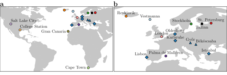
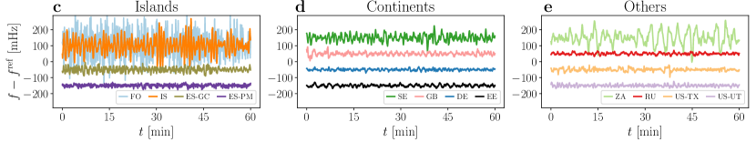
Figure 1: Overview of available frequency data. a: Different locations in Europe, Africa, and Northern America at which frequency measurements were taken. Australia and large parts of Asia or not displayed as there were no measurements recorded. b: Zoom of the European region (excluding Gran Canaria) with all locations labelled. Circles indicate measurement sites where single measurements for several days were taken, diamonds mark the four locations where we performed synchronised measurements and triangles mark sites for which we received additional data. c-e: Frequency trajectories display very different characteristics. We plot one hour extracts of the deviations from the reference frequency of $f^{\text{ref}}=50$ Hz (or $60$ Hz for the US power grids), which are offset from the zero mean to improve readability. Panels c-e and following plots abbreviate the measurement sites using the ISO 3166 code for each country and each location is assigned a colour code, as in the maps in panels a and b. For more details on the data acquisition and measurement locations see Supplementary Note 1 and Jumar2020Data . Maps were created using Python 3 and geoplots.

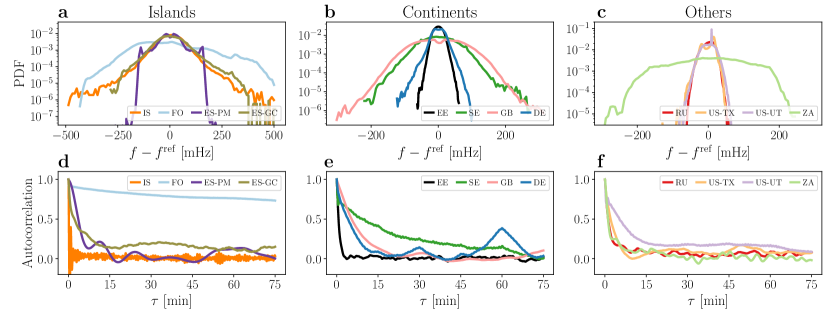
Figure 2: Heterogeneity in power grid statistics. Both histograms and autocorrelation functions display very distinct features between the different synchronous areas. a-c: Histograms of the different synchronous areas provide insight on heavy tails but also the different scales of the fluctuations. We visualise the empirical probability distributions of the various areas by histograms on a logarithmic scale. d-f: The complex autocorrelation decay reveals distinct time scales in the different grids. We compute the autocorrelation of each area for a time lag of up to 75 mins.

We recorded power grid frequency time series using a GPS synchronizsed frequency acquisition device called Electrical Data Recorder (EDR) maass2013first ; maass2015data , providing similar data as a Phasor Measurement Unit (PMU) would. Recordings were taken at local power plugs, which have been shown to give similar measurement results as monitoring the transmission grid with GPS time stamps kakimoto2006monitoring , see also Jumar2020Data for details on the data acquisition and a description of the open data base. In addition, we received a one week measurement from the Hungarian TSO for the two cities Békéscsaba and Győr. We marked the locations of the measurement locations on a geographic map in Fig. 1 a-b. Still, many more synchronous areas in the Americas, Asia, Africa, and Australia should be covered in the future.

To gain a first impression of the frequency dynamics, we visualise frequency trajectories in different synchronous areas and note quite distinct behaviour, see Fig. 1, c-e. We refer to each measurement by the country or state in which it was recorded, see also Supplementary Note 1. We group the measurements into (European) continental areas, (European) islands and other (non-European) regions, which are also mostly continental. Most islands, such as Gran Canaria (ES-GC), Faroe Islands (FO), and Iceland (IS), but also South Africa (ZA), display large deviations from the reference frequency, while the continental areas, such as the Baltic (EE) and Continental European areas (DE), as well as the measurements taken in the United States (US-UT and US-TX) and Russia (RU), stay close to the reference frequency. There are still more differences within each group: For example, the dynamics in Gran Canaria (ES-GC) and South Africa (ZA) are much more regular then the very erratic jumps of the frequency over time observable in the Faroe Islands (FO) and Iceland (IS). Finally, we do not observe any qualitative difference between $50$ and $60$ Hz areas (right), when adjusting for the different reference frequency. Note that some of the synchronous areas considered here are indeed coupled via high-voltage direct current (HVDC) lines but still possess independent synchronous behavior. Specifically, the British (GB), Continental (DE), Baltic (EE) and Nordic (SE) European areas as well as Mallorca are connected in this way. The HVDC connection of Mallorca towards Continental Europe might be the reason it displays overall smaller deviations than FO or IS, which cannot access another large synchronous area for balance.

Let us quantify the different statistics in a more systematic way by investigating distributions (histograms) and autocorrelation functions of the various areas. The distributions contain important information of how likely deviations from the reference frequency are, how large typical deviations are (width of the distribution) and whether fluctuations are Gaussian (histogram displays an inverted parabola in log-scale) and whether they are skewed (asymmetric distribution). Analysing the distributions (histograms) of the individual synchronous areas (Fig. 2 a-c), we note that the islands tend to exhibit broader and more heavy-tailed distributions than the larger continental areas. Still, there are considerable differences within each group. For example, we observe a larger standard deviation and thereby broader distribution in the Nordic (SE) and British (GB) areas compared to Continental Europe (DE), which is in agreement with earlier studies Schaefer2017a ; gorjao_data-driven_2020 . Some distributions, such as those for Russia (RU) or the Baltic grid (EE), do show approximately Gaussian characteristics while for several other areas, such as Gran Canaria (ES-GC) and Iceland (IS) they exhibit a high kurtosis ($\kappa^{\text{Iceland}}\approx 7$, as compared to $\kappa=3$ for a Gaussian), i.e., heavy tails and thereby a high probability for large frequency deviations. We provide a more detailed analysis of the first statistical moments, i.e., standard deviation $\sigma$, skewness $\beta$ and kurtosis $\kappa$ in Supplementary Note 1.

Complementary to the aggregated statistics observable in histograms, the autocorrelation function contains information on intrinsic time scales of the observed stochastic process, see Fig. 2 d-e. For simple stochastic processes such as Ornstein–Uhlenbeck processes, we would expect an exponential decay $\exp(-\gamma\tau)$ of the autocorrelation with some damping constant $\gamma$ Gardiner1985 . While most synchronous areas do show an approximately exponential decay, the decay constants vary widely. For example, the autocorrelation of the Icelandic data (IS) rapidly drops to zero, while the autocorrelation of the Nordic grid (SE) has an initial sharp drop, followed by a very slow decay. Other grids, such as the Faroe Islands (FO) or the Western interconnection (US-UT) do show a slow decay, indicating long-lasting correlations, induced e.g. via correlated noise. Finally, regular power dispatch actions every $15$ minutes are clearly observable in the Continental European (DE), British (GB) and also the Mallorcan (ES-PM) grids, consistent with earlier findings Schaefer2017a ; anvari_stochastic_2020 ; gorjao_data-driven_2020 .

Concluding, we see that histograms are a good indicator of how heavy-tailed the frequency distributions are, while the autocorrelation function reveals information on regular patterns and long term correlations. These correlations are likely connected to market activity or regulatory action, demand and generation mixture, and other aspects specific to each synchronous area. Instead of going deep into individual comparisons let us search for general applicable scaling laws instead.

Scaling of individual grids

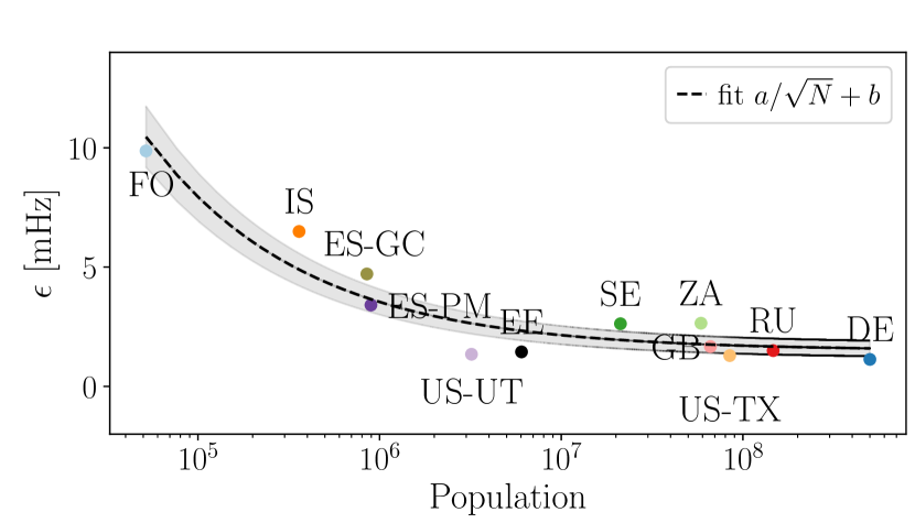
Figure 3: The noise tends to decrease with an increasing size of the synchronous area until it saturates. We plot the extracted noise amplitude $\epsilon$ compared to the logarithm of the population in a given synchronous area. The population size serves as a proxy for the total generation and consumption of that area, as data on the size of the power grids is not commonly available. The shaded area is the standard deviation of the $\epsilon$ estimation.

For the first time, we have the opportunity to analyse numerous synchronous areas of different size, ranging from Continental Europe with a yearly power generation of about $3000$ TWh ENTSOEFactsheet2018 and a population of hundreds of millions to the Faroe Islands with a population of only tens of thousands. These various areas allow us to test a previously conjectured scaling law Schaefer2017a of fluctuation amplitudes given as $\epsilon\sim 1/\sqrt{N}$, i.e., the aggregated noise amplitude $\epsilon$ in a synchronous area should decrease like the square root of the effective size of the area.

To derive this scaling relation, we formulate a Stochastic Differential Equation (SDE) of the aggregated frequency dynamics. A basic model, also known as the aggregated swing equation Machowski2011 ; Ulbig2014 , is given as

$$M\frac{\text{d}}{\text{d}t}\bar{\omega}\left(t\right)=-M\gamma\bar{\omega}\left(t\right)+\Delta P(t),$$ (1)

with bulk angular velocity $\bar{\omega}$, total inertia of a region $M$, power imbalance $\Delta P(t)$, and effective damping to inertia ratio $\gamma$, which also comprises primary control. The bulk angular velocity is the scaled deviation of the frequency from the reference: $\bar{\omega}=2\pi\!\left(f-f^{\text{ref}}\right)$ and $\Delta P(t)$ effectively represents noise acting on the system with mean $\left<\Delta P(t)\right>=0$, as generation and load are balanced on average. A simple scaling law for the frequency variability can be derived if the short-term power fluctuations at each grid node are assumed to be Gaussian. If the grid has $N$ nodes with identical noise amplitudes, the standard deviation of the power imbalance scales as

$$\sigma_{\Delta P}\sim\sqrt{N}.$$ (2)

At the same time, the total inertia typically scales linearly with the size of the grid, i.e., $M\sim N$. As a result, the amplitude of the total noise acting on the angular velocity dynamics scales as

$$\epsilon\sim\frac{1}{M}\sigma_{\Delta P}\sim\frac{1}{\sqrt{N}}.$$ (3)

A more detailed derivation is provided in Supplementary Note 2 and discussed in Schaefer2017a ; gorjao_data-driven_2020 . And a technical discussion of extracting the aggregated noise amplitude is presented in Gorjao2019 . We note that the scaling law has to be modified if the noise at the nodes is not Gaussian Schaefer2017a .

To verify the proposed scaling law in eq. (3), we approximate the number of nodes $N$ by the population of an area, since generation data are not available for all synchronous areas and population and generation tend to be approximately proportional ENTSOEFactsheet2018 . We utilise the population size as a proxy for size of the grid $N$. Indeed, we note that the aggregated noise amplitude $\epsilon$ does approximately decay with the inverse square root of the population size, as predicted, see Fig. 3. At a certain size, the noise saturates. The deviations from the prediction, such as by South Africa (ZA) and Iceland (IS) are likely caused by different local control mechanisms, or non-Gaussian noise distributions, which we focus on in the next section. Interestingly, while Faroe Islands (FO) and Mallorca (ES-PM) do display non-Gaussian probability density functions, they follow the proposed scaling law. Why this is the case and how a fully non-Gaussian scaling law could capture this even better remain open questions for future work. Still, we observe a decay of the noise, approximately following the prediction over four orders of magnitude.

Increment analysis

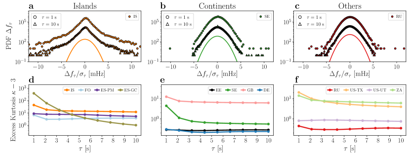
Figure 4: Increment analysis reveals non-Gaussian characteristics, dominantly in islands. Top:(a-c): We display histograms of the increments $\Delta f_{\tau}$ for the lag values $\tau=1,10$ seconds for selected areas. The curves are shifted for visibility and compared to a Gaussian distribution as reference. a: Iceland (IS) displays clear deviations from Gaussianity, even for larger increments $\tau$. b: The Nordic area (SE) displays a non-Gaussian distribution for $\tau=1\leavevmode\nobreak\ s$, but approaches a Gaussian distribution for larger delays $\tau$. c: Russia (RU) has a Gaussian increment distribution for all lags $\tau$. Bottom (d-e): We plot the excess kurtosis $\kappa-3$ for the different examined power grid frequency recordings on a log scale. We observe a non-vanishing intermittency in Gran Canaria (ES-GC), Iceland (IS), Faroe Islands (FO), Mallorca (ES-PM), Britain (GB), Texas (US-TX), and South Africa (ZA). In contrast, the increments’ distribution of the Baltic (EE), Continental Europe (DE), Nordic (SE), Russia (RU) synchronous areas, and the Western Interconnection (US-UT) approach a Gaussian distribution. See also Fig. 5 for an illustration how increments are computed from a trajectory.

In the previous section, we approximated the noise acting on each synchronous area as Gaussian to derive an approximate scaling law. In the following, we want to go beyond this simplification and investigate the rich short-time statistics present in each synchronous area. We will see in particular how non-Gaussian distributions clearly emerge on the time scale of a few seconds.

This short time scale is investigated via increments $\Delta f_{\tau}$. The increment of a frequency time series is computed as the difference of two values of the frequency with a time lag $\tau$

$$\Delta f_{\tau}=f(t+\tau)-f(t).$$ (4)

An analysis of $\Delta f_{\tau}$ provides information on how the time series changes from one time lag $\tau$ to the next. On a short time scale of $\tau\approx 1$ second the increments can be used as a proxy for the noise $\epsilon$ acting on the system, see also Supplementary Note 2.

The increments for a Wiener process, an often used reference stochastic process, are Gaussian regardless of the lag $\tau$ Gardiner1985 . However, for many real world time series, ranging from heart beats peng1993long and turbulence to solar and wind generation Anvari2016 , we observe non-Gaussian distributions for small lags $\tau$. For many such processes with non-Gaussian increments, the probability distribution functions (PDFs) of the increments tend to approach Gaussian distributions for larger increments Anvari2016 . We observe a similar behaviour for the frequency statistics, see Fig. 4. The Nordic area (SE) displays deviations from Gaussianity for small lags $\tau$ but approximates a Gaussian distribution for larger $\tau$. The Russian area (RU) even starts out with an almost Gaussian increment distributions. Contrary, the Icelandic area (IS) shows clear deviations from a Gaussian distribution for all lags $\tau$ investigated here. Still, for larger lags the pronounced tails flatten and the increment distribution slowly approaches a Gaussian distribution. The non-Gaussian increments on a short time scale point to non-Gaussian driving forces, e.g. in terms of generation or demand fluctuations acting on the power grid.

To investigate the deviations of the frequency increments from Gaussian properties, we utilise the excess kurtosis $\kappa-3$ of the distribution. Since the kurtosis $\kappa$, the normalised fourth moment of a distribution, is $\kappa^{\text{Gauss}}=3$ for a Gaussian distribution, a positive excess kurtosis points to heavy tails of the distribution.

Computing the excess kurtosis $\kappa-3$ for all our data sets, we observe variable degrees of deviation across the various synchronous areas (Fig. 4). In some areas, the intermittent behaviour of the increments $\Delta f_{\tau}$ is subdued and the overall distribution approaches a Gaussian distribution (in EE, DE, SE, RUS, and US-UT), i.e., the excess kurtosis $\kappa-3$ becomes very small ($\lesssim 10^{0}$). In contrast, all islands as well as GB, US-TX, and ZA display large and non-vanishing intermittent behaviour, with a large excess kurtosis ($\sim 10^{1}...10^{2}$). Iceland (IS), as well as Gran Canaria (ES-GC) show impressive deviations from Gaussianity, which require detailed modelling in the future.

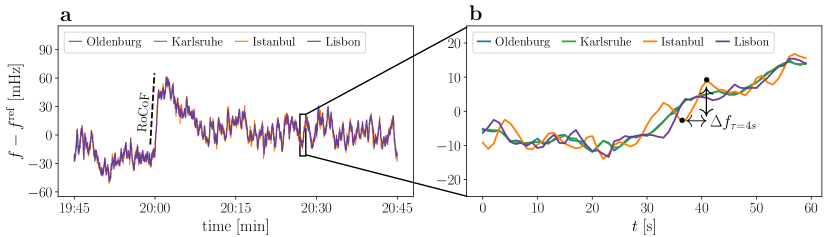
Figure 5: Synchronised measurements within the Continental European (CE) synchronous area differ on the short time scale. We show a $1$ hour frequency trajectory recorded at four different sites in the CE area: Oldenburg, Karlsruhe, Lisbon, and Istanbul. We further illustrate the RoCoF (rate of change of frequency) as the slope of the frequency every hour and the increment statistics $\Delta f_{\tau}$ as the frequency difference between two points with time lag $\tau$. For clarity, we do not include the two Hungarian measurement sites here, which produce similar results.

We summarise that smaller regions tend to display more intermittency in their increments than larger regions, again consistent with findings on the scaling of the aggregated noise amplitude $\epsilon$ (Fig. 3). Furthermore, we observe that increment distributions tend to approach Gaussian distributions for larger increments, as expected Anvari2016 , but with distinct time horizons that depend on the grid area. For most of the islands the excess kurtosis remains high even for lags of ten seconds. Contrary, in most areas of continental size the excess kurtosis is very small already for lags larger than one second. Very interesting is also the following observation: Non-Gaussian distributions in the aggregated frequency statistics (Fig. 2) are not necessarily linked with non-Gaussian increments. For example in Continental Europe (DE) we observe Gaussian increments but a non-Gaussian aggregated distribution. The deviation from Gaussianity in the aggregated distribution, e.g. in terms of frequent extreme events, is likely explained by the external drivers, such as market activities schafer2018isolating . Finally, this analysis presented here extends previous increment analyses Haehne2018 ; HaehnePropagation2019 , which only considered increments of less than a second ($\tau<1\leavevmode\nobreak\ s$), while we observe relevant non-Gaussian behaviour for larger increments ($\tau\geq 1\leavevmode\nobreak\ s$). We further analyse the differences between aggregated kurtosis and increment kurtosis in Supplementary Note 1 and discuss Castaing’s model Castaing1990 and superstatistics Beck2003 as more theoretical approaches towards increment analysis in Supplementary Note 3.

Correlated dynamics within one area

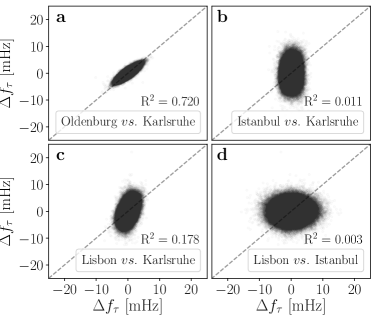
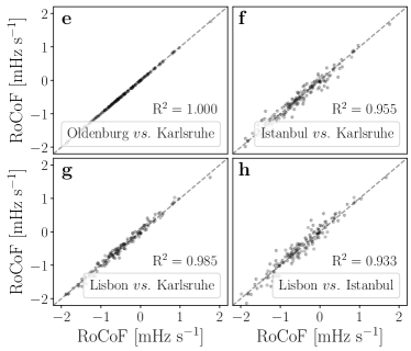
Figure 6: From localised fluctuations to bulk behaviour. From left to right, we move our focus from short time scales (increments) to long time scales (RoCoF). a-d: Short time increments are mostly independent. We compute the increment statistics $\Delta f_{\tau}=f(t+\tau)-f(t)$ for the increment time $\tau=1$​ s at the four sites in Continental Europe. The squared correlation coefficient $R^{2}$ is rounded to 4 digits. See also Supplementary Note 4 for larger lags $\tau$ and more details. e-h: Correlations at the long time scale. We record the estimated rate of change of frequency (RoCoF) $\text{d}f/\text{d}t$ every $60$ minutes for all four grid locations. In the scatter plots, each point represents the RoCoF or increment value $\Delta f_{\tau}$ computed at two different locations at the same time $t$.

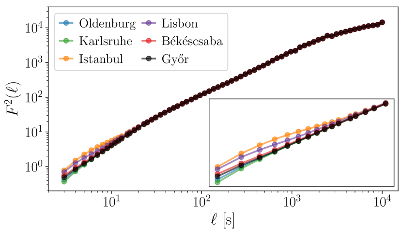
Figure 7: Detrended Fluctuation Analysis (DFA) connects short and long time scales. We perform a DFA MFDFA2020 , with order $m=1$, in accordance with Ref. meyer2020identifying , and plot the fluctuation function $F^{2}(\ell)$ as a function of the time window length $l$. The inset magnifies the values for $\ell\in\{10^{0}\dots 2\cdot 10^{1}\}$. The lines connect data points to each other to guide the eye.

Moving away from comparing individual synchronous areas, we use GPS-synchronised measurements at multiple locations within the same synchronous area, the Continental European (CE) area, marked as diamonds and triangles in Fig. 1. These measurements reveal that the frequency at different locations is almost identical on long time scales but differs on shorter time scales, see Fig. 5. While the trajectories of the two German locations, Oldenburg and Karlsruhe, are almost identical, there are visible oscillations between the frequency values recorded in Central Europe (Karlsruhe) compared to the values recorded in the peripheries (Istanbul and Lisbon).

Let us quantify this by analysing the time series at the time scale of $1$ second and hours, see Fig. 6. Increments $\Delta f_{\tau}$, as also introduced above, reveal the short-term variability of a time series. In addition, we measure the long-term correlations on a time scale of hours by determining the rate of change of frequency (RoCoF). The RoCoF is the temporal derivative of the frequency and thereby very similar to increments. However, here it has a very different meaning as we evaluate it only at every full hour and take into account several data points, see gorjao_data-driven_2020 and Methods. Thereby, the RoCoF mirrors the hourly power dispatch Weissbach2009 and gives a good indication of long-term dynamics and deterministic external forcing. In the next section, we will also investigate the intermediate time scale of several seconds and inter-area oscillations.

Short time scale dynamics, as determined by frequency increments $\Delta f_{\tau}$, are almost independent on the time scale of $\tau=1$ second, see Fig. 6 a-d. We generate scatter plots of the increment value $\Delta f_{\tau}(t)$ at the same time $t$ at two different locations. If the increments are always identical, all points should lie on a straight line with slope 1. If the increments are completely uncorrelated, we would expect a circle or an ellipse aligned with one axis. Indeed, the increments taken at the same time for Oldenburg and Karlsruhe are highly correlated and almost always identical, i.e., the points in a scatter plots follow a narrow tilted ellipse (Fig. 6 a). Moving geographically further away from Karlsruhe, the increments of Istanbul (Fig. 6 b) are completely uncorrelated with those recorded in Karlsruhe, i.e., large frequency jumps in Istanbul may take place at the same time as small jumps happen in Karlsruhe. A similar picture of uncorrelated increments emerges when comparing Lisbon and Istanbul (Fig. 6 d), while Lisbon vs. Karlsruhe displays some small correlation (Fig. 6 c). At the two peripheral locations, Lisbon and Istanbul, the increment distributions are much wider, i.e., larger jumps on a short time scale are much more common in Istanbul and Lisbon than they are in Karlsruhe. For larger lags $\tau>1\leavevmode\nobreak\ s$, the increments between all pairs become more correlated, see Supplementary Note 4.

Let us move to longer time scales. At the $60$ minute time stamps, power is dispatched in the CE grid to match the current demand, leading to a sudden surge in the frequency Weissbach2009 ; gorjao_data-driven_2020 ; anvari_stochastic_2020 . Interestingly, the frequency dynamics at the different grid sites are very similar, i.e., the deterministic event of the power dispatch is seen unambiguously everywhere in the synchronous area, almost regardless of distance, see Fig. 6. All locations closely follow the same trajectory on the $1$ hour time scale. This is reflected in highly correlated RoCoF values, with a particularly good match between Oldenburg and Karlsruhe and a linear regression coefficient of at least $R^{2}\geq 0.93$ for all pairs (Fig. 6 a-d).

We combine these different time scales in a single detrended fluctuation analysis (DFA), where we also integrate the two Hungarian locations, see Fig. 7. At short time scales, the DFA results differ for the four locations, while starting at the time scale of $t\sim 10^{1}$ seconds, the four curves coincide. For the time scale of $1$ second, all locations are subject to different fluctuations, with Istanbul and Lisbon displaying the largest values of the fluctuation function. This is coherent with results of the increment analysis, where Istanbul and Lisbon have the broadest increment distributions (Fig. 6 a-d). Moving to longer time scales of tens or hundreds of seconds, we observe a coincidence of the fluctuation function. This coincidence, i.e., identical behaviour for large time scales is in good agreement with the highly correlated RoCoF results (Fig. 6 e-h). We may also interpret this change from short term and localised dynamics to long term and bulk behaviour as a change from stochastic to deterministic dynamics, i.e., the random fluctuations are localised and take place on a short time scale, while the deterministic dispatch actions and overall trends penetrate the whole grid on a long time scale. See also Methods and Supplementary Note 5 for details on the DFA methodology.

Spatio-temporal dynamics

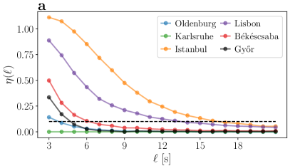
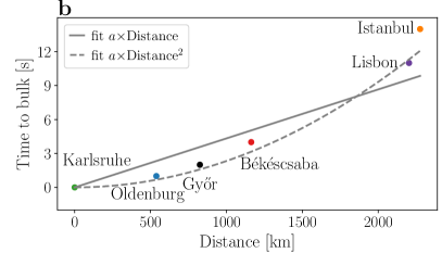
Figure 8: The time-to-bulk increases with distance. a: The relative DFA function $\eta(\ell)$ with Karlsruhe as reference; we determine the time-to-bulk as the time when this value reaches $0.1$ (dashed line), see also eq. (5). b: We plot the so extracted time-to-bulk vs. the distance from Karlsruhe and provide a simple fit for the first five points (i.e. excluding Istanbul as it clearly behaves differently). We obtain a value for the linear fit $a=5.2\times 10^{-3}$​ s​ km^-1, see Methods for details on the distance.

Next, let us investigate the spatio-temporal aspect of the synchronised measurements. We connect the transition from local fluctuations towards bulk behaviour with the geographical distance of the measurement points, complementing earlier analysis based on voltage angles cresap1981emergence ; chompoobutrgool2012identification . We determine the typical time-to-bulk, i.e., the time necessary so that the dynamics at a given node approximates the bulk behaviour. To this end, we choose Karlsruhe, Germany, as our reference, which is very central within the Continental European synchronous area. The choice of the reference does not qualitatively change the results. For each of the remaining five locations, we compute the relative DFA function

$$\eta(\ell)=\frac{{F^{2}}^{\text{location}}(\ell)-{F^{2}}^{\text{Karlsruhe}}(\ell)}{{F^{2}}^{\text{Karlsruhe}}(\ell)}$$ (5)

with respect to Karlsruhe and ask, when does this difference drop below $0.1$ (or $10\%$), i.e., when are the fluctuation at location almost indistinguishable from the ones in Karlsruhe?

The further apart two locations are, the later they reach the bulk behaviour, i.e., the larger their time-to-bulk, see Fig. 8. This observation can be intuitively understood: Two sites in close geographical vicinity are typically tightly coupled and can be synchronised by their neighbours, whereas sites far away have to stabilise on their own. Our time-to-bulk analysis quantifies this intuition. We consider both a linear and a quadratic fit. A linear dependence is expected if the bulk behaviour is realised by coupling via the shortest available path. In contrast, if the propagation is following a diffusive pattern via multiple independent paths, we would expect a quadratic dependence of the time with respect to the distance. Indeed, the quadratic fit, following diffusive coupling, is a much better fit than a linear one, as indicated by a lower Root-Mean-Squared-Error $0.5$, compared to $1.2$ seconds in the linear case. Using the newly obtained fits, we find that a location only $100$ km from Karlsruhe will have to independently stabilise fluctuations on the scale of $0.5$ to $1$ second and will then closely synchronise with the dynamics in Karlsruhe (our bulk reference). Contrary, a site $1000$ km away has to stabilise already for about $3$ to $5$ seconds before it is fully integrated in the bulk. This gives additional guidance for the control within large synchronous areas, in particular for remote and weakly coupled sites. Clearly, these first estimates demonstrate that further research is necessary to validate and adjust spatio-temporal models of the power grid zhang2019fluctuation .

Principal Component Analysis

Figure 9: Principal component analysis (PCA) of frequency recordings reveals inter-areas oscillations. a: In Continental Europe, the squared Fourier amplitudes $\left|\mathcal{F}\left(a_{m}(t)\right)\right|^{2}$ of the three dominant principal components (PCs) exhibits typical period lengths of $t\approx 7$s and $t\approx 4.5$s. b: The first spatial mode (PC1) corresponds to the bulk behaviour of the frequency and explains already $\lambda_{1}=99.2\%$ of the total variance. Contrary, the second (PC2) and third (PC3) mode reveal asynchronous inter-area modes (c-d). We refer to Supplementary Note 6 for details on the method and the results.

So far, we have focused on when and how the localised fluctuations transition into a bulk behaviour. During this transition, on the intermediate time scale of about $5$ seconds, we observe another phenomenon: ’Inter-area oscillations’, i.e., oscillations between sites in different geographical areas far apart but still within one synchronous area. Different methods are available to extract spatial inter-area modes, ranging from Empirical Mode Decomposition messina_extraction_2007 to nonlinear Koopman modes susuki_nonlinear_2011 . Here, we use a principal component analysis (PCA) bishop_pattern_2007 , which was already introduced to power systems when analysing inter-area modes and identifying coherent regions anaparthi_coherency_2005 . A PCA separates the aggregated dynamics observed in the full system into ordered principal components, which we interpret as oscillation modes. Ideally, we can explain most of the observed dynamics of the full system by interpreting a few dominant modes. Each of these modes contains information of which geographical sites are involved in the modes dynamics, similar to an eigenvector. Typical behaviour includes a translational dynamics of all sites (the eigenvector with entries 1 everywhere) or distinct oscillations between individual sites (an eigenvector with entry 1 at one site and -1 at another site).

Indeed, applying a PCA to the synchronised measurements in CE, we can capture almost the entire dynamics with just three modes, see Fig. 9. In Fig. 9 a, we provide the squared Fourier amplitudes of each mode and in Fig. 9 b-d we visualise the first three modes geographically. These three modes already explain the largest shares $\lambda_{m}$ of the total variance, see Supplementary Note 6 for the remaining modes and more details. The first mode (PC1) explains $\lambda_{1}\approx 99.2\%$ of the variance and represents the synchronous bulk behaviour of the frequency. The second (PC2) and third (PC3) mode correspond to asynchronous inter-area modes. They contribute much less to the total variance due to their small amplitude (cf. Fig. 5). In PC2 (Fig. 9 c), Western Europe forms a coherent region that is in phase opposition to Istanbul (East-West dipole), while in PC3 (Fig. 9 d), Lisbon and Istanbul swing in opposition to Oldenburg (North-South dipole). Similar results were found in an earlier theoretical study of the CE area, which also revealed global inter-area modes with dipole structures grebe_low_2010 .

The temporal dynamics of the spatial modes exhibit typical frequencies of inter-area oscillations. Fig. 9 a shows the squared Fourier amplitudes $\left|\mathcal{F}\left(a_{m}(t)\right)\right|^{2}$ of the spatial modes. The components PC2 and PC3 have their largest peaks at $t\approx 7$​ s and $t\approx 4.5$​ s, which are the periods of these inter-area modes. These periods correspond well to the typical periods of inter-area oscillations, which are reported to be $1.25$–$8$​ s Klein1991 . On larger time scales $t>12$​ s, the amplitudes $\left|\mathcal{F}\left(a_{m}(t)\right)\right|^{2}$ of the inter-area modes drop below the values of PC1. Thus, the frequency dynamics is dominated by the its bulk behaviour again, which is consistent with the estimated time-to-bulk of $12$-$15$s (Fig. 8).

Discussion

In this article, we have presented a detailed analysis of a recently published open data base of power grid frequency measurements Jumar2020Data . We have compared various independent synchronous areas, from small regions, such as the Faroe Islands and Mallorca, to large synchronous areas, like the Western Interconnection in North America and the Continental European grid, spanning areas with only tens of thousand customers to those with hundreds of millions. Especially the smaller areas tend to show a larger volatility in terms of aggregated noise but also increment intermittency, such as Iceland and Gran Canaria. We have complemented this analysis of independent grids by GPS-synchronised measurements within the Continental European power grid, revealing high correlations of the frequency at long time scales but mostly independent dynamics on fluctuation-dominated short time scales. Compared to other studies applying synchronised, wide-area measurements, such as FNET/Grideye in the US chai_wide-area_2016 or evaluations from Iceland tuttelberg2018estimation , the data we analysed here is freely available for further research Jumar2020Data .

The comparison of different synchronous areas gives us a solid foundation to test previously conjectured scaling laws of fluctuations in power grids with their size Schaefer2017a , helps us to develop synthetic models gorjao_data-driven_2020 or predict the frequency Kruse2020Predict of small grids, such as microgrids. Furthermore, aggregating standardised measurements from different areas, we can compare countries with high shares of renewables (high wind penetration in Iceland) with areas with almost no renewable generation (Mallorca) to learn how they influence the frequency dynamics and thereby the power grid stability. Similarly, this comparison also gives insights on how different market structures impact the frequency statistics and stability of a power grid.

Our results on the spatial dependencies in the Continental European (CE) synchronous area are also highly relevant for the operation of power grids and other research in the field. The observations that the long term behaviour is almost identical throughout the synchronous area but short time fluctuations differ, are in agreement with earlier theoretical findings zhang2019fluctuation . Based on the DFA results (Figs. 7 and 8), we provide a quantitative estimate that at least for the CE area already at time scales of about ten seconds, we observe an almost uniform bulk behaviour, even for locations thousands of kilometres apart. This bulk behaviour emerges much faster when locations are closer to one another.

In the regime of resonant behaviour zhang2019fluctuation , we observe inter-area oscillations with period lengths of $t=7$​ s and $t=4.5$​ s, which we extract using a principal component analysis (PCA). These time scales agree well with frequencies of inter-area oscillations reported in other studies in Europe Klein1991 ; grebe_low_2010 ; vanfretti2013spectral but also in the US cui_inter-area_2017 . However, we notice that the time scales separating bulk, resonance and local behaviour are different than the authors in a theoretical work zhang2019fluctuation assumed. There, local fluctuations were described for the $0.1$ second time scale and bulk dynamics already started at times between about $2$​ s and $5$​ s. This raises the question on how these time scales depend on the size and the dynamics of the power grid under consideration. Finally, we note that the PCA is a prime example for a model-free and data-driven analysis that still allows interpretations.

Our observation of frequency increments being independent on time scales of one second is consistent with earlier studies Haehne2018 . For Continental Europe, we find that $1$​ s-increments are correlated at small distances (below $500$ km), but independent at locations far apart. On time scales of one second and below, we cannot observe global inter-area modes anymore. Instead, we expect local fluctuations that quickly decay with distance to their origin zhang2019fluctuation ; HaehnePropagation2019 , which is consistent with our findings. The distribution of these short term fluctuation was reported to exhibit a strongly non-Gaussian distribution when subject to intermittent wind power feed-in Haehne2018 . In agreement with these results, the non-Gaussian effects vanish on time scales above one second in our recordings from Continental Europe. However, in other, particularly smaller, synchronous areas we even observe heavy-tailed increment distributions on times scales up to $10$​ s. This is likely related to the grid size and control regulations, although a detailed explanation still remains open.

In this paper, we connect the mathematics and physics communities with the engineering community, by providing potent data analysis tools from the theoretical side and then connecting these findings in the practical domain of power grid dynamics without the use of an explicit model. Both the data analysis and its interpretation could be very useful for the operation of individual grids. Our insights for the scaling could be used to improve control mechanisms, such as demand side management tchuisseu2017 , while our spreading insights give further indications about how fast cascading failures will spread throughout the power grid schafer2019dynamical . Several grid operators as well as other researchers have likely recorded power grid frequency time series at many more grid locations than we could provide in this single study. All such recordings from different sources should be combined to enable more comparisons between the dynamics of synchronous areas of different sizes and under different conditions. The data base studied here Jumar2020Data may offer a valuable starting point for such endeavours.

Because data are still only scarcely available, there remain many open questions: Can we systematically determine a propagation velocity of disturbances through the grid and compare these with theoretical predictions pagnier2019inertia ; zhang2019fluctuation ; schroeder2019dynamic ? Can we identify other time series influencing the power grid frequency dynamics and quantify their correlation such as hydro power plants in the Nordic area or demand of aluminium plants in Iceland? Can we extract the impact of market activities on the frequency dynamics in all synchronous areas? From a statistical modelling perspective, it would be interesting to investigate the scaling of higher moments, i.e. skewness and kurtosis, with time lag and size in more detail. These questions constitute only a small selection from a multitude that an open data base may help to address from a broad, interdisciplinary perspective, including engineering, mathematics, data science, time series analysis, and many other fields.

Methods

Data selection

We make use of the open data base, described in detail in Jumar2020Data to perform all analysis presented in the main text and in Supplementary Notes 1 to 6. This data set contains recordings of twelve independent synchronous regions recorded between 2017 and 2020. While some locations, such as the Faroe Islands only contain a single week of data, other regions, such as Continental Europe have been monitored for several months or years, for more details see Jumar2020Data . However, due to some technical difficulties, e.g. loss of GPS signal or unplugging the device, some measurements are not a number, i.e., "NaN" and are tagged as not reliable in the data base. These entries have been deleted to compute the histograms and statistical measures in Supplementary Note 1. To compute the autocorrelation function, as well as for the analysis of the synchronised measurement in Continental Europe, we selected the longest possible trajectory without any "NaN" entries. As a final note: From the available Gran Canaria data, we are using the March 2018 data.

RoCoF computation

When determining the rate of change of frequency (RoCoF), i.e., the time derivative of the frequency, we follow the same procedure as has been outlined in gorjao_data-driven_2020 : We select a short time window centred around the anticipated dispatch jumps at $60$ minutes of about $25$ seconds length, i.e. starting at (X):59:48 and lasting until (X+1):00:12 for all hours X. Then, we fit this short frequency trajectory with a linear function $f(t)=a+bt$. We are not interested in the offset $a$ but the value of $b$ gives us the slope of the frequency changes, i.e., the time derivative of the frequency is approximately given as $\frac{\text{d}f}{\text{d}t}\approx b$.

Detrended Fluctuation Analysis (DFA)

To carry out the detrended fluctuation analysis (DFA), we follow a similar procedure as outlined in meyer2020identifying , using the package outlined in ref. MFDFA2020 . The main idea is to detrend the data and extract the most dominant time scales by measuring the scaling behaviour of the data from increasing segments of data. The commonly denoted fluctuation function $F^{2}(\ell)$, function of the segment size $\ell$ on the time series, accounts for the variance of segmented data of increasing size. The scaling of the underlying process or processes can thus be extracted. In meyer2020identifying a detailed study of the different time scales in power grid frequencies can be found, largely focusing on scales of about ten seconds and above, whereas we put particular emphasis on the smallest time scales available, of the order of $1$ second. More details are given in Supplementary Note 5.

Time-to-bulk

To extract the time-to-bulk, seen in Fig. 8, we take the measurements of the Detrended Fluctuation Analysis (DFA) in Fig. 7 and utilise Karlsruhe as the reference for comparison. Having Karlsruhe as a reference, we compare the normalised fluctuations $\eta(\ell)$:

$$\eta(\ell)=\frac{{F^{2}}^{\text{location}}(\ell)-{F^{2}}^{\text{Karlsruhe}}(\ell)}{{F^{2}}^{\text{Karlsruhe}}(\ell)},$$ (6)

(eq. (5) in the main text), to extract the excess fluctuation at the different locations. As there is no standard, we choose a threshold value of $10\%$ for fluctuations at the different recordings to be identical. Once $\eta(\ell)$ drops below this threshold of $10\%$, the datasets are considered to be identical. In this manner, we determine the time-to-bulk as the necessary time of a recording to exhibit the same fluctuation behaviour as the reference of Karlsruhe. The distance measures taken are the geographic distances with respect to Karlsruhe, applying OpenStreet Maps https://www.openstreetmap.org/ and using the routing by Foot(OSRM). This yields the following distances from Karlsruhe: Oldenburg: $538$​ km, Győr: $825$​ km, Békéscsaba: $1163$​ km, Lisbon: $2203$​ km, Istanbul: $2276$​ km. The reason to use route finding by foot is that the power grid is not taking any air plane routes but is limited also to the shortest routes available in the transmission grid. These distances in the power system might be even longer where transmission line density is low. Note that our choice of geographical distance does not apply any assumption on the underlying power grid topology. With fully (yet currently unavailable) information about all operational transmission lines, a shortest path distance on the transmission network would be an alternative HaehnePropagation2019 .

Data availability

Frequency recordings are described in detail in Jumar2020Data . An open repository containing all recordings can be accessed here: https://osf.io/by5hu/. The Hungarian TSO data is available here: https://osf.io/m43tg/. All data that support the results presented in the figures of this study are available from the authors upon reasonable request.

Code availability

Code to produce the presented analysis and figures is available on github: https://github.com/LRydin

Author contributions

L.R.G., R.J., H.M., V.H., G.C.Y., J.K., M.T., C.B., D.W., and B.S. conceived and designed the research. R.J. and H.M. constructed the measurement device and evaluated the experimental data. L.R.G., J.K., and B.S. performed the data analysis and generated the figures. All authors contributed to discussing and interpreting the results and writing the manuscript.

Competing interests

The Authors declare no Competing Financial or Non-Financial Interests.

References

- (1) Sawin, J. L. et al. Renewables 2018–Global status report (2018).
- (2) Meadowcroft, J. What about the politics? Sustainable development, transition management, and long term energy transitions. Policy Sciences 42, 323 (2009).
- (3) Markard, J. The next phase of the energy transition and its implications for research and policy. Nature Energy 3, 628–633 (2018).
- (4) Rodríguez-Molina, J., Martínez-Núñez, M., Martínez, J.-F. & Pérez-Aguiar, W. Business models in the smart grid: Challenges, opportunities and proposals for prosumer profitability. Energies 7, 6142–6171 (2014).
- (5) Fang, X., Misra, S., Xue, G. & Yang, D. Smart Grids - The new and improved Power Grid: A Survey. Communications Surveys & Tutorials, IEEE 14, 944–980 (2012).
- (6) Bärwaldt, G. Energy revolution needs interpreters. ATZelektronik worldwide 13, 68–68 (2018).
- (7) Parag, Y. & Sovacool, B. K. Electricity market design for the prosumer era. Nature Energy 1, 16032 (2016).
- (8) Kundur, P., Balu, N. J. & Lauby, M. G. Power system stability and control, vol. 7 (McGraw-Hill, New York, 1994).
- (9) Anvari, M. et al. Short term fluctuations of wind and solar power systems. New Journal of Physics 18, 063027 (2016).
- (10) Wolff, M. F. et al. Heterogeneities in electricity grids strongly enhance non-Gaussian features of frequency fluctuations under stochastic power input. Chaos: An Interdisciplinary Journal of Nonlinear Science 29, 103149 (2019).
- (11) Wohland, J., Omrani, N. E., Keenlyside, N. & Witthaut, D. Significant multidecadal variability in German wind energy generation. Wind Energy Science 4, 515–526 (2019).
- (12) Hartmann, B., Vokony, I. & Táczi, I. Effects of decreasing synchronous inertia on power system dynamics–Overview of recent experiences and marketisation of services. International Transactions on Electrical Energy Systems 29, e12128 (2019).
- (13) Filatrella, G., Nielsen, A. H. & Pedersen, N. F. Analysis of a Power Grid using a Kuramoto-like Model. The European Physical Journal B 61, 485–491 (2008).
- (14) Schmietendorf, K., Peinke, J., Friedrich, R. & Kamps, O. Self-organized synchronization and voltage stability in networks of synchronous machines. The European Physical Journal Special Topics 223, 2577–2592 (2014).
- (15) Nishikawa, T. & Motter, A. E. Comparative analysis of existing models for power-grid synchronization. New Journal of Physics 17, 015012 (2015).
- (16) Rohden, M., Sorge, A., Timme, M. & Witthaut, D. Self-organized Synchronization in Decentralized Power Grids. Physical Review Letters 109, 064101 (2012).
- (17) Menck, P. J., Heitzig, J., Marwan, N. & Kurths, J. How Basin Stability Complements the Linear-stability Paradigm. Nature Physics 9, 89–92 (2013).
- (18) Rodrigues, F. A., Peron, T. K. D., Ji, P. & Kurths, J. The Kuramoto model in complex networks. Physics Reports 610, 1–98 (2016).
- (19) Schäfer, B. et al. Escape routes, weak links, and desynchronization in fluctuation-driven networks. Physical Review E 95, 060203 (2017).
- (20) Hindes, J., Jacquod, P. & Schwartz, I. B. Network desynchronization by non-Gaussian fluctuations. Physical Review E 100, 052314 (2019).
- (21) Zhang, X., Hallerberg, S., Matthiae, M., Witthaut, D. & Timme, M. Fluctuation-induced distributed resonances in oscillatory networks. Science Advances 5, eaav1027 (2019).
- (22) Hähne, H., Schmietendorf, K., Tamrakar, S., Peinke, J. & Kettemann, S. Propagation of wind-power-induced fluctuations in power grids. Physical Review E 99, 050301 (2019).
- (23) Schäfer, B., Matthiae, M., Timme, M. & Witthaut, D. Decentral Smart Grid Control. New Journal of Physics 17, 015002 (2015).
- (24) Poolla, B. K., Bolognani, S. & Dörfler, F. Optimal placement of virtual inertia in power grids. IEEE Transactions on Automatic Control 62, 6209–6220 (2017).
- (25) Pagnier, L. & Jacquod, P. Inertia location and slow network modes determine disturbance propagation in large-scale power grids. PLOS ONE 14, e0213550 (2019).
- (26) Simonsen, I., Buzna, L., Peters, K., Bornholdt, S. & Helbing, D. Transient dynamics increasing network vulnerability to cascading failures. Physical Review Letters 100, 218701 (2008).
- (27) Yang, Y., Nishikawa, T. & Motter, A. E. Small vulnerable sets determine large network cascades in power grids. Science 358, eaan3184 (2017).
- (28) Schäfer, B. & Yalcin, G. C. Dynamical modeling of cascading failures in the Turkish power grid. Chaos: An Interdisciplinary Journal of Nonlinear Science 29, 093134 (2019).
- (29) Nesti, T., Zocca, A. & Zwart, B. Emergent failures and cascades in power grids: a statistical physics perspective. Physical Review Letters 120, 258301 (2018).
- (30) Chai, J. et al. Wide-area measurement data analytics using FNET/GridEye: A review. In 2016 Power Systems Computation Conference (PSCC) (2016).
- (31) MagnaGen GmbH. Gridradar–an independent grid monitoring system. https://gridradar.net/ (2020).
- (32) Lasseter, R. H. & Paigi, P. Microgrid: A conceptual solution. In 2004 IEEE 35th Annual Power Electronics Specialists Conference (PESC), vol. 6, 4285–4290 (IEEE, 2004).
- (33) Jumar, R., Maaß, H., Schäfer, B., Gorjão, L. R. & Hagenmeyer, V. Power grid frequency data base. arXiv preprint arXiv:2006.01771 (2020).
- (34) Maaß, H. et al. First evaluation results using the new electrical data recorder for power grid analysis. IEEE Transactions on Instrumentation and Measurement 62, 2384–2390 (2013).
- (35) Maaß, H. et al. Data processing of high-rate low-voltage distribution grid recordings for smart grid monitoring and analysis. EURASIP Journal on Advances in Signal Processing 2015, 14 (2015).
- (36) Jumar, R., Maaß, H., Schäfer, B., Gorjão, L. R. & Hagenmeyer, V. Power grid frequency data base. https://osf.io/by5hu/ (2020).
- (37) Kakimoto, N., Sugumi, M., Makino, T. & Tomiyama, K. Monitoring of interarea oscillation mode by synchronized phasor measurement. IEEE Transactions on Power Systems 21, 260–268 (2006).
- (38) Schäfer, B., Beck, C., Aihara, K., Witthaut, D. & Timme, M. Non-Gaussian power grid frequency fluctuations characterized by Lévy-stable laws and superstatistics. Nature Energy 3, 119–126 (2018).
- (39) Rydin Gorjão, L. et al. Data-driven model of the power-grid frequency dynamics. IEEE Access 8, 43082–43097 (2020).
- (40) Gardiner, C. W. Handbook of Stochastic Methods: for Physics, Chemistry and the Natural Sciences (Springer, 1985).
- (41) Anvari, M. et al. Stochastic properties of the frequency dynamics in real and synthetic power grids. Physical Review Research 2, 013339 (2020).
- (42) ENTSO-E. Statistical factsheet 2018. https://docstore.entsoe.eu/Documents/Publications/Statistics/Factsheet/entsoe_sfs2018_web.pdf (2018).
- (43) Machowski, J., Bialek, J. & Bumby, J. Power System Dynamics: Stability and Control (John Wiley & Sons, Chichester, 2011).
- (44) Ulbig, A., Borsche, T. S. & Andersson, G. Impact of low rotational inertia on power system stability and operation. IFAC Proceedings Volumes 47, 7290–7297 (2014).
- (45) Rydin Gorjão, L. & Meirinhos, F. kramersmoyal: Kramers–Moyal coefficients for stochastic processes. Journal of Open Source Software 4, 1693 (2019).
- (46) Peng, C.-K. et al. Long-range anticorrelations and non-Gaussian behavior of the heartbeat. Physical Review Letters 70, 1343 (1993).
- (47) Schäfer, B., Timme, M. & Witthaut, D. Isolating the impact of trading on grid frequency fluctuations. In 2018 IEEE PES Innovative Smart Grid Technologies Conference Europe (ISGT-Europe), 1–5 (IEEE, 2018).
- (48) Hähne, H., Schottler, J., Wächter, M., Peinke, J. & Kamps, O. The footprint of atmospheric turbulence in power grid frequency measurements. Europhysics Letters 121, 30001 (2018).
- (49) Castaing, B., Gagne, Y. & Hopfinger, E. Velocity probability density functions of high Reynolds number turbulence. Physica D: Nonlinear Phenomena 46, 177–200 (1990).
- (50) Beck, C. & Cohen, E. G. D. Superstatistics. Physica A 322, 267–275 (2003).
- (51) Rydin Gorjão, L. MFDFA: Multifractal Detrended Fluctuation Analysis in Python. https://zenodo.org/record/3625759 (2020).
- (52) Meyer, P. G., Anvari, M. & Kantz, H. Identifying characteristic time scales in power grid frequency fluctuations with dfa. Chaos: An Interdisciplinary Journal of Nonlinear Science 30, 013130 (2020).
- (53) Weißbach, T. & Welfonder, E. High Frequency Deviations within the European Power System–Origins and Proposals for Improvement. VGB powertech 89, 26 (2009).
- (54) Cresap, R. & Hauer, J. Emergence of a new swing mode in the western power system. IEEE Transactions on Power Apparatus and Systems 2037–2045 (1981).
- (55) Chompoobutrgool, Y. & Vanfretti, L. Identification of power system dominant inter-area oscillation paths. IEEE Transactions on Power Systems 28, 2798–2807 (2012).
- (56) Messina, A. R. & Vittal, V. Extraction of dynamic patterns from wide-area measurements using empirical orthogonal functions. IEEE Transactions on Power Systems 22, 682–692 (2007).
- (57) Susuki, Y. & Mezic, I. Nonlinear Koopman modes and coherency identification of coupled swing dynamics. IEEE Transactions on Power Systems 26, 1894–1904 (2011).
- (58) Bishop, C. M. Pattern Recognition and Machine Learning (Springer, New York, 2007), 1 edn.
- (59) Anaparthi, K., Chaudhuri, B., Thornhill, N. & Pal, B. Coherency identification in power systems through principal component analysis. IEEE Transactions on Power Systems 20, 1658–1660 (2005).
- (60) Grebe, E., Kabouris, J., Lopez Barba, S., Sattinger, W. & Winter, W. Low frequency oscillations in the interconnected system of Continental Europe. In IEEE PES General Meeting, 1–7 (IEEE, Minneapolis, MN, 2010).
- (61) Klein, M., Rogers, G. J. & Kundur, P. A fundamental study of inter-area oscillations in power systems. IEEE Transactions on Power Systems 6, 914–921 (1991).
- (62) Tuttelberg, K., Kilter, J., Wilson, D. & Uhlen, K. Estimation of power system inertia from ambient wide area measurements. IEEE Transactions on Power Systems 33, 7249–7257 (2018).
- (63) Kruse, J., Schäfer, B. & Witthaut, D. Predicting the power grid frequency. arXiv preprint arXiv:2004.09259 (2020).
- (64) Vanfretti, L., Bengtsson, S., Perić, V. S. & Gjerde, J. O. Spectral estimation of low-frequency oscillations in the Nordic grid using ambient synchrophasor data under the presence of forced oscillations. In 2013 IEEE Grenoble Conference, 1–6 (IEEE, 2013).
- (65) Cui, Y. et al. Inter-area oscillation statistical analysis of the U.S. Eastern interconnection. The Journal of Engineering 2017, 595–605 (2017).
- (66) Tchuisseu, E. T., Gomila, D., Brunner, D. & Colet, P. Effects of dynamic-demand-control appliances on the power grid frequency. Physical Review E 96, 022302 (2017).
- (67) Schröder, M., Zhang, X., Wolter, J. & Timme, M. Dynamic perturbation spreading in networks. IEEE Transactions on Network Science and Engineering (2019).