Least $\bm{k}$th-Order and Rényi Generative Adversarial Networks

Abstract

We investigate the use of parametrized families of information-theoretic measures to generalize the loss functions of generative adversarial networks (GANs) with the objective of improving performance. A new generator loss function, called least $k$th-order GAN (L$k$GAN), is first introduced, generalizing the least squares GANs (LSGANs) by using a $k$th order absolute error distortion measure with $k\geq 1$ (which recovers the LSGAN loss function when $k=2$). It is shown that minimizing this generalized loss function under an (unconstrained) optimal discriminator is equivalent to minimizing the $k$th-order Pearson-Vajda divergence. Another novel GAN generator loss function is next proposed in terms of Rényi cross-entropy functionals with order $\alpha>0$, $\alpha\neq 1$. It is demonstrated that this Rényi-centric generalized loss function, which provably reduces to the original GAN loss function as $\alpha\to 1$, preserves the equilibrium point satisfied by the original GAN based on the Jensen-Rényi divergence, a natural extension of the Jensen-Shannon divergence.

Experimental results indicate that the proposed loss functions, applied to the MNIST and CelebA datasets, under both DCGAN and StyleGAN architectures, confer performance benefits by virtue of the extra degrees of freedom provided by the parameters $k$ and $\alpha$, respectively. More specifically, experiments show improvements with regard to the quality of the generated images as measured by the Fréchet Inception Distance (FID) score and training stability. While it was applied to GANs in this study, the proposed approach is generic and can be used in other applications of information theory to deep learning, e.g., the issues of fairness or privacy in artificial intelligence.

Deep learning, generative adversarial networks, Rényi cross-entropy, Jensen-Rényi divergence, Pearson-Vajda divergence.

1 Introduction

Generative models have garnered significant attention in recent years. The main approaches for such models include generative adversarial networks (GANs) [21], [6], [49], [14], autoencoders/variational autoencoders (e.g. VAEs) [28], generative autoregressive models [44], invertible flow based latent vector models [29], and hybrids of the above models [22]. Compared to other approaches, GANs have generated the most interest (e.g., see surveys in [14], [57], [58]). Generative models are used in reinforcement learning, time series predictions, fairness and privacy in artificial intelligence (AI) [9], disentanglement [46], and can also be trained in a semi-supervised manner, where labels and training examples are missing. Furthermore, these models are designed to produce several different outputs that are equally acceptable [20], [27].

Approximation methods are needed in the case of VAEs and furthermore, the approximate probability distribution is not guaranteed to converge to the true distribution [37], [38], [6]. In contrast, GANs optimize a loss function which is constructed using ideas from game and information theory. Notably, GANs can represent distributions that lie on low dimensional manifolds, which VAEs and estimating densities are unable to do [6]. Moreover, GANs do not rely on Markov chains and variational bounds are not necessarily needed [20].

1.1 Prior work

The original GANs [21] consist of a generative neural network competing with a discriminative neural network in a min-max game. Several variants of GANs have been studied and implemented. Deep convolutional GANs (DCGANs) use convolutional layers to learn higher dimensional dependencies that are inherent in complex datasets such as images [49]. Although DCGANs produced better results than other state-of-the-art generative models such as VAEs and autoregressive models, they can be difficult to train and can suffer from mode collapse [6, 58]. Mode collapse occurs when the generator produces outputs that significantly lack in diversity (i.e. producing mostly one output with little variations), while the discriminator is able to tell apart real from fake data perfectly during training. Researchers have diligently attempted to fix the aforementioned issues. For example, StyleGANs [27] change the architecture of the generative neural network to produce realistic high resolution images, while Wasserstein GANs [6] address the problem of mode collapse by using the Wasserstein-1 distance as the loss function.

GANs have been applied to data privacy problems, where the goal is to hide certain features of user data to protect their privacy, but mask these features judiciously in order not to compromise other useful data [26]. Related problems of AI fairness can be addressed using this strategy. GANs have also been widely used for computer vision problems, such as generating fake images of handwritten numbers, or landscape paintings [20]. Thus the flexibility of GAN design allows for innovation and applicability to a wide range of data and use cases.

The use of information theory to study and improve neural networks is a relatively new yet promising direction of research; e.g., see [32, 43, 47, 2, 12, 59, 53, 4, 61, 60] and the references therein. While many GANs loss functions are based on the Jensen-Shannon divergence, there are other divergence measures and tools in information theory that can be directly applied to the design of GANs. The family of loss functions that simplify down to $f$-divergences was thoroughly studied in [43, 19], and [33]. Bridging the gap between maximum likelihood learning and GANs, especially those with loss functions that simplify down to $f$-divergences, has also been analyzed in [61]. Using the symmetric Kullback-Leibler (KL) divergence, researchers have also shown that a variant of VAEs is connected to GANs [11]. InfoGANs use variational mutual information maximization with latent codes to achieve unsupervised representation learning with considerable success [12].

A new least squares loss function that simplifies down to the Pearson $\chi^{2}$ divergence was examined in [37]. Through experiments, it was illustrated that the resulting least squares GANs (LSGANs) are more stable than DCGANs. The promising results of LSGANs and the fact that the Pearson-Vajda $|\chi|^{k}$ divergence of order $k\geq 1$ generalizes the Pearson $\chi^{2}$ divergence is one motivation for this study.

The use of the Rényi divergence in the context of GANs is a recent development. Rényi used the simplest set of postulates that characterize Shannon’s entropy and introduced his own entropy and divergence measures (parametrized by its order $\alpha$) that generalize the Shannon entropy and the KL divergence, respectively [50]. Moreover, the original Jensen-Rényi divergence [24] as well as the identically named divergence [30] used in this paper are non-$f$-divergence generalizations of the Jensen-Shannon divergence. Traditionally, Rényi’s entropy and divergence have had applications in a wide range of problems, including lossless data compression [10, 13, 48], hypothesis testing [16, 3], error probability [7], and guessing [5, 56]. Recently, the Rényi divergence and its variants (including Sibson’s mutual information) were used to bound the generalization error in learning algorithms [18], and to analyze deep neural networks (DNNs) [59], variational inference [35], Bayesian neural networks [34], and generalized learning vector quantization [40]. Furthermore Cumulant GANs proposed a new loss function using the cumulant generating function, which subsumes the Rényi, KL, and reverse KL divergences as special cases, and is experimentally shown to be more robust than Wasserstein GANs [45]. Hence, generalizing the GANs loss function using Rényi divergence provides another motivation for this work.

1.2 Contributions

The novel contributions of this work are described in what follows. We revisit the LSGAN and original GAN generator loss functions by considering more general parametrized classes of loss functions that subsume the original loss functions as a special case. An important objective is to identify generalized loss functions that can be analytically minimized under an (unconstrained) optimal discriminator, with the minimum theoretically achieved when the generator’s distribution is the true dataset distribution.

More specifically, we first introduce least $k$th-order GANs (L$k$GANs) by using the $k$th-order absolute error loss function for the generator ($k\geq 1$). We prove that minimizing this loss function is equivalent to minimizing the $k$th-order Pearson-Vajda divergence [42], which recovers the Pearson $\chi^{2}$ divergence examined in [37] when $k=2$. The L$k$GANs’ generator loss function also preserves the theoretical minimum of LSGANs’ generator loss function, which is achieved when the generator’s distribution is equal to the true distribution. L$k$GANs are implemented and compared with LSGANs on the CelebA [36] dataset using the StyleGAN architecture. Experimentally, L$k$GANs are shown to outperform LSGANs in terms of generated image quality, as measured by the Fréchet inception distance (FID) score [25], and the rate at which they converge to meaningful results. L$k$GANs are also observed to reduce the problem of mode collapse during training.

We also revisit the original GAN’s generator optimization problem via the novel use of Rényi information measures of order $\alpha$ (with $\alpha>0$ and $\alpha\neq 1$). To this end, we consider the Jensen-Rényi divergence as well as the differential Rényi cross-entropy, which is the continuous form of the Rényi cross-entropy studied in [54]. We show that the differential Rényi cross-entropy generalizes the Shannon differential cross-entropy and prove that it is monotonically decreasing in $\alpha$. With these Rényi measures in place, we propose a new GAN’s generator loss function expressed in terms of the negative sum of two Rényi cross-entropy functionals. We show that minimizing this $\alpha$-parametrized loss function under an optimal discriminator results in the minimization of the Jensen-Rényi divergence [30], which is a natural extension of the Jensen-Shannon divergence as it uses the Rényi divergence instead of the Kullback-Leibler (KL) divergence in its expression. We also prove that our generator loss function of order $\alpha$ converges to the original GAN loss function in [21] when $\alpha\to 1$. Previously, the GANs loss function has been generalized using the $f$-divergence measure [15, 43]. However, as the Jensen-Rényi divergence is not itself an $f$-divergence, it can be interpreted as a non-$f$-divergence generalization of the Jensen-Shannon divergence. We call the resulting GAN network RényiGAN.

In a concurrent work [51], a Rényi-based GAN is developed, called RGAN, by also using a “Rényi cross-entropy” to generalize the original GAN loss function and it is shown that the resulting loss function is stable in terms of its absolute condition number (calculated using functional derivatives). Note that RényiGAN is based on a different Rényi cross-entropy definition from the one used in RGAN [51]. Hence, unlike what it is claimed in [51] by referencing the preprint [8] of this paper, the RGAN’s loss function does not generalize the RényiGAN loss functions presented herein. Moreover unlike RényiGAN, the RGAN loss function does not preserve the GANs theoretical result that the optimal generator for an optimal discriminator induces a probability distribution equal to the true dataset distribution. Using a similar stability analysis to the one carried out for RGANs in [51], we derive the absolute condition number of our Rényi cross-entropy measure and show that the RényiGAN’s generator loss function is stable for $\alpha\geq 2$. This result complements the one derived in [51], where stability of the RGAN loss function is shown for sufficiently small values of $\alpha$.

Finally, we implement the newly proposed RényiGAN loss function using the DCGAN and StyleGAN architectures [27]. Our experiments use the MNIST [31] and CelebA [36] datasets and provide comparisons with the baseline DCGAN and StyleGAN systems. Experiments show that the Rényi-centric GAN systems perform as well as, or better, than their baseline counterparts in terms of visual quality of the generated images (as measured by the FID score), particularly when spanning $\alpha$ over a range of values as it helps the avoidance of local minimums. We show that employing $L_{1}$ normalization with the Rényi generator loss function confers greater stability, quicker convergence, and better FID scores for both RényiGANs and DCGANs. Consistent stability and slightly improved FID scores are also noted when comparing RényiStyleGAN with StyleGAN. We finally compare these GAN systems with the simplified gradient penalty [39], showing that the Rényi-type systems provide substantial reductions in computational training time vis-a-vis the baselines, for similar levels of FID.

The rest of the paper is organized as follows. In Section 2, we present the definitions of divergence measures and introduce a natural extension of the (differential) Shannon cross-entropy, the (differential) Rényi cross-entropy. In Section 3, we analyze L$k$GANs, which generalize LSGANs, and provide experimental results. In Section 4, we present theoretical results of RényiGANs, which generalize GANs, and show experimental results comparing RényiGANs with DCGANs and StyleGANs. Finally, we provide conclusions in Section 5.

2 Divergence Measures

Divergence measures are used to quantify the dissimilarity between distributions. We recall the definitions of the Kullback-Leibler divergence, the (differential) Shannon cross-entropy, and the Pearson-Vajda and Rényi divergences. We also present the definition of the (differential) Rényi cross-entropy and examine some of its properties. We also present the Jensen-Rényi divergence, which is a natural extension of the Jensen-Shannon divergence by virtue of being a mixture of two Rényi divergences. This Jensen-Rényi divergence was recently introduced in [30] for discrete distributions and studied in the context of generalized (Rényi-type) $f$-divergences. It differs from the identically named divergence studied in [24] and [23], an earlier extension of the Jensen-Shannon divergence consisting of the difference between the Rényi entropy of a mixture of multiple probability distributions and the mixture of the Rényi entropies of the individual distributions. Other recent (but different) extensions of the Jensen-Shannon divergence can be found in [41] and the references therein.

Let $p$ and $q$ be two probability densities with common support $\mathcal{R}\subset$ on the Lebesgue measurable space $(,\mathcal{B}(),\mu)$, and let

$$\mathrm{KL}(p\|q):=\int_{\mathcal{R}}p\log\frac{p}{q}\,\mathrm{d}\mu\qquad\text{and}\qquad h(p;q):=-\int_{\mathcal{R}}p\log q\,\mathrm{d}\mu$$ (1)

denote the KL divergence and the differential Shannon cross-entropy between $p$ and $q$, respectively, where both information measures are assumed to be finite. In (1) and throughout, we use the short form $\int_{\mathcal{R}}f\,\mathrm{d}\mu:=\int_{x\in\mathcal{R}}f(x)\,\mathrm{d}\mu(x)$ for any measurable function $f$. When $p=q$ almost everywhere (a.e.), then $h(p;q)$ reduces to the differential Shannon entropy of $p$, denoted by $h(p)$. We next describe the Pearson-Vajda divergence, which is itself an $f$-divergence [42].

Definition 1.

The Pearson-Vajda divergence of order $\bm{k}$, $|\chi|^{k}(p\|q)$, between $p$ and $q$, where $k\geq 1$, is given by

$$|\chi|^{k}(p\|q):=\int_{\mathcal{R}}\frac{|q-p|^{k}}{p^{k-1}}\mathrm{d}\mu.$$ (2)

Note that $|\chi|^{k}(p\|q)\geq 0$ with equality if and only if (iff) $p=q$ (a.e.). Also when $k=2$, $|\chi|^{k}(\cdot\|\cdot)$ reduces to the Pearson $\bm{\chi^{2}}$ divergence:

$$\chi^{2}(p\|q):=\int_{\mathcal{R}}\frac{(q-p)^{2}}{p}\mathrm{d}\mu.$$ (3)

Definition 2.

The Rényi divergence of order $\bm{\alpha}$ between $p$ and $q$, where $\alpha>0$, $\alpha\neq 1$, is given by

$$\mathrm{D}_{\alpha}(p\|q):=\frac{1}{\alpha-1}\log\left(\int_{\mathcal{R}}p^{\alpha}q^{1-\alpha}\mathrm{d}\mu\right).$$ (4)

Note that $\mathrm{D}_{\alpha}(p\|q)\geq 0$ with equality iff $p=q$ (a.e.). Furthermore, if $\mathrm{D}_{\gamma}(p\|q)<\infty$ for some $\gamma>1$, then, as shown in [55], we have that

$$\lim_{\alpha\rightarrow 1}\mathrm{D}_{\alpha}(p\|q) = \mathrm{KL}(p\|q).$$ (5)

For simplicity of analysis, we assume in what follows the finiteness of $\mathrm{D}_{\gamma}(\cdot\|\cdot)$ for some $\gamma>1$ so that convergence of (5) holds. Being a function of an $f$-divergence, useful properties and bounds on the Rényi divergence can be elucidated from the study of $f$-divergences, see [52] and related references.

Definition 3.

The differential Rényi cross-entropy of order $\bm{\alpha}$ between $p$ and $q$, where $\alpha>0$, $\alpha\neq 1$, is given by

$$h_{\alpha}(p;q) := \frac{1}{1-\alpha}\log\left(\int_{\mathcal{R}}pq^{\alpha-1}\mathrm{d}\mu\right).$$ (6)

When $p=q$ (a.e.), $h_{\alpha}(p;q)$ reduces to the Rényi entropy, $h_{\alpha}(p):=\frac{1}{1-\alpha}\log\left(\int_{\mathcal{R}}p^{\alpha}\mathrm{d}\mu\right)$. We next show that $\lim_{\alpha\rightarrow 1}h_{\alpha}(p;q)=h(p;q)$ under some finiteness conditions.

Theorem 1.

If $h(p;q)<\infty$, then

$$\lim_{\alpha\downarrow 1}h_{\alpha}(p;q)=h(p;q).$$

Moreover, if $\underset{A\sim p}{\mathbb{E}}\left(\frac{1}{q(A)}\right)<\infty$, then

$$\lim_{\alpha\uparrow 1}h_{\alpha}(p;q)=h(p;q).$$

The proof of the theorem requires the following result.

Lemma 1.

[55] For any $x>\frac{1}{2}$,

$$(x-1)\left(1+\frac{1-x}{2}\right)\leq\log(x)\leq x-1.$$

Proof of Theorem 1 Working in the measure space $(\mathcal{R},\mathcal{B}(\mathcal{R}),\mu)$, where $\mathcal{B}(\mathcal{R})$ is the Borel $\sigma$-algebra and $\mu$ is the Lebesgue measure on , we first note that by setting

$$x_{\alpha}=\underset{\mathbf{A}\sim p}{\mathbb{E}}(q(\mathbf{A})^{\alpha-1})=\int_{\mathcal{R}}pq^{\alpha-1}\mathrm{d}\mu$$

we have that $\lim_{\alpha\downarrow 1}x_{\alpha}=1$. Also, Lemma 1 yields that

$$\lim_{\alpha\downarrow 1}\frac{\log\left(x_{\alpha}\right)}{x_{\alpha}-1}=1.$$

We then can write

$$\lim_{\alpha\downarrow 1}h_{\alpha}(p;q) = \lim_{\alpha\downarrow 1}\frac{1}{1-\alpha}\log\left(x_{\alpha}\right)$$

$$= \lim_{\alpha\downarrow 1}\frac{x_{\alpha}-1}{1-\alpha}\frac{\log\left(x_{\alpha}\right)}{x_{\alpha}-1}$$

$$= \lim_{\alpha\downarrow 1}\left(\frac{x_{\alpha}-1}{1-\alpha}\right)\lim_{\alpha\downarrow 1}\left(\frac{\log\left(x_{\alpha}\right)}{x_{\alpha}-1}\right)$$

$$= \lim_{\alpha\downarrow 1}\frac{x_{\alpha}-1}{1-\alpha}$$

iff $\lim_{\alpha\downarrow 1}\frac{x_{\alpha}-1}{1-\alpha}$ exists. We next show the existence of this limit and verify that it is indeed equal to $h(p;q)$. Consider

$$\lim_{\alpha\downarrow 1}\frac{x_{\alpha}-1}{1-\alpha} = \lim_{\alpha\downarrow 1}\int_{\mathcal{R}}\frac{p\times q^{\alpha-1}-p}{1-\alpha}\mathrm{d}\mu.$$

In order to invoke the monotone convergence theorem, we prove that the integrand is non-decreasing and bounded below as $\alpha\downarrow 1$. Noting that

$$\frac{\mathrm{d}}{\mathrm{d}\alpha}\frac{p\times q^{\alpha-1}-p}{1-\alpha} = \frac{pq^{\alpha-1}(1-(\alpha-1)\log(q))-p}{(\alpha-1)^{2}},$$

it is enough to show that

$$pq^{\alpha-1}(1-(\alpha-1)\log(q))-p\leq 0.$$

Indeed, we have

$$p[q^{\alpha-1}(1+\log(q^{1-\alpha}))-1]\leq p[q^{\alpha-1}(1+q^{1-\alpha}-1)-1]=p(1-1)=0,$$ (7)

where (7) holds since $\log(x)\leq x-1$, for $x>0$. We next show that the integrand is bounded from below. The lower bound can be obtained by letting $\alpha\rightarrow\infty$:

$$\lim_{\alpha\rightarrow\infty}\frac{p\times q^{\alpha-1}-p}{1-\alpha} = 0.$$

Hence, by the monotone convergence theorem, we have that

$$\lim_{\alpha\downarrow 1}\int_{\mathcal{R}}\frac{p\times q^{\alpha-1}-p}{1-\alpha}\mathrm{d}\mu=\int_{\mathcal{R}}\lim_{\alpha\downarrow 1}\frac{p\times q^{\alpha-1}-p}{1-\alpha}\mathrm{d}\mu.$$

Finally, by L’Hôpital’s rule, we obtain that

$$\lim_{\alpha\downarrow 1}\frac{x_{\alpha}-1}{1-\alpha}=-\int_{\mathcal{R}}\frac{p\log(q)}{1}\mathrm{d}\mu=h(p;q).$$

Next, we shall prove taking $\alpha\uparrow 1$. For $\alpha<1$, $x_{\alpha}=\underset{\mathbf{A}\sim p}{\mathbb{E}}(q(\mathbf{A})^{\alpha-1})<\infty$ by the fact that $x_{\alpha}$ is non-increasing in $\alpha>0$ and by the assumption that $\underset{\mathbf{A}\sim p}{\mathbb{E}}\left(\frac{1}{q(\mathbf{A})}\right)<\infty$. Hence, $\lim_{\alpha\uparrow 1}x_{\alpha}=1$. Using Lemma 1, we can apply the same steps as above with the alteration of the following argument. Consider

$$\lim_{\alpha\uparrow 1}\frac{x_{\alpha}-1}{1-\alpha} = \lim_{\alpha\uparrow 1}\int_{\mathbb{X}}\frac{pq^{\alpha-1}-p}{1-\alpha}\mathrm{d}\mu.$$

We know that the integrand is non-increasing in $\alpha>0$. To use the monotone convergence theorem, we need to show that the integrand is bounded above. Note that

$$\lim_{\alpha\rightarrow 0}\frac{p\times q^{\alpha-1}-p}{1-\alpha}\ =\ \frac{p}{q}-p\ \leq\ \frac{p}{q}.$$

Since we assumed $\underset{\mathbf{A}\sim p}{\mathbb{E}}\left(\frac{1}{q(\mathbf{A})}\right)<\infty$, we have that $\frac{p}{q}<\infty$ (a.e.). Thus the integrand is bounded above (a.e.). Following the same steps as in the previous part, we conclude that $\lim_{\alpha\uparrow 1}h_{\alpha}(p;q)=h(p;q)$. ∎

We next show that the Rényi cross-entropy is decreasing in $\alpha>0$, $\alpha\neq 1$.

Theorem 2.

The Rényi cross-entropy $h_{\alpha}(p;q)$ between $p$ and $q$ is monotonically decreasing in $\alpha$, for $\alpha>0$, $\alpha\neq 1$.

Proof First note that

$$\frac{\mathrm{d}}{\mathrm{d}\alpha}h_{\alpha}(p;q) = \frac{1}{(1-\alpha)^{2}}\log\left(\int_{\mathcal{R}}pq^{\alpha-1}\mathrm{d}\mu\right)$$

$$\qquad+\frac{1}{1-\alpha}\frac{1}{\int_{\mathcal{R}}pq^{\alpha-1}\mathrm{d}\mu}\frac{\mathrm{d}}{\mathrm{d}\alpha}\left(\int_{\mathcal{R}}pq^{\alpha-1}\mathrm{d}\mu\right).$$

We next consider

$$\frac{\mathrm{d}}{\mathrm{d}\alpha}\left(\int_{\mathcal{R}}pq^{\alpha-1}\mathrm{d}\mu\right)=\lim_{\epsilon\downarrow 0}\int_{\mathcal{R}}p\left(\frac{q^{\alpha+\epsilon-1}-q^{\alpha-1}}{\epsilon}\right)\mathrm{d}\mu=\lim_{\epsilon\downarrow 0}\int_{\mathcal{R}}pq^{\alpha-1}\left(\frac{q^{\epsilon}-1}{\epsilon}\right)\mathrm{d}\mu.$$

In order to apply the monotone convergence theorem, we prove the integrand is decreasing in $\epsilon\in(0,1)$ as $\epsilon\downarrow 0$ and is bounded above. Note that

$$\frac{\mathrm{d}}{\mathrm{d}\epsilon}\frac{q^{\epsilon}-1}{\epsilon} = \frac{1+q^{\epsilon}(\epsilon\log(q)-1)}{\epsilon^{2}},$$

hence, it is enough to show that $1+q^{\epsilon}(\epsilon\log(q)-1)\geq 0.$ Indeed, we have

$$1+q^{\epsilon}(\log(q^{\epsilon})-1)\geq 1+q^{\epsilon}\left(1-\frac{1}{q^{\epsilon}}-1\right)=0,$$ (8)

where (8) holds since $1-\frac{1}{x}\leq\log(x)$, for all $x>0$. We now show that the integrand is bounded above by letting $\epsilon\rightarrow 1$:

$$\lim_{\epsilon\rightarrow 1}\frac{q^{\epsilon}-1}{\epsilon}=q-1<\infty.$$

Hence by the monotone convergence theorem we have

$$\lim_{\epsilon\downarrow 0}\int_{\mathcal{R}}pq^{\alpha-1}\left(\frac{q^{\epsilon}-1}{\epsilon}\right)\mathrm{d}\mu=\int_{\mathcal{R}}\lim_{\epsilon\downarrow 0}pq^{\alpha-1}\left(\frac{q^{\epsilon}-1}{\epsilon}\right)\mathrm{d}\mu.$$

By L’Hôpital’s rule, we obtain that

$$\frac{\mathrm{d}}{\mathrm{d}\alpha}\left(\int_{\mathcal{R}}pq^{\alpha-1}\mathrm{d}\mu\right)=\int_{\mathcal{R}}pq^{\alpha-1}\log(q)\mathrm{d}\mu.$$

Therefore,

$$\frac{\mathrm{d}}{\mathrm{d}\alpha}h_{\alpha}(p;q) = \frac{1}{(1-\alpha)^{2}}\log\left(\int_{\mathcal{R}}pq^{\alpha-1}\mathrm{d}\mu\right)$$

$$\qquad+\frac{1}{1-\alpha}\frac{1}{\int_{\mathcal{R}}pq^{\alpha-1}\mathrm{d}\mu}\int_{\mathcal{R}}pq^{\alpha-1}\log(q)\mathrm{d}\mu$$

$$= \frac{\int_{\mathcal{R}}pq^{\alpha-1}(h_{\alpha}(p;q)+\log(q))\mathrm{d}\mu}{(1-\alpha)\left(\int_{\mathcal{R}}pq^{\alpha-1}\mathrm{d}\mu\right)}.$$

We next consider two cases, $\alpha<1$ and $\alpha>1$. For $\alpha<1$, we have

$$h_{\alpha}(p;q)+\log(q) = \frac{1}{1-\alpha}\log\left(\int_{\mathcal{R}}pq^{\alpha-1}\mathrm{d}\mu\right)+\frac{\log(q^{1-\alpha})}{1-\alpha}$$ (9)

$$= \frac{\log(q^{1-\alpha}\int_{\mathcal{R}}pq^{\alpha-1}\mathrm{d}\mu)}{1-\alpha}$$

$$\leq \frac{q^{1-\alpha}\int_{\mathcal{R}}pq^{\alpha-1}\mathrm{d}\mu-1}{1-\alpha},$$

where (9) holds since $\log(x)\leq x-1$, for all $x>0$. We thus have

$$\frac{\mathrm{d}}{\mathrm{d}\alpha}h_{\alpha}(p;q)\leq\frac{\int_{\mathcal{R}}pq^{\alpha-1}(q^{1-\alpha}\int_{\mathcal{R}}pq^{\alpha-1}\mathrm{d}\mu-1)\mathrm{d}\mu}{(1-\alpha)^{2}\left(\int_{\mathcal{R}}pq^{\alpha-1}\mathrm{d}\mu\right)}\\ =\frac{\int_{\mathcal{R}}pq^{\alpha-1}\mathrm{d}\mu-\int_{\mathcal{R}}pq^{\alpha-1}\mathrm{d}\mu}{(1-\alpha)^{2}\left(\int_{\mathcal{R}}pq^{\alpha-1}\mathrm{d}\mu\right)}=0.$$

Finally, for $\alpha>1$, we consider

$$h_{\alpha}(p;q)+\log(q)=\frac{\log(q^{1-\alpha}\int_{\mathcal{R}}pq^{\alpha-1}\mathrm{d}\mu)}{1-\alpha}\geq\frac{q^{1-\alpha}\int_{\mathcal{R}}pq^{\alpha-1}\mathrm{d}\mu-1}{1-\alpha},$$ (10)

where (10) holds since $-\log(x)\geq-(x-1)$, for all $x>0$. Thus, we have

$$\frac{\mathrm{d}}{\mathrm{d}\alpha}h_{\alpha}(p;q)\leq\frac{\int_{\mathcal{R}}pq^{\alpha-1}(q^{1-\alpha}\int_{\mathcal{R}}pq^{\alpha-1}\mathrm{d}\mu-1)\mathrm{d}\mu}{(1-\alpha)^{2}\left(\int_{\mathcal{R}}pq^{\alpha-1}\mathrm{d}\mu\right)}=0.$$

∎

The above definition of differential Rényi cross-entropy can be extended (assuming the integral exists) by only requiring $q$ to be a non-negative function (such as a non-normalized density function); in this case we call the resulting measure as the (differential) Rényi cross-entropy functional and denote it by $\mathcal{H}_{\alpha}(p;q)$. Similarly, we henceforth denote the Shannon cross-entropy functional by $\mathcal{H}(p;q)$.

Definition 4.

The Jensen-Rényi divergence of order $\alpha$ between $p$ and $q$, where $\alpha>0$, $\alpha\neq 1$, is given by

$$\mathrm{JR}_{\alpha}(p\|q) := \frac{1}{2}\mathrm{D}_{\alpha}\left(p\bigg{\|}\frac{p+q}{2}\right)+\frac{1}{2}\mathrm{D}_{\alpha}\left(q\bigg{\|}\frac{p+q}{2}\right).$$ (11)

By the non-negativity of the Rényi divergence, it follows by definition that $\mathrm{JR}_{\alpha}(p\|q)\geq 0$ with equality iff $p=q$ (a.e.). Finally since $\lim_{\alpha\rightarrow 1}\mathrm{D}_{\alpha}(p\|q)=\mathrm{KL}(p\|q)$, we have that

$$\lim_{\alpha\rightarrow 1}\mathrm{JR}_{\alpha}(p\|q)=\mathrm{JSD}(p\|q),$$ (12)

where

$$\mathrm{JSD}(p\|q):=\frac{1}{2}\mathrm{KL}\left(p\bigg{\|}\frac{p+q}{2}\right)+\frac{1}{2}\mathrm{KL}\left(q\bigg{\|}\frac{p+q}{2}\right)$$ (13)

is the Jensen-Shannon divergence.

3 Least $\mathbf{k}$th-Order GANs (L$\mathbf{k}$GANs)

3.1 Theoretical results

We generalize the LSGAN [37] generator loss function based on the Pearson-Vajda divergence of order $k$, $|\chi|^{k}$, which subsumes the Pearson $\chi^{2}$ divergence. Let $(\mathbb{X},\mathcal{B}(\mathbb{X}),\mu)$ be the measure space of $n\times n\times 3$ images, and $(\mathcal{Z},\mathcal{B}(\mathcal{Z}),\mu)$ the measure space where $\mathcal{Z}\subset^{3n^{2}}$. Given discriminator neural network $D:\mathbb{X}\rightarrow[0,1]$, and generator neural network $g:\mathcal{Z}\to\mathbb{X}$, let $p_{\mathbf{X}}:\mathbb{X}\to[0,1]$ be the probability density function of real images and let $p_{\mathbf{Z}}:\mathcal{Z}\to[0,1]$ be the density function from which the generative neural network draws samples (typically given by the multivariate Gaussian).

Definition 5.

The Least $\mathbf{k}$th-order GANs loss functions, $k\geq 1$, are defined as

$$V_{D}(D,g) = \frac{1}{2}\underset{\mathbf{A}\sim p_{\mathbf{X}}}{\mathbb{E}}\left[(D(\mathbf{A})-b)^{2}\right]+\frac{1}{2}\underset{\mathbf{B}\sim p_{\mathbf{Z}}}{\mathbb{E}}\left[(D(g(\mathbf{B}))-a)^{2}\right]$$ (14)

$$V_{k,g}(D,g) = \underset{\mathbf{A}\sim p_{\mathbf{X}}}{\mathbb{E}}\left(|D(\mathbf{A})-c|^{k}\right)+\underset{\mathbf{B}\sim p_{\mathbf{Z}}}{\mathbb{E}}\left(|D(g(\mathbf{B}))-c|^{k}\right),$$ (15)

where $a$, $b$, $c\in[0,1]$ are constants, and $V_{D}(D,g)$ and $V_{k,g}(D,g)$ are the discriminator and generator loss functions, respectively.

Note that when $k=2$ in (15), the LSGANs generator’s loss function is recovered. The resulting L$k$GAN problems are then to solve

$$\min_{D}V_{D}(D,g) = \min_{D}\frac{1}{2}\underset{\mathbf{A}\sim p_{\mathbf{X}}}{\mathbb{E}}\left[(D(\mathbf{A})-b)^{2}\right]+\frac{1}{2}\underset{\mathbf{B}\sim p_{\mathbf{Z}}}{\mathbb{E}}\left[(D(g(\mathbf{B}))-a)^{2}\right]$$ (16)

$$\min_{g}V_{k,g}(D,g) = \min_{g}\underset{\mathbf{A}\sim p_{\mathbf{X}}}{\mathbb{E}}\left(|D(\mathbf{A})-c|^{k}\right)+\underset{\mathbf{B}\sim p_{\mathbf{Z}}}{\mathbb{E}}\left(|D(g(\mathbf{B}))-c|^{k}\right).$$ (17)

Theorem 3.

Consider problems (16) and (17) for training the discriminator and generator neural networks, respectively. Then

$$D^{*} := \operatorname{argmin}_{D}V_{D}(D,g)=\frac{ap_{g}+bp_{\mathbf{X}}}{p_{g}+p_{\mathbf{X}}}\ \text{ (a.e.)},$$ (18)

where $p_{g}:\mathbb{X}\to[0,1]$ is the generator’s probability density. Furthermore, if $D=D^{*}$ and $a-b=2(c-b)$, then

$$V_{k,g}(D^{*},g)=|c-b|^{k}|\chi|^{k}(p_{\mathbf{X}}+p_{g}\|2p_{g})\\ \geq 0,$$

with equality iff $p_{g}=p_{\mathbf{X}}$ (a.e.) or $c=b$.

Proof The proof that the solution of (16) is $D^{*}=\frac{ap_{g}+bp_{\mathbf{X}}}{p_{g}+p_{\mathbf{X}}}$ (a.e.) is presented in [37]. Note that $\underset{\mathbf{B}\sim p_{\mathbf{Z}}}{\mathbb{E}}\left(|D^{*}(g(\mathbf{B}))-c|^{k}\right)=\underset{\mathbf{B}\sim p_{g}}{\mathbb{E}}\left(|D^{*}(\mathbf{B})-c|^{k}\right).$ Hence,

$$V_{k,g}(D^{*},g) = \underset{\mathbf{A}\sim p_{\mathbf{X}}}{\mathbb{E}}\left(|D^{*}(\mathbf{A})-c|^{k}\right)+\underset{\mathbf{B}\sim p_{g}}{\mathbb{E}}\left(|D^{*}(\mathbf{B})-c|^{k}\right)$$

$$= \underset{\mathbf{A}\sim p_{\mathbf{X}}}{\mathbb{E}}\left(\left|\frac{ap_{g}(\mathbf{A})+bp_{\mathbf{X}}(\mathbf{A})}{p_{g}(\mathbf{A})+p_{\mathbf{X}}(\mathbf{A})}-c\right|^{k}\right)+\underset{\mathbf{B}\sim p_{g}}{\mathbb{E}}\left(\left|\frac{ap_{g}(\mathbf{B})+bp_{\mathbf{X}}(\mathbf{B})}{p_{g}(\mathbf{B})+p_{\mathbf{X}}(\mathbf{B})}-c\right|^{k}\right)$$

$$= \int_{\mathbb{X}}p_{\mathbf{X}}\left|\frac{(a-c)p_{g}+(b-c)p_{\mathbf{X}}}{p_{g}+p_{\mathbf{X}}}\right|^{k}\mathrm{d}\mu+\int_{\mathbb{X}}p_{g}\left|\frac{(a-c)p_{g}+(b-c)p_{\mathbf{X}}}{p_{g}+p_{\mathbf{X}}}\right|^{k}\mathrm{d}\mu$$

$$= \int_{\mathbb{X}}\frac{\left|(a-c)p_{g}+(b-c)p_{\mathbf{X}}\right|^{k}}{\left(p_{g}+p_{\mathbf{X}}\right)^{k-1}}\mathrm{d}\mu$$

$$= \int_{\mathbb{X}}\frac{\left|(a+b-b-c)p_{g}+(b-c)p_{\mathbf{X}}\right|^{k}}{\left(p_{g}+p_{\mathbf{X}}\right)^{k-1}}\mathrm{d}\mu$$

$$= \int_{\mathbb{X}}\frac{\left|(a-b)p_{g}+(b-c)(p_{\mathbf{X}}+p_{g})\right|^{k}}{\left(p_{g}+p_{\mathbf{X}}\right)^{k-1}}\mathrm{d}\mu.$$

Since $a-b=2(c-b)$, we have that

$$V_{k,g}(D^{*},g)=|c-b|^{k}\int_{\mathbb{X}}\frac{\left|2p_{g}-(p_{\mathbf{X}}+p_{g})\right|^{k}}{\left(p_{g}+p_{\mathbf{X}}\right)^{k-1}}\mathrm{d}\mu=|c-b|^{k}|\chi|^{k}(p_{\mathbf{X}}+p_{g}\|2p_{g}),$$ (19)

which is minimized when $p_{\mathbf{X}}+p_{g}=2p_{g}$, equivalently $p_{\mathbf{X}}=p_{g}$ (a.e.), or when $c=b$. ∎

L$k$GANs confer an extra degree of freedom by virtue of the order $k\geq 1$. Moreover, the minimum is theoretically achieved when the generator’s distribution is the true distribution, which is same as LSGANs.

3.2 Experiments

3.2.1 Methods

The CelebA [36] dataset was used to test the new L$k$GANs loss functions. For comparison, LSGANs were also implemented. The publicly available StyleGAN code from [27] was modified to incorporate the $k$th-order generator loss function; the resulting system is referred to as L$k$StyleGAN. The architectures of the generator and discriminator neural networks are described in Section A and Algorithm 1 in the Appendix for details. The FID score was used to evaluate the quality of the generated images and to compare the rate at which the new networks converged to their optimal FID scores. Due to the large computational demand of the StyleGAN architecture, we only performed three trials with seeds 1000, 2000, and 3000 for trials 1, 2, and 3, respectively. L$k$StyleGANs were implemented for $k\in\{1,2,3\}$. We refer to L$k$StyleGANs when $k=2$ as LSStyleGANs. Three variants of L$k$StyleGANs with differing $a$, $b$, and $c$ parameters were tested. Version $1$, L$k$StyleGAN-v1, has $a=0.6$, $b=0.4$, and $c=0.5$. Version $2$, L$k$StyleGAN-v2, has $a=1$, $b=0$, and $c=0.5$. Version $3$, L$k$StyleGAN-v3, has $a=0$, $b=1$, and $c=1$, which are the parameters tested in [37]. L$k$StyleGANs with and without simplified gradient penalties were also implemented. We denote L$k$StyleGANs with simplified gradient penalties as L$k$StyleGAN-GP.

The original StyleGAN architectural defaults were left in place for L$k$StyleGAN. The batch size was chosen to be 128. Unlike the original StyleGAN, which changes the resolution of its generated images during training, the resolution of the generated images for L$k$StyleGAN was fixed at $64\times 64\times 3$ throughout training. As recommended by the original StyleGANs paper, the Adam optimizer with a learning rate of $\alpha_{Adam}=0.001$, $\beta_{1}=0.0,\beta_{2}=0.99$ and $\epsilon=10^{-8}$ was used as the stochastic gradient descent (SGD) algorithm [27]. The L$k$StyleGAN systems were trained for 25 million images or roughly 120 epochs using one NVIDIA GP$100$ GPU and two Intel Xeon $2.6$ GHz E$7-8867$ v$3$ CPUs. We will say that a network has training stability if it converges to meaningful results (i.e., it does not suffer from mode collapse).

3.2.2 Results

L$k$StyleGANs with and without the simplified gradient penalty were tested over three trials while controlling the seed in each trial. The addition of the simplified gradient penalty significantly increased training time. Hence only Version 2 of L$k$StyleGAN-GP was tested for $k=\{1,2,3\}$. The FID scores were calculated every $80,000$ images. The average and variance of best FID scores taken over the three trials are presented in Table 1. We also plot the average FID scores taken over the three trials versus epochs in Figure 1. Finally, sample generated images of one of the trials for L$k$StyleGANs and LSStyleGANs are shown in Figure 3.

3.3 Discussion

The choice of $k=1$ produced the best performing L$k$StyleGAN. In contrast, LSStyleGANs and L$k$StyleGANs-3.0 suffered from mode collapse in all three trials for both Versions 1 and 2. For Version 3, LSStyleGAN converged to meaningful results, however, as training continued, it suffered from mode collapse.

Similarly, L$k$StyleGAN-v1-1.0 and L$k$StyleGAN-v3-1.0 converged to meaningful results in most trials and suffered from mode collapse as training continued. The exception to this is trial 2 of L$k$StyleGAN-v3-1.0, which exhibited training stability. Note that, L$k$StyleGAN-v2-1.0 only converged in the two out of three trials. This supports the fact that the choice of $a$, $b$, and $c$ parameters plays a pertinent role in the networks’ convergence behaviours. Note that L$k$StyleGAN-v1-1.0 generated image quality was superior to that of the generated images of convergent L$k$StyleGAN-v2-1.0. Furthermore, L$k$StyleGAN-v3-1.0 and LSStyleGAN-v3 converged to meaningful results and outperformed the other versions. This implies that the conditions provided by Theorem 3 do not need to be satisfied for certain network architectures.

Without the simplified gradient penalty, these networks took 87.87 hours to train for one trial on one GPU. The addition of the simplified gradient penalty increased training time to 106.35 hours, an increase of 21%. However, the simplified gradient penalty improved the quality of generated images throughout training for all three trials, as seen in Figure 1(d). This confirms our hypothesis that the discriminator creates gradients despite the fact that the generated images are close to real images. The average FID scores increased with $k$, as with the previous experiments; see Figure 1(d).

In summary, the choice of the $a$, $b$, and $c$ parameters has a significant effect on training stability and quality of generated images, and the best choice of these parameters differs for different network architectures. However, when L$k$GANs, $k=1$, do converge, they consistently improved the quality of generated images in terms of FID scores, converged to their optimal FID score quicker, and improved training stability compared to their counterpart, LSGANs. Furthermore, they give rise to interesting theoretical problems and experiments for future research.

Table 1: L$k$StyleGANs experiments on the (64 $\times$ 64) CelebA dataset: the average and variance of the best FID score and the average and variance epoch this occurs taken over three trials.

	Average best FID score	Best FID score variance	Average epoch	Epoch variance
L$\bm{k}$StyleGAN-v1-1.0	26.94	3.43	20.10	0.00
L$k$StyleGAN-v1-3.0	224.49	877.99	26.79	154.36
LSStyleGAN-v1	107.98	138.98	14.73	14.36
L$\bm{k}$StyleGAN-v2-1.0	58.72	716.46	10.71	3.59
L$k$StyleGAN-v2-3.0	238.83	405.79	56.27	904.61
LSStyleGAN-v2	117.80	444.99	14.73	154.36
L$\bm{k}$StyleGAN-v3-1.0	18.83	37.75	56.26	2358.60
L$k$StyleGAN-v3-3.0	62.80	415.01	28.13	172.32
LSStyleGAN-v3	20.46	82.89	79.04	25.12
L$\bm{k}$StyleGAN-v2-1.0-GP	4.31	$\mathbf{5.60\times 10^{-3}}$	124.73	$\mathbf{3.64\times 10^{-2}}$
L$k$StyleGAN-v2-3.0-GP	4.59	3.54 $\times 10^{-2}$	123.26	3.59
LSStyleGAN-v2-GP	4.42	6.34 $\times 10^{-2}$	124.87	$\mathbf{3.64\times 10^{-2}}$

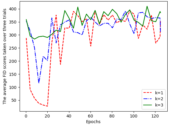
(a) Average FID vs epochs, L$k$StyleGAN-v1.

(b) Average FID vs epochs, L$k$StyleGAN-v2.

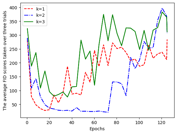
(c) Average FID vs epochs, L$k$StyleGAN-v3.

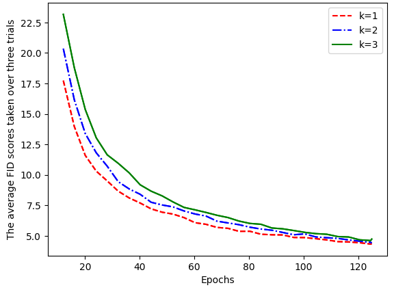
(d) Average FID vs epochs, L$k$StyleGAN-v2-GP.

Figure 1: Evolution of the average FID scores throughout training for L$k$StyleGANs on CelebA (64 $\times$ 64) dataset.

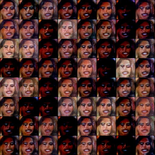
(a) LSStyleGAN-v1: FID score 121.69.

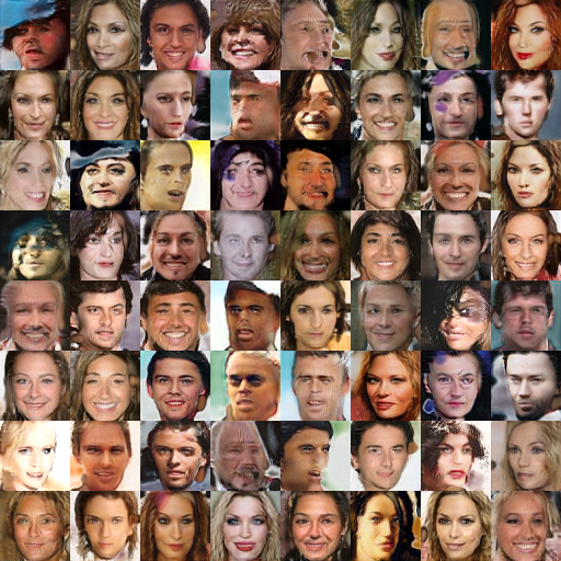
(b) L$k$StyleGAN-v1-1.0: FID score 24.89.

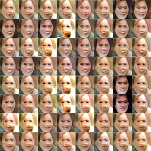
(c) LSStyleGAN-v2: FID score 136.18.

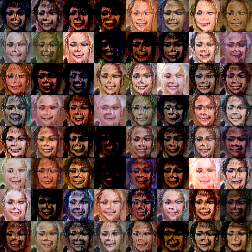
(d) L$k$StyleGAN-v2-1.0: FID score 96.56.

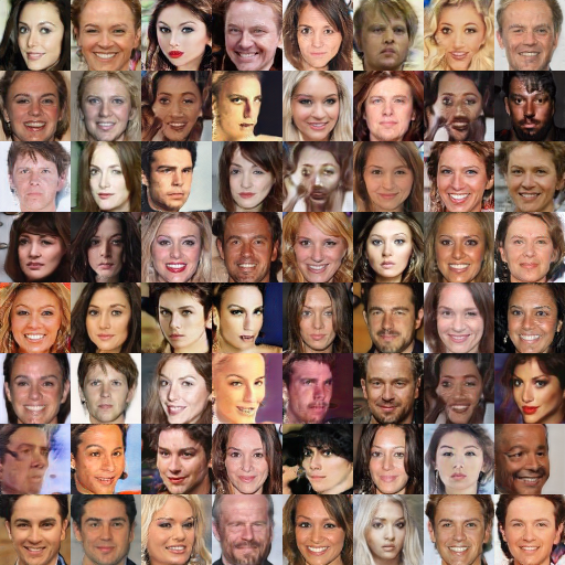
(a) LSStyleGAN-v3: FID score 17.48.

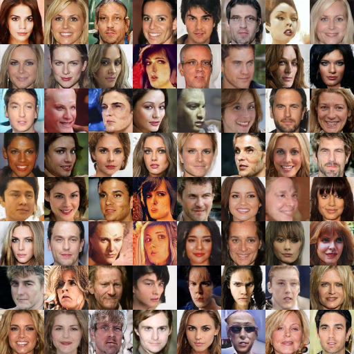
(b) L$k$StyleGAN-v3-1.0: FID score 12.32.

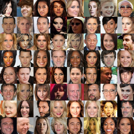
(c) LSStyleGAN-v2-GP: FID score 4.52.

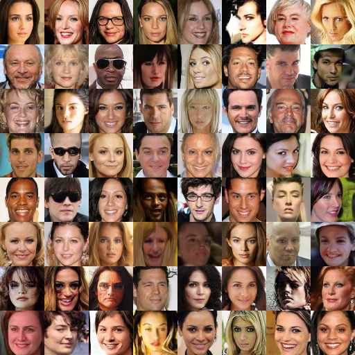
(d) L$k$StyleGAN-v2-1.0-GP: FID score 4.21.

Figure 3: CelebA (64 $\times$ 64) generated images of the best performing L$k$StyleGANs for each version and their LSStyleGAN counterparts for a sample trial.

4 RényiGANs

4.1 Theoretical results

Motivated by generalizing the original GANs, we employ the Rényi cross-entropy loss functional and Jensen-Rényi divergence of order $\alpha>0$, $\alpha\neq 1$, which generalizes the Shannon cross-entropy functional and Jensen-Shannon divergence. Using the same setup and notations as in Section 3, we next present the RényiGANs loss functions.

Definition 6.

The RényiGANs loss functions of order $\bm{\alpha}$, $\alpha>0$, $\alpha\neq 1$, are defined as

$$V_{D}(D,g) = -\mathcal{H}(p_{\mathbf{X}};D)-\mathcal{H}(p_{\mathbf{Z}};1-D\circ g)$$ (20)

$$V_{\alpha,g}(D,g) = -\mathcal{H}_{\alpha}(p_{\mathbf{X}};D)-\mathcal{H}_{\alpha}(p_{\mathbf{Z}};1-D\circ g),$$ (21)

where $\circ$ denotes functional composition, and $\mathcal{H}(\cdot)$ and $\mathcal{H}_{\alpha}(\cdot)$ denote the Shannon and Rényi cross-entropy functionals, respectively (see end of Section 2 before Definition 4).

Note that for RényiGANs, $V_{D}(D,g)=V(D,g)$, where $V(D,g)$ is the original GANs loss function as defined in [21]. The resulting RényiGANs optimization problems consist then of determining:

$$\max_{D}V_{D}(D,g) = \max_{D}\left(-\mathcal{H}(p_{\mathbf{X}};D)-\mathcal{H}(p_{\mathbf{Z}};1-D\circ g)\right)$$ (22)

$$\min_{g}V_{\alpha,g}(D,g) = \min_{g}\left(-\mathcal{H}_{\alpha}(p_{\mathbf{X}};D)-\mathcal{H}_{\alpha}(p_{\mathbf{Z}};1-D\circ g)\right),$$ (23)

The RényiGANs’ generator tries to induce the discriminator to classify the fake images as $1$ by minimizing the negative sum of the two Rényi cross-entropy functionals $\mathcal{H}_{\alpha}(p_{\mathbf{X}};D)$ and $\mathcal{H}_{\alpha}(p_{\mathbf{Z}};1-D\circ g)$, hence generalizing the original GANs loss function by employing a richer $\alpha$-parameterized class of information functionals. Indeed we have that as $\alpha\rightarrow 1$, we recover the original GANs loss function, $V(D,g)$; this is formalized in the following result, whose proof follows directly from Theorem 1.

Theorem 4.

If $V(D,g)<\infty$, then

$$\lim_{\alpha\downarrow 1}V_{\alpha,g}(D,g) = V(D,g).$$ (24)

Moreover, if $\underset{\mathbf{A}\sim p_{\mathbf{X}}}{\mathbb{E}}\left(\frac{1}{D(\mathbf{A})}\right)<\infty$ and $\underset{\mathbf{B}\sim p_{\mathbf{Z}}}{\mathbb{E}}\left(\frac{1}{1-D(g(\mathbf{B}))}\right)<\infty$ then

$$\lim_{\alpha\uparrow 1}V_{\alpha,g}(D,g) = V(D,g).$$ (25)

If the discriminator converges to the optimal discriminator, we next show analytically that for any $\alpha>0$, $\alpha\neq 1$, the optimal generator induces a probability distribution that perfectly mimics the true dataset distribution, as in GANs.

Theorem 5.

Consider problems (22) and (23) for training the discriminator and generator neural networks, respectively. Then

$$D^{*} := \mathrm{argmax}_{D}V_{D}(D,g)=\frac{p_{\mathbf{X}}}{p_{g}+p_{\mathbf{X}}}\ \text{ (a.e.)}.$$ (26)

Furthermore, if $D=D^{*}$, then

$$V_{\alpha,g}(D^{*},g)=2\mathrm{JR}_{\alpha}\left(p_{\mathbf{X}}\|p_{g}\right)-2\log(2)\geq-2\log(2),$$

with equality iff $p_{g}=p_{\mathbf{X}}$ (a.e.).

Proof The proof that the solution to (22) is $D^{*}=p_{\mathbf{X}}/(p_{\mathbf{X}}+p_{g})$ is in [21]. We have that $\underset{\mathbf{B}\sim p_{\mathbf{Z}}}{\mathbb{E}}\left[\left(1-D^{*}(g(\mathbf{B}))\right)^{\alpha-1}\right]=\underset{\mathbf{B}\sim p_{\mathbf{g}}}{\mathbb{E}}\left[\left(1-D^{*}(\mathbf{B}))\right)^{\alpha-1}\right].$ Hence,

$$V_{\alpha,g}(D^{*},g) = \frac{1}{\alpha-1}\left[\log\left(\underset{\mathbf{A}\sim p_{\mathbf{X}}}{\mathbb{E}}\left[\left(D^{*}(\mathbf{A})\right)^{\alpha-1}\right]\right)+\log\left(\underset{\mathbf{B}\sim p_{g}}{\mathbb{E}}\left[\left(1-D^{*}(\mathbf{B})\right)^{\alpha-1}\right]\right)\right]$$

$$= \frac{1}{\alpha-1}\log\left(\underset{\mathbf{A}\sim p_{\mathbf{X}}}{\mathbb{E}}\left[\left(\frac{2p_{\mathbf{X}}(\mathbf{A})}{p_{\mathbf{X}}(\mathbf{A})+p_{g}(\mathbf{A})}\right)^{\alpha-1}\right]\right)$$

$$+\frac{1}{\alpha-1}\log\left(\underset{\mathbf{B}\sim p_{g}}{\mathbb{E}}\left[\left(\frac{2p_{g}(\mathbf{B})}{p_{\mathbf{X}}(\mathbf{B})+p_{g}(\mathbf{B})}\right)^{\alpha-1}\right]\right)-2\log(2)$$

$$= 2\left[\frac{1}{2}\mathrm{D}_{\alpha}\left(p_{\mathbf{X}}\bigg{\|}\frac{p_{\mathbf{X}}+p_{g}}{2}\right)+\frac{1}{2}\mathrm{D}_{\alpha}\left(p_{g}\bigg{\|}\frac{p_{\mathbf{X}}+p_{g}}{2}\right)\right]-2\log(2)$$

$$= 2\mathrm{JR}_{\alpha}\left(p_{\mathbf{X}}\|p_{g}\right)-2\log(2),$$

which is minimized when $p_{g}=p_{\mathbf{X}}$ (a.e.). ∎

This theorem implies that the introduction of the new loss function does not alter the underlying global equilibrium point of RényiGANs when compared to the classical GANs (which use a Shannon-centric loss function), namely that the minimum is theoretically achieved when the generator’s distribution is the true dataset distribution. Using the above Rényi-centric loss function allows control of the shape of the generator’s loss function via the order $\alpha$.

Loss function stability: We close this section by determining the absolute condition number [51] for our Rényi cross-entropy functional $\mathcal{H}_{\alpha}(\cdot;\cdot)$ used in the RényiGAN generator loss function in (21). Such quantity may be a useful to measure loss function stability; in this sense, the loss function is called “stable” if small changes in its argument lead to small changes in its absolute condition number. As our loss function in (21) consists of the (negative) sum of two Rényi cross-entropy functionals, we hence focus on deriving the absolute condition number of our cross-entropy functional $\mathcal{H}_{\alpha}(p;\cdot)$ where $p$ is a fixed probability density with support $\mathcal{R}$. More precisely, the absolute condition number, $\kappa(F)(f(x_{0}))$, of a (Fréchet differentiable) functional $F[f]$ at $f(x_{0})$ (for $x_{0}\in\mathcal{R}$) is defined as [51]

$$\kappa(F)(f(x_{0}))=\left|\frac{\delta F}{\delta f(x_{0})}\right|$$

where $\delta F/\delta f(x)$ is the functional derivative defined via

$$\int\frac{\delta F[f]}{\delta f(x)}\eta(x)\mathrm{d}x:=\frac{\mathrm{d}}{\mathrm{d}\epsilon}F[f+\epsilon\eta]\Big{|}_{\epsilon=0}$$

where $\epsilon\in$ and $\eta$ is an arbitrary function (see [17, Equation (A.15)]). Using similar calculations as in [51], we obtain that the absolute condition number of our Rényi cross-entropy $\mathcal{H}_{\alpha}(p;q(x_{0}))=:F_{\alpha}(q(x_{0}))$ at $q(x_{0})$ is given by

$$\kappa(F_{\alpha})(q(x_{0})))=\frac{p(x_{0})q^{\alpha-2}(x_{0})}{\int_{\mathcal{R}}p(x)q^{\alpha-1}(x)\mathrm{d}\mu},$$ (27)

for $\alpha>0$, $\alpha\neq 1$. For $\alpha<2$, the absolute condition number in (27) approaches infinity as $q(x_{0})\rightarrow 0$. This implies that the generator’s loss function for RényiGAN in (21) produces large gradient updates if $D(x)$ or $1-D(g(z))$ are small. However, for $\alpha\geq 2$, the absolute condition number is bounded and hence the generator’s gradient updates are stable for any $D(x)$ and $1-D(g(z))$. In contrast, it is shown in [51] that the Shannon cross-entropy (which is used in the original GAN loss function, see (20)) is unstable if $D(x)$ or $1-D(g(z))$ are small. Finally as noted in [51], we emphasize that while we have ascertained a notion of stability for our Rényi-type loss function for $\alpha\geq 2$ (which was observed in our experiments), there are other factors that play an important role in a GAN’s overall stability (including the system architecture and the employed gradient decent technique).

4.2 Experiments

4.2.1 Methods

The $28\times 28\times 1$ MNIST [31], $64\times 64\times 3$ CelebA, and $128\times 128\times 3$ CelebA [36] datasets were used to test the RényiGANs loss functions. As in Section 3, FID scores were used to evaluate the quality of the generated images and to compare the rate at which the new networks converge to their optimal scores. The structure of the generator and discriminator neural networks were kept constant when testing on each dataset; see Section A and Algorithm 2 in the Appendix for details. For comparison, the classical (Shannon-centric) GANs loss functions were also tested.

We denote RényiGAN-$\alpha$ as RényiGANs that use a fixed value value of $\alpha$ during training (see Algorithm 2 in the Appendix). For the MNIST dataset, in addition to implementing RényiGAN-$\alpha$, RényiGANs were tested while altering $\alpha$ for every epoch of the simulation. This changes the shape of the loss function of the generator. However, changing $\alpha$ does not affect the global minimum as for all $\alpha>0$, the global minimum is realized when $p_{\mathbf{X}}=p_{g}$. Assuming that a generator $p_{g}\neq p_{\mathbf{X}}$ is realized such that it is not a local minimum of $V_{\alpha}(D,g)$ for all $\alpha>0$, then changing $\alpha$ every epoch creates non-zero gradients at previous local minimums, hence helping the algorithm overcome the problem of getting stuck in local minimums. We denote this as RényiGAN-$[\beta_{1},\beta_{2}]$, with the $\alpha$ value starting at $\alpha=\beta_{1}$ and ranging over the interval $[\beta_{1},\beta_{2}]$.

One goal was to examine whether the generalized (Rényi-based) loss functions have appreciable benefits over the classical GANs loss function and whether it provides better training stability. It is known that deep convolutional GANs (DCGANs) exhibit stability issues which motivate us to investigate modifications to the loss functions involving the addition of the $L_{1}$ norm. Specifically, those stability issues arise when the GANs generator tries to minimize its cost function to $-\infty$ by labelling $D(g(z))=1$ for all fake images $g(z)$. In the early stages of the simulations, if the discriminator does not successfully converge to its optimal value and the generator is able to induce the discriminator to label poorly generated images as $1$, then in later epochs, once the discriminator converges to its optimal value and is able to tell apart real and fake images perfectly, the generator’s loss function produces no gradients. In other words, the optimal discriminator does not allow the generator to improve the quality of fake images which leads to the discriminator winning problem. A similar argument was noted in [6]. Thus to remedy the stability problem, a modified RényiGANs’ generator’s loss function was tested by taking the $L_{1}$ norm of its deviation from $-2\log(2)$, its theoretically minimal value predicted by Theorem 5; this yields the following minimization problem for the generator network:

$$\min_{g}\Big{|}V_{\alpha,g}(D,g)-(-2\log 2)\Big{|}$$ (28)

Using the $L_{1}$ norm ensures that the generator’s loss function does not try to label its images as $1$, but rather tries to label them as $1/2$. Hence in the early training stages, if the generator converges to images that are labelled $1/2$ by the discriminator, then in the later stages, if the discriminator converges to its theoretical optimal value (given in Theorem 5), the generator’s loss function has non-zero gradient updates and is only able to label fake images as $1/2$ when $p_{g}=p_{\mathbf{X}}$. Note that the altered loss function in (28) translates into composing the L$k$GAN error function using $k=1$ and $\gamma=-\log(2)$ (see Section 3) with the RényiGAN loss function. Indeed, the improved stability property of L$k$GANs (particularly when $k=1$) is the main motivation for using this $L_{1}$ normalization. We denote the resulting scheme under (28) by RényiGAN-$L_{1}$. The RényiGANs and classical GANs loss functions were also tested with and without the addition of simplified gradient penalties. We denote this as RényiGAN-GP and DCGAN-GP.

In summary, we considered the evaluation of four versions of the algorithm with six different loss functions within each version. Version $1$ has RényiGAN-$0.5$, RényiGAN-$3.0$, RényiGAN-$[0,0.9]$, RényiGAN-$[0,3.0]$, RényiGAN-$[1.1,4]$, and DCGAN. Version $2$ has the six original loss functions with $L_{1}$ normalization, Version $3$ has gradient penalty, and Version $4$ has gradient penalty and $L_{1}$ normalization incorporated in the loss functions.

For the MNIST dataset, seeds $123$, $5005$, $1600$, $199621$, $60677$, $20435$, $15859$, $33764$, $79878$, $36123$ were used for trials $1$ to $10$, respectively. For the SGD algorithm, the Adam optimizer with a learning rate of $\alpha_{Adam}=2\times 10^{-4}$, $\beta_{1}=0.5$, $\beta_{2}=0.999$, and $\epsilon=1\times 10^{-7}$ was used for the networks as recommended by [49]. The batch size was chosen to be $100$ for the $60,000$ MNIST images. The networks were trained on the MNIST dataset for a total number of $250$ epochs, or 15 million images.

For CelebA, as in Section 3, we ran three trials with seeds 1000, 2000, and 3000 for trials 1, 2, and 3 respectively. For comparison, the original StyleGAN with the classical GANs loss function was implemented. The publicly available StyleGAN code from [27] was modified to test the RényiGANs loss functions. We refer to this as RényiStyleGANs. RényiStyleGANs were implemented for $\alpha\in\{3.0,9.0\}$. RényiStyleGANs and StyleGANs with the simplified gradient penalty, referred to as RényiStyleGAN-GP and StyleGAN-GP, respectively, were also tested. The original StyleGAN architectural defaults were left in place with a batch size of 128. As in Section 3.2.1, the resolution of the generated images for RényiStyleGANs and StyleGAN was fixed at $64\times 64\times 3$ or at $128\times 128\times 3$ throughout training. The same Adam optimizer parameters were used as specified in Section 3.2.1 and the systems were trained for 25 million images (roughly 120 epochs). One NVIDIA GP$100$ GPU and two Intel Xeon $2.6$ GHz E$7-8867$ v$3$ CPUs were used for RényiGANs and DCGANs, and four NVIDIA V 100 GPUs were used for RényiStyleGANs and StyleGANs.

4.2.2 MNIST results

A total of ten trials were run while controlling the random seed in each trial. We did not use the Inception network to calculate the FID scores as it is not trained on classifying handwritten MNIST images. Instead, the scores were computed using the raw real and fake images under multivariate Gaussian distributions. The average and variance over ten trials of the best FID scores (i.e., lowest score over all epochs), and the average and variance of the epoch when the best FID score is achieved are presented for a representative subset of the tested systems in Table 2. A few variants of RényiGANs converged to meaningful results, which we show in Table 3. Finally, samples of MNIST generated images are given in Figure 4.

Table 2: RényiGANs MNIST experiments: the average and variance of the best FID scores and the average and variance of the epoch this occurs (over 10 trials).

	Average best FID score	Best FID scores variance	Average epoch	Epoch variance
RényiGAN-$3.0$	52.99	292.71	32.70	92.21
RényiGAN-$\mathbf{[0,3]}$	41.59	693.61	95.40	9096.64
DCGAN	59.061	$\mathbf{2.01\times 10^{-28}}$	13.00	0.80
RényiGAN-$3.0$-$L_{1}$	1.80	2.95 $\times 10^{-3}$	86.80	4611.16
RényiGAN-$\mathbf{[0,3]}$-$\mathbf{L_{1}}$	1.77	4.90 $\times 10^{-3}$	36.10	36.80
DCGAN-$L_{1}$	1.93	3.83 $\times 10^{-3}$	52.30	2605.61
RényiGAN-GP-$3.0$	1.36	2.51 $\times 10^{-3}$	209.10	751.09
RényiGAN-GP-$[0,3]$	1.41	3.09 $\times 10^{-3}$	201.90	1209.69
DCGAN-GP	1.36	$\mathbf{1.45\times 10^{-3}}$	225.20	342.56
RényiGAN-GP-$\mathbf{3.0}$-$\mathbf{L_{1}}$	1.17	$3.62\times 10^{-3}$	221.70	609.61
RényiGAN-GP-$[0,3]$-$L_{1}$	1.22	6.33 $\times 10^{-3}$	224.10	1075.09
DCGAN-GP-$L_{1}$	1.18	1.58 $\times 10^{-3}$	200.50	1263.05

Table 3: The average and variance best FID scores for RényiGANs that generated meaningful MNIST images and the average and variance of the epoch when this occurs.

	Average best FID score	Best FID scores variance	Average epoch	Epoch variance
RényiGAN-3.0	1.66	0.00	60.00	0.00
RényiGAN-[0,3]	1.36	3.81 ${\times 10^{-3}}$	240.00	6.00

4.2.3 CelebA results

We demonstrate our results on both $64\times 64\times 3$ and $128\times 128\times 3$ CelebA images. For the $64\times 64\times 3$ case, three trials were run for a few $\alpha$ values for RényiStyleGANs. RényiStyleGANs with and without the simplified gradient penalty were also tested. Only RényiStyleGAN-3.0-GP was tested because the addition of the simplified gradient penalties increased computing time. The FID scores were calculated every $80,000$ images. The average and variance of best FID scores taken over the three trials are presented in Table 4. We present the plots of the average FID scores taken over the three trials versus epochs in Figure 5(a) and 5(b). Sample generated images of one of the trials for RényiStyleGAN and StyleGAN are shown in Figure 6.

For the $128\times 128\times 3$ case, three trials were also run for RényiStyleGAN and StyleGAN with the FID scores calculated every $60,000$ images. The average and variance of best FID scores taken over the three trials are shown in Table 5. The average FID scores taken over the three trials are plotted versus epochs in Figure 5(c). Sample generated images of one of the trials for RényiStyleGAN and StyleGAN are given in Figure 7.

Table 4: RényiStyleGANs CelebA (64 $\times$ 64) experiments: the average and variance of the best FID score and the average and variance this occurs (over 3 trials).

	Average best FID score	Best FID score variance	Average epoch	Epoch variance
RényiStyleGAN-3.0	9.80	$\mathbf{5.93\times 10^{-2}}$	112.54	75.38
RényiStyleGAN-9.0	10.38	2.12	115.22	111.28
StyleGAN	14.60	12.48	93.78	477.53
RényiStyleGAN-3.0-GP	3.88	$\mathbf{1.84\times 10^{-3}}$	122.05	4.35
StyleGAN-GP	3.92	9.06 $\times 10^{-3}$	119.37	58.94

Table 5: RényiStyleGANs CelebA (128 $\times$ 128) experiments: the average and variance of the best FID score and the average and variance this occurs (over 3 trials).

	Average best FID score	Best FID score variance	Average epoch	Epoch variance
RényiStyleGAN-3.0	30.47	480.69	72.50	565.68
RényiStyleGAN-9.0	17.34	3.40	93.64	371.08
StyleGAN	39.11	962.46	48.33	918.63

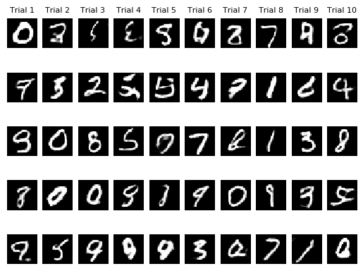
(a) DCGAN-$L_{1}$ sample images.

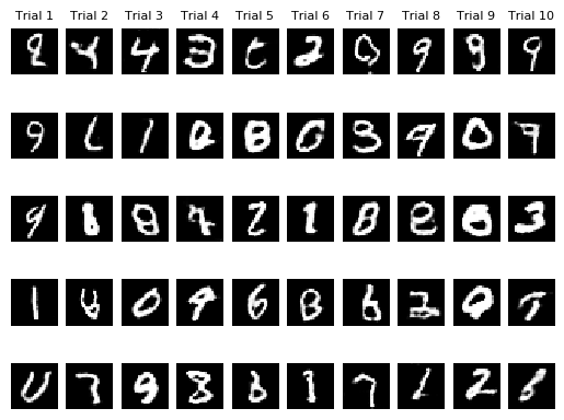
(b) RényiGAN-$[0,3]$-$L_{1}$ sample images.

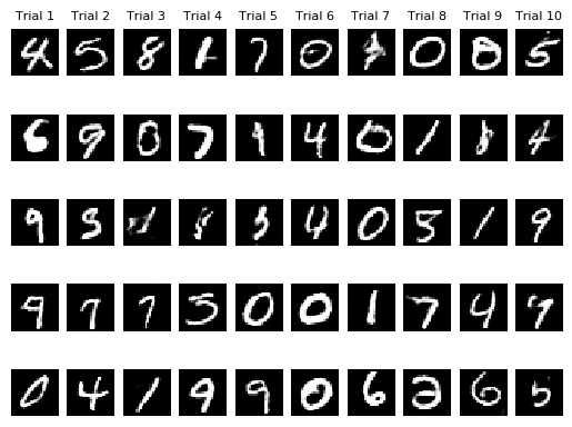
(c) DCGAN-GP sample images.

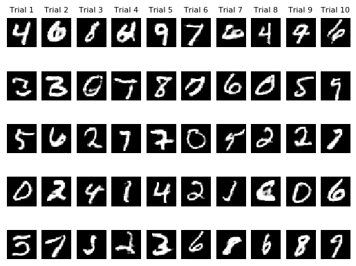
(d) RényiGAN-GP-$3.0$ sample images.

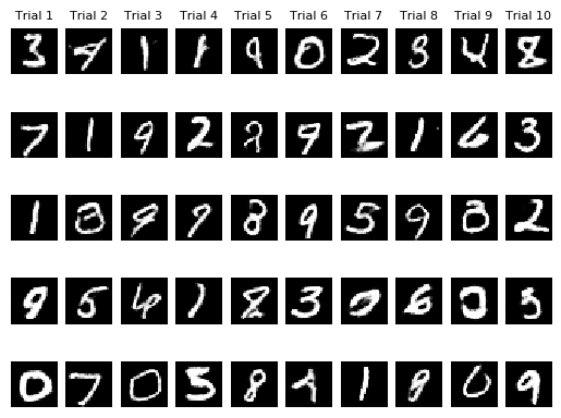
(e) DCGAN-GP-$L_{1}$ sample images.

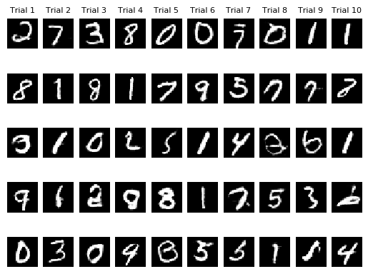
(f) RényiGAN-GP-$3.0$-$L_{1}$ sample images.

Figure 4: MNIST generated images of the best performing RényiGANs and DCGANS in terms of FID scores.

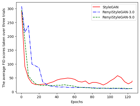
(a) Average FID vs epochs, RényiStyleGANs and StyleGANs for CelebA ($64\times 64$).

(b) Average FID vs epochs, RényiStyleGAN-GPs and StyleGAN-GPs for CelebA ($64\times 64$).

(c) Average FID vs epochs, RényiStyleGANs and StyleGANs for CelebA ($128\times 128$).

Figure 5: Evolution of the average FID scores throughout training for RényiStyleGANs.

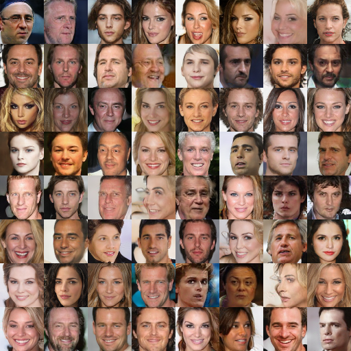
(a) StyleGAN: FID score 16.20.

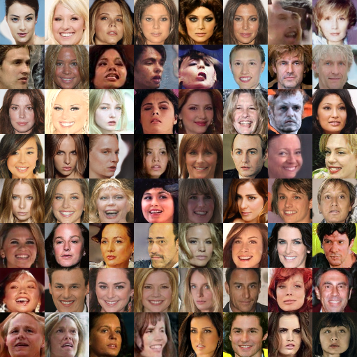
(b) RényiStyleGAN-3.0: FID score 9.67.

(c) StyleGAN-GP: FID score 4.06.

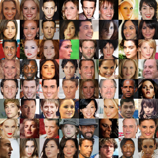
(d) RényiStyleGAN-3.0-GP: FID score 3.91.

Figure 6: CelebA (64 $\times$ 64) generated images of the best performing RényiStyleGANs for each version and their StyleGAN counterparts for a sample trial.

(a) StyleGAN: FID score 19.72.

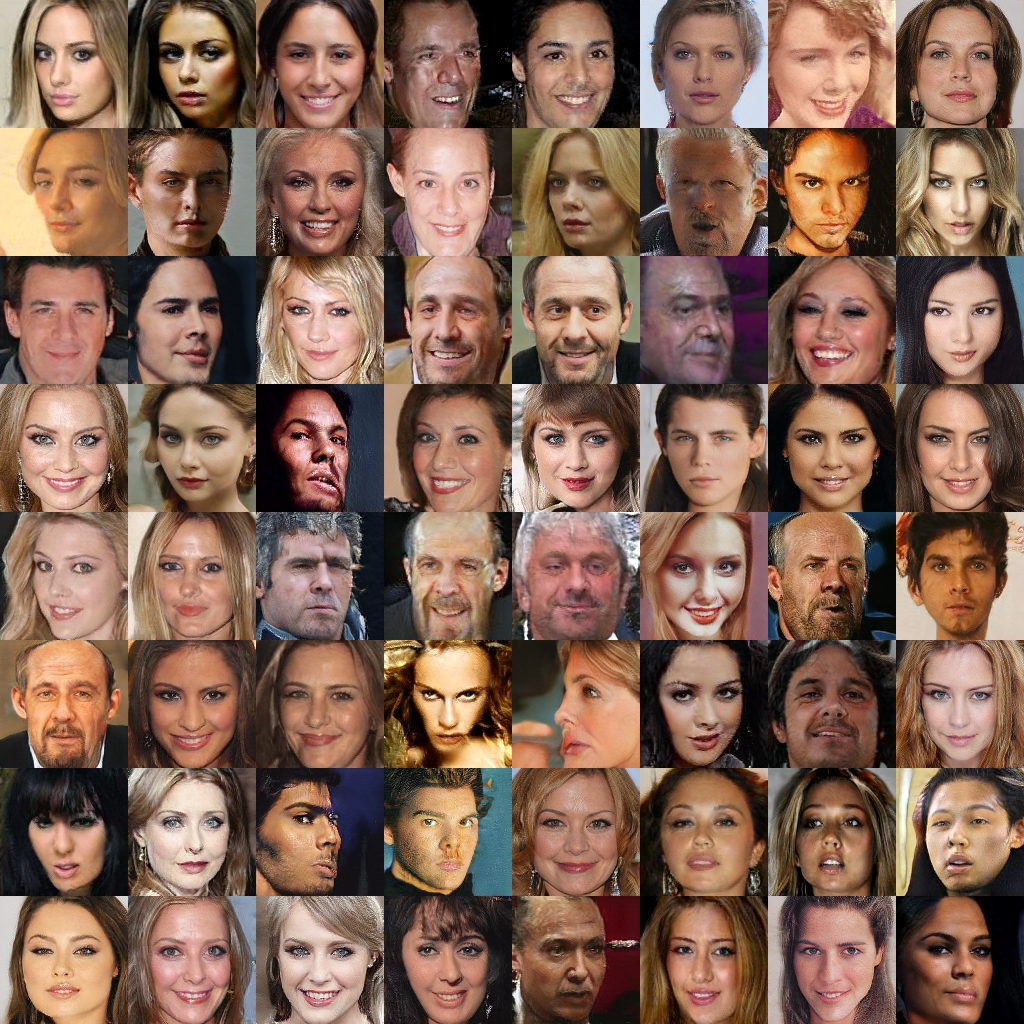
(b) RényiStyleGAN-3.0: FID score 15.05.

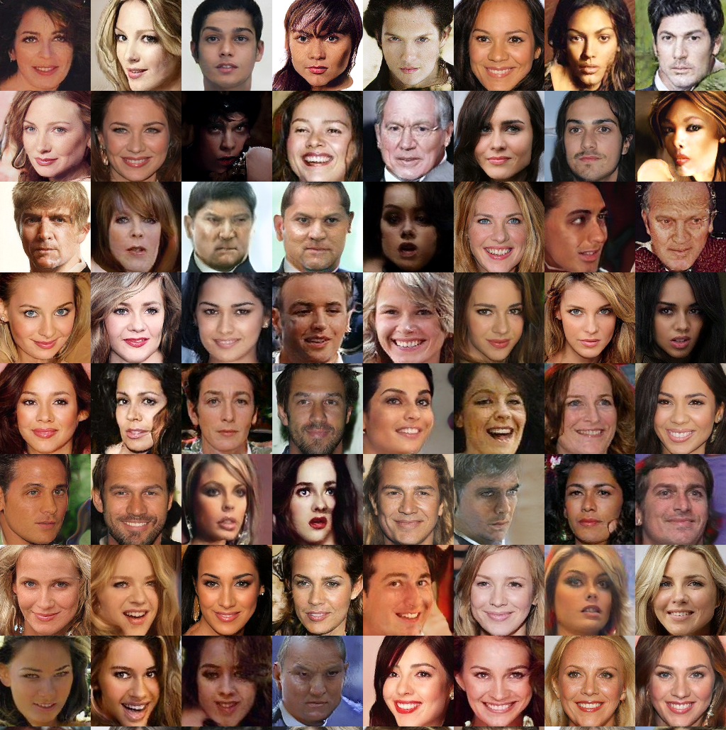
(c) RényiStyleGAN-9.0: FID score 15.41.

Figure 7: CelebA (128 $\times$ 128) generated images of the best performing RényiStyle-GANs for each version and their StyleGAN counterparts for a sample trial.

4.3 Discussion

4.3.1 MNIST

The DCGAN baseline exhibited unstable training as was expected and the addition of the Rényi loss was able to ameliorate convergence but had similar instabilities. More specifically, RényiGAN-$[0,3]$ converged in three out of ten trials, achieving an average best FID scores of $1.36$, while DCGAN experienced mode collapse in all ten trials. This FID score is comparable to that of applying simplified gradient penalty to the network. Note that these networks took an average time of 42.33 minutes to train for one trial.

Applying the $L_{1}$ normalization drastically improved the convergence of all networks with no computational overhead. In fact, on average over $250$ epochs and $10$ trials, adding $L_{1}$ normalization on average decreased the training time for one trial to 41.79 minutes, which is a decrease of $1.27\%$. This is expected as the $L_{1}$ normalization is similar to the L$k$GANs generator loss function when $k=1$ and $\gamma=-\log(2)$, which, as we have shown in Section 3, improves training stability. Using $L_{1}$ normalization also has the added benefit of networks converging to an optimal FID value in fewer epochs than any other convergent networks across all versions. We note that RényiGAN-$[0,3]$-$L_{1}$ outperformed all other loss functions in Version 2 and it was sufficient to train it within $50$ epochs. The development of a rigorous theory that describes this phenomenon is an interesting future direction to better understand the dynamics of GANs.

In Version $3$, RényiGAN-GP-$[1.1,4]$ performed among the best compared to other RényiGAN-GP variants, with an identical performance to DCGAN-GP. Moreover, on average it converged to its best FID score in fewer epochs than DCGAN-GP. Note, however, that the use of gradient penalty increased the average computation time to 47.54 minutes for a single trial, an increase of $12.30\%$ compared to Version 1. The best performing network in terms of FID score was RényiGAN-GP-$3.0$-$L_{1}$, seen in the Version 4 results of Table 2. Note that RényiGAN-GP-$0.5$-$L_{1}$, RényiGAN-GP-$3.0$-$L_{1}$, RényiGAN-GP-$[0,0.9]$-$L_{1}$, and DCGAN-GP-$L_{1}$ exhibited quite similar FID scores. However, on average, DCGAN-GP-$L_{1}$ converged to its optimal FID score in fewer epochs than its counterparts. On average, these networks with gradient penalty and $L_{1}$ normalization took 47.17 minutes to train for a single trial, which is a slight decrease in computational time compared to applying simplified gradient penalties only.

In summary, the extra degree of freedom provided by the order $\alpha$ resulted in equivalent or better FID scores in fewer epochs when using either $L_{1}$ normalization or the simplified gradient penalty. The greatest advantage of RényiGANs when applied to MNIST was its ability to converge to realistic and diverse generated images quicker than DCGANs in most versions.

4.3.2 CelebA

For $64\times 64\times 3$ CelebA, we observed that RényiStyleGANs (with $\alpha>1$) outperform StyleGANs in terms of FID scores, with setting $\alpha=3.0$ achieving the best average FID score. However, further investigation on the best range of values of $\alpha$ for RényiStyleGANs is necessary.

Comparing the performance of RényiStyleGAN to StyleGAN in Figure 5(a) reveals that RényiStyleGAN performs consistently and does not display the erratic unstable behaviour of regular StyleGANs. One explanation for the difference in performance dynamics is that the Rényi loss dampens the loss of each individual sample in the batch, reducing the effect of samples that may be given spurious gradient directions. Combined with our use of the Adam optimizer to keep track of the gradient variance, the overall effect that dampening has on the entire objective function is normalized out, while still maintaining the benefit of dampening individual samples from the generator. Additionally, as we close the gap between StyleGANs with and without gradient penalty, one benefit of not needing gradient penalty was the significant reduction in computation time: RényiStyleGAN-$3.0$ took 25.63 hours without gradient penalty and 31.8 hours with gradient penalty, yielding a 24$\%$ increase in computation time when using gradient penalty. Lastly, both RényiStyleGAN-GP and StyleGAN-GP performed identically; see Figure 5(b).

For the $128\times 128\times 3$ CelebA dataset, we observed that StyleGAN converged to meaningful results in two out the three trials, whereas both RényiStyleGAN-3.0 and RényiStyleGAN-9.0 converged to meaningful results in all three trials. Furthermore, Figure 5(c) confirms that for a large $\alpha$ value, RényiStyleGANs does not behave erratically during training. Although StyleGAN generated high quality images early in training, it suffered from mode collapse as training continued. In contrast, both RényiStyleGANs typically generated high quality images as training continued, though the FID of one RényiStyleGAN-3.0 run increased as training continued and consequently dragged the average FID up in Figure 5(c). This behaviour is useful as it bridges the gap between StyleGANs with and without gradient penalty.

4.4 Comparing RényiGANs and L$k$GANs

We observe that the quality of generated images in terms of FID scores was better for RényiGANs than for L$k$GANs, irrespective of the tested datasets. For the $64\times 64\times 3$ CelebA dataset, the best performing L$k$StyleGAN had parameters $k=1.0$ with $a=0$, $b=1$, and $c=1$, which realized an FID score of $18.83$. Although it outperformed its LSStyleGAN counterpart, L$k$StyleGAN achieved a higher average FID score than RényiStyleGAN. Indeed, RényiStyleGAN with $\alpha=3.0$ and $\alpha=9.0$ had FID scores of $9.80$ and $10.38$, respectively. The use of gradient penalty showed a similar pattern; RényiStyleGAN-$3.0$ had a lower average FID score compared to the best performing L$k$StyleGAN (3.88 vs. 4.31). Similarly, for the MNIST dataset, the best performing L$k$GAN achieved an average FID score of $3.13$ (not shown here, see Footnote 5), whereas the best performing RényiGAN achieved an average FID score of $1.77$. Hence experiments show that RényiGANs consistently outperformed L$k$GANs in terms of generated image quality.

Furthermore, RényiGANs outperformed L$k$GANs in terms of training stability. For the CelebA dataset, RényiStyleGANs did not exhibit the erratic fluctuations in image quality of L$k$StyleGANs during training. This is evident when comparing the plots of average FID score versus epochs for L$k$StyleGANs and RényiStyleGANs in Figures 1 and 5, respectively. Indeed RényiGANs’ increased training stability bridges the gap between GANs with and without gradient penalty. Finally, under gradient penalty, both L$k$StyleGANs and RényiStyleGANs performed similarly.

5 Conclusion

We introduced two new GAN generator loss functions. We first analyzed and implemented L$k$GANs, which generalize LSGANs (for $k\neq 2$). We showed that the theoretical minimum when solving the generator optimization problem for L$k$GANs is achieved when the generator’s distribution matches the true data distribution. Using experiments on the CelebA dataset under the StyleGAN architecture, the new L$k$GANs loss functions conferred greater training stability and better generated image quality than LSGANs. Experiments also revealed new research directions, such as analyzing the effects of the L$k$GAN parameters and the order $k$ on performance.

We next proposed, analyzed, and implemented a GAN generator loss function based on Rényi cross-entropy measures of order $\alpha$ ($\alpha>0$ and $\alpha\neq 1$). We showed that the classical GANs analytical minimax result expressed in terms of minimizing the Jensen-Shannon divergence between the generator and the unconstrained discriminator distributions can be generalized for any $\alpha$ in terms of the broader Jensen-Rényi divergence, with the original GANs loss function provably recovered in the limit of $\alpha$ approaching 1. We demonstrated via experiments on MNIST and CelebA datasets that the Rényi-based loss function (which was analytically shown to be stable for $\alpha\geq 2$) yields performance improvements over the original GANs loss function in terms of the quality of the generated images and training stability. In particular, we observed that RényiGANs used with $L_{1}$ normalization on MNIST images does not need gradient penalty to reduce the GAN mode collapse problem. Furthermore, RényiStyleGANs (used on CelebA images) provide more robust convergence dynamics than StyleGANs and can dispose of using gradient penalty without affecting image fidelity while requiring considerably less training time. Overall, the performance of RényiGAN/RényiStyleGAN was superior to those of L$k$GAN/L$k$StyleGAN by virtue of the Rényi cross-entropy loss function. For future research, it would be useful to examine the effects of the Rényi order $\alpha$ on the optimal choice of network architectures and parameters. Finally, we note that the L$k$- and Rényi-centric methods studied in this work can be judiciously adopted to other deep learning neural network architectures.

Appendix A Neural network architectures

The StyleGAN architecture were taken directly from [27]. The architectures for the MNIST dataset are detailed below in Tables 6 and 7. We used the architecture guidelines provided by [49] and the GANs tutorial in [1]. We shorten some of the common terms used to describe the layers of the networks. A fully connected layer in a neural network is denoted by FC, while we have used upconv. to denote a convolution layer that is specifically padded to increase the dimensions of its input image. The bias in each upconv. layer was not used in an effort to reduce the amount of parameters and the computational training time. The parameters of the neural networks were initialized by sampling a Gaussian random variable with mean $0$ and standard deviation $0.01$.

Table 6: The generator’s architecture for MNIST dataset.

Generator
Input multivariate Gaussian noise vector of size $784$ with mean $\mathbf{0}$
and a covariance matrix that is the identity matrix of size $784\times 784$.
FC to $12,544$ neurons.
Reshape into $7\times 7\times 256$ image.
$5\times 5$ upconv. $128$ LeakyRELU, batchnorm.
$5\times 5$ upconv. $64$ LeakyRELU, stride 2, batchnorm.
$5\times 5$ upconv. $1$ channel, $\tanh$ activation.

Table 7: The discriminator’s architecture for MNIST dataset.

Discriminator
Input $28\times 28\times 1$ grey image.
$5\times 5$ conv. $64$ LeakyRELU, stride 2, batchnorm,
dropout $0.3$.
$5\times 5$ conv. $128$ LeakyRELU, stride 2, batchnorm,
dropout $0.3$.
FC to one output, $\frac{1}{1+e^{-x}}$ activation.

Appendix B Algorithms

We present the algorithms for L$k$GANs below. For the CelebA dataset, the constants of the algorithms are $n=125$ epochs or 25 million images and the batch size $m=126$.

We also present the algorithms for RényiGANs. For the MNIST dataset, the constants of the algorithms are $n=100$ epochs or 6 million images and batch size $m=100$. For the CelebA dataset, the constants of the algorithms are $n=125$ epochs or 25 million images and the batch size $m=126$.

Algorithm 1 Overview of L$k$GAN-v$1$-$k$ and L$k$GAN-v$2$-$k$ algorithms with and without the simplified gradient penalty.

Initialize neural networks.

Fix number of epochs $n$.

for $i=0$ to $n-1$ do

   Sample batch size of $m$ noise samples $\{\bm{z}_{1},\ldots,\bm{z}_{m}\}$ from noise prior $p_{\mathbf{Z}}$

   Sample batch size of $m$ examples $\{\mathbf{x}_{1},\ldots,\mathbf{x}_{m}\}$ from the true distribution $p_{\mathbf{X}}$

   Update the discriminator by descending its gradient without the simplified gradient penalty:

$$\nabla_{\bm{\tilde{\theta}}}\left(\frac{1}{m}\sum_{i=1}^{m}\left[\frac{1}{2}(D(\mathbf{x}_{i})-b)^{2}+\frac{1}{2}(D(g(\bm{z}_{i}))-a)^{2}\right]\right),$$

or with the simplified gradient penalty:

$$\nabla_{\bm{\tilde{\theta}}}\Bigg{(}\frac{1}{m}\sum_{i=1}^{m}\left[\frac{1}{2}(D(\mathbf{x}_{i})-b)^{2}+\frac{1}{2}(D(g(\bm{z}_{i}))-a)^{2}\right]$$

$$+5\left(\frac{1}{m}\sum_{i=1}^{m}\left\|\nabla_{\mathbf{x}}\log\left(\frac{D(\mathbf{x})}{1-D(\mathbf{x})}\right)\bigg{|}_{\mathbf{x}=\mathbf{x}_{i}}\right\|_{2}^{2}\right)\Bigg{)}.$$

   Update the generator by descending its gradient:

$$\nabla_{\bm{\theta}}\left(\frac{1}{m}\sum_{i=1}^{m}|D(g(\bm{z}_{i}))-c|^{k}\right),$$

end for

Algorithm 2 Overview of RényiGAN-$\alpha$, RényiGAN-$\alpha$-$L_{1}$, and RényiGAN-GP-$\alpha$-$L_{1}$ algorithms

Initialize neural networks.

Fix number of epochs $n$.

for $i=0$ to $n-1$ do

   Sample batch size of $m$ noise samples $\{\bm{z}_{1},\ldots,\bm{z}_{m}\}$ from noise prior $p_{\mathbf{Z}}$

   Sample batch size of $m$ examples $\{\mathbf{x}_{1},\ldots,\mathbf{x}_{m}\}$ from the true distribution $p_{\mathbf{X}}$

   Update the discriminator by descending its stochastic gradient without the simplified gradient penalty:

$$\nabla_{\bm{\tilde{\theta}}}\bigg{(}-\frac{1}{m}\sum_{i=1}^{m}\big{[}\log D(\mathbf{x}_{i})+\log(1-D(g(\bm{z}_{i})))\big{]}\bigg{)},$$

or with the simplified gradient penalty:

$$\nabla_{\bm{\tilde{\theta}}}\Bigg{(}-\frac{1}{m}\sum_{i=1}^{m}\big{[}\log D(\mathbf{x}_{i})+\log(1-D(g(\bm{z}_{i})))\big{]}$$

$$+5\left(\frac{1}{m}\sum_{i=1}^{m}\left\|\nabla_{\mathbf{x}}\log\left(\frac{D(\mathbf{x})}{1-D(\mathbf{x})}\right)\bigg{|}_{\mathbf{x}=\mathbf{x}_{i}}\right\|_{2}^{2}\right)\Bigg{)},$$

and update the generator by descending its stochastic gradient without $L_{1}$ normalization:

$$\nabla_{\bm{\theta}}\frac{1}{\alpha-1}\log\Bigg{[}\left(\frac{1}{m}\sum_{i=1}^{m}[1-D(g(\bm{z}_{i}))]^{\alpha-1}\right)\Bigg{]},$$

or with $L_{1}$ normalization:

$$\nabla_{\bm{\theta}}\Bigg{|}\frac{1}{\alpha-1}\log\Bigg{[}\left(\frac{1}{m}\sum_{i=1}^{m}[1-D(g(\bm{z}_{i}))]^{\alpha-1}\right)\Bigg{]}+\log(2)\Bigg{|},$$

end for

References

- [1] Martín Abadi, Ashish Agarwal, Paul Barham, Eugene Brevdo, Zhifeng Chen, Craig Citro, Greg S. Corrado, Andy Davis, Jeffrey Dean, Matthieu Devin, Sanjay Ghemawat, Ian Goodfellow, Andrew Harp, Geoffrey Irving, Michael Isard, Yangqing Jia, Rafal Jozefowicz, Lukasz Kaiser, Manjunath Kudlur, Josh Levenberg, Dandelion Mané, Rajat Monga, Sherry Moore, Derek Murray, Chris Olah, Mike Schuster, Jonathon Shlens, Benoit Steiner, Ilya Sutskever, Kunal Talwar, Paul Tucker, Vincent Vanhoucke, Vijay Vasudevan, Fernanda Viégas, Oriol Vinyals, Pete Warden, Martin Wattenberg, Martin Wicke, Yuan Yu, and Xiaoqiang Zheng. TensorFlow: Large-scale machine learning on heterogeneous systems, 2015. Software available from tensorflow.org.
- [2] Alessandro Achille and Stefano Soatto. Where is the information in a deep neural network? ArXiv:1905.12213, 2019.
- [3] Fady Alajaji, Po-Ning Chen, and Ziad Rached. Csiszár’s cutoff rates for the general hypothesis testing problem. IEEE Transactions on Information Theory, 50(4):663–678, 2004.
- [4] Alexander A. Alemi, Ian Fischer, Joshua V Dillon, and Kevin Murphy. Deep variational information bottleneck. In Proceedings of the 5th International Conference on Learning Representations, pages 1–19, 2017.
- [5] Erdal Arikan. An inequality on guessing and its applications to sequential decoding. IEEE Transactions on Information Theory, 42(1):99–105, 1996.
- [6] Martin Arjovsky, Soumith Chintala, and Léon Bottou. Wasserstein generative adversarial networks. In Proceedings of the 34th International Conference on Machine Learning, volume 70, pages 214–223, 2017.
- [7] Moshe Ben-Bassat and Joseph Raviv. Rényi’s entropy and the probability of error. IEEE Transactions on Information Theory, 24(3):324–331, 2006.
- [8] Himesh Bhatia, William Paul, Fady Alajaji, Bahman Gharesifard, and Philippe Burlina. Rényi Generative Adversarial Networks. ArXiv:2006.02479, 2020.
- [9] Philippe Burlina, Neil Joshi, William Paul, Katia D Pacheco, and Neil M Bressler. Addressing artificial intelligence bias in retinal disease diagnostics. arXiv preprint arXiv:2004.13515, 2020.
- [10] Lorne L. Campbell. A coding theorem and Rényi’s entropy. Information and Control, 9:423–429, 1965.
- [11] Liqun Chen, Shuyang Dai, Yunchen Pu, Erjin Zhou, Chunyuan Li, Qinliang Su, Changyou Chen, and Lawrence Carin. Symmetric variational autoencoder and connections to adversarial learning. In Proceedings of the 22nd International Conference on Artificial Intelligence and Statistics, volume 84 of Proceedings of Machine Learning Research, pages 661–669, 2018.
- [12] Xi Chen, Yan Duan, Rein Houthooft, John Schulman, Ilya Sutskever, and Pieter Abbeel. InfoGAN: Interpretable representation learning by information maximizing generative adversarial nets. In Advances in Neural Information Processing Systems, pages 2172–2180, 2016.
- [13] Thomas A. Courtade and Sergio Verdú. Cumulant generating function of codeword lengths in optimal lossless compression. In Proceedings of the IEEE International Symposium on Information Theory, pages 2494–2498, 2014.
- [14] Antonia Creswell, Tom White, Vincent Dumoulin, Kai Arulkumaran, Biswa Sengupta, and Anil A Bharath. Generative adversarial networks: An overview. IEEE Signal Processing Magazine, 35(1):53–65, 2018.
- [15] Imre Csiszár. Information-type measures of difference of probability distributions and indirect observations. Studia Sci. Math. Hungarica, 2:299–318, 1967.
- [16] Imre Csiszár. Generalized cutoff rates and Rényi’s information measures. IEEE Transactions on Information Theory, 41(1):26–34, 1995.
- [17] Eberhard Engel and Reiner M. Dreizler. Density Functional Theory. Springer, 2011.
- [18] Amedeo R. Esposito, Michael Gastpar, and Ibrahim Issa. Robust generalization via -mutual information. In Proceedings of the International Zurich Seminar on Information and Communication, pages 96–100, 2020.
- [19] Farzan Farnia and David Tse. A convex duality framework for GANs. In Advances in Neural Information Processing Systems 31, pages 5248–5258, 2018.
- [20] Ian Goodfellow. NIPS 2016 Tutorial: Generative Adversarial Networks. ArXiv:1701.00160, 2016.
- [21] Ian Goodfellow, Jean Pouget-Abadie, Mehdi Mirza, Bing Xu, David Warde-Farley, Sherjil Ozair, Aaron Courville, and Yoshua Bengio. Generative adversarial nets. In Advances in Neural Information Processing Systems, volume 27, pages 2672–2680, 2014.
- [22] Aditya Grover, Manik Dhar, and Stefano Ermon. Flow-GAN: Combining maximum likelihood and adversarial learning in generative models. In Proceedings of the 32nd AAAI Conference on Artificial Intelligence, pages 3069–3076, 2018.
- [23] Abdessamad Ben Hamza and Hamid Krim. Jensen-Rényi divergence measure: Theoretical and computational perspectives. In Proceedings of the IEEE International Symposium on Information Theory, page 257, 2003.
- [24] Yun He, Abdessamad Ben Hamza, and Hamid Krim. A generalized divergence measure for robust image registration. IEEE Transactions on Signal Processing, pages 1211 – 1220, 2003.
- [25] Martin Heusel, Hubert Ramsauer, Thomas Unterthiner, Bernhard Nessler, and Sepp Hochreiter. GANs trained by a two time-scale update rule converge to a local nash equilibrium. In Advances in Neural Information Processing Systems, pages 6626–6637, 2017.
- [26] Chong Huang, Peter Kairouz, Xiao Chen, Lalitha Sankar, and Ram Rajagopal. Generative Adversarial Privacy. ArXiv:1807.05306, 2018.
- [27] Tero Karras, Samuli Laine, and Timo Aila. A style-based generator architecture for generative adversarial networks. In Proceedings of the IEEE/CVF Conference on Computer Vision and Pattern Recognition, pages 4401–4410, 2019.
- [28] Diederik P. Kingma and Max Welling. Auto-Encoding Variational Bayes. In Proceedings of the 2nd International Conference on Learning Representations, pages 1–14, 2014.
- [29] Durk P. Kingma and Prafulla Dhariwal. Glow: Generative flow with invertible 1x1 convolutions. In Advances in Neural Information Processing Systems, pages 10215–10224, 2018.
- [30] Pawel A. Kluza. On Jensen-Rényi and Jeffreys-Rényi type -divergences induced by convex functions. Physica A: Statistical Mechanics and its Applications, 2019.
- [31] Yann LeCun and Corinna Cortes. MNIST handwritten digit database, 1998. Available at http://yann.lecun.com/exdb/mnist/.
- [32] Kwot Sin Lee, Ngoc-Trung Tran, and Ngai-Man Cheung. In Proceedings of the 2021 IEEE Winter Conference on Applications of Computer Vision, pages 1–6, 2021.
- [33] Chunyuan Li, Ke Bai, Jianqiao Li, Guoyin Wang, Changyou Chen, and Lawrence Carin. Adversarial learning of a sampler based on an unnormalized distribution. In Proceedings of the 22nd International Conference on Artificial Intelligence and Statistics (AISTATS) 2019, volume 89 of Proceedings of Machine Learning Research, pages 3302–3311, 2019.
- [34] Yingzhen Li and Yarin Gal. Dropout inference in Bayesian neural networks with alpha-divergences. In Proceedings of the 34th International Conference on Machine Learning, volume 70, pages 2052–2061, 2017.
- [35] Yingzhen Li and Richard E. Turner. Rényi divergence variational inference. In Advances in Neural Information Processing Systems, volume 29, pages 1073–1081, 2016.
- [36] Ziwei Liu, Ping Luo, Xiaogang Wang, and Xiaoou Tang. Deep learning face attributes in the wild. In Proceedings of International Conference on Computer Vision, pages 1–11, 2015.
- [37] Xudong Mao, Qing Li, Haoran Xie, Raymond Y.K. Lau, Zhen Wang, and Stephen Paul Smolley. Least squares generative adversarial networks. In Proceedings of the IEEE International Conference on Computer Vision, pages 1–16, 2017.
- [38] Xudong Mao, Qing Li, Haoran Xie, Raymond Y.K. Lau, Zhen Wang, and Stephen Paul Smolley. On the effectiveness of least squares generative adversarial networks. ArXiv:1712.06391, 2017.
- [39] Lars Mescheder, Andreas Geiger, and Sebastian Nowozin. Which training methods for GANs do actually converge? In Proceedings of the 35th International Conference on Machine Learning, volume 80, pages 3481–3490, 2018.
- [40] Ernest Mwebaze, Petra Schneider, Frank-Michael Schleif, Sven Haase, Thomas Villmann, and Michael Biehl. Divergence based learning vector quantization. In Proceedings of the 18th European Symposium on Artificial Neural Networks (ESANN 2010), pages 247–252, 2010.
- [41] Frank Nielsen. On a generalization of the Jensen-Shannon divergence. ArXiv:1912.00610, 2019.
- [42] Frank Nielsen and Richard Nock. On the Chi square and higher-order Chi distances for approximating -divergences. IEEE Signal Processing Letters, pages 10–13, 2013.
- [43] Sebastian Nowozin, Botond Cseke, and Ryota Tomioka. -GAN: Training generative neural samplers using variational divergence minimization. In Advances in Neural Information Processing Systems, volume 29, pages 271–279. Curran Associates, Inc., 2016.
- [44] Aaron van den Oord, Sander Dieleman, Heiga Zen, Karen Simonyan, Oriol Vinyals, Alex Graves, Nal Kalchbrenner, Andrew Senior, and Koray Kavukcuoglu. Wavenet: A generative model for raw audio. ArXiv:1609.03499, 2016.
- [45] Yannis Pantazis, Dipjyoti Paul, Michail Fasoulakis, Yannis Stylianou, and Markos Katsoulakis. Cumulant GAN. arXiv:2006.06625, 2020.
- [46] William Paul, I Wang, Fady Alajaji, and Philippe Burlina. Unsupervised discovery, control, and disentanglement of semantic attributes with applications to anomaly detection. Neural Computation, 33(3):802–826, 2021.
- [47] Jose C. Principe. Information Theoretic Learning: Rényi’s Entropy and Kernel Perspectives. Springer Science and Business Media, 2010.
- [48] Ziad Rached, Fady Alajaji, and Lorne L. Campbell. Rényi entropy rate for discrete Markov sources. In Proceedings of the 33rd Conference on Information Sciences and Systems, pages 613–618, 1999.
- [49] Alec Radford, Luke Metz, and Soumith Chintala. Unsupervised representation learning with deep convolutional generative adversarial networks. In Proceedings of the 9th International Conference on Image and Graphics, pages 97–108, 2017.
- [50] Alfréd Rényi. On measures of entropy and information. In Proceedings of the Fourth Berkeley Symposium on Mathematical Statistics and Probability, volume 1, pages 547–561, 1961.
- [51] Aydin Sarraf and Yimin Nie. RGAN: Rényi generative adversarial network. SN Computer Science, 2(1):17, 2021.
- [52] Igal Sason. On -divergences: Integral representations, local behavior, and inequalities. Entropy, 20:1–32, 2018.
- [53] Naftali Tishby and Noga Zaslavsky. Deep learning and the information bottleneck principle. In Proceedings of the 2015 IEEE Information Theory Workshop, pages 1–5, 2015.
- [54] Francisco J. Valverde-Albacete and Carmen Peláez-Moreno. The case for shifting the Rényi entropy. Entropy, 21:1–21, 2019.
- [55] Tim van Erwen and Peter Harremos. Rényi divergence and Kullback-Leibler divergence. IEEE Transactions on Information Theory, 60(7):3797 – 3820, 2014.
- [56] Sergio Verdú. -mutual information. In Proceedings of the 2015 IEEE Information Theory and Applications Workshop, pages 1–6, 2015.
- [57] Zhengwei Wang, Qi She, and Tomas E. Ward. Generative adversarial networks in computer vision: A survey and taxonomy. ArXiv:1906.01529v3, 2020.
- [58] Maciej Wiatrak, Stefano V. Albrecht, and Andrew Nystrom. Stabilizing generative adversarial network training: A survey. ArXiv:1910.00927v2, 2020.
- [59] Kristoffer Wickstrom, Sigurd Lokse, Michael Kampffmeyer, Shujian Yu, Jose Principe, and Robert Jenssen. Information plane analysis of deep neural networks via matrix-based Rényi’s entropy and tensor kernels. ArXiv:1909.11396, 2019.
- [60] Abdellatif Zaidi, Inaki Estella-Aguerri, and Shlomo Shamai (Shitz). On the information bottleneck problems: Models, connections, applications and information theoretic views. Entropy, 22:1–36, 2020.
- [61] Miaoyun Zhao, Yulai Cong, Shuyang Dai, and Lawrence Carin. Bridging maximum likelihood and adversarial learning via alpha-divergence. In Proceedings of the 34th AAAI Conference on Artificial Intelligence, volume 34, pages 6901–6908, 2020.