Density Matrix Formalism for PT-Symmetric Non-Hermitian Hamiltonians with the Lindblad Equation
Tommy Ohlsson ***E-mail: tohlsson@kth.se, Shun Zhou †††E-mail: zhoush@ihep.ac.cn
aDepartment of Physics, School of Engineering Sciences, KTH Royal Institute of Technology,
AlbaNova University Center, Roslagstullsbacken 21, SE-106 91 Stockholm, Sweden
bThe Oskar Klein Centre for Cosmoparticle Physics, AlbaNova University Center,
Roslagstullsbacken 21, SE-106 91 Stockholm, Sweden
cUniversity of Iceland, Science Institute, Dunhaga 3, IS-107 Reykjavik, Iceland
dInstitute of High Energy Physics, Chinese Academy of Sciences, Beijing 100049, China
eSchool of Physical Sciences, University of Chinese Academy of Sciences, Beijing 100049, China
Abstract
In the presence of Lindblad decoherence, i.e. dissipative effects in an open quantum system due to interaction with an environment, we examine the transition probabilities between the eigenstates in the two-level quantum system described by non-Hermitian Hamiltonians with the Lindblad equation, for which the parity-time-reversal (PT) symmetry is conserved. First, the density matrix formalism for PT-symmetric non-Hermitian Hamiltonian systems is developed. It is shown that the Lindblad operators are pseudo-Hermitian, namely, with being a linear and positive-definite metric, and respect the PT symmetry as well. We demonstrate that the generalized density matrix , instead of the normalized density matrix , should be implemented for the calculation of the transition probabilities in accordance with the linearity requirement. Second, the density matrix formalism is used to derive the transition probabilities in general cases of PT-symmetric non-Hermitian Hamiltonians. In some concrete examples, we calculate compact analytical formulas for the transition probabilities and explore their main features with numerical illustrations. We also make a comparison between our present results and our previous ones using state vectors in the absence of Lindblad decoherence.
1 Introduction
In general, the density matrix formalism has been proven to be very useful in quantum mechanics to describe the time evolution of quantum states, no matter whether they are pure or mixed states [1]. In particular, if the open quantum system under consideration interacts with an environment, the Hamiltonian of the total system can be decomposed as , where is the effective Hamiltonian of the system of our interest, the Hamiltonian of the environment, and their interaction Hamiltonian with being a small coupling constant. After tracing the density matrix of the total system over the degrees of freedom of the environment, one can obtain the most general equation for the time evolution of the density matrix of the system in question as [2, 3]
| (1.1) |
where we have restricted ourselves to an -dimensional Hilbert space with the Hamiltonian and the density matrix is Hermitian by definition with being the probability to be in the state among the complete set of Schrödinger-picture states (for ) such that [5]. In the Lindblad equation in Eq. (1.1),111This equation was independently derived by Lindblad in Ref. [2], Gorini, Kossakowski, and Sudarshan in Ref. [3], and Franke in Ref. [4], so it is also referred to as the Lindblad–Gorini–Kossakowski–Sudarshan–Franke equation in the literature. there appear operators , which are required to be Hermitian for the von Neumann entropy to be monotonically increasing with the time evolution [6]. In addition to its Hermiticity, the trace of the density matrix is initially normalized to one, i.e. , and it remains to be unchanged due to the unitary time evolution with Hermitian Hamiltonians in ordinary quantum mechanics [1]. Obviously, the Lindblad operators on the right-hand side of Eq. (1.1) should be responsible for dissipative effects in the open quantum system, i.e. so-called Lindblad decoherence. In general, a vast variety of interesting applications of the Lindblad equation can be found in previous works, such as those applied to neutrino oscillations [7, 8, 9, 10, 11, 12, 13, 14, 15, 16, 17, 18], neutron-antineutron oscillations [19], and atomic clocks [20]. In particular, in atomic, molecular, and optical physics, two-level quantum systems are fundamental and such systems investigated with the Lindblad equation consist e.g. of two-level atoms in dissipative cavities [21], trapped atoms [22], qubits [23], and nuclear magnetic resonance [24] for atomic physics, molecular alignment by laser fields in dissipative media [25, 26] for molecular physics, and optical two-level systems with gain and loss (see e.g. the review in Ref. [27]) for optical physics.
The generalization of the density matrix formalism to non-Hermitian Hamiltonian systems has previously been extensively discussed in the literature and, for example, applied to the neutral-meson system [28, 29, 30, 31, 32, 33]. A general non-Hermitian Hamiltonian can always be written as with being Hermitian () and anti-Hermitian (), respectively. For the neutral-meson system [34], is usually written on the Weisskopf–Wigner form , where one can immediately identify and and observe that both and are Hermitian. Moreover, the eigenvalues of and are restricted to be positive, since they are the physical masses and the decay widths of the mass eigenstates of the neutral mesons, respectively. In the case of non-Hermitian Hamiltonians, the Lindblad equation for the density matrix reads [28, 29]
| (1.2) |
where the trace of the density matrix is no longer conserved. For this reason, the normalized density matrix has been defined in Refs. [35, 36, 37], leading to the average of an observable given by . On the other hand, the Lindblad equation with -pseudo-Hermitian Hamiltonians [38], for which with being a Hermitian metric operator in the Hilbert space , has been derived in Refs. [39, 40] for the generalized density matrix , viz.,
| (1.3) |
where is defined and symbolizes the adjoint of with respect to the pseudo-inner product constructed by [39, 40]. More explicitly, Eq. (1.3) has been found by first converting the -pseudo-Hermitian Hamiltonian system via a similarity transformation into its Hermitian counterpart, to which the Lindblad equation in Eq. (1.1) is well applicable. Then, Eq. (1.3) was obtained by transforming back to the original basis.
In the present work, we aim to explore the basic properties of the Lindblad equation in Eq. (1.3) for non-Hermitian Hamiltonians with the parity-time-reversal (PT) symmetry [41, 42, 44, 43, 45, 46, 47]. Taking the two-level system as an example [44, 43], we explicitly derive the transition probabilities between the eigenstates in the density matrix formalism. The main motivation for such an investigation is two-fold. First, it must be helpful to examine non-Hermitian Hamiltonians with non-trivial symmetries, which turn out to be the PT symmetry in our case. As we will see later, the Lindblad operators will be further constrained to be pseudo-Hermitian, implying a smaller number of free parameters for dissipative effects. Second, the transition probabilities between the eigenstates in the PT-symmetric non-Hermitian Hamiltonian system have been computed for the first time in Refs. [48, 49], so it is interesting to perform the calculations in the density matrix formalism and make a comparison between the results by the two different approaches. Such a comparison in some concrete examples can be achieved by just switching off the Lindblad operators. Applications of two-level quantum systems with the Lindblad equation for PT-symmetric non-Hermitian Hamiltonians have been discussed in the literature. For example, a PT-symmetric optical lattice would be a prototypical system that exhibits the characteristics of a two-level quantum system, see the review in Ref. [27], and other examples of two-level dissipative quantum systems have been investigated in Refs. [50, 51].
The remaining part of this work is organized as follows. In Sec. 2, we first give the general formalism on the two-level quantum system described by PT-symmetric non-Hermitian Hamiltonians, and then derive the Lindblad equations for the generalized and normalized density matrices in detail. It is pointed out that the time evolution of the normalized density matrix involves a non-linear term, which runs into contradiction with the linearity requirement for deriving the Lindblad equation. In Sec. 3, the derivation of the transition probabilities between the eigenstates using the generalized density matrix is performed, where both analytical and numerical results are presented. In Sec. 4, we summarize our main results and conclude. Finally, in Appendices A and B, some useful details on the derivations of the Lindblad equations are collected, and in Appendix C, the procedure for our calculation of the transition probabilities is outlined for reference.
2 General Formalism
2.1 Two-Level System
Non-Hermitian Hamiltonians with PT symmetry have attracted a lot of attention in recent years [46] and plenty of applications have been found in many research areas other than particle physics [27]. In the introduction, we have presented several applications of two-level quantum systems in atomic, molecular, and optical physics that can be described by non-Hermitian Hamiltonians with PT-symmetry. For example, non-Hermitian Hamiltonians have been investigated in Refs. [50, 21] and several such Hamiltonians with PT symmetry for different physical systems (based on both theoretical and experimental studies) have been reviewed in Ref. [27]. For brevity, we recall some necessary concepts of a PT-symmetric non-Hermitian Hamiltonian for a two-level quantum system [43, 44]. One can find a detailed account of the properties of the two-level system with PT-symmetric non-Hermitian Hamiltonians in Refs. [48, 49]. The most general form of such a Hamiltonian is conventionally parametrized in terms of four real parameters , , , and , i.e.
| (2.1) |
with two eigenvalues
which are independent of the phase . In the PT-symmetric phase with , which is always assumed in the following discussion, we have two real eigenvalues and . Assuming that and following the conventions in Ref. [48], one can construct two properly normalized eigenvectors as
| (2.2) |
where . Note that it is not a strong constraint to assume that , since the two eigenvalues , i.e. the eigenvalues of in Eq. (2.1), are independent of . Furthermore, using these two normalized eigenvectors, one can introduce the metric operator , as shown in Ref. [52], viz.,
| (2.3) |
The metric is positive-definite with determinant . Note that the PT symmetry of the non-Hermitian Hamiltonian manifests itself via the metric , since it depends on the particular choices of the and operators (see e.g. Ref. [48]). In our investigation, we assume a representation matrix of the parity operator as
| (2.4) |
while the time-reversal operator can be regarded as the combination of any unitary operator and the ordinary complex conjugate . For a PT-symmetric non-Hermitian Hamiltonian , it holds that and . In the special case that , i.e. the Hamiltonian is diagonal with eigenvalues , we find that the normalized eigenvectors and the metric are
| (2.5) |
whereas in the special case that (or ), with the help of Eq. (2.2), we simply have
| (2.6) |
It is worthwhile to point out the essential difference between these two cases. The Hamiltonian with is still non-Hermitian, although diagonal, whereas the one with (or ) is actually Hermitian. These two simple cases will be further examined later on in our investigation, as illustrative examples for the calculation of transition probabilities.
2.2 Generalized Density Matrix
As shown in Ref. [48], for the PT-symmetric non-Hermitian Hamiltonian in Eq. (2.1) with , one can find the following Hermitian matrix
| (2.7) |
such that the transformed Hamiltonian is Hermitian, i.e.
| (2.8) |
Note that and hold. In such a Hermitian basis, the state vector is related to the original one via , indicating that , where the generalized density matrix has been defined. Hence, the Lindblad equation in the Hermitian basis takes on the form in Eq. (1.1) with as in ordinary Hermitian quantum mechanics, and can be rewritten as
| (2.9) |
where the density matrix is Hermitian and denote the Lindblad operators that should be Hermitian under the requirement of complete positivity and increasing von Neumann entropy [6]. To derive the Lindblad equation for the generalized density matrix , given , we multiply Eq. (2.9) by from the left and from the right, and then arrive at
| (2.10) |
where have been defined. In contrast to the Hermitian Lindblad operator in the Hermitian basis, we now have that is -pseudo-Hermitian, namely, . This feature has not been noticed in Refs. [39, 40]. It is worthwhile to stress that the Lindblad equation in Eq. (2.10) for and resembles exactly the same form in Eq. (1.1) for and in ordinary Hermitian quantum mechanics. However, both and are Hermitian in the latter case, whereas and are -pseudo-Hermitian in the former. It should be emphasized that are responsible for dissipative effects in the two-level quantum systems under investigation and have to be identified for each given such system. It is interesting to observe if the general Lindblad equation for PT-symmetric non-Hermitian Hamiltonians can be derived by extending the simple strategy outlined in Ref. [53] in ordinary quantum mechanics with Hermitian Hamiltonians. In applications of two-level quantum systems with dissipative effects, there are many examples of typical systems of interest that can be investigated. For example, in atomic, molecular, and optical physics, interesting systems consist of two-level atoms in dissipative cavities [21], dissipative two-level spin systems in nuclear magnetic resonance [50], molecular alignment in dissipative media [25, 26], and a PT-symmetric optical lattice as a two-level quantum system with gain and loss [27].
2.3 Normalized Density Matrix
Similarly to our derivation of the Lindblad equation for , we now study the evolution equation for the normalized density matrix . First of all, one has to establish the relationship between and the density matrix in the Hermitian basis. Starting with the relation , we obtain
| (2.11) |
leading to
| (2.12) | ||||
| (2.13) |
Then, from the Lindblad equation for in Eq. (2.9), one can derive the Lindblad equation for as follows
| (2.14) |
where have been defined in the exactly same way as in Eq. (2.10) and the last term on the right-hand side is given by
| (2.15) |
It should be observed that the extra term in Eq. (2.15) has been previously derived in Ref. [35], but in a scenario without the Lindblad term. For our investigation, one should note that
| (2.16) |
implying that the contribution from the Lindblad term to the second term on the right-hand side of Eq. (2.13) vanishes. This is the very reason why only survives even if the Lindblad term is present.
2.4 Evolution Equations
As demonstrated in Ref. [28], it is convenient to expand the density matrix or , the non-Hermitian Hamiltonian , and the Lindblad operators (for ) in terms of the Pauli matrices and the identity matrix . In the following, the two cases of the generalized and normalized density matrices will be discussed in parallel.
-
•
The generalized density matrix — If we expand the relevant matrices as stated above, then we have
(2.17) (2.18) (2.19) where all dependence on time has been suppressed and the corresponding coefficients , and are in general complex. The Lindblad term defined as
(2.20) is found to be
(2.21) for which the details of derivation have been collected in Appendix A. As a consequence, the Lindblad equation for the generalized density matrix in Eq. (2.10) turns out to be
(2.22) Some helpful comments on the above equation are in order.
-
–
Taking the trace on both sides of Eq. (2.22), we can observe that the coefficient is actually constant, i.e. . Therefore, if the generalized density matrix is initially normalized as , then we have for all times .
-
–
Taking the trace on both sides of Eq. (2.22) together with the Pauli matrix , we obtain
(2.23) which can be recast into matrix form as
(2.24) with , , as well as
(2.25) (2.26) (2.27) (2.28) (2.29) (2.30) Note that the Lindblad operators are no longer Hermitian, so the coefficients are not necessarily real. Compared to the four-dimensional representation in Appendix B in Eq. (B.3), we have reduced the Lindblad equation to a three-dimensional representation in Eq. (2.24) by removing the zeroth row and column related to .
-
–
-
•
The normalized density matrix — In a similar way, we also expand the normalized density matrix in terms of (for ) as
(2.31) whereas the expansions of the non-Hermitian Hamiltonian and the Lindblad operators are identical with those in the previous case. Although the expansion is now performed for the normalized density matrix , we have used the same notation of the relevant coefficients , which will be clarified whenever there may occur a confusion.
The expansion of the Lindblad term remains the same, so we focus on the other terms. As one can observe in Appendix B, the four-dimensional representation of the Lindblad equation for the normalized density matrix has been derived for the most general non-Hermitian Hamiltonian. Now, we apply it to the PT-symmetric Hamiltonian in Eq. (2.1). First, we should note that the expansion of the Hamiltonian in Eq. (2.1) gives rise to , , and , where only is complex and has a non-vanishing imaginary part. In this case, we obtain
(2.32) where the non-linear term has been removed compared to Eq. (B.8). It is evident that itself is no longer constant in time, which is inconsistent with the basic property of the normalized density matrix, i.e. . The reason is simply the omission of the non-linear term, in which the time evolution of is entangled with that of (for ). Therefore, the non-linear term in Eq. (2.15) is necessary to guarantee the normalization condition, but it will be problematic to require that the Lindblad term should be linear in the normalized density matrix.
As mentioned, the Lindblad operators (for ) have to satisfy the condition of -pseudo-Hermiticity, i.e. . To explore the constraint on the Lindblad operators from pseudo-Hermiticity, we first assume the most general form
| (2.33) |
where , , , and are all complex parameters. Then, we impose the condition of pseudo-Hermiticity on , leading to
| (2.34) |
The above constraints can be made more transparent if we adopt the following parametrization
| (2.35) |
where , , , and are all real parameters. It is worth mentioning that this parametrization has also been used for the non-Hermitian Hamiltonian in Eq. (2.1), which is -pseudo-Hermitian. Hence, the PT-symmetry is also conserved by the Lindblad operators, i.e. , just like the Hamiltonian itself. Finally, using the definitions in Eqs. (2.25)–(2.30), we arrive at the explicit expressions for the Lindblad parameters as follows
| (2.36) | ||||
| (2.37) | ||||
| (2.38) | ||||
| (2.39) | ||||
| (2.40) | ||||
| (2.41) |
Two special cases are interesting and will be discussed in Sec. 3. First, for and or , we have , and . Second, for or , we obtain , and . In both special cases, we are left with only one non-trivial parameter in the Lindblad term, which greatly simplifies the calculation of transition probabilities for between the eigenstates, as we will investigate next.
3 Transition Probabilities
3.1 Strategy for Calculation of Transition Probabilities
It is known that the density matrix can be expressed and parametrized in terms of the identity matrix and the three Pauli matrices () such that
| (3.1) |
The time evolution for the density matrix with Hermitian and non-Hermitian Hamiltonians is given by the Lindblad equations in Eqs. (1.1) and (1.2), respectively. A very clear presentation of the derivation of the Lindblad equation can be found in Ref. [53] and also in Ref. [1]. The Lindblad equation for the generalized density matrix has been presented in Refs. [39, 40] and in Eq. (1.3), and recast in a more constrained form in Eq. (2.10).
For the sake of self-consistency, we will implement the generalized density matrix and its Lindblad equation in Eq. (2.10) to calculate the transition probabilities. The definition of a transition probability is the probability of transition from one of the two independent eigenstates of a given two-level quantum system to the other one. The two independent eigenstates of a two-level quantum system can be expressed in different eigenbases of the same Hilbert space, which is two-dimensional. In some two-level quantum systems, it is convenient to introduce two different eigenbases, which are related to each other by mixing, whereas in other systems, it is just useful to discuss one eigenbasis. For example, in the two-level quantum system describing neutrino oscillations, one normally introduces two eigenbases, i.e. the mass eigenbasis and the flavor eigenbasis, where the former is constructed by the and “mass” states and the latter is described by the and “flavor” states to be discussed after Eq. (3.18), which quantifies the mixing between the two eigenbases. The main procedure for our derivation of the transition probabilities is outlined in Appendix C. The first step is to specify the initial density matrices, which can be constructed from the normalized eigenvectors and the metric. Using Eqs. (2.2) and (2.3), for the generalized density matrix , we obtain
| (3.2) | ||||
| (3.3) |
Note that it holds by construction that and . In the cases of and , in the latter of which one needs to calculate the density matrix from the scratch by using Eq. (2.5), we find that the initial values for the generalized density matrices are
| (3.4) |
and
| (3.5) |
respectively. The transformation between the density matrix and the corresponding vector with the four components of the original density matrix is given by
| (3.6) |
where the relations between the components of and (for ) are the following
| (3.7) | ||||
| (3.8) | ||||
| (3.9) | ||||
| (3.10) |
Using Eq. (2.1) and the evolution equations derived in Subsec. 2.4, we obtain a Schrödinger-like equation such that
| (3.11) |
which has the solution
| (3.12) |
where only depends on time and the eigenvalues of , which should be the same in all bases. For the generalized density matrix, the matrix , which is effectively a “Hamiltonian”, reads [see also Eq. (2.24) or Eq. (B.3) in Appendix B]
| (3.13) |
Under the assumption that and the Lindblad parameter , which leads to , and means that there is only one non-zero Lindblad parameter (see e.g. Ref. [29]), we obtain
| (3.14) |
In the other special case with and the Lindblad parameter , we are left with and only one non-zero Lindblad parameter . Thus, we find
| (3.15) |
Note that no simple analytic solutions for the eigenvalues of the most general form of or exist, and of course, also not for the even more general form of .
The structure of is reflected in the structure of due to the spectral decomposition theorem, which means that if relates some certain components of the density matrix, then will relate the same components, since the structure is not changed by the matrix exponentiation of that gives . Thus, the solution to the Schrödinger-like equation , which is the time evolution for the vector of the density matrix components (with the initial density matrix components as the initial condition), will lead to the time evolution for the density matrix itself and is naturally encoded in . Therefore, using Eq. (3.6), we can transform the vector of the density matrix components back to the density matrix . Thus, under the assumption that and , we obtain (including the initial condition given by the initial density matrix under consideration)
| (3.16) |
where due to the structures of in Eq. (3.14) and in Eq. (3.15), respectively. Note that the trace is time independent. Now, the transition probability between the and states is given by
| (3.17) |
for the generalized density matrix, where is the solution of with the initial condition . In a similar way, one can compute the other transition probabilities , , and .
Using the definition for the mixing matrix in Ref. [48] (based on the normalized and eigenvectors), we can derive
| (3.18) |
Transforming from the and “mass” states to the and “flavor” states by applying the mixing matrix , we obtain
| (3.19) | ||||
| (3.20) |
Thus, the and “flavor” states are linear superpositions of the and “mass” states, where the different elements of the mixing matrix in Eq. (3.18) are the coefficients in the two superpositions given by Eqs. (3.19) and (3.20), respectively. As mentioned, for some two-level quantum systems, like neutrino oscillations, it is convenient to use two different sets of states, i.e. the and “flavor” states and the and “mass” states, whereas for other systems, these two sets of states coincide or it is only useful to discuss one of the two sets. In the situation that only one set of states is necessary to describe physics, we will refer to the two states in that set of states (the eigenbasis) as the and states, i.e. the physical states. It is interesting to note that for both the general case ( and ) and the cases when or , the and “flavor” states will be the same and given by Eqs. (3.19) and (3.20). The initial “flavor” density matrices can then be constructed using the and “flavor” states and the metric. For the generalized density matrix, we find that
| (3.21) |
where holds. For the cases and , we have
| (3.22) |
which can be obtained from Eq. (3.21) by setting . It should be noted that and are the same, since the “mass” state basis and the “flavor” state basis coincide in this case. The reason is that the mixing matrix is trivial, which follows from the fact that the Hamiltonian is diagonal (although complex), and therefore, there is basically only one interesting basis to consider. However, in order to have mixing, one can introduce an arbitrary mixing characterized by an angle (see Ref. [11]), which means that the initial density matrices would be
| (3.23) |
where is normalized automatically.
Concerning the initial generalized density matrices in Eq. (3.21), they are, after the rotation to the and “flavor” basis with the mixing matrix , no longer normalized (i.e. ). Therefore, one must normalize them (since the completeness relation changes due to the metric being non-trivial) in order to obtain transition probabilities that are restricted between 0 and 1. The initial normalized generalized density matrices are given by
| (3.24) |
which indeed have . Finally, the transition probability from the “flavor” state to the “flavor” state is given by
| (3.25) |
where the initial density matrices in the latter case are normalized. Note that in what follows, except in connection to neutrino oscillations and in Appendix C, we will refer to the and “mass” states and the and “flavor” states as just the and states and and states, respectively.
3.2 The Lindblad Term with
3.2.1 General Discussion
Due to the fact that the characteristic equation of , which can be reduced to a matrix that we simply call , is a general cubic algebraic equation on the form
| (3.26) |
where the coefficients ( are given by the principal invariants
The roots of the characteristic equation in Eq. (3.26), i.e. the eigenvalues, will not be simple closed-form expressions in terms of the parameters , , , and . Therefore, we will first investigate approximate formulas for the transition probabilities, and second, some special cases (with specific choices of the parameters). Despite the fact that there are no simple closed-form expressions of the eigenvalues, the general form of the cubic characteristic equations given in Eq. (3.26) can be heavily reduced to so-called depressed cubic characteristic equations on the form
| (3.27) |
by transforming to another matrix
| (3.28) |
which leads to . The roots of the depressed cubic characteristic equations (3.27) are simpler expressions than those of the general cubic characteristic equations (3.26), and thus easier to handle in order to obtain some useful results. By employing the method described in Ref. [54], sometimes referred to as the Ohlsson–Snellman method that is based on the Cayley–Hamilton theorem, we can express the matrix exponential of exactly as
| (3.29) |
where the coefficients () can readily be determined from the following linear system of equations [in terms of the three roots of the characteristic equation () for on the form (3.27)], viz.,
| (3.30) | ||||
| (3.31) | ||||
| (3.32) |
Note that this method is exact for computing in Eq. (3.29) and does not rely on any approximations. In fact, the series is cut after three terms due to the Cayley–Hamilton theorem [54]. Consequently, solving Eq. (3.27) for the three eigenvalues of , inserting them into the linear system of equations in Eqs. (3.30)–(3.32) in order to solve for () which in turn are inserted into Eq. (3.29), we exactly obtain , which leads to the time evolution . Despite the method being exact, it will not lead to expressions for the transition probabilities that are simple. However, the exact expressions can now be used to derive approximate expressions for the transition probabilities. Of course, the exact expressions can also be used to compute the transition probabilities numerically.
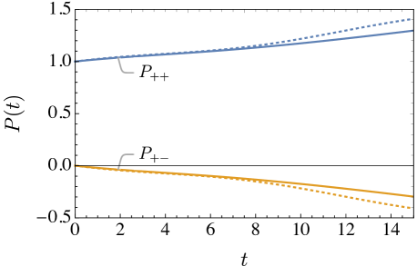
Thus, using the described method for Eq. (3.14) and assuming that and are small parameters, we series expand up to second order in and and obtain approximate analytical formulas for the transition probabilities between the and states as
| (3.33) | ||||
| (3.34) |
whose numerical results are shown as functions of time and plotted as dotted curves in the left panel of Fig. 1. It is important to note that and are not small parameters in all relevant physical situations. Thus, the validity of this approximation only holds for two-level quantum systems in which it can be argued that (i) dissipative effects, described by , are small and (ii) the diagonal elements of the Hamiltonian in Eq. (2.1) are nearly equal, quantified by . For a two-level quantum system that fulfill these two criteria, the approximation is certainly valid. In our numerical calculations, the parameter values , , , are chosen, i.e. is indeed small and is not large. One can observe that the approximate analytical results are well consistent with the exact numerical ones (see solid curves) for , but significant deviations show up for . This can be ascribed to the secular factors appearing in the series expansions, such as , which will no longer be small for large values of . In addition, and they are larger than one and increase with , while and they turn out to be negative. However, vanishes in the limit of , implying the absence of the Lindblad term. This should be the case, since there are no transitions between the and states for the PT-symmetric Hamiltonian. Furthermore, one can observe that the transition probabilities between the and states sum up to unity, i.e. , which they must in order for conservation of probability to hold. The term [and also the term ] is basically a measure of dissipative effects between the and states and also a consequence of the non-trivial metric used. Thus, in the presence of dissipative effects, the individual transition probabilities between the and states in Eqs. (3.33) and (3.34) are not restricted to values between 0 and 1, and therefore, it is not possible to consider a given state and determine its transition probabilities to itself or to the other state, whereas this is true for the conservation of probability, which is physical, i.e. there is no probability disappearing from the total two-level system (read: both of the two states). However, if the dissipative effects are turned off, i.e. , then and , and the individual transition probabilities between the and states will be restricted to either 0 or 1.
 |
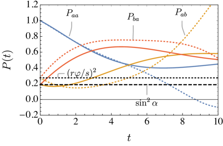 |
For the transition probabilities between the and states, we can also derive approximate analytical formulas and obtain
| (3.35) | ||||
| (3.36) |
where is found in Eq. (3.35) and the upper and lower signs in Eq. (3.36) refer to and , respectively. Both approximate analytical (dotted curves) and exact numerical (solid curves) results of these transition probabilities are presented in the right panel of Fig. 1. Three important observations can be made. First, at the initial time , one can see from Eq. (3.35) that , which is exactly the same as the numerical result. For , the initial generalized density matrices have been given in Eq. (3.21), and thus, the survival probabilities can be calculated as and . For , there is an excellent agreement between analytical and numerical results of . Second, from Eq. (3.36), we can find , which is displayed as the dotted horizontal line in the right panel of Fig. 1. However, comparing the solid and dotted curves for , one can notice that there is a sizable discrepancy between exact numerical and approximate analytical results, even at the initial time . With the help of Eq. (3.24), we can obtain and , which are shown as the dashed horizontal line in the right panel of Fig. 1. Note that approaches only if is small, which is not the situation in Fig. 1. Third, and most importantly, in contrast to the individual transition probabilities between the and states, the individual transition probabilities between the and states are always restricted to values between 0 and 1 using the exact numerical results and when the approximate analytical results hold. However, on the other hand, conservation of probability does not hold for the transition probabilities between the and states at all times , which is an effect of the non-trivial metric (). Using Eqs. (3.35) and (3.36), we find that
| (3.37) | ||||
| (3.38) |
In conclusion, for the and states, conservation of probability holds for the transition probabilities, whereas for the and states, the individual transition probabilities are restricted to values between 0 and 1. Thus, the mixing between the two different eigenbases determines which of the two bases that leads to a proper physical description of the transition probabilities of the two-level system in a given situation. If the mixing is trivial, i.e. , then the two eigenbases coincide and there is only one physical basis (and only one set of physical states). Finally, in order to solve the problem of probability non-conservation for the transition probabilities between the and states, one may renormalize the individual transition probabilities for the and states and remove the effect of the non-trivial metric in a proper way, as advocated in Ref. [48].
3.2.2 Specific Examples with
After presenting the approximate analytical formulas for the transition probabilities in the general case, we investigate some specific examples with both analytical and numerical results, and explain the main features of the dissipative effects induced by the Lindblad term.
-
1.
Two-flavor neutrino oscillations. This is a simple example of a Hermitian Hamiltonian (with a trivial metric ) that has been extensively discussed in the literature [8]. In this case, the Hamiltonian and the Lindblad equation can be written as
(3.39) implying that is constant. Note that has been given in “mass” basis with , where and are the two neutrino masses and is the neutrino energy. The structure of relates components , , and of the density matrix and the time evolution is governed by , since . As a consequence, the trace of the density matrix is equal to , which means that . We find the transition probabilities for the “mass” and “flavor” states as
(3.40) (3.41) (3.42) (3.43) where . The formulas for and should be compared to the ones in Ref. [8]. In the limit (i.e. without dissipative effects), we have and , whereas and , which are the ordinary formulas for two-flavor neutrino oscillations. Furthermore, for large values of , all transition probabilities will average to 1/2. In Fig. 2, we show the formulas for the two-flavor neutrino oscillation case with a specific choice for the parameter values (, , and ), which are not necessarily realistic and close to values supported by neutrino experiments. We note that both the transition probabilities for the “mass” and “flavor” states are damped by .

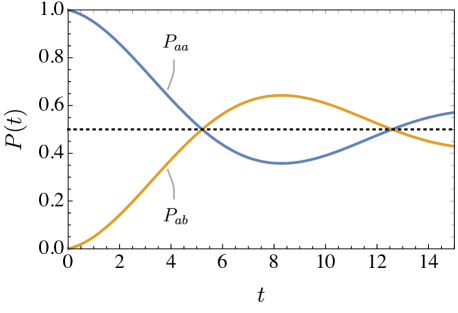
Figure 2: Two-flavor neutrino oscillations. Left: Transition probabilities for “mass” states. Right: Transition probabilities for “flavor” states. Parameter values: , , , . -
2.
PT-symmetric non-Hermitian Hamiltonian without Lindblad term. This case has been discussed in Ref. [48] without implementing the density matrix formalism. In this case, the Hamiltonian is non-Hermitian and the metric is then non-trivial. The Hamiltonian and the “Lindblad equation” (actually the Liouville–von Neumann equation) for the generalized density matrix read
(3.44) where is exactly the same as in Eq. (2.1) with . Since the metric is non-trivial, should be used and the time evolution is governed by . The structure of relates components , , and of the generalized density matrix, and thus, the trace of the generalized density matrix is equal to , which means that . For the transition probabilities between the and states, the present case reproduces Eqs. (2.24)–(2.27) in Ref. [48]. However, in order for these transition probabilities to be restricted between 0 and 1, the normalized generalized density matrix must be used after mixing with , since the completeness relation changes due to the metric being non-trivial. Thus, we obtain the transition probabilities for the and states and the and states as
(3.45) (3.46) (3.47) (3.48) (3.49) where and are defined as in Ref. [48]. It should be noted that , whereas , which is an effect of the non-trivial metric. In Fig. 3, we present the transition probabilities for the and states, since the ones for the and states are trivial. We have exactly reproduced the results in Ref. [48], when they are properly normalized. As one can observe from Fig. 3, the transition probabilities oscillate with respect to time , and no dissipative effects are found due to the absence of Lindblad operators.
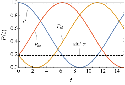
Figure 3: Transition probabilities for and states in the case of a PT-symmetric non-Hermitian Hamiltonian without Lindblad term. Parameter values: , , , , . -
3.
PT-symmetric non-Hermitian Hamiltonian with Lindblad operator but with . In this case, the Hamiltonian and the Lindblad equation for the generalized density matrix are summarized as
(3.50) where the non-Hermitian Hamiltonian is a complex diagonal matrix, and this case has a trivial metric. Since relates only the components , , and of the generalized density matrix, the trace of is equal to , which means that . In addition, the mixing matrix is trivial, since the Hamiltonian is diagonal (although complex). Hence, the and states are identical to the and states. Notice that the eigenvectors are and and that the general formulas for the eigenvectors, i.e. Eq. (2.2), cannot be used, since . The transition probabilities for both the and states and the and states are given by
(3.51) (3.52) where the Lindblad parameter brings in dissipative effects. In the large time limit , all transition probabilities approach , indicating the complete loss of quantum coherence. In Fig. 4, choosing the value of the Lindblad parameter , we display the transition probabilities, where one can clearly observe the effect of damping.

Figure 4: Transition probabilities for and states and and states in the case of a PT-symmetric non-Hermitian Hamiltonian with Lindblad term but with . Parameter value: . In order to have mixing, one can introduce an arbitrary rotation (see e.g. Ref. [11]), but it is not necessary. In the case of mixing, we find the following formulas for the transition probabilities
(3.53) (3.54) where . It turns out that all transition probabilities in Eqs. (3.51)–(3.54) are independent of both and , except from the transition probabilities in Eqs. (3.53) and (3.54) with an arbitrary rotation by the mixing angle , i.e. and . Obviously, the transition probabilities in Eqs. (3.53) and (3.54) will reduce to those without mixing in Eqs. (3.51) and (3.52) by setting .
-
4.
PT-symmetric (non-)Hermitian Hamiltonian with Lindblad operator but with . In this case, the Hamiltonian is a real off-diagonal matrix and actually Hermitian, i.e. , so the Lindblad equation for the ordinary density matrix and that for the generalized density matrix are the same. Namely, the metric is trivial . More explicitly, we have
(3.55) where the ordinary density matrix is used. It is worthwhile to point out that even the normalized density matrix is applicable, since it is reduced to the ordinary density matrix when the Hamiltonian is Hermitian, implying that and thus in Eq. (2.15). The structure of is effectively a matrix and relates only components and of the density matrix. This means that , since the trace of the density matrix should be normalized to 1. In this case, we have the transition probabilities
(3.56) (3.57) (3.58) (3.59) Note that there is no damping in the formulas for and , i.e. there is no effect of the Lindblad operator for these transition probabilities. Therefore, in Fig. 5, we plot the transition probabilities only for the and states, where the parameter values and have been chosen.
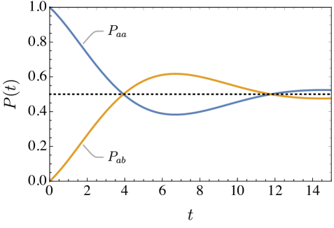
Figure 5: Transition probabilities for and states in the case of a PT-symmetric (non-)Hermitian Hamiltonian with Lindblad term but with . Parameter values: , . -
5.
Numerical example of a PT-symmetric non-Hermitian Hamiltonian with Lindblad operator. This is the most non-trivial example with all relevant parameters being non-zero. The Hamiltonian and the Lindblad equation for the generalized density matrix are
(3.60) where , , , and are adopted for numerical computations. This case has a non-Hermitian Hamiltonian and a non-trivial metric. Therefore, the generalized density matrix should be used. The structure of relates components , , and of the generalized density matrix, and thus, the trace of the generalized density matrix is equal to , which means that . However, in order for the transition probabilities to be restricted between 0 and 1, the normalized generalized density matrix must be used after mixing with , since the completeness relation changes due to the metric being non-trivial. In Fig. 6, we present the exact numerical results of the transition probabilities for the and states. Note that these transition probabilities are, of course, the same as those presented with solid curves in the right panel in Fig. 1, since we use the same parameter values.
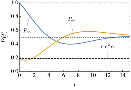
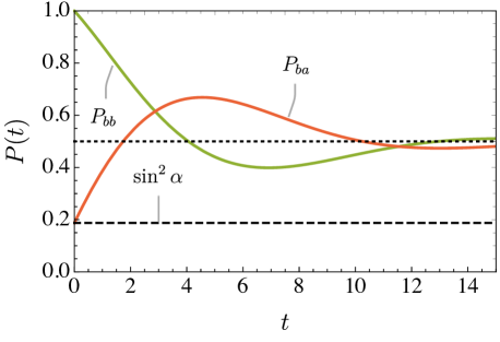
Figure 6: Numerical example of a PT-symmetric non-Hermitian Hamiltonian with Lindblad term. Transition probabilities for and states. Left: and . Right: and . Parameter values: , , , .
3.3 The Lindblad Term with
3.3.1 General Discussion
Let us investigate the case for which the structure of the Lindblad operator is changed from being described by the assumption that the Lindblad parameter to a different assumption that , which means that the other Lindblad parameters are and . Denoting the only non-zero Lindblad parameter by , we have . The explicit expression for has been given in Eq. (3.15).
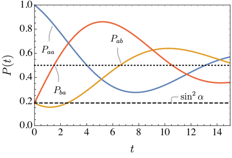
In comparison to the case , the case turns out to be much easier to handle computationally with the method described in Subsec. 3.2. In fact, in the case , all transition probabilities can be computed as simple closed-form expressions. Using the described method, we first derive exact formulas for the transition probabilities between the and states and obtain
| (3.61) | ||||
| (3.62) |
where the Lindblad parameter , causing the damping of the transition probabilities as shown in the left panel of Fig. 7. For our numerical computations, we choose , , , and . In the large time limit , all transition probabilities for the and states approach .
 |
 |
Next, we proceed to the transition probabilities between the and states. The survival probabilities are found to be
| (3.63) |
whereas the transition probabilities are given by
| (3.64) | ||||
| (3.65) |
where . It should be noted that , whereas (in general), which is an effect of the non-trivial metric. Only if or , then , which means that or . However, in the limit , it holds that . Thus, for large , probability is conserved, i.e. and . In the right panel of Fig. 7, we present the transition probabilities for the and states given by Eqs. (3.63)–(3.65), using the parameter values , , , and . The difference between and can be easily calculated as
| (3.66) |
which turns out to be an oscillatory sine function with a damping factor and vanishes in the limits of and . Compare the discussion on Eqs. (3.37) and (3.38) for the case .
3.3.2 Specific Examples with
Although it is possible to obtain exact analytical results for the Lindblad operator with , we briefly discuss a few specific examples with the same values of the relevant parameters as in the case with . Such comparative investigation should be helpful for us to understand the similarity and difference between these two cases.
-
1.
Two-flavor neutrino oscillations. In this case, we obtain the transition probabilities
(3.67) (3.68) (3.69) (3.70) where . In comparison to special case 1 for , the signs of the Lindblad parameters in front of the terms are opposite due to different positions of the Lindblad parameters in and , respectively. At all times , conservation of probability holds for both sets of transition probabilities, i.e. , and , . The formulas for and should be compared with the ones in Ref. [8]. In Fig. 8, we plot the formulas for the transition probabilities in the two-flavor neutrino oscillation case with a specific choice for the parameter values , , and , and for which one can find .
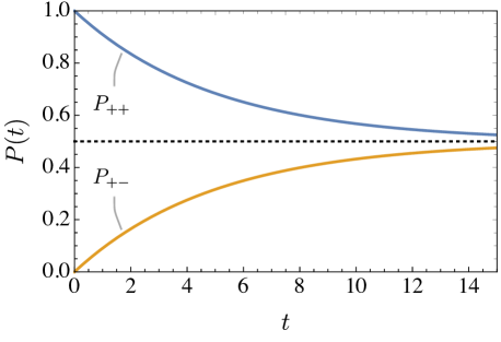
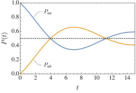
Figure 8: Two-flavor neutrino oscillations. Left: Transition probabilities for “mass” states. Right: Transition probabilities for “flavor” states. Parameter values: , , , . - 2.
-
3.
Special case . This case produces similar results as in special case 3 for , namely
(3.71) (3.72) for the transition probabilities. As mentioned in special case 3 for , the Hamiltonian is diagonal, and thus, the and states and the and states coincide with each other, implying no mixing at all. If one introduces an arbitrary rotation by the angle , the transition probabilities for the new and states are
(3.73) (3.74) where . However, compared to the counterparts in special case 3 for , the signs of the Lindblad parameters in front of the terms are opposite due to different positions of the Lindblad parameters in and , respectively. At all times , conservation of probability holds for all three sets of transition probabilities, i.e. , , , , and , . In Fig. 9, we display the transition probabilities for the and states and the and states, which are the same as those in Fig. 4.
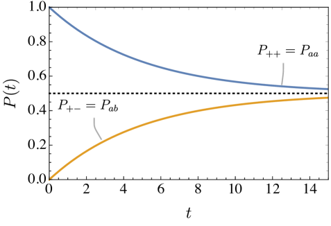
Figure 9: Special case for . Transition probabilities for and states and and states. Parameter value: . -
4.
Special case . Inserting into Eqs. (3.61)–(3.65), we find the transition probabilities
(3.75) (3.76) (3.77) (3.78) where . Note that in the limit , the non-trivial metric encoded in Eqs. (3.61)–(3.65) goes to the trivial metric . Furthermore, one can observe the differences compared to special case 4 for . At all times , conservation of probability holds for both sets of transition probabilities, i.e. , and , . In Fig. 10, we show the transition probabilities for the and states in the left panel and those for the and states in the right panel.

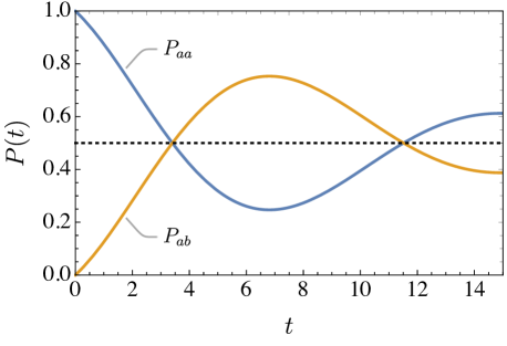
Figure 10: Special case for . Left: Transition probabilities for and states. Right: Transition probabilities for and states. Parameter values: , , .
4 Summary and Conclusions
In this work, we have developed the density matrix formalism for PT-symmetric non-Hermitian Hamiltonians, and obtained the Lindblad equation for the generalized density matrix. Moreover, we have applied this formalism with the Lindblad equation to calculate the transition probabilities of and states and those of and states in the two-level quantum system. For a general two-level quantum system, the and states should be understood as the energy eigenstates of the system in question, whereas the and states are the initially prepared quantum states as coherent superpositions of the two energy eigenstates. Our main results are summarized as follows.
First, we have performed a comparative study of the generalized density matrix and the normalized density matrix for non-Hermitian Hamiltonians . In particular, we have generalized their evolution equations to the case where the Lindblad term is present. The Lindblad equation is very useful to account for the dissipative effects due to the interaction of the quantum system in question with the external environment. In the case of generalized density matrix , where is the metric such that the pseudo-Hermiticity is fulfilled, the Lindblad equation has been first derived for the pseudo-Hermitian Hamiltonian in Refs. [39, 40]. However, we have pointed out that the condition of pseudo-Hermiticity should be imposed on the Lindblad operators , namely, . The implications of the pseudo-Hermiticity for the parameters involved in the Lindblad operators have been examined. In the case of normalized density matrix , the Liouville–von Neumann equation contains an extra term, which turns out to be quadratic in the elements of the normalized density matrix [35]. Such a non-linearity hinders the generalization to the case with the Lindblad term, which is usually derived under the assumption of linearity.
Second, based on the Lindblad equation for the generalized density matrix, we have then calculated the transition probabilities of both and states and and states in the two-level system with PT-symmetric non-Hermitian Hamiltonians. We have first proposed a new parametrization of the Lindblad operators, fulfilling pseudo-Hermiticity, and arrived at two interesting cases of either or , where and are two parameters in the Lindblad term. It is worth emphasizing that exact analytical formulas for the transition probabilities have been found in Eqs. (3.63)–(3.65) in the most general case of , where only approximate results in the case of can be obtained. Several concrete examples have then been presented, for which both analytical and numerical results of the transition probabilities are computed and compared with the existing results in the literature whenever a comparison is possible. These typical examples are instructive to clarify the main features of the Lindblad equation for PT-symmetric non-Hermitian Hamiltonians.
Finally, in the near future on the experimental side, it would be interesting to see whether the Lindblad equation derived for the generalized density matrix for PT-symmetric non-Hermitian Hamiltonians can be applied to realistic systems, such as those in optics and electronics, where the PT-symmetry has been experimentally observed. On the theoretical side, we hope to explore the general derivation of the Lindblad equation from the requirements for Markov limit, pseudo-Hermiticity, linearity, and complete positivity as in ordinary quantum mechanics.
Acknowledgments
T.O. acknowledges support by the Swedish Research Council (Vetenskapsrådet) through contract No. 2017-03934 and the KTH Royal Institute of Technology for a sabbatical period at the University of Iceland. The work of S.Z. was supported in part by the National Natural Science Foundation of China under grant No. 11775232 and No. 11835013, and by the CAS Center for Excellence in Particle Physics.
Data Availability Statement
The data that support the findings of this study are available from the corresponding author upon reasonable request.
Appendix A The Lindblad Term
In the main text, we encounter the expansions of the density matrix and the Lindblad operators in terms of Pauli matrices and the identity matrix . For reference, we collect the details of the expansions in this appendix. A general density matrix and the Lindblad operators can be expressed as follows
| (A.1) |
The Lindblad term , appearing in the evolution equations of the ordinary density matrix , the generalized one , and the normalized one , is given by
| (A.2) |
where can also be replaced by or . Nevertheless, instead of , the pseudo-Hermiticity condition holds in the latter two cases. Noticing the identity
| (A.3) |
one can write
| (A.4) | ||||
| (A.5) |
and thus, we obtain
| (A.6) |
On the other hand, we have
| (A.7) |
Inserting Eqs. (A.6) and (A.7) into Eq. (A.2), the Lindblad term can be rewritten as
| (A.8) |
which can be further simplified to
| (A.9) |
by using the identity
| (A.10) |
The final form of the Lindblad term in Eq. (A.9) has been used in our discussion in the main text.
Appendix B Four-Dimensional Representation
In the derivation of the evolution equations for the generalized density matrix and the normalized density matrix in the matrix formalism, we have to take the traces of the Lindblad equation and those together with the Pauli matrices . In this appendix, we will give some key details of calculation. For the ordinary density matrix in Hermitian quantum mechanics and in the non-Hermitian quantum mechanics under consideration, the Liouville–von Neumann equations in both cases contain similar commutators, i.e. and . Using Einstein’s summation convention, the trace of these commutators can be calculated as
| (B.1) |
whereas their trace with the Pauli matrix is
| (B.2) |
where is the three-dimensional Levi-Civita tensor. Recall that the Hamiltonian and the density matrix are expanded as and , where summation over is implied. By implementing Eqs. (B.1) and (B.2), one can immediately recast the Lindblad equation in Eq. (2.10) into the four-dimensional representation as
| (B.3) |
where the Lindblad parameters , , , , , and have been given in Eqs. (2.25)–(2.30). It is obvious that applies to the coefficient of the ordinary density matrix and also to that of the generalized density matrix .
However, for the normalized density matrix , we have to deal with , where is present as well. In the most general case, all coefficients (for ) in the expansion of are complex. Therefore, we have
| (B.4) |
Furthermore, if the trace is taken together with the Pauli matrix , then we obtain
| (B.5) |
Since there is an extra term in Eq. (2.15) in the Lindblad equation for the normalized density matrix , we should investigate the traces involving this term. Its trace can be found as
| (B.6) |
which turns out to be non-linear in (for ). When the trace is taken together with the Pauli matrix , we obtain
| (B.7) |
Thus, the four-dimensional representation of the Lindblad equation in Eq. (2.14) for the normalized density matrix becomes
| (B.8) |
where the last term is actually quadratic in (for ). Such a non-linearity seems to be in contradiction with the assumption of linearity in the derivation of the Lindblad term. Therefore, only the generalized density matrix and its Lindblad equation will be used in our calculation of transition probabilities.
Appendix C Procedure
In this work, the transition probabilities for a two-level quantum system described by a PT-symmetric non-Hermitian Hamiltonian are calculated according to the following procedure:
-
•
Given a Hamiltonian for a two-level system, construct the corresponding density matrix expressed and parametrized in terms of the identity matrix and the three Pauli matrices.
-
•
Compute the eigenvalues and construct the properly normalized eigenvectors (see Ref. [48]) and then the metric and the initial generalized density matrices.
-
•
Determine the time evolution of the density matrix for the system. The time evolution is given by the Lindblad equation for the generalized density matrix .
-
•
Transform the density matrix to a corresponding matrix with the time evolution described by a Schrödinger-like equation (with a “Hamiltonian”) for a vector with the four components of the original density matrix. Add to the “Hamiltonian” and the result is denoted , which encodes both contributions from the original Hamiltonian and the Lindblad term.
-
•
Solve the Schrödinger-like equation by matrix exponentiation of , which is denoted and leads to the time evolution for the vector of the density matrix components with the initial density matrix components as the initial condition.
-
•
Transform the vector of the density matrix components back to a density matrix.
-
•
Compute the transition probabilities between the and states by for generalized density matrices.
-
•
Construct the mixing matrix (based on the and states, known as “mass” states, see Ref. [48]), the normalized “flavor” eigenvectors (using ), i.e. the and states, and the initial “flavor” density matrices (using the normalized “flavor” eigenvectors and the metric).
-
•
Change the initial condition of the density matrix from the initial “mass” density matrices to the initial “flavor” density matrices. Note that the time evolution for the density matrix is the same in any basis, since only depends on time and the eigenvalues of , which are the same in all bases.
-
•
Compute the transition probabilities between the and states by . Note that if the metric is non-trivial, then, after mixing with (since the completeness relation changes due to the non-trivial metric), the normalized (generalized) density matrices must be used, so that the transition probabilities are restricted between 0 and 1.
References
- [1] S. Weinberg, Lectures on Quantum Mechanics, 2nd ed. (Cambridge University Press, Cambridge, UK, 2015).
- [2] G. Lindblad, “On the Generators of Quantum Dynamical Semigroups,” Commun. Math. Phys. 48, 119 (1976).
- [3] V. Gorini, A. Kossakowski and E. C. G. Sudarshan, “Completely positive dynamical semigroups of -level systems,” J. Math. Phys. 17, 821 (1976).
- [4] V. A. Franke, “On the General Form of the Dynamical Transformation of Density Matrices,” Teor. Mat. Fiz. 27, 172 (1976) [Theor. Math. Phys. 27, 406 (1976)].
- [5] R. Alicki and K. Lendi, Quantum Dynamical Semigroups and Applications (Springer, Berlin, Heidelberg, Germany, 2007).
- [6] F. Benatti and H. Narnhofer, “Entropy Behavior under Completely Positive Maps,” Lett. Math. Phys. 15, 325 (1988).
- [7] E. Lisi, A. Marrone and D. Montanino, “Probing Possible Decoherence Effects in Atmospheric Neutrino Oscillations,” Phys. Rev. Lett. 85, 1166 (2000) [arXiv:hep-ph/0002053].
- [8] F. Benatti and R. Floreanini, “Open system approach to neutrino oscillations,” JHEP 02, 032 (2000) [arXiv:hep-ph/0002221].
- [9] A. M. Gago, E. M. Santos, W. J. C. Teves and R. Zukanovich Funchal, “Quantum dissipative effects and neutrinos: Current constraints and future perspectives,” Phys. Rev. D 63, 073001 (2001) [arXiv:hep-ph/0009222].
- [10] A. M. Gago, E. M. Santos, W. J. C. Teves and R. Zukanovich Funchal, “Quest for the dynamics of conversion,” Phys. Rev. D 63, 113013 (2001) [arXiv:hep-ph/0010092].
- [11] T. Ohlsson, “Equivalence between Gaussian averaged neutrino oscillations and neutrino decoherence,” Phys. Lett. B 502, 159 (2001) [arXiv:hep-ph/0012272].
- [12] F. Benatti and R. Floreanini, “Massless neutrino oscillations,” Phys. Rev. D 64, 085015 (2001) [arXiv:hep-ph/0105303].
- [13] A. M. Gago, E. M. Santos, W. J. C. Teves and R. Zukanovich Funchal, “A study on quantum decoherence phenomena with three generations of neutrinos,” [arXiv:hep-ph/0208166].
- [14] M. M. Guzzo, P. C. de Holanda and R. L. N. Oliveira, “Quantum dissipation in a neutrino system propagating in vacuum and in matter,” Nucl. Phys. B 908, 408 (2016) [arXiv:1408.0823 [hep-ph]].
- [15] D. Boriero, D. J. Schwarz and H. Velten, “Flavour Composition and Entropy Increase of Cosmological Neutrinos after Decoherence,” Universe 5, 203 (2019) [arXiv:1704.06139 [astro-ph.CO]].
- [16] P. Coloma, J. Lopez-Pavon, I. Martinez-Soler and H. Nunokawa, “Decoherence in neutrino propagation through matter, and bounds from IceCube/DeepCore,” Eur. Phys. J. C 78, 614 (2018) [arXiv:1803.04438 [hep-ph]].
- [17] G. Balieiro Gomes, D. V. Forero, M. M. Guzzo, P. C. de Holanda and R. L. N. Oliveira, “Quantum decoherence effects in neutrino oscillations at DUNE,” Phys. Rev. D 100, 055023 (2019) [arXiv:1805.09818 [hep-ph]].
- [18] A. L. G. Gomes, R. A. Gomes and O. L. G. Peres, “Quantum decoherence and relaxation in neutrinos using long-baseline data,” [arXiv:2001.09250 [hep-ph]].
- [19] B. Kerbikov, “Lindblad and Bloch equations for conversion of a neutron into an antineutron,” Nucl. Phys. A 975, 59 (2018) [arXiv:1704.07117 [hep-ph]].
- [20] S. Weinberg, “Lindblad decoherence in atomic clocks,” Phys. Rev. A 94, 042117 (2016) [arXiv:1610.02537 [quant-ph]].
- [21] R. Salah, A. M. Farouk, A. Farouk, M. Abdel-Aty, H. Eleuch and A.-S. F. Obada, “Entanglement Control of Two-Level Atoms in Dissipative Cavities,” Appl. Sci. 10, 1510 (2020) [arXiv:1908.00776 [quant-ph]].
- [22] D. Leibfried, R. Blatt, C. Monroe and D. Wineland, “Quantum dynamics of single trapped ions,” Rev. Mod. Phys. 75, 281 (2003)
- [23] Á. Parra-López and J. Bergli, “Synchronization in two-level quantum systems,” Phys. Rev. A 101, 062104 (2020) [arXiv:1904.11763 [quant-ph]].
- [24] B. Bonnard, O. Cots, N. Shcherbakova and D. Sugny, “The energy minimization problem for two-level dissipative quantum systems,” J. Math. Phys. 51, 092705 (2010)
- [25] T. Vieillard, F. Chaussard, D. Sugny, B. Lavorel and O. Faucher, “Field-free molecular alignment of mixtures in presence of collisional relaxation,” J. Raman Spectrosc. 39, 694 (2008)
- [26] B. Bonnard, M. Chyba and D. Sugny, “Time-Minimal Control of Dissipative Two-Level Quantum Systems: The Generic Case,” IEEE Trans. Automat. Contr. 54, 2598 (2009)
- [27] R. El-Ganainy et al., “Non-Hermitian physics and PT symmetry,” Nat. Phys. 14, 11 (2018).
- [28] F. Benatti and R. Floreanini, “Complete positivity and the - system,” Phys. Lett. B 389, 100 (1996) [arXiv:hep-th/9607059].
- [29] F. Benatti and R. Floreanini, “Completely positive dynamical maps and the neutral kaon system,” Nucl. Phys. B 488, 335 (1997)
- [30] F. Benatti and R. Floreanini, “Experimental limits on complete positivity from the system,” Phys. Lett. B 401, 337 (1997) [arXiv:hep-ph/9704283].
- [31] F. Benatti and R. Floreanini, “Completely positive dynamics of correlated neutral kaons,” Nucl. Phys. B 511, 550 (1998) [arXiv:hep-ph/9711240].
- [32] R. A. Bertlmann, W. Grimus and B. C. Hiesmayr, “Open-quantum-system formulation of particle decay,” Phys. Rev. A 73, 054101 (2006) [arXiv:quant-ph/0602116].
- [33] J. Bernabéu, N. E. Mavromatos and P. Villanueva-Pérez, “Consistent probabilistic description of the neutral Kaon system,” Phys. Lett. B 724, 269 (2013) [arXiv:1208.3572 [hep-ph]].
- [34] T. D. Lee and L. Wolfenstein, “Analysis of -Noninvariant Interactions and the , System,” Phys. Rev. 138, B1490 (1965).
- [35] A. Sergi and K. G. Zloshchastiev, “Non-Hermitian Quantum Dynamics of a Two-Level System and Models of Dissipative Environments,” Int. J. Mod. Phys. B 27, 1350163 (2013) [arXiv:1207.4877 [quant-ph]].
- [36] A. Sergi and K. G. Zloshchastiev, “Time correlation functions for non-Hermitian quantum systems,” Phys. Rev. A 91, 062108 (2015) [arXiv:1412.5782 [quant-ph]].
- [37] C.-Y. Ju, A. Miranowicz, G.-Y. Chen and F. Nori, “Non-Hermitian Hamiltonians and no-go theorems in quantum information,” Phys. Rev. A 100, 062118 (2019) [arXiv:1906.08071 [quant-ph]].
- [38] A. Mostafazadeh, “Pseudo-Hermitian Representation of Quantum Mechanics,” Int. J. Geom. Meth. Mod. Phys. 07, 1191 (2010) [arXiv:0810.5643 [quant-ph]].
- [39] G. Scolarici and L. Solombrino, “Time evolution of non-Hermitian quantum systems and generalized master equations,” Czech. J. Phys. 56, 935 (2006).
- [40] G. Scolarici, “Complex Projection of Quasianti-Hermitian Quaternionic Hamiltonian Dynamics,” SIGMA 3, 088 (2007) [arXiv:0709.1198 [math-ph]].
- [41] C. M. Bender and S. Boettcher, “Real Spectra in Non-Hermitian Hamiltonians Having Symmetry,” Phys. Rev. Lett. 80, 5243 (1998) [arXiv:physics/9712001].
- [42] C. M. Bender, S. Boettcher and P. N. Meisinger, “PT-symmetric quantum mechanics,” J. Math. Phys. 40, 2201 (1999) [arXiv:quant-ph/9809072].
- [43] C. M. Bender, M. V. Berry and A. Mandilara, “Generalized PT symmetry and real spectra,” J. Phys. A 35, L467 (2002).
- [44] C. M. Bender, D. C. Brody and H. F. Jones, “Complex Extension of Quantum Mechanics,” Phys. Rev. Lett. 89, 270401 (2002) [arXiv:quant-ph/0208076].
- [45] C. M. Bender, P. N. Meisinger and Q. h. Wang, “Finite-dimensional PT-symmetric Hamiltonians,” J. Phys. A 36, 6791 (2003) [arXiv:quant-ph/0303174].
- [46] C. M. Bender, “Making sense of non-Hermitian Hamiltonians,” Rep. Prog. Phys. 70, 947 (2007) [arXiv:hep-th/0703096].
- [47] T. Ohlsson, “Non-Hermitian neutrino oscillations in matter with PT symmetric Hamiltonians,” EPL 113, 61001 (2016) [arXiv:1509.06452 [hep-ph]].
- [48] T. Ohlsson and S. Zhou, “Transition probabilities in the two-level quantum system with PT-symmetric non-Hermitian Hamiltonians,” J. Math. Phys. 61, 052104 (2020) [arXiv:1906.01567 [quant-ph]].
- [49] T. Ohlsson and S. Zhou, “Transition Probabilities for Flavor Eigenstates of Non-Hermitian Hamiltonians in the PT-Broken Phase,” [arXiv:2002.05499 [quant-ph]].
- [50] O. Cherbal and M. Drir, “Dissipative Two-Level Spin System and Geometrical Phase,” Proceedings of the Seventh International Conference on Geometry, Integrability and Quantization (Softex, Sofia, Bulgaria, 2006), 79-88
- [51] D. Sugny, C. Kontz and H. R. Jauslin, “Time-optimal control of a two-level dissipative quantum system,” Phys. Rev. A 76, 023419 (2007) [arXiv:0708.3794 [quant-ph]].
- [52] F. Kleefeld, “The construction of a general inner product in non-Hermitian quantum theory and some explanation for the nonuniqueness of the operator in quantum mechanics,” [arXiv:0906.1011 [hep-th]].
- [53] P. Pearle, “Simple derivation of the Lindblad equation,” Eur. J. Phys. 33, 805 (2012) [arXiv:1204.2016 [math-ph]].
- [54] T. Ohlsson and H. Snellman, “Three flavor neutrino oscillations in matter,” J. Math. Phys. 41, 2768 (2000); ibid. 42, 2345(E) (2001) [arXiv:hep-ph/9910546].