Transverse-Energy-Energy Correlations in Deep Inelastic Scattering
Abstract
Event shape observables have been widely used for precision QCD studies at various lepton and hadron colliders. We present the most accurate calculation of the transverse-energy-energy correlation event shape variable in deep-inelastic scattering. In the framework of soft-collinear effective theory the cross section is factorized as the convolution of the hard function, beam function, jet function and soft function in the back-to-back limit. A close connection to TMD factorization is established, as the beam function when combined with part of the soft function is identical to the conventional TMD parton distribution function, and the jet function is the second moment of the TMD fragmentation function matching coefficient. We validate our framework by comparing the obtained LO and NLO leading singular distributions to the full QCD calculations in the back-to-back limit. We report the resummed transverse-energy-energy correlation distributions up to N3LL accuracy matched with the NLO cross section for the production of a lepton and two jets. Our work provides a new way to precisely study TMD physics at the future Electron-Ion Collider.
1 Introduction
Event shape observables describe the patterns, correlations, and energy flow of hadronic final states in high energy processes. They have been widely investigated to study the various dynamical aspects of QCD in , , , and heavy-ion collisions. Event shape variables can be used to determine the strong coupling and test asymptotic freedom, to tune the nonperturbative Quantum Chromodynamics (QCD) power corrections, and to search for new physics phenomena. Furthermore, these observables can be studied with high precision theoretically and compared to experimental measurements at the future Electron-Ion Collider (EIC).
There are many efforts devoted to the study of event shape observables in deep-inelastic scattering (DIS). The next-to-leading order (NLO) QCD corrections were obtained about twenty years ago Catani:1996vz ; Graudenz:1997gv ; Nagy:2001xb . Recently, the next-to-next-to-leading order (NNLO) QCD corrections to various event shape distributions were computed in ref. Gehrmann:2019hwf . Near the infrared region resummation is required to obtain reliable predictions, which are available at next-to-leading logarithmic (NLL) level Antonelli:1999kx ; Dasgupta:2001eq ; Dasgupta:2002dc ; Dasgupta:2003iq for most event shape observables, next-to-next-to-leading logarithmic (NNLL) level for 1-jettiness Kang:2013lga and angularity Kang:2019bpl , and next-to-next-to-next-to-leading logarithmic (N3LL) level for thrust Kang:2015swk . On the experimental side, H1 and ZEUS collaborations have measured some event shape variables at HERA Adloff:1997gq ; Breitweg:1997ug ; Adloff:1999gn ; Chekanov:2002xk ; Aktas:2005tz ; Chekanov:2006hv . With more precise measurements in DIS at the future EIC, event shape observables can serve as a precision test of QCD and new probes to reveal the proton or nuclear structure.
Here, we will concentrate on the transverse-energy-energy correlation (TEEC) event shape observable in DIS. TEEC Ali:1984yp at hadronic colliders is an extension of the energy-energy correlation (EEC) Basham:1978bw variable introduced decades ago in collisions to describe the global event shape. The EEC is defined as
| (1) |
where is the energy of hadron and is the opening angle between hadrons and . New studies of EECs, which include analytical NLO calculations Dixon:2018qgp ; Luo:2019nig , NNLO in super-Yang-Mills theory Belitsky:2013xxa ; Belitsky:2013bja ; Belitsky:2013ofa ; Henn:2019gkr , all-order factorization in QCD in the back-to-back limit Moult:2018jzp , and all order structure in the collinear limit Dixon:2019uzg ; Kologlu:2019mfz ; Korchemsky:2019nzm ; Chen:2020uvt , have furthered our understanding of this observable.
At hadronic colliders, where detectors lack the typical hermeticity of detectors at machines, the event shape observable can be generalized by considering the transverse energy of the hadrons. TEEC, which is defined as
| (2) |
was investigated in refs. Ali:2012rn ; Gao:2019ojf ; Gao:2019prep . In eq. (2) is the transverse energy of hadron and is the azimuthal angle between hadrons and . The NLO QCD corrections for the TEEC observable were calculated in ref. Ali:2012rn . The works Gao:2019ojf ; Gao:2019prep investigated TEEC in the dijet limit and showed that it exhibits remarkable perturbative simplicity.
In DIS, TEEC can be generalized by considering the transverse-energy and transverse-energy correlation between the lepton and hadrons in the final state, which is first studied in this work. We define this event shape observable as follows:
| (3) |
where the sum runs over all the hadrons in the final states and is the azimuthal angle between final state lepton and hadron . Note that there is no QCD collinear singularity () along the outgoing lepton’s momentum in DIS, for which one needs to perform the resummation at hadron colliders and in annihilation Dixon:2019uzg . As we will show below, resummed predictions in the back-to-back limit () can be obtained to high accuracy and the distribution in the whole range can be reliably calculated. One of the advantages of EEC/TEEC is that the contribution from soft radiation is suppressed as it carries parametrically small energy. Therefore, the hadronization effects are expected to be small in comparison to other event shape observables. TEEC in DIS can be used to determine the strong coupling precisely similar to analysis in refs. Catani:1996vz ; Graudenz:1997gv ; Nagy:2001xb and to study the nuclear dynamic as in ref. Kang:2013lga . Additionally it is also feasible to study transverse-momentum dependent (TMD) physics using TEEC in DIS.
In this paper, we present our study of TEEC in the DIS process. Similar to EEC Moult:2018jzp in collisions and TEEC Gao:2019ojf in hadronic collisions, the cross section for this observable in the back-to-back limit can be factorized as the convolution of the hard function, beam function, jet function, and soft function using the frameworks of soft-collinear effective theory (SCET) Bauer:2001yt ; Bauer:2001ct ; Bauer:2000yr ; Bauer:2000ew ; Beneke:2002ph . This approach is similar to a 1-dimension TMD factorization and is, thus, closely related to TMD physics. The beam functions are identical to the TMD parton distribution functions (PDFs) and the jet function is the second moment of the matching coefficients of the TMD fragmentation functions. For details see refs. Moult:2018jzp ; Luo:2019hmp ; Luo:2019bmw . Furthermore, the factorization formalism is also similar to the usual TMD factorization, for example see the work Gutierrez-Reyes:2019vbx for N3LL jet distribution. The non-trivial LO and NLO QCD distributions of the TEEC observable are reproduced by the leading power SCET in the back-to-back limit, which validates our formalism. Resummation can be achieved by evolving each component of the factorized expression from its intrinsic scale to a suitably chosen common scale. The main goal of our work is to present the most precise TEEC predictions in DIS at N3LL+NLO. The effects of the nonperturbative physics are also discussed. Since there is no collinear singularity, we are able to provide the N3LL+NLO distribution in the complete range of . The perturbative behavior of this observable is under good theoretical control in QCD, which can be further improved if one can match the resummation with NNLO corrections. Consequently, it can be used to study the non-perturbative physics in a precise quantitative manner.
The rest of this paper is organized as follows. In the next section the factorization formalism for the TEEC observable is present. The hard function, beam function, jet function, and soft function are discussed. In Section 3 we investigate the hadronization effect using Pythia8. We further verify the factorization formula by comparing the LO and NLO singular distribution with the full QCD ones. The N3LL and N3LL+NLO predictions are also present. Finally, we conclude in Section 4. The RG equations and anomalous dimensions are present in Appendix A.
2 Theoretical formalism
The underlying partonic Born process considered in this work is
| (4) |
The first order non-trivial contribution to TEEC begins from one order higher. In the back-to-back limit, the TEEC cross section is defined as
| (5) |
where is the transverse momentum of the outgoing lepton. We define the momenta of the event in the plane, i.e. at LO the components of all the momenta along -direction are zero. In the back-to-back limit it is convenient to introduce the variable , related to the non-zero momentum balance along -direction of the event due to soft and/or collinear radiations. It can be written as
| (6) |
where is the -momentum of the soft radiation and is the momentum fraction of the hadron relative to the jet. The soft radiation contributes through the recoil to the energetic collinear partons. Similar to the case of EEC in electron-position collisions or TEEC at hadronic collisions, the cross section in the back-to-back limit is factorized into the convolution of a hard function, beam function, soft function, and jet function. Specifically, up to leading power in SCET the cross section can be written as
| (7) |
where , is the conjugate variable to , is the invariant mass of the virtual photon, and . Four-vectors and represent the momentum directions of the momenta and , respectively. and are the energies of and . is rapidity scale associated with the rapidity regulator for which we adopt the exponential regulator introduced in ref. Li:2016axz .
, which describe the contribution from collinear radiation in the initial state, are the same as the usual TMD beam functions. The operator definition for the beam function in SCET is
| (8) |
with , where is the collinear quark field and is the path-ordered collinear Wilson line . In the operator definition, we suppress the arguments of kinematics and scales. The TMD beam functions have been calculated up to three loops for quark beam functions and two loops for gluon beam functions Gehrmann:2012ze ; Gehrmann:2014yya ; Luebbert:2016itl ; Echevarria:2016scs ; Luo:2019hmp ; Luo:2019bmw ; Luo:2019szz .
The jet functions are defined as the second Mellin moment of the matching coefficients of the TMD fragmentation function Echevarria:2016scs ; Echevarria:2015usa ; Luo:2019hmp ; Luo:2019bmw . The explicit expression up to two loops for the jet functions can be found in refs. Luo:2019hmp ; Luo:2019bmw .
The operator definition for the soft function is
| (9) |
where and correspond to an incoming quark and an outgoing quark, respectively. The explicit expressions of and are
| (10) |
We suppress the arguments of kinematics and scales in the operator definition. The soft function for TEEC in DIS can be written in terms of the soft function in EEC in collisions, which can be written as
| (11) |
where is the soft function for EEC. In the above and with . is identical to TMD soft function Moult:2018jzp . Up to three loops the expression for the soft function can be found in refs. Li:2016ctv .
The hard function encodes the short-distance physics, which is the matching coefficient from full QCD onto SCET. The analytical expression of up to NNLO is given in ref. Becher:2006mr and the one at three-loop level can be obtained from the quark form factor, as shown in refs. Baikov:2009bg ; Gehrmann:2010ue .
The renormalization group (RG) equations and anomalous dimensions needed for our calculation are given in Appendix A. With all the components and their RG equations available, we can achieve precision predictions for this observable up to N3LL. The resummed cross section is obtained by evolving the hard function from to and the soft function from to . It can be written as
| (12) |
where and are the anomalous dimensions of the hard and soft functions, and is the rapidity anomalous dimension of the soft function.
The prediction away from the back-to-back limit is obtained through matching the resummed calculations with the fixed-order ones, which can be written as
| (13) |
The singular distribution is the fixed-order prediction from eq. (2) in the leading power of SCET, which captures the singular behavior of the QCD fixed-order predictions in the leading power in the back-to-back limit.
3 Numerical results
We will present numerical predictions with enter-of-mass energy GeV, corresponding to beam energies 20 (lepton) GeV250 (proton) GeV, typical for the future EIC Aschenauer:2014cki . We also consider enter-of-mass energy GeV, corresponding to beam energies 27.5 GeV920 GeV at HERA. We select events with constraints on the transverse momentum of the outgoing lepton GeV and GeV for 141 GeV and 318 GeV electron-proton collisions, respectively. All calculations are performed using PDF4LHC15_nnlo_mc PDF sets Butterworth:2015oua ; Dulat:2015mca ; Harland-Lang:2014zoa ; Ball:2014uwa and the associated strong coupling provided by Lhapdf6 Buckley:2014ana .
3.1 Pythia Simulation
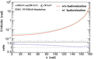
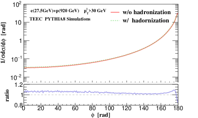
To assess the effects of hadronization on the TEEC observable we start with Pythia8 Sjostrand:2007gs ; Sjostrand:2014zea simulations. Figure 1 shows the predictions for normalized TEEC with and without hadronization in 141 Gev (left) and 318 GeV (right) collisions. The lepton is selected with a finite transverse momentum in the final state and there is no divergence in the usual collinear limit (). The cross section is dominated by the back-to-back region, where there are collinear and/or soft singularities in fixed-order calculations. As shown in Fig. 1, the hadronization effects are more important in GeV collisions since the tagged lepton is of a smaller . The corrections themselves are about 20 to 35 percent for small and large . For GeV collisions the hadronization effects are a few percent for small and about 15% in the back-to-back region. In comparison to other event shape observables, as can be seen in the simulations in ref. Gehrmann:2019hwf , the overall hadronization effects are much smaller. The reason behind this observation is that the soft particle contribution is suppressed by the energy in the TEEC. Therefore, the predictions for the TEEC observable can be significantly improved through high order calculations in perturbative QCD. In this section we will show that N3LL TEEC in the back-back limit is under very good control after resummation and the nonperturbative effects are investigated. In the future the distributions can be further improved with NNLO calculations. Subsequently, the observable can be used to test perturbative QCD and measure the QCD coupling in a unique way.
3.2 Fixed-order results
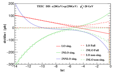
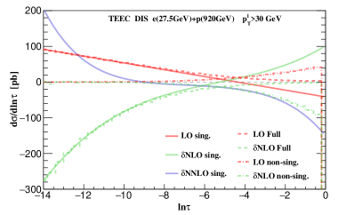
We now move on to the core calculations in our work on TEEC in DIS. In Fig. 2 we present the comparison of the leading singular distributions from SCET to full QCD calculations. Figure 2 also shows the non-singular contributions which are defined as the differences between the full QCD and the singular calculations. With the known components in eq. (2) up to two loops, the LO and NLO singular distributions are present with solid orange and solid green lines. With three-loop anomalous dimensions the singular distributions are calculated up to NNLO in QCD and are shown as the solid blue lines. The singular distributions oscillate between and from LO to NNLO when . The full LO and NLO results for two jet production in DIS are calculated making use of Nlojet++ Nagy:2001xb ; Nagy:2005gn and are denoted by dashed lines. Finally, the dash-dotted lines stand for the non-singular distributions. The renormalization and factorization scales are set to be . The LO and NLO singular distributions from SCET perfectly reproduce the full QCD results in the back-to-back limit, which provides a solid check of our factorization formalism. In the range , the factorization formula does not work well and there are large power corrections, as expected. For small the logarithmic structures in the singular distributions needed to be resummed to all orders in to obtain stable predictions.
3.3 Resummed predictions
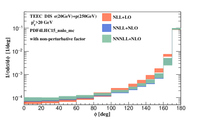
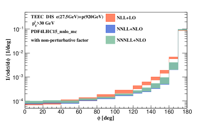
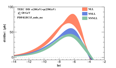
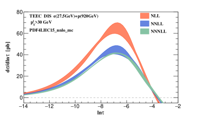
We set the default scales in our calculation to , . The scale uncertainties are defined as the quadratic sum over the results when we vary , , , and independently by a factor of two around their default values. To avoid Landau pole we use the prescription Collins:1981va and define . We further define and set GeV-1. For completeness, we varied the nonperturbative parameter GeV GeV-1. We found that the dependence on of the resummed distributions is very small.
Figure 3 presents the resummed predictions at NLL, NNLL, and N3LL accuracy in the back-to-back limit with scale uncertainties. We find very good perturbative convergence. There is about 30% suppression in the peak region from NLL to NNLL, while it is about 5-6% from NNLL to N3LL. The scale uncertainty of the N3LL result is larger for 141 GeV collisions, and is around 12% near the peak. For 318 GeV collisions the uncertainty is only about 2%. The factorization formula gives more accurate predictions at GeV due to larger scale hierarchy. In both cases the uncertainties are significantly improved order-by-order. The resummed distributions turn negative when where the effective theory becomes invalid.
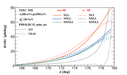
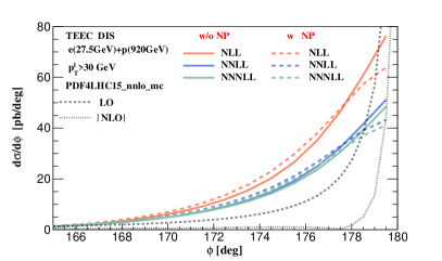
In general the nonperturbative (NP) corrections can be important in the infrared region. For EEC in collisions, the work Dokshitzer:1999sh investigated the nonperturbative effects in detail using and a power corrections scheme. However, we use a different approach, the prescription, commonly found in hadron collider phenomenology to deal with the Landau pole. The nonperturbative effects for TEEC in DIS are related to initial state PDFs, or beam functions, which is different in comparison with the case of EEC. In this work choose the non-perturbative model used in resummation with parameters obtained through fitting data from refs. Su:2014wpa ; Prokudin:2015ysa . The nonperturbative effects are included by a multiplicative factor in eq. (2)
| (14) |
with GeV. Figure 4 shows the effect of the nonperturbative factor, where the solid and dashed lines are the predictions without and with the NP factor, respectively. The nonperturbative factor suppresses the cross section for where low-energy physics is important. The nonperturbative effects are larger in 141 GeV collisions when compared to those in 318 GeV collisions because the corresponding cross section in 141 GeV collisions has a smaller intrinsic scale. Figure 4 also includes the and 111The NLO cross section turns negative when is very close to 180o., which are represented by gray dashed and dotted lines. The fixed-order predictions are divergent when as expected. Resummation improves these predictions considerably.
Eq. (14) is not the only possible form of nonperturbative corrections. For example, for EEC, the work Dokshitzer:1999sh considered both a quadratic and a linear contributions in the impact parameter . The latter can arise from correlations between quarks and soft gluons emitted at the scale of order and can give a dominant contribution to the NP effects. A study along those lines in the future can help us better understand the interplay between the perturbative and non-perturbative corrections in the back-to-back region.
The results for the normalized TEEC distributions are shown in Fig. 5, where the nonperturbative factor from eq. (14) is also implemented. The matching region is chosen to be and for the distributions are generated by fixed-order calculations. The fixed-order predictions are calculated with with . In the back-to-back limit, the predictions are significantly improved. For the second to last bin in Fig. 5 where or , the non-singular contributions are large, which is consistent with Fig. 2 and Fig. 3. The scale uncertainties are dominated by the non-singular terms. The scale uncertainties for the normalized distributions at NNLL+NLO and N3LL+NLO are dominated by the NLO calculations away from the back-to-back region. Because of accidental cancellation of the scale dependence for the normalized TEEC distributions at LO, it seems that the NLO QCD corrections do not reduce the scale uncertainties. However, as documented in ref. Gehrmann:2019hwf , the NNLO QCD corrections are expected to reduce the scale dependence of event shape observables significantly. Therefore, we expect that matching with NNLO QCD calculations will further reduce the scale uncertainties, but is beyond the scope of this paper. The resummation improves the prediction significantly for . There is a small difference for between NNLL+NLO and N3LL+NLO because in a normalized distribution changes in a few bins will affect the distribution in the whole plotted range.
4 Conclusion
In this paper, we carried out the first study on TEEC in DIS. In the back-to-back limit the TEEC cross section can be factorized into the product of the hard function, beam function, jet function, and soft function in position space – closely related to the ordinary TMD physics. We validated the formalism by comparing our LO and NLO singular distributions to the full QCD calculations in the back-to-back limit. The NNLO singular distribution is also provided as a future cross-check of the NNLO cross section for 2jet. The resummed distributions were obtained through solving the RG equations for each component. We found very good perturbative convergence and the scale uncertainties were significantly reduced order-by-order. The nonperturbative effects were assessed using Pythia simulations and a nonperturbative model widely used in resummation. Importantly, we presented the first theoretical prediction for distributions at N3LL+NLO accuracy. In the future it will be interesting to consider on the perturbative side matching to an NNLO fixed order calculation Gehrmann:2019hwf . On the nonperturbative side one can explore corrections that arise from quark-gluon correlations and might have a different functional form Dokshitzer:1999sh than the ones included here.
The EEC/TEEC event shape observables can be studied in , and collisions, which provides a way to test the universality of QCD factorization in different colliding systems. These observables can also be used to study TMD physics, which is one of the most important goals of the EIC. Finally, we remark that TEEC can also be used to shed light on the interaction between partons and a QCD medium in electron-ion () or ion-ion () collisions. Ongoing theoretical and experimental design efforts aim to elucidate the physics opportunities with hadron and jet modification at the EIC and, very importantly, to ensure that the detectors at this future facility have the capabilities to perform the necessary measurements, see e.g. ref. Li:2020sru .
As our calculations rely on the SCET framework, a natural choice to address TEEC in collisions is the extension of the effective theory approach to include the interactions between partons and the background QCD medium mediated by Glauber gluons. Soft collinear effective theory with Glauber gluon interactions has provided a mean to evaluate the contribution in-medium parton showers Ovanesyan:2011xy ; Kang:2016ofv to a variety of observables in reactions with nuclei. The most recent examples include the modification of jet cross sections and jet substructure ranging from the jet splitting functions to the jet charge Li:2018xuv ; Li:2017wwc ; Li:2019dre . To obtain predictions for the TEEC event shape observable in DIS on nuclei will require a computation of the contributions from parton branching in strongly-interacting matter to the terms in the master factorization formula. This deserves a separate paper and will be one of our future goals.
Acknowledgement
We thank F. Yuan and H.X. Zhu for the collaboration at the early stage of the project. H.T. Li was supported by the Los Alamos National Laboratory LDRD program. I. Vitev was supported by the U.S. Department of Energy under Contract No. DE-AC52-06NA25396 and by the LANL LDRD program. Y.J. Zhu was supported in part by NSFC under contract No. 11975200.
Appendix A Anomalous dimensions
The RG equation of the hard function is
| (15) |
up to four loops and up to three loops were collected in ref. Becher:2019avh and references therein. The RG equation of the beam/jet function reads
| (16) |
where represents the beam function or the jet function . is the energy of parton . The RG equation of the soft function is given by
| (17) |
The expressions for up to three loops can be found in refs. Li:2016ctv ; Moult:2018jzp . Additionally we have , which can be derived from according to the scale invariance of the cross sections. Note that
| (18) |
with .
The rapidity evolution equation of the beam/jet function reads
| (19) |
Similarly, the rapidity evolution equation of the soft function is given by
| (20) |
where can be found in refs. Li:2016ctv ; Moult:2018jzp . The cross section is independent of , which leads to the constraint
| (21) |
References
- (1) S. Catani and M. H. Seymour, A General algorithm for calculating jet cross-sections in NLO QCD, Nucl. Phys. B485 (1997) 291–419, [hep-ph/9605323].
- (2) D. Graudenz, Disaster++: Version 1.0, hep-ph/9710244.
- (3) Z. Nagy and Z. Trocsanyi, Multijet cross-sections in deep inelastic scattering at next-to-leading order, Phys. Rev. Lett. 87 (2001) 082001, [hep-ph/0104315].
- (4) T. Gehrmann, A. Huss, J. Mo and J. Niehues, Second-order QCD corrections to event shape distributions in deep inelastic scattering, Eur. Phys. J. C 79 (2019) 1022, [1909.02760].
- (5) V. Antonelli, M. Dasgupta and G. P. Salam, Resummation of thrust distributions in DIS, JHEP 02 (2000) 001, [hep-ph/9912488].
- (6) M. Dasgupta and G. P. Salam, Resummation of the jet broadening in DIS, Eur. Phys. J. C24 (2002) 213–236, [hep-ph/0110213].
- (7) M. Dasgupta and G. P. Salam, Resummed event shape variables in DIS, JHEP 08 (2002) 032, [hep-ph/0208073].
- (8) M. Dasgupta and G. P. Salam, Event shapes in e+ e- annihilation and deep inelastic scattering, J. Phys. G30 (2004) R143, [hep-ph/0312283].
- (9) Z.-B. Kang, X. Liu and S. Mantry, 1-jettiness DIS event shape: NNLL+NLO results, Phys. Rev. D90 (2014) 014041, [1312.0301].
- (10) D. Kang and T. Maji, Toward precision jet event shape for future Electron-Ion Collider, in Light Cone 2019, 12, 2019. 1912.10656.
- (11) D. Kang, C. Lee and I. W. Stewart, DIS Event Shape at N3LL, PoS DIS2015 (2015) 142.
- (12) H1 collaboration, C. Adloff et al., Measurement of event shape variables in deep inelastic e p scattering, Phys. Lett. B406 (1997) 256–270, [hep-ex/9706002].
- (13) ZEUS collaboration, J. Breitweg et al., Event shape analysis of deep inelastic scattering events with a large rapidity gap at HERA, Phys. Lett. B421 (1998) 368–384, [hep-ex/9710027].
- (14) H1 collaboration, C. Adloff et al., Investigation of power corrections to event shape variables measured in deep inelastic scattering, Eur. Phys. J. C14 (2000) 255–269, [hep-ex/9912052].
- (15) ZEUS collaboration, S. Chekanov et al., Measurement of event shapes in deep inelastic scattering at HERA, Eur. Phys. J. C27 (2003) 531–545, [hep-ex/0211040].
- (16) H1 collaboration, A. Aktas et al., Measurement of event shape variables in deep-inelastic scattering at HERA, Eur. Phys. J. C46 (2006) 343–356, [hep-ex/0512014].
- (17) ZEUS collaboration, S. Chekanov et al., Event shapes in deep inelastic scattering at HERA, Nucl. Phys. B767 (2007) 1–28, [hep-ex/0604032].
- (18) A. Ali, E. Pietarinen and W. Stirling, Transverse Energy-energy Correlations: A Test of Perturbative QCD for the Proton - Anti-proton Collider, Phys. Lett. B 141 (1984) 447–454.
- (19) C. Basham, L. S. Brown, S. D. Ellis and S. T. Love, Energy Correlations in electron - Positron Annihilation: Testing QCD, Phys. Rev. Lett. 41 (1978) 1585.
- (20) L. J. Dixon, M.-X. Luo, V. Shtabovenko, T.-Z. Yang and H. X. Zhu, Analytical Computation of Energy-Energy Correlation at Next-to-Leading Order in QCD, Phys. Rev. Lett. 120 (2018) 102001, [1801.03219].
- (21) M.-X. Luo, V. Shtabovenko, T.-Z. Yang and H. X. Zhu, Analytic Next-To-Leading Order Calculation of Energy-Energy Correlation in Gluon-Initiated Higgs Decays, JHEP 06 (2019) 037, [1903.07277].
- (22) A. V. Belitsky, S. Hohenegger, G. P. Korchemsky, E. Sokatchev and A. Zhiboedov, From correlation functions to event shapes, Nucl. Phys. B884 (2014) 305–343, [1309.0769].
- (23) A. V. Belitsky, S. Hohenegger, G. P. Korchemsky, E. Sokatchev and A. Zhiboedov, Event shapes in super-Yang-Mills theory, Nucl. Phys. B884 (2014) 206–256, [1309.1424].
- (24) A. V. Belitsky, S. Hohenegger, G. P. Korchemsky, E. Sokatchev and A. Zhiboedov, Energy-Energy Correlations in N=4 Supersymmetric Yang-Mills Theory, Phys. Rev. Lett. 112 (2014) 071601, [1311.6800].
- (25) J. M. Henn, E. Sokatchev, K. Yan and A. Zhiboedov, Energy-energy correlation in =4 super Yang-Mills theory at next-to-next-to-leading order, Phys. Rev. D100 (2019) 036010, [1903.05314].
- (26) I. Moult and H. X. Zhu, Simplicity from Recoil: The Three-Loop Soft Function and Factorization for the Energy-Energy Correlation, JHEP 08 (2018) 160, [1801.02627].
- (27) L. J. Dixon, I. Moult and H. X. Zhu, Collinear limit of the energy-energy correlator, Phys. Rev. D100 (2019) 014009, [1905.01310].
- (28) M. Kologlu, P. Kravchuk, D. Simmons-Duffin and A. Zhiboedov, The light-ray OPE and conformal colliders, 1905.01311.
- (29) G. P. Korchemsky, Energy correlations in the end-point region, JHEP 01 (2020) 008, [1905.01444].
- (30) H. Chen, T.-Z. Yang, H. X. Zhu and Y. J. Zhu, Analytic Continuation and Reciprocity Relation for Collinear Splitting in QCD, 2006.10534.
- (31) A. Ali, F. Barreiro, J. Llorente and W. Wang, Transverse Energy-Energy Correlations in Next-to-Leading Order in at the LHC, Phys. Rev. D 86 (2012) 114017, [1205.1689].
- (32) A. Gao, H. T. Li, I. Moult and H. X. Zhu, Precision QCD Event Shapes at Hadron Colliders: The Transverse Energy-Energy Correlator in the Back-to-Back Limit, Phys. Rev. Lett. 123 (2019) 062001, [1901.04497].
- (33) A. Gao, H. T. Li, I. Moult and H. X. Zhu, Hadron Collider Dijet Event Shapes at Next-to-Next-to-Next-to-Leading Logarithm, In preparation .
- (34) C. W. Bauer, D. Pirjol and I. W. Stewart, Soft collinear factorization in effective field theory, Phys. Rev. D 65 (2002) 054022, [hep-ph/0109045].
- (35) C. W. Bauer and I. W. Stewart, Invariant operators in collinear effective theory, Phys. Lett. B 516 (2001) 134–142, [hep-ph/0107001].
- (36) C. W. Bauer, S. Fleming, D. Pirjol and I. W. Stewart, An Effective field theory for collinear and soft gluons: Heavy to light decays, Phys. Rev. D 63 (2001) 114020, [hep-ph/0011336].
- (37) C. W. Bauer, S. Fleming and M. E. Luke, Summing Sudakov logarithms in B —> X(s gamma) in effective field theory, Phys. Rev. D 63 (2000) 014006, [hep-ph/0005275].
- (38) M. Beneke, A. P. Chapovsky, M. Diehl and T. Feldmann, Soft collinear effective theory and heavy to light currents beyond leading power, Nucl. Phys. B643 (2002) 431–476, [hep-ph/0206152].
- (39) M.-X. Luo, X. Wang, X. Xu, L. L. Yang, T.-Z. Yang and H. X. Zhu, Transverse Parton Distribution and Fragmentation Functions at NNLO: the Quark Case, 1908.03831.
- (40) M.-X. Luo, T.-Z. Yang, H. X. Zhu and Y. J. Zhu, Transverse Parton Distribution and Fragmentation Functions at NNLO: the Gluon Case, 1909.13820.
- (41) D. Gutierrez-Reyes, I. Scimemi, W. J. Waalewijn and L. Zoppi, Transverse momentum dependent distributions in and semi-inclusive deep-inelastic scattering using jets, JHEP 10 (2019) 031, [1904.04259].
- (42) Y. Li, D. Neill and H. X. Zhu, An Exponential Regulator for Rapidity Divergences, 1604.00392.
- (43) T. Gehrmann, T. Lubbert and L. L. Yang, Transverse parton distribution functions at next-to-next-to-leading order: the quark-to-quark case, Phys. Rev. Lett. 109 (2012) 242003, [1209.0682].
- (44) T. Gehrmann, T. Luebbert and L. L. Yang, Calculation of the transverse parton distribution functions at next-to-next-to-leading order, JHEP 06 (2014) 155, [1403.6451].
- (45) T. Lubbert, J. Oredsson and M. Stahlhofen, Rapidity renormalized TMD soft and beam functions at two loops, JHEP 03 (2016) 168, [1602.01829].
- (46) M. G. Echevarria, I. Scimemi and A. Vladimirov, Unpolarized Transverse Momentum Dependent Parton Distribution and Fragmentation Functions at next-to-next-to-leading order, JHEP 09 (2016) 004, [1604.07869].
- (47) M.-x. Luo, T.-Z. Yang, H. X. Zhu and Y. J. Zhu, Quark Transverse Parton Distribution at the Next-to-Next-to-Next-to-Leading Order, 1912.05778.
- (48) M. G. Echevarria, I. Scimemi and A. Vladimirov, Transverse momentum dependent fragmentation function at next-to–next-to–leading order, Phys. Rev. D93 (2016) 011502, [1509.06392].
- (49) Y. Li and H. X. Zhu, Bootstrapping Rapidity Anomalous Dimensions for Transverse-Momentum Resummation, Phys. Rev. Lett. 118 (2017) 022004, [1604.01404].
- (50) T. Becher, M. Neubert and B. D. Pecjak, Factorization and Momentum-Space Resummation in Deep-Inelastic Scattering, JHEP 01 (2007) 076, [hep-ph/0607228].
- (51) P. A. Baikov, K. G. Chetyrkin, A. V. Smirnov, V. A. Smirnov and M. Steinhauser, Quark and gluon form factors to three loops, Phys. Rev. Lett. 102 (2009) 212002, [0902.3519].
- (52) T. Gehrmann, E. W. N. Glover, T. Huber, N. Ikizlerli and C. Studerus, Calculation of the quark and gluon form factors to three loops in QCD, JHEP 06 (2010) 094, [1004.3653].
- (53) E. C. Aschenauer et al., eRHIC Design Study: An Electron-Ion Collider at BNL, 1409.1633.
- (54) J. Butterworth et al., PDF4LHC recommendations for LHC Run II, J. Phys. G43 (2016) 023001, [1510.03865].
- (55) S. Dulat, T.-J. Hou, J. Gao, M. Guzzi, J. Huston, P. Nadolsky et al., New parton distribution functions from a global analysis of quantum chromodynamics, Phys. Rev. D93 (2016) 033006, [1506.07443].
- (56) L. A. Harland-Lang, A. D. Martin, P. Motylinski and R. S. Thorne, Parton distributions in the LHC era: MMHT 2014 PDFs, Eur. Phys. J. C75 (2015) 204, [1412.3989].
- (57) NNPDF collaboration, R. D. Ball et al., Parton distributions for the LHC Run II, JHEP 04 (2015) 040, [1410.8849].
- (58) A. Buckley, J. Ferrando, S. Lloyd, K. Nordström, B. Page, M. Rüfenacht et al., LHAPDF6: parton density access in the LHC precision era, Eur. Phys. J. C75 (2015) 132, [1412.7420].
- (59) T. Sjostrand, S. Mrenna and P. Z. Skands, A Brief Introduction to PYTHIA 8.1, Comput. Phys. Commun. 178 (2008) 852–867, [0710.3820].
- (60) T. Sjöstrand, S. Ask, J. R. Christiansen, R. Corke, N. Desai, P. Ilten et al., An Introduction to PYTHIA 8.2, Comput. Phys. Commun. 191 (2015) 159–177, [1410.3012].
- (61) Z. Nagy and Z. Trocsanyi, Three-jet event-shapes in lepton-proton scattering at next-to-leading order accuracy, Phys. Lett. B634 (2006) 498–503, [hep-ph/0511328].
- (62) J. C. Collins and D. E. Soper, Back-To-Back Jets: Fourier Transform from B to K-Transverse, Nucl. Phys. B 197 (1982) 446–476.
- (63) Y. L. Dokshitzer, G. Marchesini and B. Webber, Nonperturbative effects in the energy energy correlation, JHEP 07 (1999) 012, [hep-ph/9905339].
- (64) P. Sun, J. Isaacson, C. P. Yuan and F. Yuan, Nonperturbative functions for SIDIS and Drell–Yan processes, Int. J. Mod. Phys. A33 (2018) 1841006, [1406.3073].
- (65) A. Prokudin, P. Sun and F. Yuan, Scheme dependence and transverse momentum distribution interpretation of Collins–Soper–Sterman resummation, Phys. Lett. B750 (2015) 533–538, [1505.05588].
- (66) X. Li et al., A New Heavy Flavor Program for the Future Electron-Ion Collider, in 49th International Symposium on Multiparticle Dynamics, 2, 2020. 2002.05880.
- (67) G. Ovanesyan and I. Vitev, An effective theory for jet propagation in dense QCD matter: jet broadening and medium-induced bremsstrahlung, JHEP 06 (2011) 080, [1103.1074].
- (68) Z.-B. Kang, F. Ringer and I. Vitev, Effective field theory approach to open heavy flavor production in heavy-ion collisions, JHEP 03 (2017) 146, [1610.02043].
- (69) H. T. Li and I. Vitev, Inclusive heavy flavor jet production with semi-inclusive jet functions: from proton to heavy-ion collisions, JHEP 07 (2019) 148, [1811.07905].
- (70) H. T. Li and I. Vitev, Inverting the mass hierarchy of jet quenching effects with prompt -jet substructure, Phys. Lett. B 793 (2019) 259–264, [1801.00008].
- (71) H. T. Li and I. Vitev, Jet charge modification in dense QCD matter, Phys. Rev. D 101 (2020) 076020, [1908.06979].
- (72) T. Becher and M. Neubert, Infrared singularities of scattering amplitudes and N3LL resummation for -jet processes, JHEP 01 (2020) 025, [1908.11379].