Data-driven learning of non-autonomous systems

Abstract

We present a numerical framework for recovering unknown non-autonomous dynamical systems with time-dependent inputs. To circumvent the difficulty presented by the non-autonomous nature of the system, our method transforms the solution state into piecewise integration of the system over a discrete set of time instances. The time-dependent inputs are then locally parameterized by using a proper model, for example, polynomial regression, in the pieces determined by the time instances. This transforms the original system into a piecewise parametric system that is locally time invariant. We then design a deep neural network structure to learn the local models. Once the network model is constructed, it can be iteratively used over time to conduct global system prediction. We provide theoretical analysis of our algorithm and present a number of numerical examples to demonstrate the effectiveness of the method.

1 Introduction

There has been growing research interests in designing machine learning methods to learn unknown physical models from observation data. The fast development of modern machine learning algorithms and availability of vast amount of data have further promoted this line of research. A number of numerical methods have been developed to learn dynamical systems. These include sparse identification of nonlinear dynamical systems (SINDy) [2], operator inference [15], model selection approach [12], polynomial expansions [29, 28], equation-free multiscale methods [8, 27], Gaussian process regression [22], and deep neural networks [24, 21, 23, 11, 10, 25]. Most of these methods treat the unknown governing equations as functions mapping state variables to their time derivatives. Although effective in many cases, the requirement for time derivatives poses a challenge when these data are not directly available, as numerical approximation of derivatives can be highly sensitive to noises.

Learning methods that do not require time derivatives have also been developed, in conjunction with, for example, dynamic mode decomposition (DMD) [26], Koopman operator theory [13, 14], hidden Markov models [6], and more recently, deep neural network (DNN) [20]. The work of [20] also established a newer framework, which, instead of directly approximating the underlying governing equations like in most other methods, seeks to approximate the flow map of the unknown system. The approach produces exact time integrators for system prediction and is particularly suitable with residual network (ResNet) ([7]). The approach was recently extended to learning dynamical systems with uncertainty [19], reduced system [5], model correction [4], and partial differential equations (PDEs) [30].

Most of the aforementioned methods are applicable only to autonomous dynamical systems, whose time invariant property is a key in the mathematical formulation of the methods. For non-autonomous systems with time-dependent inputs, the solution states depend on the entire history of the system states. This renders most of the existing methods non-applicable. A few approaches have been explored for non-autonomous systems in the context of system control [17, 3, 18]. They are, however, not applicable for general non-autonomous system learning.

The focus of this paper is on data driven learning method for non-autonomous systems. In particular, we present a novel numerical approach suitable for learning general non-autonomous systems with time-dependent inputs. The key ingredient of the method is in the decomposition of the system learning into piecewise local learnings of over a set of discrete time instances. Inside each of the time intervals defined by the discrete time instances, we seek to locally parameterize the external time-dependent inputs using a local basis over time. This transforms the original non-autonomous system into a superposition of piecewise local parametric systems over each time intervals. We then design a neural network structure, which extends the idea of ResNet learning for autonomous system ([20]) and parametric system ([19]), to the local parametric system learning by using observation data. Once the local network model is successfully trained and constructed, it can be iteratively used over discrete time instances, much like the way standard numerical integrators are used, to provide system predictions of different initial conditions and time-dependent external inputs, provided that the new inputs can be properly parameterized by the local basis used during system learning. In addition to the description of the algorithm, we also provide theoretical estimate on the approximation error bound of the learned model. The proposed method is applicable to very general non-autonomous systems, as it requires only mild assumptions, such as Lipschitz continuity, on the original unknown system. A set of numerical examples, including linear and nonlinear dynamical systems as well as a partial differential equation (PDE), are provided. The numerical results demonstrate that the proposed method can be quite flexible and effective. More in-depth examination of the method shall follow in future studies.

2 Setup and Preliminary

Let us consider a general non-autonomous dynamical system:

$$\left\{\begin{split}&\frac{d}{dt}\mathbf{x}(t)=\mathbf{f}(\mathbf{x},\gamma(t)),\\ &\mathbf{x}(0)=\mathbf{x}_{0},\end{split}\right.$$ (1)

where $\mathbf{x}\in{\mathbb{R}}^{d}$ are state variables and $\gamma(t)$ is a known time-dependent input. For notational convenience, we shall write $\gamma(t)$ as a scalar function throughout this paper. The method and analysis discussed in this paper can easily be applied to vector-valued time-dependent inputs in component-by-component manner.

2.1 Problem Statement

Our goal is to construct a numerical model of the unknown dynamical system (1) using measurement data of the system state. We assume that observations of the system state are available as a collection of trajectories of varying length,

$$\mathbf{X}^{(i)}=\left\{\mathbf{x}\left(t^{(i)}_{k}\right);\gamma^{(i)}\right\},\qquad k=1,\dots,K^{(i)},\quad i=1,\dots,N_{T},$$ (2)

where $N_{T}$ is the number of trajectories, $K^{(i)}$ is the length of the $i$-th trajectory measurement, and $\gamma^{(i)}$ is the corresponding external input process. In practice, $\gamma^{(i)}$ may be known either analytically over $t$ or discretely at the time instances $\{t_{k}^{(i)}\}$. The state variable data may contain measurement noises, which are usually modeled as random variables. Note that each trajectory data may occupy a different span over the time axis and be originated from different (and unknown) initial conditions.

Given the trajectory data (2), our goal is to construct a numerical model to predict the dynamical behavior of the system (1). More specifically, for an arbitrary initial condition $\mathbf{x}_{0}$ and a given external input process $\gamma(t)$, we seek a numerical model that provides an accurate prediction $\widehat{\mathbf{x}}$ of the true state $\mathbf{x}$ such that such that

$$\widehat{\mathbf{x}}(t_{i};\mathbf{x}_{0},\gamma)\approx\mathbf{x}(t_{i};\mathbf{x}_{0},\gamma),\qquad i=1,\dots,N,$$

where

$$0=t_{0}<\cdots<t_{N}=T$$

is a sequence of time instances with a finite horizon $T>0$.

2.2 Learning Autonomous Systems

For autonomous systems, several data driven learning methods have been developed. Here we briefly review the method from [20], as it is related to our proposed method for non-autonomous sytem (1).

With the absence of $\gamma(t)$, the system (1) becomes autonomous and time variable can be arbitrarily shifted. It defines a flow map $\bm{\Phi}:\mathbb{R}^{d}\to\mathbb{R}^{d}$ such that

$$\mathbf{x}(s_{1})=\bm{\Phi}_{s_{1}-s_{2}}\left(\mathbf{x}(s_{2})\right),$$ (3)

for any $s_{1},s_{2}\geq 0$. For any $\delta>0$, we have

$$\mathbf{x}(\delta)=\mathbf{x}(0)+\int_{0}^{\delta}\mathbf{f}(\mathbf{x}(s))ds=\left[\mathbf{I}_{d}+\bm{\psi}(\cdot,\delta)\right](\mathbf{x}(0)),$$ (4)

where $\mathbf{I}_{d}$ is identity matrix of size $d\times d$, and for any $\mathbf{z}\in\mathbb{R}^{d}$,

$$\bm{\psi}(\cdot,\delta)[\mathbf{z}]=\bm{\psi}(\mathbf{z},\delta)=\int_{0}^{\delta}\mathbf{f}(\bm{\Phi}_{s}(\mathbf{z}))ds$$

is the effective increment along the trajectory from $\mathbf{z}$ over the time lag $\delta$. This suggests that given sufficient data of $\mathbf{x}(0)$ and $\mathbf{x}(\delta)$, one can build an accurate approximation

$$\hat{\bm{\psi}}\left(\mathbf{z},\delta\right)\approx\bm{\psi}\left(\mathbf{z},\delta\right).$$ (5)

This in turn can be used in (4) iteratively to conduct system prediction. Except the error in constructing the approximation for the effective increment in (5), there is no temporal error explicitly associated with the time step $\delta$ when system prediction is conducted using the learned model ([20]).

2.3 Deep Neural Network

While the approximation (5) can be accomplished by a variety of approximation methods, e.g., polynomial regression, we focus on using deep neural network (DNN), as DNN is more effective and flexible for high dimensional problems. The DNN utilized here takes the form of standard feed-forward neural network (FNN), which defines nonlinear map between input and output. More specifically, let $\mathbf{N}:{\mathbb{R}}^{m}\rightarrow{\mathbb{R}}^{n}$ be the operator associated with a FNN with $L\geq 1$ hidden layers. The relation between its input $\mathbf{y}^{in}\in{\mathbb{R}}^{m}$ and output $\mathbf{y}^{out}\in{\mathbb{R}}^{n}$ can be written as

$$\mathbf{y}^{out}=\mathbf{N}(\mathbf{y}^{in};\Theta)=\mathbf{W}_{L+1}\circ(\sigma_{L}\circ\mathbf{W}_{L})\circ\cdots\circ(\sigma_{1}\circ\mathbf{W}_{1})(\mathbf{y}^{in}),$$ (6)

where $\mathbf{W}_{j}$ is weight matrix between the $j$-th layer and the $(j+1)$-th layer, $\sigma_{j}:{\mathbb{R}}\rightarrow{\mathbb{R}}$ is activation function, and $\circ$ stands for composition operator. Following the standard notation, we have augmented network biases into the weight matrices, and applied the activation function in component-wise manner. We shall use $\Theta$ to represent all the parameters associated with the network.

One particular variation of FNN is residual network (ResNet), which was first proposed in [7] for image analysis and has since seen wide applications in practice. In ResNet, instead of direct mapping between the input and output as in (6), one maps the residue between the output and input by the FNN. This is achieved by introducing an identity operator into the network such that

$$\mathbf{y}^{out}=[\mathbf{I}+\mathbf{N}(\cdot;\Theta)](\mathbf{y}^{in})=\mathbf{y}^{in}+\mathbf{N}(\mathbf{y}^{in};\Theta).$$ (7)

ResNet is particularly useful for learning unknown dynamical systems ([20]). Upon comparing (4) with (7), it is straightforward to see that the FNN operator $\mathbf{N}$ becomes an approximation for the effective increment $\bm{\psi}$.

3 Method Description

In this section we present the detail of our method for deep learning of non-autonomous systems (1). The key ingredients of the method include: (1) parameterizing the external input $\gamma(t)$ locally (in time); (2) decomposing the dynamical system into a modified system comprising of a sequence of local systems; and (3) deep learning of the local systems.

3.1 Local Parameterization

The analytical solution of the unknown system (1) satisfies

$$\mathbf{x}(t)=\mathbf{x}_{0}+\int_{0}^{t}\mathbf{f}(\mathbf{x}(s),\gamma(s))ds.$$

Our learning method aims at providing accurate approximation to the true solution at a prescribed set of discrete time instances,

$$0=t_{0}<t_{1}<\cdots<t_{n}<\cdots<t_{N}=T,$$ (8)

where $T>0$. Let

$$\delta_{n}=t_{n+1}-t_{n},\qquad n=0,\dots,N-1,$$

be the time steps, the exact solution satisfies, for $n=0,\dots,N-1$,

$$\begin{split}\mathbf{x}(t_{n+1})&=\mathbf{x}(t_{n})+\int_{t_{n}}^{t_{n+1}}\mathbf{f}(\mathbf{x}(s),\gamma(s))ds\\ &=\mathbf{x}(t_{n})+\int_{0}^{\delta_{n}}\mathbf{f}(\mathbf{x}(t_{n}+\tau),\gamma(t_{n}+\tau))d\tau.\end{split}$$ (9)

For each time interval $[t_{n},t_{n+1}]$, $n=0,\dots,N-1$, we first seek a local parameterization for the external input function $\gamma(t)$, in the following form,

$$\widetilde{\gamma}_{n}(\tau;\bm{\Gamma}_{n}):=\sum_{j=1}^{n_{b}}\widehat{\gamma}_{n}^{j}b_{j}(\tau)\approx\gamma(t_{n}+\tau),\qquad\tau\in[0,\delta_{n}],$$ (10)

where $\{b_{j}(\tau),j=1,\dots,n_{b}\}$ is a set of prescribed analytical basis functions and

$$\bm{\Gamma}_{n}=(\widehat{\gamma}_{n}^{1},\dots,\widehat{\gamma}_{n}^{n_{b}})\in\mathbb{R}^{n_{b}}$$ (11)

are the basis coefficients parameterizing the local input $\gamma(t)$ in $[t_{n},t_{n+1}]$.

Note that in many practical applications, the external input/control process $\gamma(t)$ is already prescribed in a parameterized form. In this case, the local parameterization (10) becomes exact, i.e., $\gamma(t_{n}+\tau)=\widetilde{\gamma}_{n}(\tau;\bm{\Gamma}_{n},)$. In other applications when the external input $\gamma(t)$ is only known/measured at certain time instances, a numerical procedure is required to create the parameterized form (10). This can be typically accomplished via a numerical approximation method, for example, Taylor expansion, polynomial interpolation, least squares regression etc.

3.2 Modified System

With the local parameterization (10) constructed for each time interval $[t_{n},t_{n+1}]$, we proceed to define a global parameterized input

$$\widetilde{\gamma}(t;\bm{\Gamma})=\sum_{n=0}^{N-1}\widetilde{\gamma}_{n}(t-t_{n};\bm{\Gamma}_{n})\mathbb{I}_{[t_{n},t_{n+1}]}(t),$$ (12)

where

$$\bm{\Gamma}=\{\bm{\Gamma}_{n}\}_{n=0}^{N-1}\in\mathbb{R}^{N\times n_{b}}$$ (13)

is global parameter set for $\widetilde{\gamma}(t)$, and $\mathbb{I}_{A}$ is indicator function satisfying, for a set $A$, $\mathbb{I}_{A}(x)=1$ if $x\in A$ and 0 otherwise.

We now define a modified system, corresponding to the true (unknown) system (1), as follows,

$$\left\{\begin{split}&\frac{d}{dt}\widetilde{\mathbf{x}}(t)=\mathbf{f}(\widetilde{\mathbf{x}},\widetilde{\gamma}(t;\bm{\Gamma})),\\ &\widetilde{\mathbf{x}}(0)=\mathbf{x}_{0},\end{split}\right.$$ (14)

where $\widetilde{\gamma}(t;\bm{\Gamma})$ is the globally parameterized input defined in (12). Note that when the system input $\gamma(t)$ is already known or given in a parametric form, i.e. $\widetilde{\gamma}(t)=\gamma(t)$, the modified system (14) is equivalent to the original system (1). When the parameterized process $\widetilde{\gamma}(t)$ needs to be numerically constructed, the modified system (14) becomes an approximation to the true system (1). The approximation accuracy obviously depends on the accuracy in $\widetilde{\gamma}(t)\approx\gamma(t)$. For the modified system, the following results holds.

Lemma 1.

Consider system (14) over the discrete set of time instances (8). There exists a function $\widetilde{\bm{\phi}}:{\mathbb{R}}^{d}\times{\mathbb{R}}^{n_{b}}\times{\mathbb{R}}\rightarrow\mathbb{R}^{d}$, which depends on $\mathbf{f}$, such that for any time interval $[t_{n},t_{n+1}]$, the solution of (14) satisfies

$$\widetilde{\mathbf{x}}(t_{n+1})=\widetilde{\mathbf{x}}(t_{n})+\widetilde{\bm{\phi}}(\widetilde{\mathbf{x}}(t_{n}),\bm{\Gamma}_{n},\delta_{n}),\qquad n=0,\dots,N-1,$$ (15)

where $\delta_{n}=t_{n+1}-t_{n}$ and $\bm{\Gamma}_{n}$ is the local parameter set (11) for the locally parameterized input $\widetilde{\gamma}_{n}(t)$ (10).

Proof.

Let $\widetilde{\mathbf{x}}_{n}(t)$ denote $\widetilde{\mathbf{x}}(t)$ in the time interval $[t_{n},t_{n+1}]$, i.e.,

$$\widetilde{\mathbf{x}}(t)=\sum_{n=0}^{N-1}\widetilde{\mathbf{x}}_{n}(t)\mathbb{I}_{[t_{n},t_{n+1}]}(t).$$

With the global input $\widetilde{\gamma}(t)$ defined in the piecewise manner in (12), the system (14) can be written equivalently as, for each interval $[t_{n},t_{n+1}]$, $n=0,\dots,N-1$,

$$\left\{\begin{split}&\frac{d}{dt}\widetilde{\mathbf{x}}_{n}(t)=\mathbf{f}(\widetilde{\mathbf{x}}_{n},\widetilde{\gamma}_{n}(t-t_{n};\bm{\Gamma}_{n})),\qquad t\in(t_{n},t_{n+1}],\\ &\widetilde{\mathbf{x}}_{n}(t_{n})=\widetilde{\mathbf{x}}(t_{n}).\end{split}\right.$$

Let $\bm{\Phi}_{n}:({\mathbb{R}}^{d}\times{\mathbb{R}})\times{\mathbb{R}}\to{\mathbb{R}}^{d}$ be its (time dependent) flow map such that

$$\widetilde{\mathbf{x}}_{n}(r)=\bm{\Phi}_{n}((\widetilde{\mathbf{x}}_{n}(s),s),r-s),\qquad t_{n}\leq s\leq r\leq t_{n+1}.$$

We then have

$$\widetilde{\mathbf{x}}_{n}(t_{n}+\tau)=\bm{\Phi}_{n}((\widetilde{\mathbf{x}}(t_{n}),0),\tau),\qquad\tau\in[0,\delta_{n}],$$ (16)

where the initial condition $\widetilde{\mathbf{x}}_{n}(t_{n})=\widetilde{\mathbf{x}}(t_{n})$ has been used.

The solution of (14) from $t_{n}$ to $t_{n+1}$ satisfies

$$\widetilde{\mathbf{x}}(t_{n+1}) =\widetilde{\mathbf{x}}(t_{n})+\int_{t_{n}}^{t_{n+1}}\mathbf{f}(\widetilde{\mathbf{x}}(t),\widetilde{\gamma}(t;\bm{\Gamma}))dt$$

$$=\widetilde{\mathbf{x}}(t_{n})+\int_{0}^{\delta_{n}}\mathbf{f}(\widetilde{\mathbf{x}}_{n}(t_{n}+\tau),\widetilde{\gamma}_{n}(\tau;\bm{\Gamma}_{n}))d\tau$$

$$=\widetilde{\mathbf{x}}(t_{n})+\int_{0}^{\delta_{n}}\mathbf{f}(\bm{\Phi}_{n}((\widetilde{\mathbf{x}}(t_{n}),0),\tau),\widetilde{\gamma}_{n}(\tau;\bm{\Gamma}_{n}))d\tau,$$

where (12) and (16) have been applied. Let

$$\widetilde{\bm{\phi}}(\widetilde{\mathbf{x}}(t_{n}),\bm{\Gamma}_{n},\delta_{n}):=\int_{0}^{\delta_{n}}\mathbf{f}(\bm{\Phi}_{n}((\widetilde{\mathbf{x}}(t_{n}),0),\tau),\widetilde{\gamma}_{n}(\tau;\bm{\Gamma}_{n}))d\tau$$

and the proof is complete. ∎

3.3 Learning of Modified Systems

The function $\widetilde{\bm{\phi}}$ in (15) governs the evolution of the solution of the modified system (14) and is the target function for our proposed deep learning method. Note that in each time interval $[t_{n},t_{n+1}]$ over the prediction time domain (8), the solution at $t_{n+1}$ is determined by its state at $t_{n}$, the local parameter set $\bm{\Gamma}_{n}$ for the local input $\widetilde{\gamma}_{n}$, the step size $\delta_{n}=t_{n+1}-t_{n}$, and obviously, the form of the original equation $\mathbf{f}$. Our learning algorithm thus seeks to establish and train a deep neural network with input $\widetilde{\mathbf{x}}(t_{n})$, $\bm{\Gamma}_{n}$, $\delta_{n}$ and output $\widetilde{\mathbf{x}}(t_{n+1})$. The internal feed-forward network connecting the input and output thus serves as a model of the unknown dynamical system (1).

3.3.1 Training Data Set

To construct the training data set, we first re-organize the original data set (2). Let us assume the length of each trajectory data in (2) is at least 2, i.e., $K^{(i)}\geq 2$, $\forall i$. We then re-organize the data into pairs of two adjacent time instances,

$$\left\{\mathbf{x}\left(t^{(i)}_{k}\right),\mathbf{x}\left(t^{(i)}_{k+1}\right);\gamma^{(i)}\right\},\qquad k=1,\dots,K^{(i)}-1,\quad i=1,\dots,N_{T},$$ (17)

where $N_{T}$ is the total number of data trajectories. Note that for each $i=1,\dots,N_{T}$, its trajectory is driven by a known external input $\gamma^{(i)}$, as shown in (2). We then seek, for the time interval $[t_{k}^{(i)},t_{k+1}^{(i)}]$ with $\delta_{k}^{(i)}=t_{k+1}^{(i)}-t_{k}^{(i)}$, its local parameterized form $\widetilde{\gamma}_{k}^{(i)}(\tau;\bm{\Gamma}_{k}^{(i)})$, where $\tau\in[0,\delta_{k}^{(i)}]$ and $\bm{\Gamma}_{k}^{(i)}$ is the parameter set for the local parameterization of the input, in the form of (10). Again, if the external input is already known in an analytical parametric form, this step is trivial; if not this step usually requires a standard regression/approximation procedure and is not discussed in detail here for the brevity of the paper.

For each data pair (17), we now have its associated time step $\delta_{k}^{(i)}$ and local parameter set $\bm{\Gamma}_{k}^{(i)}$ for the external input. The total number of such pairings is $K_{tot}=K^{(1)}+K^{(2)}+\cdots K^{(N_{T})}-N_{T}$. We then proceed to select $J\leq K_{tot}$ number of such pairings to construct the training data set for the neural network model. Upon re-ordering using a single index, the training data set takes the following form

$$\mathcal{S}=\left\{(\mathbf{x}^{(j)}_{k},\mathbf{x}^{(j)}_{k+1});\bm{\Gamma}^{(j)}_{k},\delta^{(j)}_{k}\right\},\qquad j=1,\dots,J,$$ (18)

where the superscript $j$ denotes the $j$-th data entry, which belongs a certain $i$-th trajectory in the original data pairings (17). The re-ordering can be readily enforced to be one-on-one, with the trajectory information is implicitly embedded. Note that one can naturally select all the data pairs in (17) into the training data set (18), i.e., $J=K_{tot}$. In practice, one may also choose a selective subset of (17) to construct the training set (18), i.e.. $J<K_{tot}$, depending on the property and quality of the original data.

3.3.2 Network Structure and Training

With the training data set (18) available, we proceed to define and train our neural network model. The network model seeks to learn the one-step evolution of the modified system, in the form of (15). Our proposed network model defines a mapping $\widehat{\mathbf{N}}:{\mathbb{R}}^{d+n_{b}+1}\to{\mathbb{R}}^{d}$, such that

$$\mathbf{X}_{out}=\widehat{\mathbf{N}}(\mathbf{X}_{in};\Theta),\qquad\mathbf{X}_{in}\in{\mathbb{R}}^{d+n_{b}+1},\quad\mathbf{X}_{out}\in{\mathbb{R}}^{d},$$ (19)

where $\Theta$ are the network parameters that need to be trained. The network structure is illustrated in Fig. 1.

Fig. 1: Illustration of the proposed neural network.

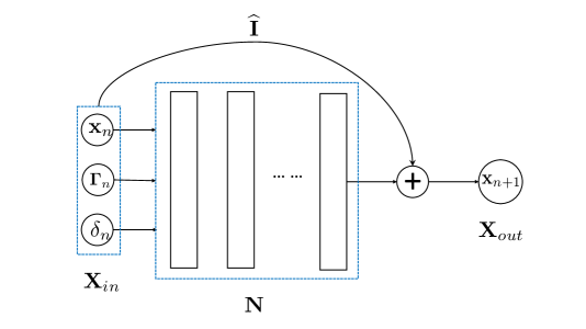
Inside the network, $\mathbf{N}:{\mathbb{R}}^{d+n_{b}+1}\to{\mathbb{R}}^{d}$ denotes the operator associated with a feed-forward neural network with $(d+n_{b}+1)$ input nodes and $d$ output nodes. The input is multiplied with $\widehat{\mathbf{I}}$ and then re-introduced back before the final output. The operator $\widehat{\mathbf{I}}\in{\mathbb{R}}^{d\times(d+n_{b}+1)}$ is a matrix of size ${d\times(d+n_{b}+1)}$. It takes the form

$$\widehat{\mathbf{I}}=[\mathbf{I}_{d},\mathbf{0}],$$ (20)

where $\mathbf{I}_{d}$ is identity matrix of size $d\times d$ and $\mathbf{0}$ is a zero matrix of size $d\times(n_{b}+1)$. Therefore, the network effectively defines a mapping

$$\mathbf{X}_{out}=\widehat{\mathbf{N}}(\mathbf{X}_{in};\Theta)=[\widehat{\mathbf{I}}+\mathbf{N}(\cdot;\Theta)](\mathbf{X}_{in}).$$ (21)

Training of the network is accomplished by using the training data set (18). For each of the $j$-th data entry, $j=1,\dots,J$, we set

$$\mathbf{X}_{in}^{(j)}\leftarrow[\mathbf{x}_{k}^{(j)};\bm{\Gamma}_{k}^{(j)};\delta_{k}^{(j)}]\in{\mathbb{R}}^{d+n_{b}+1}.$$ (22)

The network training is then conducted by minimizing the mean squared loss between the network output $\mathbf{X}_{out}^{(j)}$ and the data $\mathbf{x}_{k+1}^{(j)}$, i.e.,

$$\Theta^{*}=\operatornamewithlimits{argmin}_{\Theta}\frac{1}{J}\sum_{\j=1}^{J}\left\|\widehat{\mathbf{N}}(\mathbf{X}_{in}^{(j)};\Theta)-\mathbf{x}^{(j)}_{k+1}\right\|^{2}.$$ (23)

3.3.3 Learned Model and System Prediction

Upon satisfactory training of the network parameter using (23), we obtain a trained network model for the unknown modified system (14)

$$\mathbf{X}_{out}=\widehat{\mathbf{N}}(\mathbf{X}_{in};\Theta^{*})=[\widehat{\mathbf{I}}+\mathbf{N}(\cdot;\Theta^{*})](\mathbf{X}_{in}),$$ (24)

where $\widehat{\mathbf{I}}$ is defined in (20) and $\mathbf{N}$ is the operator of the FNN, as illustrated in the previous section and in Fig. 1.

For system prediction with a given external input function $\gamma(t)$, which is usually not in the training data set, let us consider the time instances (8). Let

$$\mathbf{X}_{in}=[\mathbf{x}(t_{n});\bm{\Gamma}_{n};\delta_{n}]$$

be a concatenated vector consisting of the state variable at $t_{n}$, the parameter vector for the local parameterization of the external input between $[t_{n},t_{n+1}]$, and $\delta_{n}=t_{n+1}-t_{n}$. Then, the trained model produces a one-step evolution of the solution

$$\widehat{\mathbf{x}}(t_{n+1})=\mathbf{x}(t_{n})+\mathbf{N}(\mathbf{x}(t_{n}),\bm{\Gamma}_{n},\delta_{n};\Theta^{*}).$$ (25)

Upon applying (25) recursively, we obtain a network model for predicting the system states of the unknown non-autonomous system (1). For a given initial condition $\mathbf{x}_{0}$ and external input $\gamma(t)$,

$$\left\{\begin{split}&\widehat{\mathbf{x}}(t_{0})=\mathbf{x}_{0},\\ &\widehat{\mathbf{x}}(t_{n+1})=\widehat{\mathbf{x}}(t_{n})+{\mathbf{N}}(\widehat{\mathbf{x}}(t_{n}),\bm{\Gamma}_{n},\delta_{n};\Theta^{*}),\\ &t_{n+1}=t_{n}+\delta_{n},\qquad n=0,\dots,N-1,\end{split}\right.$$ (26)

where $\bm{\Gamma}_{n}$ are the parameters in the local parameterization of $\gamma(t)$ in the time interval $[t_{n},t_{n+1}]$. It is obvious that the network predicting model (25) is an approximation to the one-step evolution (15) of the modified system (14), which in turn is an approximation of the original unknown dynamical system (1). Therefore, (26) generates an approximation to the solution of the unknown system (1) at the discrete time instances $\{t_{n}\}$ (8).

3.4 Theoretical Properties

We now present certain theoretical analysis for the proposed learning algorithm. The following result provides a bound between the solution of the modified system (14) and the original system (1). The difference between the two systems is due to the use of the parameterized external input $\widetilde{\gamma}(t)$ (12) in the modified system (14), as opposed to the original external input $\gamma(t)$ in the original system (1). Again, we emphasize that in many practical situations when the external input is already known in a parametric form, the modified system (14) is equivalent to the original system (1).

Proposition 2.

Consider the original system (1) with input $\gamma(t)$ and the modified system (14) with input $\widetilde{\gamma}(t)$ (12), and assume the function $\mathbf{f}(\mathbf{x},\gamma)$ is Lipschitz continuous with respect to both $\mathbf{x}$ and $\gamma$, with Lipschitz constants $L_{1}$ and $L_{2}$, respectively. If the difference in the inputs is bounded by

$$\|\gamma(t)-\widetilde{\gamma}(t)\|_{L^{\infty}([0,T])}\leq\eta,$$

where $T>0$ is a finite time horizon. Then,

$$|\mathbf{x}(t)-\widetilde{\mathbf{x}}(t)|\leq L_{2}\,\eta\,t\,e^{L_{1}t},\quad\forall t\in[0,T].$$

Proof.

For any $t\in[0,T]$,

$$\mathbf{x}(t) =\mathbf{x}(0)+\int_{0}^{t}\mathbf{f}(\mathbf{x}(s),\gamma(s))\,ds,$$

$$\widetilde{\mathbf{x}}(t) =\mathbf{x}(0)+\int_{0}^{t}\mathbf{f}(\widetilde{\mathbf{x}}(s),\widetilde{\gamma}(s))\,ds.$$

We then have

$$|\mathbf{x}(t)-\widetilde{\mathbf{x}}(t)| \leq\int^{t}_{0}|\mathbf{f}(\mathbf{x}(s),\gamma(s))-\mathbf{f}(\widetilde{\mathbf{x}}(s),\widetilde{\gamma}(s))|\,ds$$

$$\leq\int_{0}^{t}\lvert\mathbf{f}(\mathbf{x}(s),\gamma(s))-\mathbf{f}(\mathbf{x}(s),\widetilde{\gamma}(s))\rvert\,ds+\int_{0}^{t}\lvert\mathbf{f}(\mathbf{x}(s),\widetilde{\gamma}(s))-\mathbf{f}(\widetilde{\mathbf{x}}(s),\widetilde{\gamma}(s))\rvert\,ds$$

$$\leq L_{2}\int_{0}^{t}\lvert\gamma(s)-\widetilde{\gamma}(s)\rvert\,ds+L_{1}\int_{0}^{t}\lvert\mathbf{x}(s)-\widetilde{\mathbf{x}}(s)\rvert\,ds$$

$$\leq L_{2}\,\eta\,t+L_{1}\int_{0}^{t}\lvert\mathbf{x}(s)-\widetilde{\mathbf{x}}(s)\rvert\,ds.$$

By using Gronwall’s inequality, we obtain

$$|\mathbf{x}(t)-\widetilde{\mathbf{x}}(t)|\leq L_{2}\,\eta\,t\,e^{L_{1}t}.$$

∎

We now recall the celebrated universal approximation property of neural networks.

Proposition 3 ([16]).

For any function $F\in C(\mathbb{R}^{n})$ and a positive real number $\varepsilon>0$, there exists a single-hidden-layer neural network $N(\cdot\,;\Theta)$ with parameter $\Theta$ such that

$$\max_{\mathbf{y}\in D}|F(\mathbf{y})-N(\mathbf{y}\,;\Theta)|\leq\varepsilon,$$

for any compact set $D\in\mathbb{R}^{n}$, if and only if the activation functions are continuous and are not polynomials.

Relying on this result, we assume the trained neural network model (24) has sufficient accuracy, which is equivalent to assuming accuracy in the trained FNN operator $\mathbf{N}$ of (25) to the one-step evolution operator $\widetilde{\bm{\phi}}$ in (15). More specifically, let $\mathcal{D}$ be the convex hull of the training data set $\mathcal{S}$, defined (18). We then assume

$$\left\|\mathbf{N}(\cdot;\Theta^{*})-\widetilde{\bm{\phi}}(\cdot)\right\|_{L^{\infty}(\mathcal{D})}<\mathcal{E},$$ (27)

where $\mathcal{E}\geq 0$ is a sufficiently small real number.

Proposition 4.

Consider the modified system (15) and the trained network model (26) over the time instances (8). Assume the exact evolution operator (15) is Lipschitz continuous with respect to $\mathbf{x}$, with Lipschitz constant $L_{\phi}$. If the network training is sufficiently accurate such that (27) holds, then

$$\|\widehat{\mathbf{x}}(t_{n})-\widetilde{\mathbf{x}}(t_{n})\|\leq\frac{1-L_{\phi}^{n}}{1-L_{\phi}}\mathcal{E},\qquad n=0,\dots,N.$$ (28)

Proof.

Let $\bm{\Phi}=\widehat{\mathbf{I}}+\widetilde{\bm{\phi}}$, where $\widehat{\mathbf{I}}$ is defined in (20), we can rewrite the one-step evolution (15) as

$$\widetilde{\mathbf{x}}(t_{n+1})=[\bm{\Phi}(\cdot,\bm{\Gamma}_{n},\delta_{n})](\widetilde{\mathbf{x}}(t_{n})),$$

Meanwhile, the learned model (26) satisfies, by using (24),

$$\widehat{\mathbf{x}}(t_{n+1})=[\widehat{\mathbf{N}}(\cdot;\Theta^{*})](\widehat{\mathbf{x}}(t_{n})).$$

Let $e_{n}=\|\widehat{\mathbf{x}}(t_{n})-\widetilde{\mathbf{x}}(t_{n})\|$, we then have

$$\begin{split}e_{n}=&\left\|[\widehat{\mathbf{N}}(\cdot;\Theta^{*})](\widehat{\mathbf{x}}(t_{n-1}))-[\bm{\Phi}(\cdot,\bm{\Gamma}_{n-1},\delta_{n-1})](\widetilde{\mathbf{x}}(t_{n-1}))\right\|\\ \leq&\left\|[\widehat{\mathbf{N}}(\cdot;\Theta^{*})-\bm{\Phi}(\cdot,\bm{\Gamma}_{n-1},\delta_{n-1})](\widehat{\mathbf{x}}(t_{n-1}))\right\|+\\ &\left\|\left[\bm{\Phi}(\widehat{\mathbf{x}}(t_{n-1}),\bm{\Gamma}_{n-1},\delta_{n-1})\right]-\left[\bm{\Phi}(\widetilde{\mathbf{x}}(t_{n-1}),\bm{\Gamma}_{n-1},\delta_{n-1})\right]\right\|\\ \leq&~{}\mathcal{E}+L_{\phi}\left\|\widehat{\mathbf{x}}(t_{n-1})-\widetilde{\mathbf{x}}(t_{n-1})\right\|\end{split}$$

This gives

$$e_{n}\leq\mathcal{E}+L_{\phi}e_{n-1}.$$

Repeated use of this relation and with $e_{0}=0$ immediately gives the conclusion. ∎

Note that the assumption of Lipschitz continuity on the evolution operator in (15) is equivalent to assuming Lipschitz continuity on the right-hand-side of the original system (1). This is a very mild condition, commonly assumed for the well-posedness of the original problem (1).

Upon combining the results from above and using triangular inequality, we immediately obtain the following.

Theorem 5.

Under the assumptions of Proposition 2 and 4, the solution of the trained network model (26) and the true solution of the original system (1) over the time instances satisfies (8) satisfy

$$\left\|\widehat{\mathbf{x}}(t_{n})-\mathbf{x}(t_{n})\right\|\leq L_{2}\,\eta\,t_{n}\,e^{L_{1}t_{n}}+\frac{1-L_{\phi}^{n}}{1-L_{\phi}}\mathcal{E},\qquad n=0,\dots,N.$$ (29)

Remark 3.1.

It is worth noting that the DNN structure employed here is to accomplish the approximation (27). Such an approximation can be conducted by any other proper approximation techniques using, for example, (orthogonal) polynomials, Gaussian process, radial basis, etc. The target function is the one-step evolution operator $\widetilde{\bm{\phi}}$ in (15). Since for many problems of practical interest, $\widetilde{\bm{\phi}}:{\mathbb{R}}^{d+n_{b}+1}\to{\mathbb{R}}^{d}$ often resides in high dimensions and is highly nonlinear, DNN represents a more flexible and practical choice and is the focus of this paper.

4 Numerical Examples

In this section, we present numerical examples to verify the properties of the proposed methods. Since our purpose is to validate the proposed deep learning method, we employ synthetic data generated from known dynamical systems with known time-dependent inputs. The training data are generated by solving the known system with high resolution numerical scheme, e.g., 4th-order Runge Kutta with sufficiently small time steps. Our proposed learning method is then applied to the training data set. Once the learned model is constructed, we conduct system prediction using the model with new initial conditions and new external inputs. The prediction results are then compared with the reference solution obtained by solving the exact system with the same new inputs. Also, to clearly examine the numerical errors, we only present the tests where the training data do not contain noises.

In all the examples, we generate the training data set (2) with $K^{(i)}\equiv 2$, $\forall i$, i.e., each trajectory only contains two data points. For each of the $i$-th entry in the data set, the first data entry is randomly sampled from a domain $I_{\mathbf{x}}$ using uniform distribution. The second data entry is produced by solving the underlying reference dynamical system with a time step $\delta^{(i)}\in I_{\Delta}=[0.05,0.15]$ and subject to a parameterized external input in the form of (10), whose parameters (11) are uniformly sampled from a domain $I_{\bm{\Gamma}}$. The sampling domains $I_{\mathbf{x}}$ and $I_{\bm{\Gamma}}$ are problem specific and listed separately for each example.

The DNNs in all the examples use activation function $\sigma(x)=\tanh(x)$ and are trained by minimizing the mean squared loss function in (23). The network training is conducted by using Adam algorithm [9] with the open-source Tensorflow library [1]. Upon satisfactory training, the learned models are used to conduct system prediction, in the form of (26), with a constant step size $\delta_{n}=0.1$.

4.1 Linear Scalar Equation with Source

Let us first consider the following scalar equation

$$\frac{dx}{dt}=-\alpha(t)x+\beta(t),$$ (30)

where the time-dependent inputs $\alpha(t)$ and $\beta(t)$ are locally parameterized with polynomials of degree $2$, resulting the local parameter set (11) $\bm{\Gamma}_{n}\in{\mathbb{R}}^{n_{b}}$ with $n_{b}=3+3=6$. We build a neural network model consisting of $3$ hidden layers with $80$ nodes per layer. The model is trained with $20,000$ data trajectories randomly sampled, with uniform distribution, in the state variable domain $I_{\mathbf{x}}=[-2,2]$ and the local parameter domain $I_{\bm{\Gamma}}=[-5,5]^{6}$. After the network model is trained, we use it to conduct system prediction. In Fig. 2, the prediction result with a new initial condition $x_{0}=2$ and new external inputs $\alpha(t)=\sin(4t)+1$ and $\beta(t)=\cos(t^{2}/1000)$ is shown, for time up to $T=100$. The reference solution is also shown for comparison. It can be seen that the network model produces accurate prediction for this relatively long-term integration.

Fig. 2: DNN model prediction of (4.1) with external inputs $\alpha(t)=\sin(4t)+1$ and $\beta(t)=\cos(t^{2}/1000)$ and an initial condition $x_{0}=2$. Comparison of long-term neural network model prediction (labelled “NN”) with the reference solution.

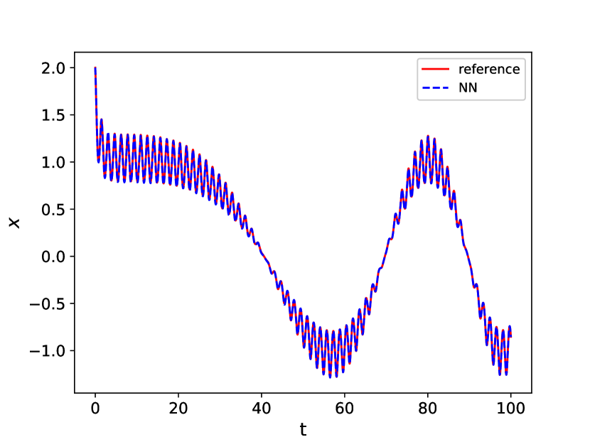
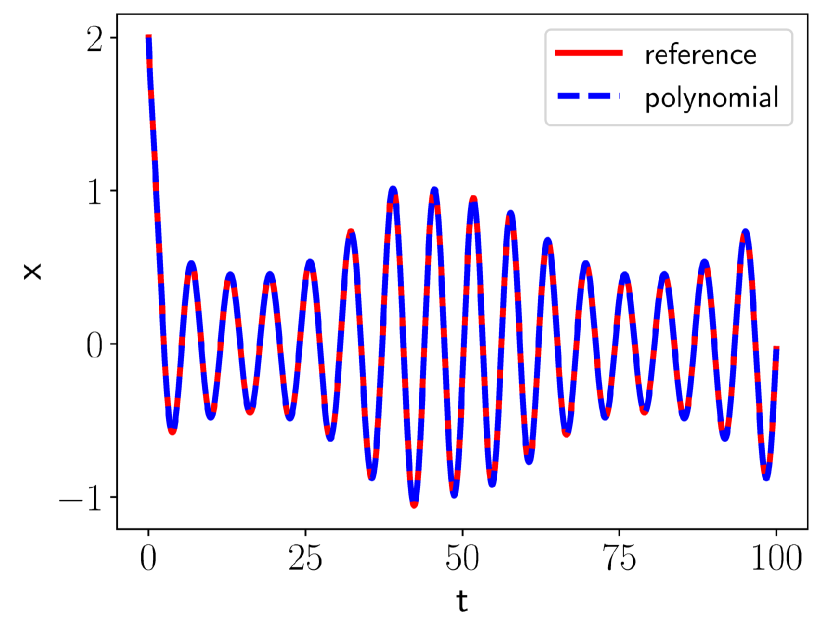
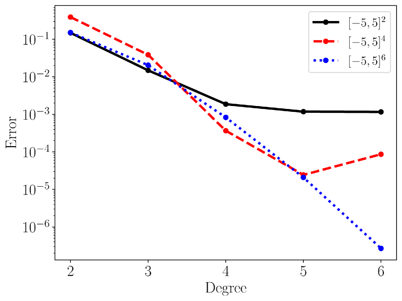
For this relatively simple and low-dimensional system, its learning can be effectively conducted by other standard approximation method, as discussed in Remark 3.1. With the same quadratic polynomial for local parameterization as in the DNN modeling, which results in $\bm{\Gamma}_{n}\in[-5,5]^{6}$, we employ tensor Legendre orthogonal polynomials in total degree space, which is a standard multi-dimensional approximation technique, for the approximation of the one-step evolution operator in (15). In Fig. 3, the prediction results by the polynomial learning model are shown, for a case with external inputs $\alpha(t)=\sin(t/10)+1$ and $\beta(t)=\cos(t)$. In Fig. 3(a), the prediction result obtained by 2nd-degree polynomial learning model is shown. We observe good agreement with the reference solution. In Fig. 3(b), the numerical errors at $T=100$ are shown for the polynomial learning model with varying degrees. We observe that the errors decay exponentially fast when the degree of polynomial is increased. Such kind of exponential error convergence is expected for approximation of smooth problems, such as this example.

(a) System prediction.

(b) Errors vs. polynomial degree.

Fig. 3: Polynomial learning model for (4.1) with $\alpha(t)=\sin(t/10)+1$ and $\beta(t)=\cos(t)$. (a) Comparison of the model prediction with reference solution. (b) Relative error in prediction at $T=100$ for increasing polynomial degree in the polynomial learning model. In all models piecewise quadratic polynomials are used for local parameterization.

4.2 Predator-prey Model with Control

We now consider the following Lotka-Volterra Predator-Prey model with a time-dependent input $u(t)$:

$$\begin{split}\dfrac{dx_{1}}{dt}&=x_{1}-x_{1}x_{2}+u(t),\\ \dfrac{dx_{2}}{dt}&=-x_{2}+x_{1}x_{2}.\end{split}$$ (31)

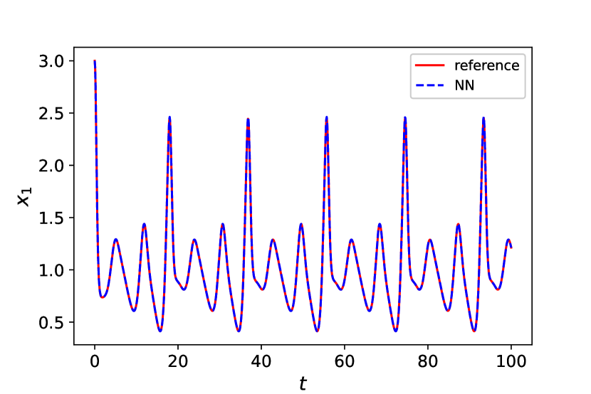
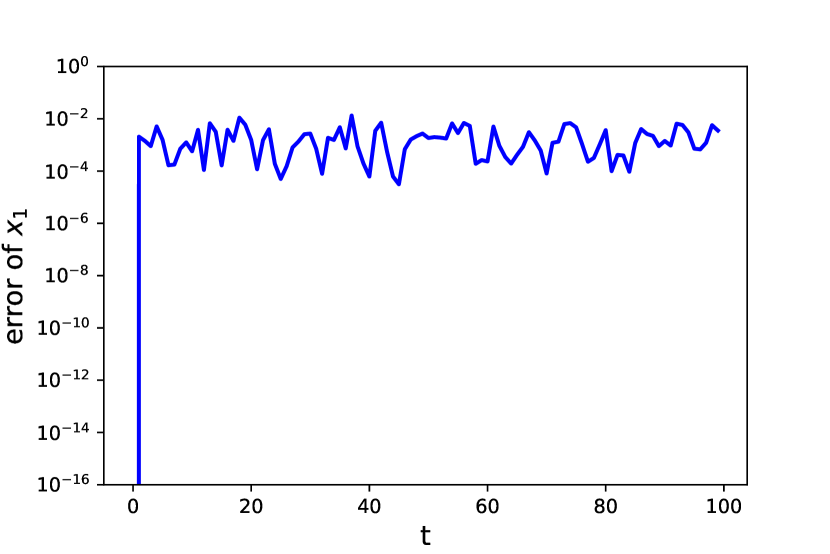
The local parameterization for the external input is conducted using quadratic polynomials, resulting in $\bm{\Gamma}_{n}\in{\mathbb{R}}^{3}$. More specifically, we set $I_{\bm{\Gamma}}=[0,5]^{3}$ and the state variable space $I_{\mathbf{x}}=[0,5]^{2}$. The DNN learning model consists of $3$ hidden layers, each of which with $80$ nodes. The network training is conducted using $20,000$ data trajectories randomly sampled from $I_{\mathbf{x}}\times I_{\bm{\Gamma}}$. In Fig. 4(a), we plot its prediction result for a case with $u(t)=\sin(t/3)+\cos(t)+2$, for time up to $T=100$, along with the reference solution. It can be seen that the DNN model prediction agrees very well with the reference solution. The numerical error fluctuates at the level of $O(10^{-3})$, for this relatively long-term prediction.

(a) System prediction of $x_{1}$.

(b) Error in prediction for $x_{1}$

Fig. 4: DNN learning model for (31). Comparison of its prediction result for $x_{1}$ with $u(t)=\sin(t/3)+\cos(t)+2$ against reference solution. Results for $x_{2}$ are very similar and not shown.

4.3 Forced Oscillator

We now consider a forced oscillator

$$\begin{split}\frac{dx_{1}}{dt}&=x_{2},\\ \frac{dx_{2}}{dt}&=-\nu(t)\,x_{1}-k\,x_{2}+f(t),\end{split}$$ (32)

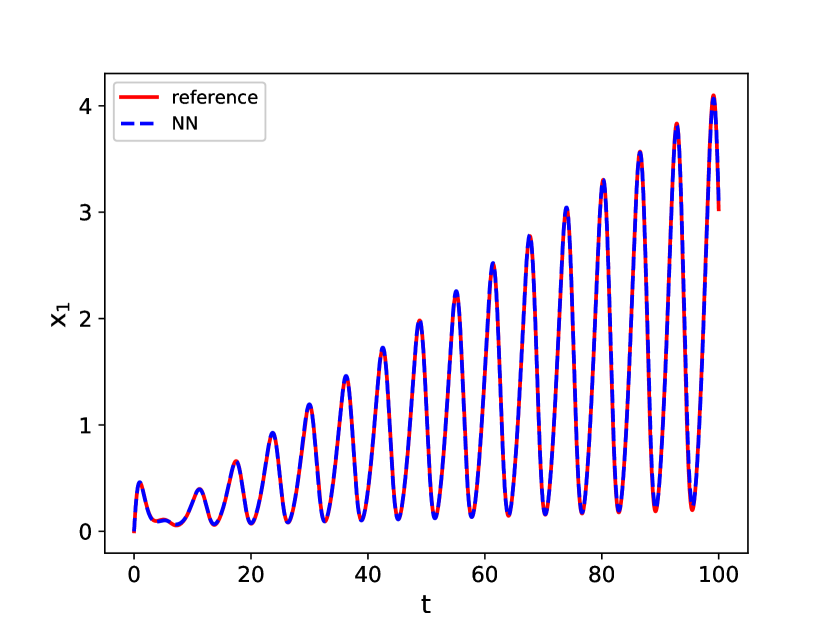
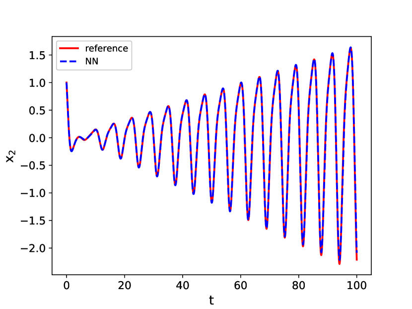
where the damping term $\nu(t)$ and the forcing $f(t)$ are time-dependent processes. Local parameterization for the inputs is conducted using quadratic polynomials. More specifically, the training data are generated randomly by sampling from state variable space $I_{\mathbf{x}}=[-3,3]^{2}$ and local parameterization space $I_{\bm{\Gamma}}=[-3,3]^{6}$. Similar to other examples, the DNN contains $3$ hidden layers with $80$ nodes in each hidden layer. System prediction using the trained network model is shown in Fig. 5, for rather arbitrarily chosen external inputs $\nu(t)=\cos(t)$ and $f(t)=t/50$. Once again, we observe very good agreement with the reference solution for relatively long-term simulation up to $T=100$.

(a) $x_{1}(t)$

(b) $x_{2}(t)$

Fig. 5: DNN model prediction of (32) with inputs $\nu(t)=\cos(t)$ and $f(t)=t/50$.

4.4 PDE: Heat Equation with Source

We now consider a partial differential equation (PDE). In particular, the following heat equation with a source term,

$$\begin{split}&u_{t}=u_{xx}+q(t,x),\quad x\in[0,1],\\ &u(0,x)=u_{0}(x),\\ &u(t,0)=u(t,1)=0,\end{split}$$ (33)

where $q(t,x)$ is the source term varying in both space and time. We set the source term to be

$$q(t,x)=\alpha(t)e^{-\frac{(x-\mu)^{2}}{\sigma^{2}}},$$

where $\alpha(t)$ is its time varying amplitude and parameter $\mu$ and $\sigma$ determine its the spatial profile.

The learning of (33) is conducted in a discrete space. Specifically, we employ $n=22$ equally distributed grid points in the domain $[0,1]$,

$$x_{j}=j/(n-1),\qquad j=1,\dots,n.$$

Let

$$\mathbf{u}(t)=\left[u(t,x_{2}),\cdots,u(t,x_{n-1})\right]^{\dagger},$$

we then seek to construct a DNN model to discover the dynamical behavior of the solution vector $\mathbf{u}(t)$. Note that the boundary values $u(x_{1})=u(x_{n})=0$ are fixed in the problem setting and to be included in the learning model.

Upon transferring the learning of the PDE (33) into learning of a finite dimensional dynamical system of $\mathbf{u}\in{\mathbb{R}}^{d}$, where $d=n-2=20$, the DNN learning method discussed in this paper can be readily applied. Training data are synthetic data generated by solving the system (33) numerically. In particular, we employ second-order central difference scheme using the same grid points $\{x_{j}\}$. The trajectory data are generated by randomly sample $\mathbf{u}\in{\mathbb{R}}^{20}$ in a specific domain $I_{\mathbf{u}}=[0,2]^{20}$. Quadratic polynomial interpolation is used in local parameterization of the time dependent source term, resulting in 3-dimensional local representation for the time dependent coefficient $\alpha(t)$. Random sampling in domain $I_{\alpha}=[-2,2]^{3}$, $I_{\mu}=[0,3]$, $I_{\sigma}=[0.05,0.5]$ is then used to generate the synthetic training data set, for the parameters $\alpha$, $\mu$, and $\sigma$, respectively.

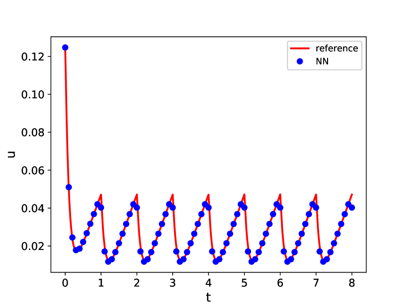
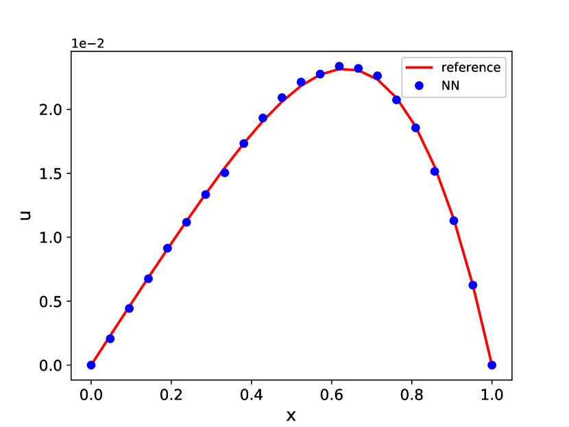
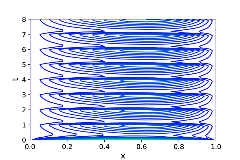
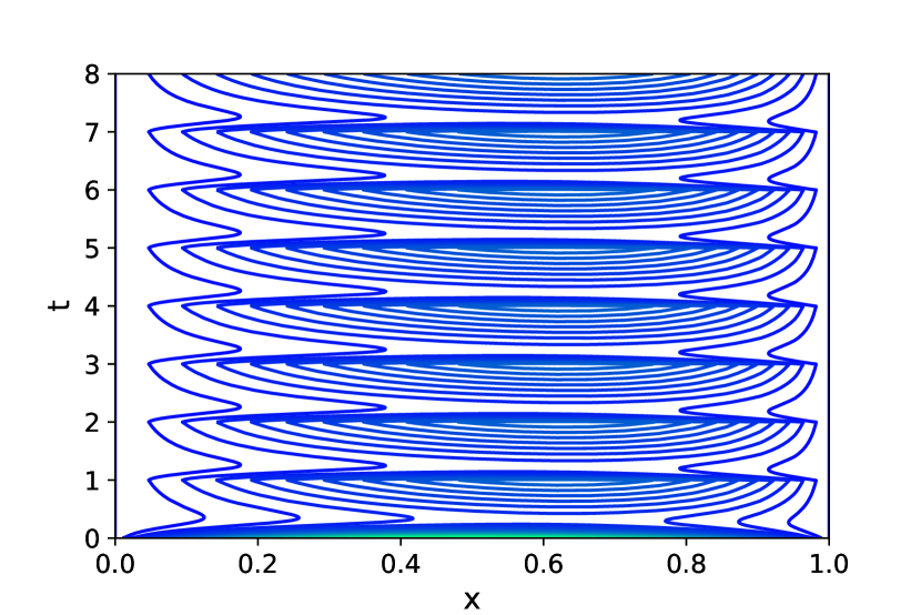
The DNN network model thus consists of a total of $25$ inputs. Because of curse-of-dimensionality, constructing accurate approximation in 25 dimensional space is computational expensive via traditional methods such as polynomials, radial basis, etc. For DNN, however, 25 dimension is considered low and accurate network model can be readily trained. Here we employ a DNN with $3$ hidden layers, each of which with $80$ nodes. Upon successful training of the DNN model, we conduct system prediction for a new source term (not in training data set), where $\alpha(t)=t-\lfloor t\rfloor$ is a saw-tooth discontinuous function, $\mu=1$, and $\sigma=0.5$.

The system prediction results are shown in Fig. 6, along with the reference solution solved from the underlying PDE. We observe excellent agreement between the DNN model prediction to the reference solution. It is worth noting that the DNN model, once trained, can be readily used to predict system behavior for other time dependent inputs.

(a) Solution evolution at $x=0.5$

(b) Solution profile at $t=2$

(c) Reference solution contours over time

(d) DNN prediction contours over time

Fig. 6: System prediction of (33) with $\alpha(t)=t-\lfloor t\rfloor$, $\mu=1$, and $\sigma=0.5$. Comparison between the predictions by the DNN model and the reference solution.

5 Conclusion

In this paper we presented a numerical approach for learning unknown non-autonomous dynamical systems using observations of system states. To circumvent the difficulty posed by the non-autonomous nature of the system, the system states are expressed as piecewise integrations over time. The piecewise integrals are then transformed into parametric form, upon a local parameterization procedure of the external time-dependent inputs. We then designed deep neural network (DNN) structure to model the parametric piecewise integrals. Upon using sufficient training data to train the DNN model, it can be used recursively over time to conduct system prediction for other external inputs. Various numerical examples in the paper suggest the methodology holds promise to more complex applications.

References

- [1] M. Abadi, A. Agarwal, P. Barham, E. Brevdo, Z. Chen, C. Citro, G. S. Corrado, A. Davis, J. Dean, M. Devin, S. Ghemawat, I. Goodfellow, A. Harp, G. Irving, M. Isard, Y. Jia, R. Jozefowicz, L. Kaiser, M. Kudlur, J. Levenberg, D. Mané, R. Monga, S. Moore, D. Murray, C. Olah, M. Schuster, J. Shlens, B. Steiner, I. Sutskever, K. Talwar, P. Tucker, V. Vanhoucke, V. Vasudevan, F. Viégas, O. Vinyals, P. Warden, M. Wattenberg, M. Wicke, Y. Yu, and X. Zheng, TensorFlow: Large-scale machine learning on heterogeneous systems, 2015, https://www.tensorflow.org/. Software available from tensorflow.org.
- [2] S. L. Brunton, J. L. Proctor, and J. N. Kutz, Discovering governing equations from data by sparse identification of nonlinear dynamical systems, Proc. Natl. Acad. Sci. U.S.A., 113 (2016), pp. 3932–3937.
- [3] S. L. Brunton, J. L. Proctor, and J. N. Kutz, Sparse identification of nonlinear dynamics with control (sindyc), IFAC-PapersOnLine, 49 (2016), pp. 710–715.
- [4] Z. Chen and D. Xiu, On generalized residue network for deep learning of unknown dynamical systems, arXiv preprint arXiv:2002.02528, (2020).
- [5] X. Fu, L.-B. Chang, and D. Xiu, Learning reduced systems via deep neural networks with memory, J. Machine Learning Model. Comput., 1 (2020).
- [6] N. Galioto and A. A. Gorodetsky, Bayesian system id: optimal management of parameter, model, and measurement uncertainty, (2020), https://arxiv.org/abs/2003.02359. Submitted.
- [7] K. He, X. Zhang, S. Ren, and J. Sun, Deep residual learning for image recognition, in Proceedings of the IEEE conference on computer vision and pattern recognition, 2016, pp. 770–778.
- [8] I. G. Kevrekidis, C. W. Gear, J. M. Hyman, P. G. Kevrekidid, O. Runborg, C. Theodoropoulos, et al., Equation-free, coarse-grained multiscale computation: Enabling mocroscopic simulators to perform system-level analysis, Commun. Math. Sci., 1 (2003), pp. 715–762.
- [9] D. P. Kingma and J. Ba, Adam: A method for stochastic optimization, arXiv preprint arXiv:1412.6980, (2014).
- [10] Z. Long, Y. Lu, and B. Dong, Pde-net 2.0: Learning pdes from data with a numeric-symbolic hybrid deep network, Journal of Computational Physics, 399 (2019), p. 108925.
- [11] Z. Long, Y. Lu, X. Ma, and B. Dong, PDE-net: learning PDEs from data, in Proceedings of the 35th International Conference on Machine Learning, J. Dy and A. Krause, eds., vol. 80 of Proceedings of Machine Learning Research, Stockholmsmässan, Stockholm Sweden, 10–15 Jul 2018, PMLR, pp. 3208–3216.
- [12] N. M. Mangan, J. N. Kutz, S. L. Brunton, and J. L. Proctor, Model selection for dynamical systems via sparse regression and information criteria, Proceedings of the Royal Society of London A: Mathematical, Physical and Engineering Sciences, 473 (2017).
- [13] I. Mezić, Spectral properties of dynamical systems, model reduction and decompositions, Nonlinear Dynamics, 41 (2005), pp. 309–325.
- [14] I. Mezić, Analysis of fluid flows via spectral properties of the koopman operator, Annual Review of Fluid Mechanics, 45 (2013), pp. 357–378.
- [15] B. Peherstorfer and K. Willcox, Data-driven operator inference for nonintrusive projection-based model reduction, Computer Methods in Applied Mechanics and Engineering, 306 (2016), pp. 196–215.
- [16] A. Pinkus, Approximation theory of the MLP model in neural networks, Acta Numerica, 8 (1999), pp. 143–195.
- [17] J. L. Proctor, S. L. Brunton, and J. N. Kutz, Dynamic mode decomposition with control, SIAM Journal on Applied Dynamical Systems, 15 (2016), pp. 142–161.
- [18] J. L. Proctor, S. L. Brunton, and J. N. Kutz, Generalizing koopman theory to allow for inputs and control, SIAM Journal on Applied Dynamical Systems, 17 (2018), pp. 909–930.
- [19] T. Qin, Z. Chen, J. Jakeman, and D. Xiu, A neural network approach for uncertainty quantification for time-dependent problems with random parameters, arXiv preprint arXiv:1910.07096, (2019).
- [20] T. Qin, K. Wu, and D. Xiu, Data driven governing equations approximation using deep neural networks, Journal of Computational Physics, 395 (2019), pp. 620–635.
- [21] M. Raissi, Deep hidden physics models: Deep learning of nonlinear partial differential equations, The Journal of Machine Learning Research, 19 (2018), pp. 932–955.
- [22] M. Raissi, P. Perdikaris, and G. E. Karniadakis, Machine learning of linear differential equations using gaussian processes, Journal of Computational Physics, 348 (2017), pp. 683–693.
- [23] M. Raissi, P. Perdikaris, and G. E. Karniadakis, Multistep neural networks for data-driven discovery of nonlinear dynamical systems, arXiv preprint arXiv:1801.01236, (2018).
- [24] R. Rico-Martinez and I. G. Kevrekidis, Continuous time modeling of nonlinear systems: A neural network-based approach, in IEEE International Conference on Neural Networks, IEEE, 1993, pp. 1522–1525.
- [25] S. H. Rudy, J. N. Kutz, and S. L. Brunton, Deep learning of dynamics and signal-noise decomposition with time-stepping constraints, Journal of Computational Physics, 396 (2019), pp. 483–506.
- [26] P. J. Schmid, Dynamic mode decomposition of numerical and experimental data, Journal of fluid mechanics, 656 (2010), pp. 5–28.
- [27] C. Theodoropoulos, Y.-H. Qian, and I. G. Kevrekidis, “coarse” stability and bifurcation analysis using time-steppers: A reaction-diffusion example, Proceedings of the National Academy of Sciences, 97 (2000), pp. 9840–9843.
- [28] K. Wu, T. Qin, and D. Xiu, Structure-preserving method for reconstructing unknown hamiltonian systems from trajectory data, arXiv preprint arXiv:1905.10396, (2019).
- [29] K. Wu and D. Xiu, Numerical aspects for approximating governing equations using data, Journal of Computational Physics, 384 (2019), pp. 200–221.
- [30] K. Wu and D. Xiu, Data-driven deep learning of partial differential equations in modal space, Journal of Computational Physics, 408 (2020), p. 109307.