RODE-Net: Learning Ordinary Differential Equations with Randomness from Data

Abstract

Random ordinary differential equations (RODEs), i.e. ODEs with random parameters, are often used to model complex dynamics. Most existing methods to identify unknown governing RODEs from observed data often rely on strong prior knowledge. Extracting the governing equations from data with less prior knowledge remains a great challenge. In this paper, we propose a deep neural network, called RODE-Net, to tackle such challenge by fitting a symbolic expression of the differential equation and the distribution of parameters simultaneously. To train the RODE-Net, we first estimate the parameters of the unknown RODE using the symbolic networkslong2019pde by solving a set of deterministic inverse problems based on the measured data, and use a generative adversarial network (GAN) to estimate the true distribution of the RODE’s parameters. Then, we use the trained GAN as a regularization to further improve the estimation of the ODE’s parameters. The two steps are operated alternatively. Numerical results show that the proposed RODE-Net can well estimate the distribution of model parameters using simulated data and can make reliable predictions. It is worth noting that, GAN serves as a data driven regularization in RODE-Net and is more effective than the $\ell_{1}$ based regularization that is often used in system identifications.

1 Introduction

In the study of complex systems such as fluid dynamics, soft materials, biological evolution, etc., we often introduce empirical formulas and parameters into differential equations to model complex macroscopic phenomena induced by microscopic behaviors. These include for example, the sub-grid stress in turbulence models, high order moment closure for moment equations, the drag coefficient which expressed as a function of porosity in particle fluid problem, and a variety of empirical formulas in biological and economical models. However, drawbacks of using empirical formulas and parameters to model such complex systems are that: 1) for systems with non-separable scales, it is difficult to directly deduce accurate macroscopic equations based on microscopic mechanism; 2) models with fixed parameters cannot reflect the inherent randomness of the system, and hence can only crudely approximate the system in the average sense. Therefore, to address the above issues, we propose a machine learning framework to learn both the expression of differential equations and the distribution of the associated random parameters simultaneously.

1.1 Related Work

We start with a review of inverse problems for deterministic systems. Under the premise that the explicit form of the differential equation is known, the optimal parameters can be learned from the observed data by using classical system identification and tools from inverse problems. Several works lin2008learning ; liu2010learning ; long2018pde ; patel2018nonlinear solved a class of inverse problems under weaker assumptions based on the idea of unrolling dynamics of the numerical integration in the time direction. In raissi2018hidden , the authors proposed to use neural network as a surrogate to learn optimal parameters. When the explicit formula of the equation is unknown, brunton2016discovering constructed a dictionary consisted of simple terms that are likely to appear in the equations and employ sparse regression methods to select candidates for the expression of the equations. A series of works bongard2007automated ; schmidt2009distilling ; xu2020dlga used genetic algorithms to discover the underlying terms of the differential equations. In long2019pde , the authors proposed a deep symbolic neural network, called SymNet, to estimate the unknown expression of the differential equations, which has a relatively low memory requirement and computational complexity in many cases.

For problems with randomness, uncertainty quantification methods smith2013uncertainty are often adopted to study forward uncertainty propagation (e.g., liu1986probabilistic ; zhang2001stochastic ; ghanem2003stochastic ; xiu2010numerical ). However, it is generally much more difficult to study inverse problems with uncertainty than forward uncertainty propagation. In earlier work, kennedy2001bayesian proposed a 4-steps modular Bayesian approach to calibrate parameters of models. In chen2019learning , neural networks were used to estimate the modes of K-L expansion during the study of the forward and inverse problems of stochastic advection-diffusion-reaction equations. Based on PINN raissi2018hidden , yang2020b estimated the posterior of model parameters by Hamiltonian Monte Carlo and variational inference. The most related work to ours is yang2018physics , where the authors introduced a generative adversarial network (GAN) goodfellow2014generative ; arjovsky2017wasserstein ; gulrajani2017improved to estimate the distribution of data snapshots. These works further advanced the development of inverse uncertainty quantification. However, Bayesian based framework kennedy2001bayesian ; chen2019learning ; yang2020b often suffers from the curse of dimensionality. Although the use of GAN by yang2018physics can overcome the curse of dimensionality, it also requires a relatively strong prior knowledge on the differential equation to be identified. Furthermore, the GAN of yang2018physics were not specifically designed to estimate the distribution of the parameters of the differential equations.

In this paper, we propose a new machine learning framework for inverse uncertainty quantification. We introduce a new model, called RODE-Net, to estimate random ordinary differential equations (RODEs) from observed data by combining SymNet long2019pde for system identification and GAN goodfellow2014generative ; arjovsky2017wasserstein ; gulrajani2017improved for parameters distribution estimation. The high expressive power of SymNet enables the proposed RODE-Net to assume only minor prior knowledge on the form of the RODE to be identified. A particular novelty of the propose model is that, unlike existing inverse uncertainty quantification methods, RODE-Net estimates the distribution of parameters and makes use of GAN as a data driven regularization.

We note that, using GAN as a data driven regularization is common in image restoration bora2017compressed ; shah2018solving ; ledig2017photo . For example, bora2017compressed ; shah2018solving put forward the idea that we could solve image restoration problems within the range of a well trained GAN. In ledig2017photo the authors used discriminator as the regularization in image super resolution problems. These latest studies in computer vision inspired us to use GAN as a data driven regularization which is new to inverse uncertainty quantification.

The rest of the paper is organized as follows. In Section 2, we introduce the architecture of RODE-Net. Details on training and the loss functions are introduced in Section 3. Experiments are presented in Section 4, and we conclude the paper in Section 5.

2 The RODE-Net

Given a set of observed time series $\{\bm{x}(t)\}\subset\mathbb{R}^{d}$ with $d$ being the dimension of the observable quantities, we aim to discover the governing RODE from the set of time series. We assume that the RODE to be discovered takes the following form:

$$\frac{d\bm{x}}{dt}=\bm{F}_{\bm{\eta}}(\bm{x}),\bm{x}=(x_{1},\cdots,x_{d})\in\mathbb{R}^{d},t\geq 0$$ (1)

where $\bm{F}_{\bm{\eta}}(\cdot):\mathbb{R}^{d}\to\mathbb{R}^{d}$ is a $d$ dimensional vector function and $\bm{\eta}\sim\mathcal{P}$ is the random parameter of $\bm{F}_{\bm{\eta}}$. The RODE describes an infinite set of ODEs determined by the distribution of the random vector $\bm{\eta}$. For each random realization of the random variable ${\bm{\eta}}$, denoted as ${\bm{\eta}}_{i}$, we call the associated ODE as ODE-${\bm{\eta}}_{i}$. We note that the RODEs in this paper are different from those considered in han2017random ; neckel2013random . To obtain solutions with higher regularities, the latter considers system parameters as random processes (e.g. solution of SDEs) rather than random variables.

Consider the data set $X:=\{\bm{x}_{\bm{\eta}_{i}}^{j}(t_{k}):1\leq i\leq M,1\leq j\leq N_{i},0\leq k\leq S\}$, where $M$ is the number of realizations of ODE-${\bm{{\bm{\eta}}}}$. In practice, the data set $X$ is measured from the real world. As a proof of concept and to validate the proposed RODE-Net, in our experiments in Section 4, we generate data $\bm{x}_{\bm{\eta}_{i}}^{j}(t_{k})$ by solving ODE-${\bm{\eta}}_{i}$ using the fourth order Runge-Kutta method with $N_{i}$ different initial values $\bm{x}_{\bm{\eta}_{i}}^{j}(t_{0}),j=1,\cdots,N$.

Our proposed RODE-Net (Fig. 1) is designed to identify each individual ODE of {ODE-${\bm{\eta}}_{i}$ $:1\leq i\leq M$} and to estimate the distribution of ${\bm{\eta}}$ from $\{\bm{\eta}_{i}:1\leq i\leq M\}$ at the same time. To achieve both objectives, the RODE-Net framework consists of two main components:

1. A set of SymNet-based ODE-Nets which aim to estimate $\bm{F}_{\bm{\eta}_{i}}$ of each individual ODE;

2. A GAN to learn the distribution of $\{{\bm{\eta}}_{i}\}$.

The trained GAN represents the distribution $\mathcal{P}$ of the RODE and is able to generate ODE instances ODE-${\bm{\eta}}$. Moreover, we note that the GAN also serves as a good regularization in the training of ODE-Nets.

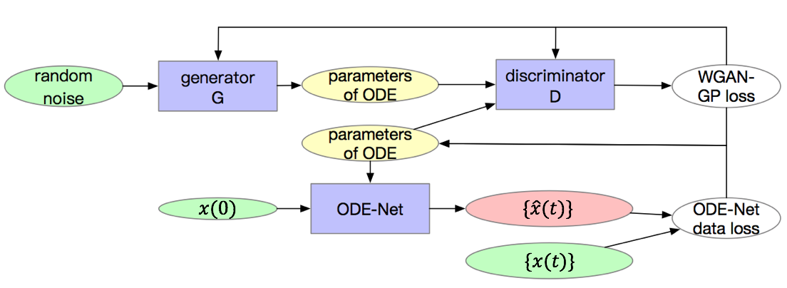
Figure 1: The pipeline of RODE-Net. The modules in green indicate input data; the modules in yellow indicate intermediate outputs; the module in red indicates the final output; the modules in blue indicate those with trainable parameters; and the modules in white indicate the loss functions.

2.1 The ODE-Net Component

For each ODE-${\bm{\eta}}_{i}$, the associated ODE-Net is a reduced version of PDE-Net 2.0 long2019pde , which can be constructed through unrolled forward Euler numerical discretization. One $\delta t$-block of the $l$-th component of the ODE-Net estimating ODE-${\bm{\eta}_{i}}$ can be written as:

$$\hat{x}_{l}(t+\delta t)=\hat{x}_{l}(t)+\delta t\cdot\text{SymNet}^{\alpha}_{d}(\hat{\bm{x}}(t);\hat{{\bm{\xi}}}_{i}^{(l)}),\hat{\bm{x}}(t)=(\hat{x}_{1}(t),\cdots,\hat{x}_{d}(t)),l=1,\cdots,d,$$ (2)

where $\bm{\hat{x}}(0)=\bm{x}(0)$ which is the initial value of ODE-${\bm{\eta}_{i}}$ and $\text{SymNet}^{\alpha}_{d}$ is a network that takes a $d$ dimensional vector as input and has $\alpha$ hidden layers, which can approximate polynomials of input variables and is able to output the expression of the equation through symbolic computations $s(\cdot)$. In practice, we take $\alpha=2$. Here, $\hat{{\bm{\xi}}}_{i}=(\hat{{\bm{\xi}}}_{i}^{(1)},\cdots,\hat{{\bm{\xi}}}_{i}^{(d)})$ are the trainable parameters of ODE-Net, and $s(\hat{{\bm{\xi}}}_{i})$ is an estimation of ${\bm{\eta}}_{i}$. Fig. 2 (a) shows the architecture of the ODE-Net.

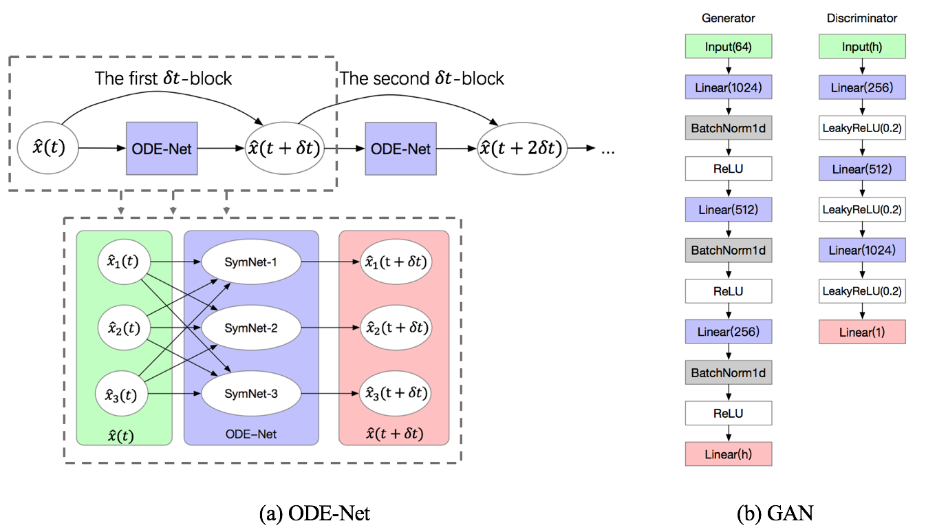
Figure 2: The architecture of the ODE-Net and the GAN

2.2 The GAN Component

It is natural to apply GAN to $\{s(\hat{\bm{\xi}_{i}})\}_{i}$ to estimate the distribution of $\bm{\eta}$. However, it is difficult (and unnecessary) to take derivative on the symbolic computation $s$. Therefore, in RODE-Net, we choose to use GAN to approximate the distribution of $\{\hat{\bm{\xi}_{i}}\}_{i}$ instead. By doing so, we can still provide a viable approximation of the distribution of $\bm{\eta}$ by simply taking the symbolic computations after the estimation of the distribution of $\{\hat{\bm{\xi}_{i}}\}_{i}$.

In RODE-Net, we adopt WGAN (Wasserstein GAN) goodfellow2014generative ; arjovsky2017wasserstein to draw the distribution of ${\bm{\xi}}$ by solving the following constrained minimax problem:

$$\min_{G}\max_{D}\mathbb{E}_{{\bm{\xi}}\sim\mathcal{P}_{\bm{\xi}}}D({\bm{\xi}})-\mathbb{E}_{\tilde{{\bm{\xi}}}\sim\mathcal{P}_{g}}D(\tilde{{\bm{\xi}}})\quad s.t.||D||_{L}\leq 1.$$ (3)

where $D$ is a discriminator and $\mathcal{P}_{g}$ is the distribution implicitly defined by the generator $G$: $\tilde{{\bm{\xi}}}=G(z),z\sim p_{z}$. Since the true data ${\bm{\xi}}$ are not directly observable, the training samples ${\bm{\xi}}\sim\mathcal{P}_{\bm{\xi}}$ are approximately generated by $\hat{{\bm{\xi}}}\sim\mathcal{P}_{\hat{{\bm{\xi}}}}$, i.e. the parameters of ODE-Nets which can be learned from the observed data (Sec2.1). In RODE-Net, $G$ and $D$ are neural networks with multiple fully connected hidden layers and non-linear activation functions. The architecture of the generator and discriminator is shown in Fig. 2 (b). The dimension of both the output of the generator and the input of the discriminator are equal to the size of each $\hat{\bm{\xi}_{i}}$, which is $d\cdot(\alpha^{2}+2d\cdot\alpha+d+2\alpha+1)$.

3 Training

The training of RODE-Net has three stages which include two warm-up stages and the alternating stage. In the first stage (warm-up-1), we train the ODE-Nets from the observed data. Secondly (warm-up-2), we train the GAN using the estimated parameters of the ODE-Nets. Thirdly (alternating stage), the GAN is used as a regularization to further improve the estimates on the parameters of the ODE-Nets by updating the parameters of GAN and ODE-Nets alternatively.

Warm-up-1:

Given each $X_{i}:=\{\bm{x}_{\bm{\eta}_{i}}^{j}(t_{k}):1\leq j\leq N_{i},0\leq k\leq S\}$ with $1\leq i\leq M$, the parameters of the associated ODE-Net can be learned by solving the following minimization problem:

$$\min_{\hat{\bm{\xi}}_{i}}\frac{1}{N_{i}}\sum_{j=1}^{N_{i}}L_{\text{data}}(\hat{\bm{\xi}}_{i},\bm{x}_{\bm{\eta}_{i}}^{j}(t))+\lambda_{h}L_{\text{Huber}}(\hat{\bm{\xi}}_{i}).$$ (4)

Here, the data loss term $L_{\text{data}}(\hat{\bm{\xi}}_{i},\bm{x}_{\bm{\eta}_{i}}^{j}(t))=\sum_{k=1}^{\tilde{S}}w_{k}\|\hat{\bm{x}}_{\bm{\eta}_{i}}^{j}(t_{k})-\bm{x}_{\bm{\eta}_{i}}^{j}(t_{k})||_{2}^{2}/\delta t^{2},\quad\tilde{S}\leq S,$ describes the accuracy of the ODE-Net to match the data $X_{i}$, where $w_{k}=\frac{e^{k}}{\sum_{s=1}^{\tilde{S}}e^{s}}$. The regularization term $L_{\text{Huber}}$ is defined as follows:

$$L_{\text{Huber}}(\hat{\bm{\xi}}_{i})=\sum_{p\text{ is a component of }\hat{\bm{\xi}}_{i}}\ell_{s}(p),\quad\mbox{and}\quad\ell_{s}(p)=\begin{cases}|p|-\frac{s}{2}&\text{if \,}|p|>s\\ \frac{1}{2s}p^{2}&\text{else}\end{cases}.$$ (5)

This is known as the Huber function which is a smoothed version of the absolute value. The hyperparameters $\lambda_{h}=s=0.001$ are used in RODE-Net.

During the training of the ODE-Nets, we adopt a strategy to gradually increase the number of steps $\tilde{S}$ from 1 to $S_{\text{max}}$. This strategy is to ensure the accuracy of long-term prediction and to keep the model stable during training. In practice we take $S_{\text{max}}=6$. We use Adam kingma2014adam to minimize the above loss function with a learning rate of 0.01.

Warm-up-2:

The learned parameters $\{\hat{\bm{\xi}}_{i}=(\hat{\bm{\xi}}_{i}^{(1)},\cdots,\hat{\bm{\xi}}_{i}^{(d)})\}$ in Warm-up-1 serve as training data for WGAN. To improve training of WGAN, we adopt the gradient penalty methods gulrajani2017improved , i.e. solving the following WGAN-GP problem which is a penalized version of the original WGAN problem:

$$\min_{G}\max_{D}\mathbb{E}_{{\bm{\xi}}\sim\mathcal{P}_{\bm{\xi}}}D({\bm{\xi}})-\mathbb{E}_{z\sim p_{z}}D(G(z))-\lambda_{gp}\mathbb{E}_{{\bm{\xi}}^{\prime}\sim\mathcal{P}_{{\bm{\xi}}^{\prime}}}(\|\nabla_{{\bm{\xi}}^{\prime}}D({\bm{\xi}}^{\prime})\|_{2}-1)^{2},$$ (6)

where we define $\mathcal{P}_{{\bm{\xi}}^{\prime}}$ by sampling uniformly along straight lines between ${\bm{\xi}}\sim\mathcal{P}_{\bm{\xi}}$ and $G(z)$ with $z\sim p_{z}$. Moreover, $\mathcal{P}_{\bm{\xi}}$ is approximated by $\mathcal{P}_{\hat{{\bm{\xi}}}}$. We update $G$ and $D$ alternatively by optimizing the WGAN-GP loss (6) where we take $\lambda_{gp}=10$.

Alternating stage:

In the warm-up-1 stage, each of the ODE-Net is estimated only using the data $X_{i}$. This has two potential problems: 1) some instances of the underlying RODE may be harder to estimate than others; 2) the estimate of each ODE does not make use of the fact that it is an instance from a RODE. Therefore, to provide an estimate of the ODE instances with a uniform control of quality and to take advantage of the entire data set $X$, we use GAN as a regularization and update the parameters of GAN and the ODE-Nets alternatively.

In addition to the data and the Huber loss term introduced in (4), we introduce another loss term, GAN regularization: $L_{\text{GANreg}}(\hat{\bm{\xi}})=D(\hat{\bm{\xi}}).$ The regularization by GAN can be interpreted as a switching of the role of the generator and the ODE-Nets, which enforces the parameters of the ODE-Nets to be similar to what can be generated by the learned generator. The full loss used in this stage is

$$L_{\text{rodenet}}(\hat{\bm{\xi}}_{i};\bm{x}_{\bm{\eta}_{i}}(t))=\frac{1}{N_{i}}\sum_{j}L_{\text{data}}(\hat{\bm{\xi}_{i}},\bm{x}_{\bm{\eta}_{i}}^{j}(t))+\lambda_{h}L_{\text{Huber}}(\hat{\bm{\xi}}_{i})+\lambda_{G}L_{\text{GANreg}}(\hat{\bm{\xi}}_{i}),$$ (7)

where we take $\lambda_{G}=0.1$ in practice.

The alternating update of the ODE-Nets and GAN is a mixed procedure of warm-up-1 and warm-up-2, except that we have modified the loss of training ODE-Nets. The training of the RODE-Net consists of this algorithm, together with warm-up-1 and warm-up-2, and is detailed in Algorithm 1.

Algorithm 1 RODE-Net Training: rode-net-train($\theta,V,\bm{\xi},\bm{x}(t))$.
The hyperparameters are set to $n_{d}=1,n_{\text{GAN}}=100$. The parameters of ODE-Nets and the GAN are initialized by independent gaussian distribution.

1:  Warm-up-1: Compute an initial estimation of the ODE-Nets’ parameters $\{\hat{\bm{\xi}}_{i}\}$;

2:  Warm-up-2: Compute an initial estimation of the GAN’s parameter $\theta,V$;

3:  while $\{\hat{\bm{\xi}}_{i}\}$ has not converged do

4:     for $i$=1,…,$M$ do

5:        Update the $i$-th ODE-Net using $L_{\text{rodenet}}(\hat{\bm{\xi}}_{i};\bm{x}_{\bm{\eta}_{i}}(t))$ ;

6:     end for

7:     for Iteration of discriminator $n_{d}$ do

8:        Update the discriminator $D_{V}$ using WGAN-GP loss ;

9:     end for

10:     for Iteration of GAN $n_{\text{GAN}}$ do

11:        Update the GAN using $\{\hat{\bm{\xi}}_{i}\}$ as training data;

12:     end for

13:  end while

4 Experiments

In this section, we show the effectiveness of the proposed RODE-Net on simulation data. We first describe how simulation data is generated. Then, we show how well the trained RODE-Net estimates the analytical form and the parameter distribution of the unknown RODE and generates reliable predictions.

4.1 Simulation Data

We select the following RODE to generate the observed data. The chosen RODE is a quadratic equation with three random parameters.

$$\frac{dx_{1}}{dt}=a(x_{2}-x_{1}),\quad\frac{dx_{2}}{dt}=x_{1}(b-x_{3})-x_{2},\quad\frac{dx_{3}}{dt}=x_{1}x_{2}-cx_{3}.$$ (8)

The observed variable $\bm{x}=[x_{1},x_{2},x_{3}]^{T}$ is a 3-dimensional vector. We choose two different settings to describe the randomness of the parameters $a,b,c$ in this RODE:

1. RODE_ind: $a\sim N(2,1),b\sim N(-1,4),c\sim N(1,1)$;

2. RODE_dep: $\begin{pmatrix}a\\ b\\ c\end{pmatrix}\sim N\left(\begin{pmatrix}2\\ -1\\ 1\end{pmatrix},\begin{bmatrix}1&-2&1\\ -2&4&-2\\ 1&-2&1\end{bmatrix}\right)$.

We sample $M=500$ groups of the random parameters to form the sampled ODEs from this RODE and randomly chosen $N_{i}=5$ initial points from the uniform cube $U([-10,10]^{3})$ for each ODE. For each initial point, we evolve the dynamics using fourth order Runge-Kutta method for $S=50$ time steps with step size $dt=0.05$. Moreover, noise is injected in the numerical solutions of these ODE instances by $\tilde{\bm{x}}(t)=\bm{x}(t)+n_{r}\sqrt{Var(\bm{x}(t))}w$,$w\sim N(0,I)$ with three different noise levels $n_{r}\in\{0,0.01,0.03\}$.

In this section, prediction error at time $t$ is defined as the relative error between the predicted data $\hat{\bm{x}}(t)$, which is generated by the trained RODE-Net with input $\bm{x}(0)$, and the true data $\bm{x}(t)$: $\mbox{Error}(t)=\frac{||\hat{\bm{x}}(t)-\bm{x}(t)||_{2}}{||\bm{x}(t)||_{2}}$.

4.2 The performance of RODE-Net

This subsection presents the performance of the learned RODE-Net in terms of prediction and identification of the random parameters.

To validate the performance of RODE-Net on prediction, we use the learned GAN to generate several ODEs and inspect whether they distribute similarly to those sampled from the true RODE. Fig. 3 shows the predicted trajectories of 500 ODEs generated by the RODE-Net (labeled as RODE-Net) and 500 sampled instances of the RODE (8) (labeled as RODE) using three randomly selected initial points. At each time step $t$, we calculate the Euclidean distance between each trajectory and their mean and plot the 0-99% and 0-75% bands of the distance in Fig. 3 (a-c). The bands of two groups generally overlap indicating that the distribution of the predictions of RODE-Net is similar to those of the RODE. This conclusion can also be validated by the rest of the plots in Fig. 3, where we can see the data points on the trajectories of the sampled RODE-Net and RODE are distributed in similar regions. The solid lines in Fig. 3(a1)-(c2) represent the mean of the trajectories. The closeness of the two solid lines in each of these subfigure indicates that the bias between the predictions of the RODE-Net and that of the true RODE is relatively small.

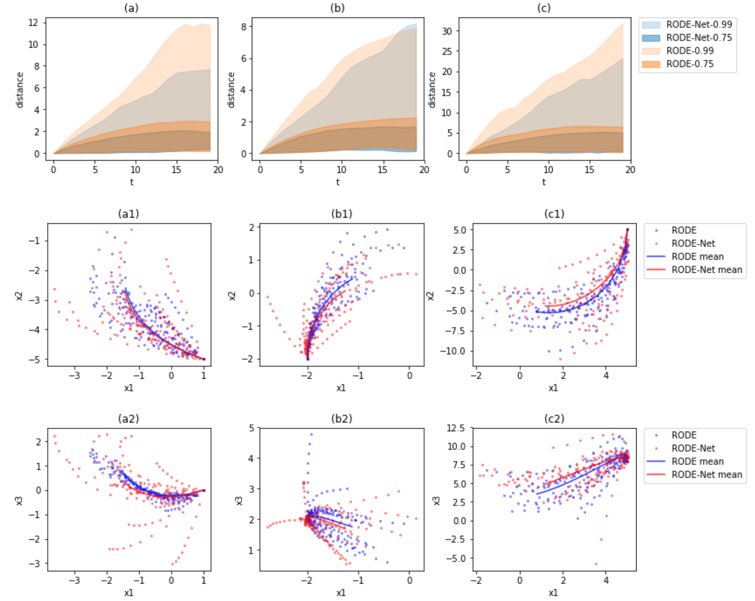
Figure 3: The predicted trajectories of the ODEs sampled from RODE-Net and the original RODE.

We also compare the estimated distribution of the parameters from RODE-Net with those of the RODE by calculating the mean and standard deviation of the coefficients from 100 generated ODEs from RODE-Net. The comparisons for the case RODE_ind are shown in Table 1. We can see that the RODE-Net successfully differentiates between the terms with and without randomness. For the terms exist in the RODE, the mean and standard deviation estimated by the RODE-Net is close to those of the RODE, while the estimated coefficients that do not exist in the RODE have relatively small means and standard deviations.

Table 1: The mean and standard deviation of the estimated coefficients for RODE_ind.

term	coefficients of $\frac{dx_{1}}{dt}$		coefficients of $\frac{dx_{2}}{dt}$		coefficients of $\frac{dx_{3}}{dt}$
	RODE-Net	RODE_ind	RODE-Net	RODE_ind	RODE-Net	RODE_ind
1	0.029(0.764)	0	-0.069(0.527)	0	0.075(0.904)	0
$x_{1}$	-1.841(0.921)	-2.000(1.000)	-0.770(1.725)	-1.000(2.000)	0.025(0.414)	0
$x_{2}$	1.729(0.873)	2.000(1.000)	-0.988(0.304)	-1.000(0)	-0.051(0.506)	0
$x_{3}$	-0.002(0.051)	0	-0.007(0.140)	0	-0.904(0.834)	-1.000(1.000)
$x_{1}x_{3}$	-0.035(0.027)	0	-0.805(0.180)	-1.000(0)	-0.003(0.070)	0
$x_{1}^{2}$	0.006(0.058)	0	0.035(0.267)	0	-0.077(0.149)	0
$x_{1}x_{2}$	-0.001(0.065)	0	0.020(0.198)	0	0.799(0.397)	1.000(0)

Table 2: The estimated covariance of the coefficients for RODE_ind and RODE_dep.

	$cov(a,b)$		$cov(a,c)$		$cov(b,c)$
	estimated	true	estimated	true	estimated	true
RODE_ind	0.075	0	-0.019	0	-0.061	0
RODE_dep	-1.659	-2	0.900	1	-1.700	-2

Moreover, we show that RODE-Net can also well identify RODE with a joint distribution of its parameters. Table 2 shows the covariance of the coefficients of 100 ODEs generated from RODE-Net. We use the coefficient of term $x_{2}$ of $\frac{dx_{1}}{dt}$, $x_{1}$ of $\frac{dx_{2}}{dt}$, $-x_{3}$ of $\frac{dx_{3}}{dt}$ to estimate the random coefficients $a,b,c$ in (8). In both cases, the covariance of the coefficients of RODE-Net are close to the true value.

4.3 The Regularization Effect of GAN in RODE-Net

In this subsection, we demonstrate the regularization effect of the trained GAN in improving the estimates of ODE-Nets. We compare the performance of the RODE-Net (i.e. ODE-Nets with GAN regularization trained by Algorithm 1) with the trained ODE-Nets without GAN regularization (trained by warm-up-1 of Algorithm 1) and find that the GAN regularization helps in reducing prediction error and correcting the learned formulas of the ODEs. For convenience, we shall refer to the ODE-Nets without GAN regularization simply as ODE-Nets.

Let $e^{i}_{1}(t)$ (resp. $e^{i}_{2}(t)$) be the median of relative errors of the prediction of the $i$-th sample of the RODE-Net (resp. ODE-Nets) at time $t$ among 100 initial points. We generate in total $500$ instances. Denote the error vectors $\vec{e}_{j}(t)=(e^{1}_{j}(t),\ldots,e^{500}_{j}(t))$ with $j=1,2$. We compare the histograms of $\vec{e}_{1}(t)$ and $\vec{e}_{1}(t)$ at $t=20,30,40,50$ in Fig. 4. For a better visual comparison, we cropped the vectors $\vec{e}_{j}(t)$ within the range $[0.2,2]$. The numbers of ODE instances for the RODE-Net and ODE-Nets with error $<0.2$ are comparable, while the number of ODE instances for RODE-Net is smaller than that of the ODE-Nets with error $>2$.

As one can see that, the GAN regularization of RODE-Net notably improves overall prediction errors in comparison with ODE-Nets. For some ODE instance the improvement can be rather significant. In Fig. 5, we plot the quantiled relative error vectors for a particular instance of the ODE-Nets with and without GAN regularization.

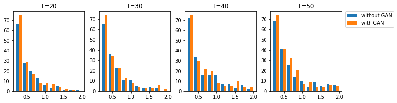
Figure 4: The histogram of the prediction error of the ODE-Nets trained with and without GAN regularization at four time instances.

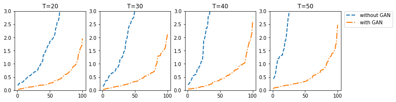
Figure 5: The order statistic of prediction error at four time instances.

GAN regularization in RODE-Net also helps with the estimation of the expression of the RODE. In Fig. 6(a), we compared the distribution of the errors $\vec{e}_{\bm{\eta}}:=\{\|\hat{\bm{\eta}_{i}}-\bm{\eta}_{i}\|_{1}:1\leq i\leq 500\}$ associated to the ODE-Nets with and without GAN regularization. As one can see that, GAN regularization indeed helps with the estimation of the expression of the RODE.

We note that some of the estimations by RODE-Net is notably more accurate than the ODE-Nets without GAN regularization. An example is shown in the table in Fig.6(b). We can see that the estimated coefficients of the primary terms of the ODE are closer to the true values when trained with GAN regularization.

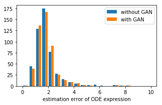
(a)

term	without GAN	with GAN	true
$x_{1}x_{2}$	0.9074	0.9164	1
$1$	0.3755	0.0793	0
$x_{2}$	-0.2055	-0.1316	0
$x_{3}$	-0.2567	-0.1651	-0.143

(b)

   

Figure 6: Left: The histograms of $\vec{e}_{\bm{\eta}}$ of ODE-Nets with and without GAN regularization. the mean and standard deviation of the errors among 500 ODE instances of ODE-Nets with and without GAN regularization are 2.093(3.352) and 2.122(3.372) respectively. Right: The coefficients of $\frac{dx_{3}}{dt}$ in the learned ODE.

5 Conclusion and Future Work

In this paper, we proposed a new framework called RODE-Net to identify RODE from data. The RODE-Net is a combination of ODE-Net for system identification and GAN for parameter distribution estimation. Numerical experiments demonstrated that the trained RODE-Net was able to identify ODEs with minor prior knowledge on the dynamics, but was also able to well estimate the distribution of the RODE. This enabled us to simulate trajectories using the trained RODE-Net that distributed similarly to the ODEs generated from the true RODE. Moreover, the well trained GAN in the RODE-Net served as an effective regularization that enabled the RODE-Net to obtain more accurate predictions and parameter estimations compared to the ODE-Nets without GAN regularization. One limitation and possible further extension of the RODE-Net is that, due to the high dimensionality of the parameters of the ODE-Net, one may include more prior knowledge to reduce the dimension. Furthermore, we would also like to apply the proposed framework to more practical examples, such as the particle fluid systems. It is also worth to study how to design a better data driven regularization based on or beyond GAN.

6 Broader Impact

The proposed RODE-Net differs from earlier works major in twofold and hence it may lead to further impact. 1) The proposed RODE-Net was used to estimate the parameters’ distribution of the RODE rather than the best set of parameters in average sense. While most classical methods focus on uncertainty forward propagation and parameter calibration, the RODE-Net may encourage us to investigate alternative ways to model systems with inherent randomness. 2) The learned GAN was further used as a data driven regularization. This approach can also be generalized to inverse problems of partial differential equations. It is worth exploring on how to use GAN to improve or even replace the commonly used empirical regularization methods. However, due to the non-transparency of deep neural networks, the learned generator of GAN and the corresponding data driven regularization is not always reliable. One should be cautious when deploying GAN based regularization in practice, especially for systems with low fault tolerance.

References

- (1) Zichao Long, Yiping Lu, and Bin Dong. Pde-net 2.0: Learning pdes from data with a numeric-symbolic hybrid deep network. Journal of Computational Physics, page 108925, 2019.
- (2) Zhouchen Lin, Wei Zhang, and Xiaoou Tang. Learning partial differential equations for computer vision. Peking Univ., Chin. Univ. of Hong Kong, 2008.
- (3) Risheng Liu, Zhouchen Lin, Wei Zhang, and Zhixun Su. Learning pdes for image restoration via optimal control. In European Conference on Computer Vision, pages 115–128. Springer, 2010.
- (4) Zichao Long, Yiping Lu, Xianzhong Ma, and Bin Dong. Pde-net: Learning pdes from data. In International Conference on Machine Learning, pages 3214–3222, 2018.
- (5) Ravi G Patel and Olivier Desjardins. Nonlinear integro-differential operator regression with neural networks. arXiv preprint arXiv:1810.08552, 2018.
- (6) Maziar Raissi and George Em Karniadakis. Hidden physics models: Machine learning of nonlinear partial differential equations. Journal of Computational Physics, 357:125–141, 2018.
- (7) Steven L Brunton, Joshua L Proctor, and J Nathan Kutz. Discovering governing equations from data by sparse identification of nonlinear dynamical systems. Proceedings of the National Academy of Sciences, page 201517384, 2016.
- (8) Josh Bongard and Hod Lipson. Automated reverse engineering of nonlinear dynamical systems. Proceedings of the National Academy of Sciences, 104(24):9943–9948, 2007.
- (9) Michael Schmidt and Hod Lipson. Distilling free-form natural laws from experimental data. science, 324(5923):81–85, 2009.
- (10) Hao Xu, Haibin Chang, and Dongxiao Zhang. Dlga-pde: Discovery of pdes with incomplete candidate library via combination of deep learning and genetic algorithm. arXiv preprint arXiv:2001.07305, 2020.
- (11) Ralph C Smith. Uncertainty quantification: theory, implementation, and applications, volume 12. Siam, 2013.
- (12) Wing Kam Liu, Ted Belytschko, and A Mani. Probabilistic finite elements for nonlinear structural dynamics. Computer Methods in Applied Mechanics and Engineering, 56(1):61–81, 1986.
- (13) Dongxiao Zhang. Stochastic methods for flow in porous media: coping with uncertainties. Elsevier, 2001.
- (14) Roger G Ghanem and Pol D Spanos. Stochastic finite elements: a spectral approach. Courier Corporation, 2003.
- (15) Dongbin Xiu. Numerical methods for stochastic computations: a spectral method approach. Princeton university press, 2010.
- (16) Marc C Kennedy and Anthony O’Hagan. Bayesian calibration of computer models. Journal of the Royal Statistical Society: Series B (Statistical Methodology), 63(3):425–464, 2001.
- (17) Xiaoli Chen, Jinqiao Duan, and George Em Karniadakis. Learning and meta-learning of stochastic advection-diffusion-reaction systems from sparse measurements. arXiv preprint arXiv:1910.09098, 2019.
- (18) Liu Yang, Xuhui Meng, and George Em Karniadakis. B-pinns: Bayesian physics-informed neural networks for forward and inverse pde problems with noisy data. arXiv preprint arXiv:2003.06097, 2020.
- (19) Liu Yang, Dongkun Zhang, and George Em Karniadakis. Physics-informed generative adversarial networks for stochastic differential equations. SIAM Journal on Scientific Computing, 42(1):A292–A317, 2020.
- (20) Ian Goodfellow, Jean Pouget-Abadie, Mehdi Mirza, Bing Xu, David Warde-Farley, Sherjil Ozair, Aaron Courville, and Yoshua Bengio. Generative adversarial nets. In Advances in neural information processing systems, pages 2672–2680, 2014.
- (21) Martin Arjovsky, Soumith Chintala, and Léon Bottou. Wasserstein generative adversarial networks. In Proceedings of the 34th International Conference on Machine Learning-Volume 70, pages 214–223, 2017.
- (22) Ishaan Gulrajani, Faruk Ahmed, Martin Arjovsky, Vincent Dumoulin, and Aaron C Courville. Improved training of wasserstein gans. In Advances in neural information processing systems, pages 5767–5777, 2017.
- (23) Ashish Bora, Ajil Jalal, Eric Price, and Alexandros G Dimakis. Compressed sensing using generative models. In Proceedings of the 34th International Conference on Machine Learning-Volume 70, pages 537–546. JMLR. org, 2017.
- (24) Viraj Shah and Chinmay Hegde. Solving linear inverse problems using gan priors: An algorithm with provable guarantees. In 2018 IEEE International Conference on Acoustics, Speech and Signal Processing (ICASSP), pages 4609–4613. IEEE, 2018.
- (25) Christian Ledig, Lucas Theis, Ferenc Huszár, Jose Caballero, Andrew Cunningham, Alejandro Acosta, Andrew Aitken, Alykhan Tejani, Johannes Totz, Zehan Wang, et al. Photo-realistic single image super-resolution using a generative adversarial network. In Proceedings of the IEEE conference on computer vision and pattern recognition, pages 4681–4690, 2017.
- (26) Xiaoying Han and Peter E Kloeden. Random ordinary differential equations and their numerical solution. Springer, 2017.
- (27) Tobias Neckel and Florian Rupp. Random differential equations in scientific computing. Walter de Gruyter, 2013.
- (28) Diederik P Kingma and Jimmy Ba. Adam: A method for stochastic optimization. arXiv preprint arXiv:1412.6980, 2014.