A Self Consistent Field Formulation of Excited State Mean Field Theory

Abstract

We show that, as in Hartree Fock theory, the orbitals for excited state mean field theory can be optimized via a self-consistent one-electron equation in which electron-electron repulsion is accounted for through mean field operators. In addition to showing that this excited state ansatz is sufficiently close to a mean field product state to admit a one-electron formulation, this approach brings the orbital optimization speed to within roughly a factor of two of ground state mean field theory. The approach parallels Hartree Fock theory in multiple ways, including the presence of a commutator condition, a one-electron mean-field working equation, and acceleration via direct inversion in the iterative subspace. When combined with a configuration interaction singles Davidson solver for the excitation coefficients, the self consistent field formulation dramatically reduces the cost of the theory compared to previous approaches based on quasi-Newton descent.

I Introduction

Hartree Fock (HF) theory Szabo and Ostlund (1996); Helgaker, Jøgensen, and Olsen (2000) is so immensely useful in large part due to the rigorous and convenient link it provides between a qualitatively correct many-electron description and an affordable and more intuitive one-electron equation. The link it makes is rigorous in that, when solved, its one-electron equation guarantees that the many-electron description underneath it is optimal in a variational sense, meaning that the energy is made stationary with respect to changes in the wave function. The link is also convenient, because many-electron properties like the energy can be evaluated in terms of inexpensive one-electron quantities, and because solving a one-electron equation, even one with mean field operators that must be brought to self-consistency, is in most cases easier and less expensive than a direct minimization of the many-electron energy. The fact that this useful link is possible at all owes much to the simplicity of the Slater determinant many-electron wave function on which HF theory is built. Essentially, the Slater determinant is as close as we can get to a truly mean field, correlation-free Hartree product ansatz while still capturing the important effects of Pauli correlation. Happily, this single step away from a product state does not prevent a useful and intuitive formulation in terms of a self-consistent one-electron equation in which mean field operators account for electron-electron coulomb repulsion.

In this paper, we will show how excited state mean field (ESMF) theory Shea and Neuscamman (2018) can also be formulated in terms of a one-electron mean field equation that, when solved self consistently, produces optimal orbitals. As in HF theory, this formulation is possible thanks to the ansatz hewing closely to the mean field limit: ESMF takes only one additional step away from a truly mean field product state by adding the open-shell correlation that arises in an excitation on top of the Pauli correlations already present in the ground state. Perhaps most importantly, the resulting one-electron equation that determines the optimal orbitals can, like the Roothaan equations, be solved by iteratively updating a set of mean field operators until they are self-consistent with the orbital shapes. As we will see, when accelerated by direct inversion in the iterative subspace (DIIS), Pulay (1982) this self consistent field (SCF) approach brings the orbital optimization cost down to within a factor of two of HF theory, and significantly lowers the overall cost of ESMF theory compared to previous approaches. Given that ESMF offers a powerful platform upon which to construct excited-state-specific correlation theories Zhao and Neuscamman (2020a); Shea, Gwin, and Neuscamman (2020); Clune, Shea, and Neuscamman (2020) and that it has recently been shown to out-compete other low-cost methods like configuration interaction singles (CIS) and density functional theory in the prediction of charge density changes, Zhao and Neuscamman (2020b) this acceleration of the theory and simplification of its implementation should prove broadly useful.

While recent work has provided an improved ability to optimize the ESMF ansatz via the nonlinear minimization of a generalized variational principle (GVP), Shea, Gwin, and Neuscamman (2020); Zhao and Neuscamman (2020b) the current lack of an SCF formulation stands in sharp contrast to the general state of affairs for methods based on Slater determinants. Even in contexts outside of standard HF for ground states, SCF procedures are the norm rather than the exception when it comes to optimizing Slater determinants’ orbitals. Indeed, among many others, the $\Delta$SCF, Bagus (1965); Hsu, Davidson, and Pitzer (1976); Naves de Brito et al. (1991); Besley, Gilbert, and Gill (2009) restricted open-shell Kohn Sham, Filatov and Shaik (1999); Kowalczyk et al. (2013) constrained density functional theory, Wu and Van Voorhis (2005) ensemble density functional theory, Theophilou (1979); Kohn (1986); Gross, Oliveira, and Kohn (1988) projected HF, Jiménez-Hoyos et al. (2012) and $\sigma$-SCF Ye et al. (2017); Ye and Voorhis (2019) methods all favor SCF optimization approaches. Although the direct minimization of a GVP or the norm of the energy gradient Hait and Head-Gordon (2020) offers protection against a Slater determinant’s “variational collapse” to the ground state or lower excited states, this rigorous safety comes at some cost to efficiency. It is not for nothing that direct energy minimization methods, although available, Van Voorhis and Head-Gordon (2002) are not the default HF optimization methods in quantum chemistry codes. In cases where they prove stable, SCF approaches are typically more efficient. In the case of the ESMF anstatz, an SCF approach is also at risk of collapse to an undesired state, but, even in such troublesome cases, a brief relaxation of the orbitals by SCF may still offer a low-cost head start for the direct minimization of a GVP. In cases where an SCF approach to ESMF is stable, history strongly suggests that it will be more efficient than nonlinear minimization. In short, our preliminary data agree with history’s suggestion.

II Theory

II.1 Hartree-Fock Theory

To understand how an SCF formulation of ESMF theory comes about, it is useful to first review the formulation of HF theory and in particular how its condition for optimal orbitals can be written as a commutator between a mean field operator and a one-body reduced density matrix (RDM). In HF theory, the energy of the Slater determinant $\Psi_{SD}$ is made stationary with respect to changes in the orbital variables, which is the Slater determinant’s approximation of the more general condition that an exact energy eigenstate will have an energy that is stationary with respect to any infinitesimal variation in the wave function. For convenience, and without loss of generality, the molecular orbitals are constrained by Lagrange multipliers to be orthonormal. Szabo and Ostlund (1996) For Restricted Hartree Fock (RHF), the resulting Lagrangian

$$L_{RHF} =E_{RHF}+2\hskip 1.42262pt\mathrm{tr}\left[(\bm{I}-\bm{C}^{T}\bm{S}\bm{C})\bm{\epsilon}\right]$$ (1)

in which $\bm{C}$ is the matrix whose columns hold the molecular orbital coefficients, $\bm{S}$ is the atomic orbital overlap matrix, $\bm{I}$ is the identity matrix, $\bm{\epsilon}$ is the symmetric matrix of Lagrange multipliers, $\mathrm{tr}[]$ is the matrix trace operation, and $E_{RHF}$ is the RHF energy (given below), is then made stationary by setting derivatives with respect to $\bm{C}$ equal to zero. After some rearrangement, Szabo and Ostlund (1996) this condition can be formulated into the famous Roothaan equations,

$$\big{(}\bm{h}+\bm{W}\left[\bm{A}\right]\big{)}\bm{C}=\bm{S}\bm{C}\bm{\epsilon}$$ (2)

in which $\bm{h}$ is the matrix representation of the one-electron components of the Hamiltonian in the atomic orbital basis and $\bm{W}$ is interpreted as a mean field approximation for electron-electron repulsions. Of course, this mean field repulsion depends on the orbital shapes, causing the operator $\bm{W}$ to be a function of $\bm{A}$, the Aufbau determinant’s 1-body $\alpha$-spin RDM. In what comes below we will consider RDMs and other matrices in both the atomic orbital (AO) and molecular orbital (MO) bases, and will adopt the notation that a matrix with no superscript (e.g. $\bm{A}$) refers to the AO representation, while the MO representation is explicitly denoted as such (e.g. $\bm{A}^{(MO)}$). The closed-shell Aufbau determinant’s RDM has the form

$$\bm{A}^{(MO)}=\bm{I}_{o}\qquad\bm{A}=\bm{C}\bm{A}^{(MO)}\bm{C}^{T}$$ (3)

where the matrix $\bm{I}_{o}$ has ones on the first $n_{o}$ elements of its diagonal and zeros elsewhere ($n_{o}$ is the number of occupied molecular orbitals). Although in many contexts it is useful to separate the restricted HF (RHF) mean field electron-electron repulsion operator $\bm{W}[\bm{A}]=2\bm{J}[\bm{A}]-\bm{K}[\bm{A}]$ into its “coulomb” $\bm{J}$ and “exchange” $\bm{K}$ components,

$$J[\mathcal{\gamma}]_{pq} =\sum_{rs}{\mathcal{\gamma}_{rs}(rs|pq)}$$ (4)

$$K[\mathcal{\gamma}]_{pq} =\sum_{rs}{\mathcal{\gamma}_{rs}(pr|qs)},$$ (5)

defined here using the two-electron integrals in 1122 order, this separation is not necessary at present and so we will work instead in terms of the combined mean field operator $\bm{W}$.

Now, while the Roothaan equation has both an intuitive appeal as a one-electron Schrödinger equation and a practical appeal as a convenient setup for an SCF cycle based on the efficient numerical diagonalization of a symmetric generalized eigenvalue problem, it is not the only way to formulate HF theory’s central requirement of Lagrangian stationarity. Noting that only the first $n_{o}$ columns of $\bm{C}$ affect the ansatz, we can right-multiply Eq. (2) by $\bm{I}_{o}=\bm{A}^{(MO)}$ to focus our attention on them while at the same time left-multiplying by $\bm{C}^{T}$ to eliminate the overlap matrix, which results in

$$\bm{F}^{(MO)}\bm{A}^{(MO)}=\bm{C}^{T}\big{(}\bm{h}+\bm{W}\big{)}\bm{C}\bm{A}^{(MO)}=\bm{\epsilon}\bm{I}_{o}$$ (6)

where we have made the usual definition of the Fock operator.

$$\bm{F}^{(MO)}=\bm{C}^{T}\bm{F}\bm{C}=\bm{C}^{T}\big{(}\bm{h}+\bm{W}\big{)}\bm{C}$$ (7)

If we ensure that we work in the canonical representation, Szabo and Ostlund (1996) the matrix $\bm{\epsilon}$ will be diagonal, and so Eq. (6) essentially says that the product $\bm{F}^{(MO)}\hskip 0.85358pt\bm{A}^{(MO)}$ must produce a symmetric matrix. We may enforce this requirement by setting the difference between this product and its transpose equal to zero, which leads to a commutator condition for Lagrangian stationarity that can be used as an alternative to the Roothaan equation when optimizing orbitals. McWeeny (1996); Pulay (1982)

$$\big{[}\hskip 1.70717pt\bm{C}^{T}\bm{F}\bm{C},\hskip 1.70717pt\bm{A}^{(MO)}\hskip 1.70717pt\big{]}=0$$ (8)

If we consider the HF energy expression

$$E_{RHF}=\mathrm{tr}\big{[}(2\bm{h}+\bm{W})\bm{A}\big{]}$$ (9)

alongside the Fock operator definition $\bm{F}=\bm{h}+\bm{W}$, we see a nice connection between the commutator condition and the energy. Specifically, if one halves the one-electron component of the mean field operator whose trace with the density yields the energy, the resulting operator ($\bm{F}$ in this case) must, when put in the MO basis, commute with the MO basis representation of the density matrix in order for the Lagrangian to be stationary. With this connection pointed out, we now turn our attention to ESMF theory, where a generalization of Eq. (8) yields a useful SCF formulation for orbital optimization.

II.2 Excited State Mean Field Theory

Like HF theory, the energy expression for the ESMF ansatz for a singlet excited state can be written in terms of traces between mean field operators and density-like matrices. In particular, if we take the simple version of the singlet ESMF ansatz in which the Aufbau coefficient is set to zero,

$$\left.|\Psi_{ESMF}\right\rangle=\sum_{ia}t_{ia}\left|\hskip 0.85358pt{}^{a_{\uparrow}}_{i_{\uparrow}}\right\rangle+t_{ia}\left|\hskip 0.85358pt{}^{a_{\downarrow}}_{i_{\downarrow}}\right\rangle,$$ (10)

where $\bm{t}$ is the matrix of CIS-like configuration interaction coefficients and $\left|\hskip 0.85358pt{}^{a\uparrow}_{i\uparrow}\right\rangle$ is the Slater determinant resulting from an $\hskip 2.84526pti\rightarrow a\hskip 2.84526pt$ $\alpha$-spin excitation out of the Aufbau determinant (note we do not say the HF determinant, as we are not in the HF MO basis), then the ESMF singlet energy amounts to four traces between mean field operators and density-like matrices.

$$E_{ESMF}=\hphantom{+}\hskip 1.42262pt\mathrm{tr}\big{[} \hskip 1.99168pt(\hskip 1.42262pt2\bm{h}\hskip 0.85358pt+\bm{W}[\bm{A}]\hskip 1.99168pt)\hskip 2.84526pt\mathcal{\gamma}\hskip 2.84526pt\big{]}+\hskip 1.42262pt\mathrm{tr}\big{[}\hskip 1.42262pt\bm{W}[\bm{D}]\hskip 1.42262pt\bm{A}\hskip 1.42262pt\big{]}$$

$$+\hskip 1.42262pt\mathrm{tr}\big{[} \hskip 1.42262pt\bm{W}[\bm{T}]\hskip 1.42262pt\bm{T}^{T}\hskip 1.42262pt\big{]}+\hskip 1.42262pt\mathrm{tr}\big{[}\hskip 1.42262pt(\bm{W}[\bm{T}])^{T}\hskip 1.42262pt\bm{T}\hskip 1.42262pt\big{]}$$ (11)

Here $\mathcal{\gamma}$ is the one-body alpha-spin RDM for the ESMF ansatz.

$$\gamma^{(MO)}=\bm{I}_{o}+\left(\begin{array}[]{c|c}-\bm{t}\hskip 1.13809pt\bm{t}^{T}&0\\ \hline\cr 0&\bm{t}^{T}\bm{t}\rule{0.0pt}{10.81204pt}\end{array}\right)\qquad\gamma=\bm{C}\gamma^{(MO)}\bm{C}^{T}$$ (14)

The matrix $\bm{A}$ is the Aufbau determinant’s one-body RDM, as in Eq. (3). The difference between these density matrices we define as $\bm{D}=\gamma-\bm{A}$. Finally, $\bm{T}$ is the non-symmetric matrix that, in its MO representation, has the $\alpha$-spin transition density matrix between the Aufbau determinant and the ESMF ansatz (which is as for CIS just $\bm{t}\hskip 0.56905pt$) in its upper-right corner.

$$\bm{T}^{(MO)}=\left(\begin{array}[]{c|c}0&\bm{t}\\ \hline\cr 0&0\rule{0.0pt}{10.81204pt}\end{array}\right)\qquad\bm{T}=\bm{C}\bm{T}^{(MO)}\bm{C}^{T}$$ (17)

With the ESMF energy written in terms of one-body mean field operators and density-like matrices, we can now present our central result, in which the stationarity conditions for the ESMF Lagrangian

$$L_{ESMF}=E_{ESMF}+2\hskip 1.42262pt\mathrm{tr}\left[(\bm{I}-\bm{C}^{T}\bm{S}\bm{C})\bm{\epsilon}\right]$$ (18)

with respect to orbital variations are written in a one-electron equation that admits an SCF-style solution. We begin, as in HF theory, by setting the (somewhat messy) derivatives $\partial L_{ESMF}/\partial\bm{C}$ equal to zero. With some care, this condition can be organized into

$$\big{(}\bm{h}+\bm{W}[\bm{A}]\big{)}C\gamma^{(MO)}+\bm{W}[\bm{D}]CA^{(MO)}$$

$$\hskip 17.07164pt+\bm{W}[\bm{T}]C(T^{(MO)})^{T}+(\bm{W}[\bm{T}])^{T}CT^{(MO)}=\bm{S}\bm{C}\bm{\epsilon}$$ (19)

whose structure is similar to but also notably different from the analogous HF expression in Eq. (2). The formal difference is that there are now four terms on the left hand side, one for each trace in the energy expression. The practical difference is that the ESMF equation is not an eigenvalue problem, and it is not obvious that it can be reorganized into one due to the incompatible kernels of the matrices $\gamma^{(MO)}$, $A^{(MO)}$, and $T^{(MO)}$. Thus, it is at present not clear whether this ESMF equation can offer the same spectral information that the Roothaan equation provides for HF. Nonetheless, for orbital optimization, we have found a convenient alternative by transforming this stationary condition into commutator form by following the same steps that took us from Eq. (2) to Eq. (8) in HF theory. Defining $\bm{F}_{A}=\bm{h}+\bm{W}[\bm{A}]$, the result is that the Lagrangian stationary condition can be written as

$$0= \hskip 0.85358pt\big{[}\hskip 2.84526pt\bm{C}^{T}\bm{F}_{A}\bm{C},\hskip 2.84526pt\mathcal{\gamma}^{(MO)}\hskip 2.84526pt\big{]}$$

$$+\big{[}\hskip 2.84526pt\bm{C}^{T}\bm{W}[\bm{D}]\bm{C},\hskip 2.84526pt\bm{A}^{(MO)}\hskip 2.84526pt\big{]}$$

$$+\big{[}\hskip 2.84526pt\bm{C}^{T}\bm{W}[\bm{T}]\bm{C},\hskip 2.84526pt(\bm{T}^{(MO)})^{T}\hskip 2.84526pt\big{]}$$

$$+\big{[}\hskip 2.84526pt\bm{C}^{T}(\bm{W}[\bm{T}])^{T}\bm{C},\hskip 2.84526pt\bm{T}^{(MO)}\hskip 2.84526pt\big{]}.$$ (20)

It is interesting that the same pattern holds as in the HF case: the commutator condition has one commutator per trace in the energy expression, and the mean field operators (with any one-electron parts halved) are again paired with the same density-like matrices as in the energy traces. We find this pattern especially interesting in light of the fact that it does not simply follow that each trace produces one commutator. Instead, cancellations of terms coming from derivatives on different traces are needed to arrive at the commutators above, and so we do wonder whether this is a happy accident or whether there is an underlying reason to expect such cancellations.

II.3 Self Consistent Solution

Either way, Eq. (20) forms the basis for an efficient SCF optimization of the ESMF orbitals. Assuming that we are a small orbital rotation away from stationarity, we insert the rotation $\bm{C}\rightarrow\bm{C}\mathrm{exp}(\bm{X})$ into our commutator condition and then expand the exponential and drop all terms higher than linear order in the anti-symmetric matrix $\bm{X}$. The result is a linear equation for $\bm{X}$ (see Eq. (S26) in the Supplementary Material) which we solve via the iterative GMRES method. Note that, if desired, one can control the maximum step size in $\bm{X}$ by simply stopping the GMRES iterations early if the norm of $\bm{X}$ grows beyond a user-supplied threshold. This may be desirable, as we did after all assume that only a small rotation was needed and our linearization of the equation prevents us from trusting any proposed rotation that is large in magnitude. In parallel to SCF HF theory, which holds $\bm{F}$ fixed while solving the Roothaan equation for new orbitals, we hold $\bm{F}_{A}$, $\bm{W}[\bm{D}]$, and $\bm{W}[\bm{T}]$ fixed while solving our linear equation. Thus, although the modified GMRES solver is not as efficient as the dense eigenvalue solvers used for HF theory, it remains relatively inexpensive as it does not does not involve any Fock builds and so does not have to access the two-electron integrals. (Technical note: in practice, we can speed up the GMRES solver considerably by preconditioning it with a diagonal approximation to the linear transformation that is set to one for $\bm{X}$ elements in the occupied-occupied and virtual-virtual blocks (since these are expected to play little role in the orbital relaxation) and, in the other blocks, replaces $\bm{C}^{T}\bm{F}_{A}\bm{C}$ with its diagonal, replaces $\gamma^{(MO)}$ with $\bm{I}_{o}$, and neglects $\bm{W}[\bm{D}]$ and $\bm{W}[\bm{T}]$ (see Supplementary Material for the explicit form). DIIS is also effective when we take Eq. (20) transformed into the AO basis as the error vector and the $\bm{F}_{A}$, $\bm{W}[\bm{D}]$ and $\bm{W}[\bm{T}]$ matrices as the DIIS parameters. We use both of these accelerations in all calculations.) Only after the linear equation is solved and the orbitals are updated do we rebuild the three mean field operators, and so each overall SCF iteration requires just three Fock builds, which, as they can be done during the same loop over the two-electron integrals, come at a cost that is not much different than HF theory’s single Fock build. This arrangement contrasts sharply with the nine Fock builds and two integral loops that are necessary to form the analytic derivative of the energy with respect to $\bm{C}$ that is used in descent-based orbital optimization. Zhao and Neuscamman (2020b) In summary, the ESMF orbitals, like the HF orbitals, can be optimized particularly efficiently via the self-consistent solution of a one-electron mean field equation.

Although this exciting result makes clear that the ESMF ansatz really does hew closely enough to the mean field product-state limit for one-electron mathematics to be of use, there are a number of questions we should now address. First, and we will go into more detail on this point in the next paragraph, is the SCF approach actually faster than descent? The answer, at least in simple systems, is a resounding yes. Second, what of the configuration interaction coefficients $\bm{t}$? At present, we optimize them in a two-step approach, in which we go back and forth between orbital SCF solutions and CIS calculations (taking care to include the new terms that arise for CIS when not in the HF MO basis) until the energy stops changing. In future, more sophisticated approaches that provide approximate coupling between these optimizations may be possible, as has long been true in multi-reference theory. Kreplin, Knowles, and Werner (2020) Third, what physical roles can we ascribe to the different mean field operators that appear in the SCF approach to ESMF? The operator $\bm{F}_{A}$ obviously carries the lion’s share of the electron-electron repulsion, as it is the only mean field operator derived from a many-electron density matrix. Indeed, $\bm{W}[\bm{D}]$ and $\bm{W}[\bm{T}]$ represent repulsion from one-electron densities, and so they cannot provide the bulk of the electron-electron repulsion. Thus, we suggest that it is useful to view $\bm{F}_{A}$ as a good starting point that includes the various repulsions between electrons not involved in the excitation but that gets the repulsions affected by the excitation wrong. $\bm{W}[\bm{D}]$ and $\bm{W}[\bm{T}]$ then act as single-electron-density corrections to this starting point. If one considers the simple case in which we ignore all electrons other than the pair involved in the excitation (e.g. consider the HOMO/LUMO excitation in H₂), then a close inspection reveals that $\bm{W}[\bm{D}]$ eliminates the spurious HOMO-HOMO repulsion that is present in the first trace of the energy expression, while the $\bm{W}[\bm{T}]$ terms bring the excited electron pair’s repulsion energy into alignment with the actual repulsion energy that results from the singlet’s equal superposition of two open-shell determinants.

Table 1: Convergence of SCF- and GVP-based ESMF for the HOMO/LUMO excitation of cc-pVDZ H₂O. Initial values for $\bm{t}$ and $\bm{C}$ are set to the two-determinant HOMO/LUMO open shell singlet and the RHF orbitals, respectively. For SCF, the two-step method toggled between CIS and SCF calculations, with CIS going first. As the guess is quite good in this system, the GVP optimization set $\mu=0$ right away and so amounted to a BFGS minimization of the energy gradient norm. At various points during each optimization (measured both by the cumulative number of loops over the TEIs and by the wall time) we report the energy error $\Delta E$ compared to the fully converged energy. Both calculations used a single core on a 2015 MacBook Air.

SCF ESMF				GVP ESMF
TEI Loops	Time (s)	$\Delta E$ (a.u.)		TEI Loops	Time (s)	$\Delta E$ (a.u.)
10	0.007	0.062605		76	0.397	0.003761
20	0.025	0.000032		150	0.783	0.000654
30	0.033	0.000004		226	1.187	0.000184
40	0.054	0.000000		300	1.579	0.000001

Table 2: Total time in seconds and number of iterations $n_{i}$ taken for the orbital optimization in the ground state (for RHF) or the excited state (for SCF-based ESMF) to get within 5$\mu$E_h of its fully converged value. The RHF and ESMF methods rely on the same underlying Fock build code, both use DIIS, and both used one core on a 2015 MacBook Air. For ESMF, only the orbitals are optimized, with $\bm{t}$ set to the HOMO/LUMO open-shell singlet and the initial guess for $\bm{C}$ set to the RHF orbitals. For RHF, the eigen-orbitals of the one-electron Hamiltonian were used as the initial guess for $\bm{C}$. Times do not include the generation of one- and two-electron AO integrals, which are the same for both methods.

Molecule	Basis	RHF (s)	$n_{i}$	ESMF (s)	$n_{i}$
water	cc-pVTZ	0.087	8	0.185	6
formaldehyde	cc-pVTZ	0.424	11	0.862	8
ethylene	cc-pVTZ	0.903	8	1.735	6
toluene	cc-pVDZ	4.366	19	6.835	11

III Results

III.1 Efficiency Comparisons

Returning now to the question of practical efficiency, we report in Table 1 the convergence of the energy for the HOMO/LUMO excitation in the water molecule for both SCF-based and GVP descent-based ESMF (note all geometries can be found in the Supplementary Material). Whether one measures by the number of times the expensive two-electron integral (TEI) access must be performed or by the wall time, the two-step SCF approach is dramatically more efficient than GVP-based descent in this case. (The keen-eyed observer will notice that in the SCF case, the TEI loop count and the wall time do not increase at the same rate, which is due to the CIS iterations having many fewer matrix operations to do as compared to SCF in between each access of the TEIs.) If we focus in on just the orbital optimization, as shown in Table 2, we find that the SCF approach for ESMF is almost as efficient as ground state HF theory. In practice, of course, we also want to optimize $\bm{t}$, and for now we rely on the two-step approach, as used in Table 1.

While the SCF approach has clear advantages in simple cases, the GVP is still expected to be essential for cases in which the SCF approach may not be stable. For example, without implementing an interior root solver or freezing an open core (and we have not done either), Davidson-based CIS would be problematic for a core excitation. However, as shown in Table 3, a combination of an initial SCF optimization of the orbitals followed by a full GVP optimization of $\bm{t}$ and $\bm{C}$ together is quite effective. In this case, the SCF approach brings the energy close to its final value, converging to an energy that is too low by 54 $\mu$E_h (remember, excited states do not have any upper bound guarantee, even when a variational principle like energy stationarity or the GVP is in use). From this excellent starting point, the GVP’s combined optimization of $\bm{C}$ and $\bm{t}$ converges quickly to the final energy, needing just ten gradient evaluations to get within 1 $\mu$E_h. In contrast, if the initial SCF orbital optimization is omitted, the GVP coupled optimization requires hundreds of gradient evaluations (exactly how many depends on the choice for $\omega$ and how $\mu$ is stepped down to zero) Shea, Gwin, and Neuscamman (2020) to reach the same level of convergence, and was only able to converge to the correct state at all by setting $\mu$ to 0.5 and $\omega$ 0.08 E_h lower than the final energy for the initial iterations to avoid converging to a higher-energy core excitation. Especially interesting is the fact that, if we move to the aug-cc-pVTZ basis, the ESMF predictions for the two lowest core excitations in H₂O are 534.3 and 536.2 eV, which are quite close to the experimental values Schirmer et al. (1993) of 534.0 and 535.9 eV and which match the delta between them even more closely. Thus, even in cases where the SCF approach would be difficult to use on its own, it can offer significant benefits in partnership with direct minimization.

Table 3: Convergence of the energy for the lowest singlet core excited state of H₂O in the aug-cc-pVDZ basis. Initial values for $\bm{t}$ and $\bm{C}$ are set to the two-determinant 1s$\rightarrow$LUMO open shell singlet and the RHF orbitals, respectively. An initial SCF optimization converged after 10 iterations (involving one TEI loop each), after which GVP-based BFGS descent (again with $\mu$ set immediately to zero) was started from the SCF result (the GVP requires 2 TEI loops per gradient evaluation). We report the energy error $\Delta E$ compared to the fully converged energy as a function of the cumulative wall time and the cumulative number of TEI loops. The calculation used a single core on a 2015 MacBook Air.

TEI Loops	Time (s)	$\Delta E$ (a.u.)
Start with SCF:
5	0.163	0.008698
10	0.267	-0.000054
Switch to GVP:
20	0.435	0.000002
30	0.604	0.000001

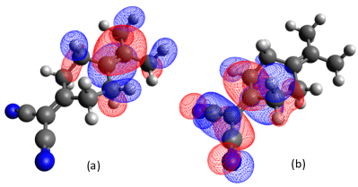
Figure 1: Donor (a) and acceptor (b) orbitals for the lowest charge transfer state in the PYCM molecule as predicted by ESMF. The excited state SCF calculation took just two and a half times as long as the RHF calculation.

III.2 PYCM

To verify that the benefits of the SCF approach are not confined to smaller molecules, we exhibit its use on a charge transfer state in the PYCM molecule that Subotnik used to demonstrate CIS’s bias against charge transfer states. Subotnik (2011) Working in a cc-pVDZ basis for the heavy atoms and 6-31G for hydrogen, we consider the lowest charge transfer state, for which we provide iteration-by-iteration convergence details in the Supplementary Material. In Figure 1, we plot the ESMF prediction for the donor and acceptor orbitals, which in this case are just the relaxed HOMO and LUMO orbitals as the $\bm{t}$ matrix coefficients are strongly dominated by the HOMO$\rightarrow$LUMO transition. We see that this state transfers charge from the $\pi$ bonding orbital on the methylated ethylene moiety to the $\pi^{*}$ orbital on the cyano-substituted ethylene moiety. Aside from the efficiency of the SCF solver in this case (it takes just two-and-a-half times as long as RHF when using the same Fock build code) it is interesting to compare the prediction against that of CIS, which is the analogous theory when orbital relaxation is ignored. CIS predicts a 7.30 eV excitation energy for the lowest state in which this charge transfer transition plays a significant role, whereas ESMF predicts a 4.82 eV excitation energy. This multiple-eV energy lowering after orbital relaxation serves as a stark reminder of how important these relaxations are for charge transfer states.

IV Conclusion

In conclusion, orbital optimization in ESMF theory can be formulated in terms of a one-electron equation in which mean field operators provide electron-electron repulsion and which is brought to self-consistency through an efficient iterative process that closely mirrors ground state HF theory. In particular, it is possible to formulate the excited state many-electron energy in terms of four traces between density matrices and mean field operators, and the central commutator condition likewise contains four commutators between these density matrices and their partner mean field operators. In a sense, this is a straightforward extension of the HF case, where only one trace and one commutator are needed. As has long been true for Slater determinants, the SCF approach to the ESMF orbitals appears to be significantly more efficient than quasi-Newton methods, at least in cases where the SCF iteration converges stably to the desired state. Looking forward, it will be interesting to see if, as in the ground state case, the SCF approach admits Kohn-Sham-style density functionals and whether the optimization of the excitation coefficients can be more tightly coupled to the optimization of the orbitals.

SUPPLEMENTARY MATERIAL

See supplementary material for additional mathematical details, additional calculation details, and molecular geometries.

ACKNOWLEDGEMENTS

This work was supported by the Early Career Research Program of the Office of Science, Office of Basic Energy Sciences, the U.S. Department of Energy, grant No. DE-SC0017869. While final timing calculations were carried out on a laptop, many preliminary calculations with earlier pilot code were performed using the Berkeley Research Computing Savio cluster.

Data Availability Statement — The data that supports the findings of this study are available within the article and its supplementary material.

Appendix A Mathematical Detail

First, let’s rewrite the ESMF ansatz in Eq. (10) as

$$|\Psi_{ESMF}\rangle=\sum_{ia}t_{ia}a^{\dagger}_{\uparrow}i_{\uparrow}|\Phi_{A}\rangle+t_{ia}a^{\dagger}_{\downarrow}i_{\downarrow}|\Phi_{A}\rangle$$ (S1)

where $\Phi_{A}$ refers to the Aufbau determinant and $a^{\dagger}_{\uparrow}$ and $i^{\dagger}_{\uparrow}$ are $\uparrow$-spin creation operators for virtual and occupied orbitals, respectively, in the ESMF molecular orbital basis. We define the Hamiltonian in chemist’s notation as

$$\hat{H}= \hphantom{+}\sum_{pq}h^{(MO)}_{pq}\big{(}\hskip 1.42262ptp^{\dagger}_{\uparrow}q_{\uparrow}\hskip 1.42262pt+\hskip 1.42262ptp^{\dagger}_{\downarrow}q_{\downarrow}\hskip 1.42262pt\big{)}$$

$$+\frac{1}{2}\sum_{pqrs}\{pq|rs\}\big{(}\hskip 2.84526ptp^{\dagger}_{\uparrow}r^{\dagger}_{\uparrow}s_{\uparrow}q_{\uparrow}\hskip 1.42262pt+\hskip 1.42262ptp^{\dagger}_{\downarrow}r^{\dagger}_{\downarrow}s_{\downarrow}q_{\downarrow}$$

$$\hskip 68.2866pt+\hskip 1.42262ptp^{\dagger}_{\uparrow}r^{\dagger}_{\downarrow}s_{\downarrow}q_{\uparrow}\hskip 1.42262pt+\hskip 1.42262ptp^{\dagger}_{\downarrow}r^{\dagger}_{\uparrow}s_{\uparrow}q_{\downarrow}\hskip 2.84526pt\big{)}$$ (S2)

where $\bm{h}^{(MO)}$ and $\{pq|rs\}$ are the one- and two-electron integrals in the ESMF orbital basis. The ESMF energy is

$$E_{ESMF}=\langle\Psi_{ESMF}|\hat{H}|\Psi_{ESMF}\rangle.$$ (S3)

From here on out, we adopt a summation convention in which a sum is implied over any index that appears more than once in the same term. Using this convention, and working through the second-quantized algebra, the ESMF energy becomes

$$E_{ESMF}= \hphantom{+}2\hskip 2.84526ptt_{ia}t_{ib}h^{(MO)}_{ab}-2\hskip 2.84526ptt_{ia}t_{ja}h^{(MO)}_{ij}+4\hskip 2.84526ptt_{ia}t_{ia}h^{(MO)}_{kk}$$

$$+4\hskip 2.84526ptt_{ia}t_{ib}\{ab|kk\}-2\hskip 2.84526ptt_{ia}t_{ib}\{ak|bk\}$$

$$-4\hskip 2.84526ptt_{ia}t_{ja}\{ij|kk\}+2\hskip 2.84526ptt_{ia}t_{ja}\{ik|jk\}$$

$$+4\hskip 2.84526ptt_{ia}t_{ia}\{kk|ll\}-2\hskip 2.84526ptt_{ia}t_{ia}\{kl|kl\}$$

$$+4\hskip 2.84526ptt_{ia}t_{jb}\{ia|jb\}-2\hskip 2.84526ptt_{ia}t_{jb}\{ij|ab\}$$ (S4)

where $a,b,c,d$ are virtual orbitals, $i,j,k,l,m$ are occupied orbitals, and we will use $p,q,r,s,w,x,y,z$ for general orbitals. Note the pattern in the terms: first, the one electron integrals are contracted and summed over, then the two electron integrals. The two electron integral terms come in pairs, one part of each pair corresponding to the conventional coulomb operator and the other to the conventional exchange operator. As in RHF theory, the coulomb terms have an extra factor of two compared to the exchange terms, which is what produces the general pattern of $2J-K$ in the final mean field operators.

To derive Eq. (19), we start with the Lagrangian in Eq. (18), take derivatives with respect to the elements of the orbital coefficient matrix $\bm{C}$, and then set these derivatives equal to zero. Derivatives of the Lagrange multiplier term in Eq. (18) lead to the right hand side of Eq. (19) in the same way that they do for the HF Roothaan equation, and so we will not work through them explicitly. For the derivatives of the ESMF energy, we need to remember that the one- and two-electron integrals in the ESMF molecular orbital basis are transformed from the atomic orbital basis as

$$h^{(MO)}_{pq} =C_{rp}h_{rs}C_{sq}$$ (S5)

$$\{pq|rs\} =C_{wp}C_{xq}C_{yr}C_{zs}(wx|yz)$$ (S6)

where $\bm{h}$ and $(wx|yz)$ are the one- and two-electron integrals (again in chemists’ notation) in the atomic orbital basis. Noting that $\bm{C}$ contains an “occupied” block $C^{(o)}$ (the first $n_{o}$ columns) and a “virtual” block $C^{(v)}$ (the remaining columns), we can consider the derivatives with respect to the elements of these blocks separately. As an example, the occupied block derivative of the first two-electron integral term in Eq. (S4) is (here $m$ is an occupied index and $x$ is a general index)

$$\frac{\partial}{\partial C_{xm}}\bigg{(}t_{ia}t_{ib}\{ab|kk\}\bigg{)}= \hphantom{+}2\hskip 2.84526ptt_{ia}t_{ib}C_{pa}C_{qb}C_{sm}(pq|xs).$$ (S7)

The analogous virtual block derivative is

$$\frac{\partial}{\partial C_{xc}}\bigg{(}t_{ia}t_{ib}\{ab|kk\}\bigg{)}=2\hskip 2.84526ptt_{ic}t_{ia}C_{qa}C_{rk}C_{sk}(xq|rs).$$ (S8)

We now define

$$\mathcal{A}^{coul}_{pq} =\hskip 2.84526ptC_{rk}C_{sk}(pq|rs)$$ (S9)

$$\mathcal{B}^{coul}_{pq} =\hskip 2.84526ptC_{sb}t_{ib}t_{ia}C_{ra}(pq|rs)$$ (S10)

$$\mathcal{C}^{coul}_{pq} =\hskip 2.84526ptC_{ri}t_{ia}t_{ja}C_{sj}(pq|rs)$$ (S11)

$$\mathcal{D}^{coul}_{pq} =\hskip 2.84526ptC_{ri}t_{ia}C_{sa}(pq|rs)$$ (S12)

as well as $\mathcal{A}^{exch}$, $\mathcal{B}^{exch}$, $\mathcal{C}^{exch}$, and $\mathcal{D}^{exch}$, which are the same except for having $q$ and $r$ swapped in the two-electron integral. With these definitions, we can combine Eqs. (S7) and (S8) and write the derivative in matrix form.

$$\frac{\partial}{\partial\bm{C}}\bigg{(}t_{ia}t_{ib}\{ab|kk\}\bigg{)}= \bigg{[}\hskip 2.84526pt2\hskip 2.84526pt\mathcal{B}^{coul}\bm{C}^{(o)}\hskip 5.69054pt\bigg{|}\hskip 5.69054pt\bm{0}\hskip 2.84526pt\bigg{]}$$

$$\hskip 5.69054pt+\bigg{[}\hskip 2.84526pt\bm{0}\hskip 5.69054pt\bigg{|}\hskip 5.69054pt2\hskip 2.84526pt\mathcal{A}^{coul}\bm{C}^{(v)}\bm{t}^{T}\bm{t}\hskip 2.84526pt\bigg{]}$$ (S13)

where on the right hand side we have placed a vertical bar to separate the occupied and virtual blocks of the matrices. Note that we have kept the two matrices on the right hand side here separate, as they will end up contributing to different terms within Eq. (19), which we enumerate as follows.

$$\mathrm{Term~{}1} \quad\big{(}\bm{h}+\bm{W}[\bm{A}]\big{)}C\gamma^{(MO)}$$ (S14)

$$\mathrm{Term~{}2} \quad\bm{W}[\bm{D}]CA^{(MO)}$$ (S15)

$$\mathrm{Term~{}3} \quad\bm{W}[\bm{T}]C(T^{(MO)})^{T}$$ (S16)

$$\mathrm{Term~{}4} \quad(\bm{W}[\bm{T}])^{T}CT^{(MO)}$$ (S17)

We will explicitly work through to Terms 1 and 2. Terms 3 and 4 are derived similarly. Now, each of the first nine terms in Eq. (S4) makes a contribution to Terms 1 or 2. We have already worked out the $\bm{C}$-derivatives for one of these terms (the fourth one) in Eq. (S13). All the others are listed here. Note that the last two derivatives do not make a contribution to Terms 1 or 2, but are listed for completeness.

$$\frac{\partial}{\partial\bm{C}}\bigg{(}t_{ia}t_{ib}h^{(MO)}_{ab}\bigg{)}= \hskip 2.84526pt\bigg{[}\hskip 2.84526pt\bm{0}\hskip 5.69054pt\bigg{|}\hskip 5.69054pt2\hskip 2.84526pt\bm{h}\hskip 1.42262pt\bm{C}^{(v)}\bm{t}^{T}\bm{t}\hskip 2.84526pt\bigg{]}$$

$$\frac{\partial}{\partial\bm{C}}\bigg{(}t_{ia}t_{ja}h^{(MO)}_{ij}\bigg{)}= \hskip 2.84526pt\bigg{[}\hskip 2.84526pt2\hskip 2.84526pt\bm{h}\hskip 1.42262pt\bm{C}^{(o)}\bm{t}\hskip 1.42262pt\bm{t}^{T}\hskip 5.69054pt\bigg{|}\hskip 5.69054pt\bm{0}\hskip 2.84526pt\bigg{]}$$

$$\frac{\partial}{\partial\bm{C}}\bigg{(}t_{ia}t_{ia}h^{(MO)}_{kk}\bigg{)}= \hskip 2.84526pt\bigg{[}\hskip 2.84526pt\hskip 2.84526pt\bm{h}\hskip 1.42262pt\hskip 2.84526pt\bm{C}^{(o)}\hskip 5.69054pt\bigg{|}\hskip 5.69054pt\bm{0}\hskip 2.84526pt\bigg{]}$$

$$\frac{\partial}{\partial\bm{C}}\bigg{(}t_{ia}t_{ib}\{ak|bk\}\bigg{)}= \hskip 2.84526pt\bigg{[}\hskip 2.84526pt2\hskip 2.84526pt\mathcal{B}^{exch}\bm{C}^{(o)}\hskip 5.69054pt\bigg{|}\hskip 5.69054pt\bm{0}\hskip 2.84526pt\bigg{]}$$

$$\hskip 11.38109pt+\hskip 2.84526pt\bigg{[}\hskip 2.84526pt\bm{0}\hskip 5.69054pt\bigg{|}\hskip 5.69054pt2\hskip 2.84526pt\mathcal{A}^{exch}\bm{C}^{(v)}\bm{t}^{T}\bm{t}\hskip 2.84526pt\bigg{]}$$

$$\frac{\partial}{\partial\bm{C}}\bigg{(}t_{ia}t_{ja}\{ij|kk\}\bigg{)}= \hskip 2.84526pt\bigg{[}\hskip 2.84526pt2\hskip 2.84526pt\mathcal{C}^{coul}\bm{C}^{(o)}\hskip 5.69054pt\bigg{|}\hskip 5.69054pt\bm{0}\hskip 2.84526pt\bigg{]}$$

$$\hskip 11.38109pt+\bigg{[}\hskip 2.84526pt2\hskip 2.84526pt\mathcal{A}^{coul}\bm{C}^{(o)}\bm{t}\hskip 1.42262pt\bm{t}^{T}\hskip 5.69054pt\bigg{|}\hskip 5.69054pt\bm{0}\hskip 2.84526pt\bigg{]}$$

$$\frac{\partial}{\partial\bm{C}}\bigg{(}t_{ia}t_{ja}\{ik|jk\}\bigg{)}= \hskip 2.84526pt\bigg{[}\hskip 2.84526pt2\hskip 2.84526pt\mathcal{C}^{exch}\bm{C}^{(o)}\hskip 5.69054pt\bigg{|}\hskip 5.69054pt\bm{0}\hskip 2.84526pt\bigg{]}$$

$$\hskip 11.38109pt+\bigg{[}\hskip 2.84526pt2\hskip 2.84526pt\mathcal{A}^{exch}\bm{C}^{(o)}\bm{t}\hskip 1.42262pt\bm{t}^{T}\hskip 5.69054pt\bigg{|}\hskip 5.69054pt\bm{0}\hskip 2.84526pt\bigg{]}$$

$$\frac{\partial}{\partial\bm{C}}\bigg{(}t_{ia}t_{ia}\{kk|ll\}\bigg{)}= \hskip 2.84526pt\bigg{[}\hskip 2.84526pt2\hskip 2.84526pt\mathcal{A}^{coul}\bm{C}^{(o)}\hskip 5.69054pt\bigg{|}\hskip 5.69054pt\bm{0}\hskip 2.84526pt\bigg{]}$$

$$\frac{\partial}{\partial\bm{C}}\bigg{(}t_{ia}t_{ia}\{kl|kl\}\bigg{)}= \hskip 2.84526pt\bigg{[}\hskip 2.84526pt2\hskip 2.84526pt\mathcal{A}^{exch}\bm{C}^{(o)}\hskip 5.69054pt\bigg{|}\hskip 5.69054pt\bm{0}\hskip 2.84526pt\bigg{]}$$

$$\frac{\partial}{\partial\bm{C}}\bigg{(}t_{ia}t_{jb}\{ia|jb\}\bigg{)}= \hskip 2.84526pt\bigg{[}\hskip 2.84526pt2\hskip 2.84526pt\mathcal{D}^{coul}\bm{C}^{(o)}\bm{t}\hskip 10.66977pt\bigg{|}\hskip 5.69054pt2\hskip 2.84526pt\mathcal{D}^{coul}\bm{C}^{(v)}\hskip 1.42262pt\bm{t}^{T}\hskip 2.84526pt\bigg{]}$$

$$\frac{\partial}{\partial\bm{C}}\bigg{(}t_{ia}t_{jb}\{ij|ab\}\bigg{)}= \hskip 2.84526pt\bigg{[}\hskip 2.84526pt2\hskip 2.84526pt\mathcal{D}^{exch^{T}}\bm{C}^{(o)}\bm{t}\hskip 5.69054pt\bigg{|}\hskip 5.69054pt2\hskip 2.84526pt\mathcal{D}^{exch}\bm{C}^{(v)}\hskip 1.42262pt\bm{t}^{T}\hskip 2.84526pt\bigg{]}$$

Using these $\bm{C}$-derivatives, we get to Term 1 by adding up all the pieces from the derivatives of the terms in Eq. (S4) that involve $\bm{h}$, $\mathcal{A}^{coul}$, or $\mathcal{A}^{exch}$. If we make the definition $\mathcal{A}=2\mathcal{A}^{coul}-\mathcal{A}^{exch}$, then this addition comes out to

$$4\hskip 2.84526pt\bigg{[}\hskip 2.84526pt(\bm{h}+\mathcal{A})\bm{C}^{(o)}(\bm{I}^{(o)}-\bm{t}\hskip 1.42262pt\bm{t}^{T})\hskip 5.69054pt\bigg{|}\hskip 5.69054pt(\bm{h}+\mathcal{A})\bm{C}^{(v)}\bm{t}^{T}\bm{t}\hskip 2.84526pt\bigg{]}$$ (S18)

where $I^{(o)}$ is the first $n_{o}$ columns of $\bm{I}_{o}$ (which was defined immediately after Eq. (3)). This can be rearranged as

$$4\hskip 2.84526pt(\bm{h}+\mathcal{A})\hskip 5.69054pt\bigg{[}\hskip 2.84526pt\bm{C}^{(o)}\hskip 5.69054pt\bigg{|}\hskip 5.69054pt\bm{C}^{(v)}\bigg{]}\hskip 5.69054pt\bigg{[}\begin{array}[]{c|c}\bm{I}-\bm{t}\hskip 1.42262pt\bm{t}^{T}&\bm{0}\\ \hline\cr\bm{0}&\bm{t}^{T}\bm{t}\rule{0.0pt}{10.81204pt}\end{array}\bigg{]}$$ (S21)

Now, use the fact that

$$\mathcal{A}_{pq} =2\mathcal{A}^{coul}_{pq}-\mathcal{A}^{exch}_{pq}$$

$$=C_{rk}C_{sk}\big{[}2(pq|rs)-(pr|qs)\big{]}$$

$$=A_{rs}\big{[}2(pq|rs)-(pr|qs)\big{]}$$

$$=W[A]_{pq}$$

to rewrite Eq. (S21) as

$$4\hskip 1.42262pt\big{(}\hskip 1.42262pt\bm{h}+\bm{W}[\bm{A}]\hskip 1.42262pt\big{)}\hskip 1.42262pt\bm{C}\hskip 1.42262pt\gamma^{(MO)}$$

which is just Term 1 multiplied by 4. This factor of 4 cancels with the factor of 4 that appears in front of the $\bm{S}\bm{C}\bm{\epsilon}$ term when differentiating the Lagrange multiplier term from Eq. (18), thus delivering Term 1 of Eq. (19). Term 2 is gotten similarly by collecting the terms that involve $\mathcal{B}^{coul}$, $\mathcal{B}^{exch}$, $\mathcal{C}^{coul}$, or $\mathcal{C}^{exch}$. Defining $\mathcal{B}$ and $\mathcal{C}$ analogous to $\mathcal{A}$, we get:

$$4(\mathcal{B}-\mathcal{C})\bigg{[}\hskip 2.84526pt\hskip 2.84526pt\bm{C}^{(o)}\hskip 5.69054pt\bigg{|}\hskip 5.69054pt\bm{0}\hskip 2.84526pt\bigg{]}$$ (S22)

However, recall that

$$(\mathcal{B}-\mathcal{C})_{pq} =2\mathcal{B}^{coul}_{pq}-\mathcal{B}^{exch}_{pq}-2\mathcal{C}^{coul}_{pq}+\mathcal{C}^{exch}_{pq}$$

$$=C_{sb}t_{ib}t_{ia}C_{ra}\big{[}2(pq|rs)-(pr|qs)\big{]}$$

$$\hskip 11.38109pt-C_{ri}t_{ia}t_{ja}C_{sj}\big{[}2(pq|rs)-(pr|qs)\big{]}$$

$$=\hskip 5.69054pt\bigg{(}\bigg{[}\hskip 2.84526pt\bm{C}^{(o)}\bigg{|}\bm{C}^{(v)}\bigg{]}\bigg{[}\begin{array}[]{c|c}-\bm{t}\hskip 1.42262pt\bm{t}^{T}&\bm{0}\\ \hline\cr\bm{0}&\bm{t}^{T}\bm{t}\rule{0.0pt}{10.81204pt}\end{array}\bigg{]}\bigg{[}\hskip 2.84526pt\bm{C}^{(o)}\bigg{|}\bm{C}^{(v)}\bigg{]}^{T}\bigg{)}_{rs}$$

$$\hskip 28.45274pt\cdot\big{[}2(pq|rs)-(pr|qs)\big{]}$$

$$=W[D]_{pq}$$

Then, Eq. (S22) can be written as

$$4(\mathcal{B}-\mathcal{C})\bigg{[}\hskip 2.84526pt\hskip 2.84526pt\bm{C}^{(o)}\hskip 5.69054pt\bigg{|}\hskip 5.69054pt\bm{0}\hskip 2.84526pt\bigg{]}=4W[D]CA^{(MO)}$$

which, again cancelling the factor of 4, is Term 2. Terms 3 and 4 work similarly, this time collecting the terms involving $\mathcal{D}^{coul}$ and $\mathcal{D}^{exch}$.

Note that Eq. (11) can be obtained by rearranging Eq. (S4). This follows from regrouping terms the same way as during the derivation of Eq. (19).

The commutator relation given in Eq. (20) can be derived from Eq. (19), analogous to how Eq. (8) is derived from Eq. (2). First, multiply the left hand side of Eq. (19) by $C^{T}$ on the left. Then, transpose the left hand side of Eq. (19) and multiply $C$ on the right. Finally, take the difference.

$$C^{T}~{}\big{(}\text{Eq.}(\ref{eqn:esmf_roothaan})~{}\mathrm{LHS}\big{)}-\big{(}\text{Eq.}(\ref{eqn:esmf_roothaan})~{}\mathrm{LHS}\big{)}^{T}~{}C$$ (S23)

Because $\epsilon$ is symmetric and $\bm{C}^{T}\bm{S}\bm{C}=I$, the equivalent manipulations of the right hand sides of Eq. (19) subtract to give zero. Thus, Eq. (S23) must be equal to zero, giving us

$$C^{T}F_{A}C\gamma^{(MO)} -\hskip 2.84526pt(\gamma^{(MO)})^{T}C^{T}F_{A}^{T}C$$

$$+\hskip 2.84526ptC^{T}W[D]CA^{(MO)} -\hskip 2.84526pt(A^{(MO)})^{T}C^{T}(W[D])^{T}C$$

$$+\hskip 2.84526ptC^{T}W[T]C(T^{(MO)})^{T} -\hskip 2.84526ptT^{(MO)}C^{T}(W[T])^{T}C$$

$$+\hskip 2.84526ptC^{T}(W[T])^{T}CT^{(MO)} -\hskip 2.84526pt(T^{(MO)})^{T}C^{T}W[T]C=0.$$ (S24)

Recall that $F_{A}$ is the regular RHF Fock matrix, $W[D]$ is a mean-field operator defined on a difference of density matrices, and $\gamma^{(MO)}$, $A^{(MO)}$ are 1-body RDMs, making these matrices symmetric. For terms with $W[T]$ and $T$, the transposes are part of the expression already. Therefore, this simplifies to the commutator relation as given in Eq. (20).

Table S1: ESMF details in PYCM charge transfer state.

Iteration Type	Energy (a.u.)	$\Delta$ (a.u.)	DIIS?
ORB OPT	-571.178433339545	3.5554e-01	NO
ORB OPT	-571.246925619201	2.0214e-01	NO
ORB OPT	-571.262163759189	1.6952e-01	YES
ORB OPT	-571.277606357895	2.7521e-02	YES
ORB OPT	-571.278746939584	9.0729e-03	YES
ORB OPT	-571.278998781297	3.9852e-03	YES
ORB OPT	-571.279081935162	2.5653e-03	YES
ORB OPT	-571.279097212426	8.7319e-04	YES
ORB OPT	-571.279100065342	4.2506e-04	YES
ORB OPT	-571.279100566347	1.9735e-04	YES
ORB OPT	-571.279100661748	8.8807e-05	YES
CIS	-571.279215755055	N/A	N/A
ORB OPT	-571.279215755013	4.9659e-04	NO
ORB OPT	-571.279216054833	2.4730e-04	NO
ORB OPT	-571.279216098757	1.8869e-04	YES
ORB OPT	-571.279216133376	5.1892e-05	YES
CIS	-571.279216139390	N/A	N/A

Now, starting with Eq. (20), which may not be satisfied for the $\bm{C}$ matrix we have, we seek to make an improvement by rotating $\bm{C}$ as $\bm{C}e^{\bm{X}}$, where $\bm{X}$ is an anti-symmetric matrix. Assuming that the rotation will be small, we approximate $e^{\bm{X}}=\bm{I}+\bm{X}$. Inserting this approximation into Eq. (20) gives

$$0= \hskip 0.85358pt\big{[}\hskip 2.84526pt(C+CX)^{T}F_{A}(C+CX),\hskip 2.84526pt\mathcal{\gamma}^{(MO)}\hskip 2.84526pt\big{]}$$

$$+\big{[}\hskip 2.84526pt(C+CX)^{T}W[D](C+CX),\hskip 2.84526ptA^{(MO)}\hskip 2.84526pt\big{]}$$

$$+\big{[}\hskip 2.84526pt(C+CX)^{T}W[T](C+CX),\hskip 2.84526pt(T^{(MO)})^{T}\hskip 2.84526pt\big{]}$$

$$+\big{[}\hskip 2.84526pt(C+CX)^{T}(W[T])^{T}(C+CX),\hskip 2.84526ptT^{(MO)}\hskip 2.84526pt\big{]}.$$ (S25)

Dropping any terms that have more than one power of $\bm{X}$ in them and rearranging into the form of a linear equation for $\bm{X}$, we arrive at the working linear equation that we solve with GMRES to find a new $\bm{X}$ and then update $\bm{C}$.

$$-\hskip 2.84526pt\hskip 0.85358pt\big{[}F_{A}^{(MO)},\gamma^{(MO)}\big{]}-\hskip 0.85358pt\big{[}W[D]^{(MO)},A^{(MO)}\big{]}$$

$$-\hskip 2.84526pt\hskip 0.85358pt\big{[}W[T]^{(MO)},(T^{(MO)})^{T}\big{]}-\hskip 0.85358pt\big{[}(W[T]^{(MO)})^{T},T^{(MO)}\big{]}$$

$$=\hphantom{+}\hskip 0.85358pt \hskip 2.84526pt\big{(}F_{A}^{(MO)}X-XF_{A}^{(MO)}\big{)}\hskip 2.84526pt\mathcal{\gamma}^{(MO)}$$

$$-\hphantom{+}\hskip 0.85358pt\hskip 2.84526pt\mathcal{\gamma}^{(MO)}\big{(}F_{A}^{(MO)}X-XF_{A}^{(MO)}\big{)}\hskip 2.84526pt$$

$$+\hphantom{+}\hskip 0.85358pt\hskip 2.84526pt\big{(}W[D]^{(MO)}X-XW[D]^{(MO)}\big{)}\hskip 2.84526ptA^{(MO)}$$

$$-\hphantom{+}\hskip 0.85358pt\hskip 2.84526ptA^{(MO)}\big{(}W[D]^{(MO)}X-XW[D]^{(MO)}\big{)}\hskip 2.84526pt$$

$$+\hphantom{+}\hskip 0.85358pt\hskip 2.84526pt\big{(}W[T]^{(MO)}X-XW[T]^{(MO)}\big{)}\hskip 2.84526pt(T^{(MO)})^{T}\hskip 2.84526pt$$

$$-\hphantom{+}\hskip 0.85358pt\hskip 2.84526pt(T^{(MO)})^{T}\big{(}W[T]^{(MO)}X-XW[T]^{(MO)}\big{)}$$

$$+\hphantom{+}\hskip 0.85358pt\hskip 2.84526pt\big{(}(W[T]^{(MO)})^{T}X-X(W[T]^{(MO)})^{T}\big{)}\hskip 2.84526ptT^{(MO)}$$

$$-\hphantom{+}\hskip 0.85358pt\hskip 2.84526ptT^{(MO)}\big{(}(W[T]^{(MO)})^{T}X-X(W[T]^{(MO)})^{T}\big{)}\hskip 2.84526pt.$$ (S26)

Note that, once we use $\bm{X}$ to update $\bm{C}$, we reevaluate the mean-field operators $F_{A}$, $W[D]$, and $W[T]$. Once multiple SCF orbital optimization iterations are complete and the error in Eq. (20) is small (as measured for example by by $\Delta$, see next section), we perform a new CIS calculation in the new orbital basis to update $\bm{t}$, and then start in again on orbital optimization via our linear equation. As a final note, we use a diagonal preconditioner to approximate the inverse of the linear transformation and accelerate the GMRES solution of the linear equation. For elements of $\bm{X}$ in the occupied-occupied or virtual-virtual blocks, the preconditioner’s diagonal element is just one. For elements of $\bm{X}$ in the occupied-virtual or virtual-occupied blocks, i.e. $X_{ia}$ or $X_{ai}$, the preconditioner’s diagonal element is

$$\bigg{(}\left[F^{(MO)}_{A}\right]_{aa}-\left[F^{(MO)}_{A}\right]_{ii}\bigg{)}^{-1}$$ (S27)

Appendix B Charge Transfer Iteration Details

For the charge transfer optimization in PYCM, we show in Table S1 the total energy as well as $\Delta$, the Frobenius norm of the error in the commutator matrix equation in the molecular orbital basis, at each stage of ESMF’s SCF optimization. Each “ORB OPT” iteration corresponds to one solution of the linear equation for X. The “DIIS?” column labels which orbital optimization steps employed DIIS. After optimal orbitals for the current $\bm{t}$ coefficients are found, a CIS calculation is performed in the new molecular orbital basis in order to update $\bm{t}$. Note that the initial guess in this case was to set the $\bm{C}$ and $\bm{t}$ matrices to correspond to a HOMO$\rightarrow$LUMO transition in the RHF orbital basis, which corresponds to the charge transfer state in question. The orbitals were then optimized by our SCF procedure, after which a CIS calculation updated $\bm{t}$, after which the orbitals were optimized again, after which another CIS calculation shows that the energy has converged.

Appendix C Geometries

Molecular geometries (some in Angstrom and some in Bohr, see table labels) are given in the following tables. Note that the PYCM geometry is on the next page.

Molecule: Water    Units: Angstrom
O	0.	0000000	0.	0000000	0.	1157190
H	0.	0000000	0.	7487850	-0.	4628770
H	0.	0000000	-0.	7487850	-0.	4628770

Molecule: Ethylene       Units: Angstrom
C	0.	0000000000	0.	0000000000	0.	6727698502
C	0.	0000000000	0.	0000000000	-0.	6727698502
H	0.	0000000000	-0.	9347680531	1.	2426974978
H	0.	0000000000	0.	9347680530	1.	2426974980
H	0.	0000000000	-0.	9347680532	-1.	2426974978
H	0.	0000000000	0.	9347680530	-1.	2426974980

Molecule: Formaldehyde       Units: Angstrom
C	-0.	0910041349	0.	1032665042	-0.	6906844847
O	-0.	7161280585	0.	7732151716	0.	1085248268
H	-0.	2415602237	0.	1918899655	-1.	7934092839
H	0.	6751090789	-0.	6449677992	-0.	3749139325

Molecule: Toluene       Units: Angstrom
C	0.	0865862990	0.	7410453762	0.	0688914923
C	-0.	1345668535	-0.	6531059507	0.	0602786905
C	-1.	4505649626	-1.	1603576134	-0.	0093490679
C	-2.	5405851883	-0.	2644802090	-0.	0661246831
C	-2.	3124601785	1.	1285606766	-0.	0571533440
C	-0.	9977830949	1.	6502417205	0.	0134992344
C	-0.	7535284502	3.	1540596435	-0.	0111519475
H	1.	1079021258	1.	1261067270	0.	1292876906
H	0.	7134665908	-1.	3382132205	0.	1093728295
H	-1.	6243218250	-2.	2374292057	-0.	0134283434
H	-3.	5611922298	-0.	6477509085	-0.	1151906890
H	-3.	1617587236	1.	8157708718	-0.	0950213452
H	-0.	6369699217	3.	5271815420	-1.	0399480108
H	0.	1595927745	3.	4107593481	0.	5443343618
H	-1.	5935598619	3.	6938717021	0.	4484031317

Molecule: PYCM			Units: Bohr
C	7.	48914118998055	-2.	05146035486422	-1.	28980829449057
C	5.	98770398368311	0.	04915735478248	-0.	06865458045111
C	7.	61081607331134	2.	27669871460533	0.	67560530219819
C	3.	46706532904223	-0.	09116628967473	0.	30637708021880
C	1.	92647158203893	-2.	41958847844936	-0.	43805415580348
C	-0.	75455162629890	-2.	43014371114785	0.	69884575028668
C	-2.	18486749739264	-0.	06198337612267	0.	06973201498199
C	-0.	64398578220618	2.	33392846576440	0.	05840028021288
C	1.	88958084771184	2.	01941654524793	1.	44673369015458
C	-4.	70904737992718	-0.	06309418170513	-0.	46180929064412
C	-6.	17576878134698	-2.	34798184267961	-0.	48999098912292
N	-7.	35364877360203	-4.	20620382240250	-0.	50945688691185
C	-6.	03132613865057	2.	24217192107952	-1.	01894902061744
N	-7.	06517180189986	4.	13250579177077	-1.	46439337259584
H	8.	54937612247998	-1.	31872561024836	-2.	93252209992581
H	6.	33486664187961	-3.	64092303587743	-1.	95285217876895
H	8.	91885629767513	-2.	80382984977844	0.	03384049526409
H	9.	17826984585370	1.	64141995115378	1.	89968164549696
H	6.	59508025455693	3.	76874545170370	1.	69452668746078
H	8.	50253869488760	3.	13726625417923	-1.	00559579441233
H	2.	88064720049037	-4.	16472134045315	0.	16752333485011
H	1.	76036799956004	-2.	54566120290402	-2.	51696904366760
H	-0.	60805363262071	-2.	53086096937472	2.	78367809044349
H	-1.	80585658070689	-4.	12167616649262	0.	11092207863213
H	-1.	74995920022716	3.	90829005165278	0.	85174533709869
H	-0.	27696758321317	2.	85096221165140	-1.	93484378989024
H	1.	49786269333475	1.	62230247974489	3.	46233841913685
H	2.	89384261982421	3.	83106450894856	1.	40264023881446

References

- Szabo and Ostlund (1996) A. Szabo and N. S. Ostlund, Modern Quantum Chemistry: Introduction to Advanced Electronic Structure Theory (Dover Publications, Mineola, N.Y., 1996).
- Helgaker, Jøgensen, and Olsen (2000) T. Helgaker, P. Jøgensen, and J. Olsen, Molecular Electronic Structure Theory (John Wiley and Sons, Ltd, West Sussex, England, 2000).
- Shea and Neuscamman (2018) J. A. R. Shea and E. Neuscamman, “Communication: A mean field platform for excited state quantum chemistry,” J. Chem. Phys. 149, 081101 (2018).
- Pulay (1982) P. Pulay, “Improved scf convergence acceleration,” J. Comput. Chem. 3, 556–560 (1982).
- Zhao and Neuscamman (2020a) L. Zhao and E. Neuscamman, “Density functional extension to excited-state mean-field theory,” J. Chem. Theory Comput. 16, 164 (2020a).
- Shea, Gwin, and Neuscamman (2020) J. A. R. Shea, E. Gwin, and E. Neuscamman, “A generalized variational principle with applications to excited state mean field theory,” J. Chem. Theory Comput. 16, 1526 (2020).
- Clune, Shea, and Neuscamman (2020) R. Clune, J. A. R. Shea, and E. Neuscamman, “An N5-scaling excited-state-specific perturbation theory,” arXiv , 2003.12923 (2020).
- Zhao and Neuscamman (2020b) L. Zhao and E. Neuscamman, “Excited state mean-field theory without automatic differentiation,” J. Chem. Phys. 152, 204112 (2020b).
- Bagus (1965) P. S. Bagus, “Self-consistent-field wave functions for hole states of some ne-like and ar-like ions,” Phys. Rev. 139, A619 (1965).
- Hsu, Davidson, and Pitzer (1976) H.-l. Hsu, E. R. Davidson, and R. M. Pitzer, “An scf method for hole states,” J. Chem. Phys. 65, 609–613 (1976).
- Naves de Brito et al. (1991) A. Naves de Brito, N. Correia, S. Svensson, and H. Ågren, “A theoretical study of x-ray photoelectron spectra of model molecules for polymethylmethacrylate,” J. Chem. Phys. 95, 2965–2974 (1991).
- Besley, Gilbert, and Gill (2009) N. A. Besley, A. T. Gilbert, and P. M. Gill, “Self-consistent-field calculations of core excited states,” J. Chem. Phys. 130, 124308 (2009).
- Filatov and Shaik (1999) M. Filatov and S. Shaik, “A spin-restricted ensemble-referenced kohn-sham method and its application to diradicaloid situations,” Chem. Phys. Lett. 304, 429–437 (1999).
- Kowalczyk et al. (2013) T. Kowalczyk, T. Tsuchimochi, P. T. Chen, L. Top, and T. Van Voorhis, “Excitation energies and Stokes shifts from a restricted open-shell Kohn-Sham approach,” J. Chem. Phys. 138 (2013).
- Wu and Van Voorhis (2005) Q. Wu and T. Van Voorhis, “Direct optimization method to study constrained systems within density-functional theory,” Phys. Rev. A 72, 024502 (2005).
- Theophilou (1979) A. K. Theophilou, “The energy density functional formalism for excited states,” J. Phys. C 12, 5419 (1979).
- Kohn (1986) W. Kohn, “Density-functional theory for excited states in a quasi-local-density approximation,” Phys. Rev. A 34, 737 (1986).
- Gross, Oliveira, and Kohn (1988) E. K. Gross, L. N. Oliveira, and W. Kohn, “Density-functional theory for ensembles of fractionally occupied states. i. basic formalism,” Phys. Rev. A 37, 2809 (1988).
- Jiménez-Hoyos et al. (2012) C. A. Jiménez-Hoyos, T. M. Henderson, T. Tsuchimochi, and G. E. Scuseria, “Projected hartree–fock theory,” J. Chem. Phys. 136, 164109 (2012).
- Ye et al. (2017) H.-Z. Ye, M. Welborn, N. D. Ricke, and T. Van Voorhis, “-scf: A direct energy-targeting method to mean-field excited states,” J. Chem. Phys 147, 214104 (2017).
- Ye and Voorhis (2019) H. Ye and T. V. Voorhis, “Half-projected self-consistent field for electronic excited states,” J. Chem. Theory Comput. 15(5), 2954–2964 (2019).
- Hait and Head-Gordon (2020) D. Hait and M. Head-Gordon, “Excited state orbital optimization via minimizing the square of the gradient: General approach and application to singly and doubly excited states via density functional theory,” J. Chem. Theory Comput. 16, 1699–1710 (2020).
- Van Voorhis and Head-Gordon (2002) T. Van Voorhis and M. Head-Gordon, “A geometric approach to direct minimization,” Mol. Phys. 100, 1713–1721 (2002).
- McWeeny (1996) R. McWeeny, Methods of Molecular Quantum Mechanics (Academic Press, London, 1996).
- Kreplin, Knowles, and Werner (2020) D. A. Kreplin, P. J. Knowles, and H.-J. Werner, “Mcscf optimization revisited. ii. combined first-and second-order orbital optimization for large molecules,” J. Chem. Phys. 152, 074102 (2020).
- Schirmer et al. (1993) J. Schirmer, A. B. Trofimov, K. J. Randall, J. Feldhaus, A. M. Bradshaw, Y. Ma, C. T. Chen, and F. Sette, “K-shell excitation of the water, ammonia, and methane molecules using high-resolution photoabsorption spectroscopy,” Phys. Rev. A 47, 1136 (1993).
- Subotnik (2011) J. E. Subotnik, “Communication: Configuration interaction singles has a large systematic bias against charge-transfer states,” J. Chem. Phys. 135, 071104 (2011).