Variational Quantum Singular Value Decomposition
Abstract
Singular value decomposition is central to many problems in engineering and scientific fields. Several quantum algorithms have been proposed to determine the singular values and their associated singular vectors of a given matrix. Although these algorithms are promising, the required quantum subroutines and resources are too costly on near-term quantum devices. In this work, we propose a variational quantum algorithm for singular value decomposition (VQSVD). By exploiting the variational principles for singular values and the Ky Fan Theorem, we design a novel loss function such that two quantum neural networks (or parameterized quantum circuits) could be trained to learn the singular vectors and output the corresponding singular values. Furthermore, we conduct numerical simulations of VQSVD for random matrices as well as its applications in image compression of handwritten digits. Finally, we discuss the applications of our algorithm in recommendation systems and polar decomposition. Our work explores new avenues for quantum information processing beyond the conventional protocols that only works for Hermitian data, and reveals the capability of matrix decomposition on near-term quantum devices.
1 Introduction
Matrix decompositions are integral parts of many algorithms in optimization [1], machine learning [2], and recommendation systems [3]. One crucial approach is the singular value decomposition (SVD). Mathematical applications of the SVD include computing the pseudoinverse, matrix approximation, and estimating the range and null space of a matrix. SVD has also been successfully applied to many areas of science and engineering industry, such as data compression, noise reduction, and image processing. The goal of SVD is to decompose a square matrix to with diagonal matrix and unitaries and , where denotes the rank of matrix .
Quantum computing is believed to deliver new technology to speed up computation, and it already promises speedups for integer factoring [4] and database search [5] in theory. Enormous efforts have been made in exploring the possibility of using quantum resources to speed up other important tasks, including linear system solvers [6, 7, 8, 9, 10], convex optimizations [11, 12, 13, 14], and machine learning [15, 16, 17]. Quantum algorithms for SVD have been proposed in [18, 19], which leads to applications in solving linear systems of equations [9] and developing quantum recommendation systems [18]. However, these algorithms above are too costly to be convincingly validated for near-term quantum devices, which only support a restricted number of physical qubits and limited gate fidelity.
Hence, an important direction is to find useful algorithms that could work on noisy intermediate-scale quantum (NISQ) devices [20]. The leading strategy to solve various problems using NISQ devices are called variational quantum algorithms [21, 22, 23, 24]. These algorithms can be implemented on shallow-depth quantum circuits that depend on external parameters (e.g., angle in rotation gates ), which are also known as parameterized quantum circuits or quantum neural networks (QNNs). These parameters will be optimized externally by a classical computer with respect to certain loss functions. Various variational algorithms using QNNs have been proposed for Hamiltonian ground and excited states preparation [25, 26, 27, 28, 29, 30, 31], quantum state metric estimation [32, 33], Gibbs state preparation [34, 35, 36], quantum compiling [37, 38, 39, 40], machine learning [16, 17, 41, 42, 43] etc. Furthermore, unlike the strong need of error correction in fault-tolerant quantum computation, noise in shallow quantum circuits can be suppressed via error mitigation [44, 45, 46, 47, 48, 49], indicating the feasibility of quantum computing with NISQ devices.
In this paper, we formulate the task of SVD as an optimization problem and derive a variational quantum algorithm for singular value decomposition (VQSVD) that can be implemented on near-term quantum computers. The core idea is to construct a novel loss function inspired by the variational principles and properties of singular values. We theoretically show that the optimized quantum neural networks based on this loss function could learn the singular vectors of a given matrix. That is, we could train two quantum neural networks and to learn the singular vectors of a matrix in the sense that , where the diagonal matrix provides us the singular values. Our approach generalizes the conventional methods of Hamiltonian diagonalization [50, 29] to a non-Hermitian regime, extending the capabilities of matrix decomposition on near-term quantum computers. As a proof of principle, we conduct numerical simulations to estimate the SVD of random matrices. Furthermore, we explore the possibility of applying VQSVD to compress images of size pixel, including the famous MNIST dataset. Finally, we showcase the applications of VQSVD in recommendation systems and polar decomposition.
2 Main results
2.1 Variational quantum singular value decomposition
In this section, we present a variational quantum algorithm for singular value decomposition of matrices, and it can be naturally generalized for complex matrices. For given matrix , there exists a decomposition of the form , where are unitary operators and is a diagonal matrix with positive entries and is the rank of . Alternatively, we write , where , , and are the sets of left and right orthonormal singular vectors, and singular values of , respectively.
A vital issue in NISQ algorithm is to choose a suitable loss function. A desirable loss function here should be able to output the target singular values and vectors after the optimization and in particular should be implementable on near-term devices. As a key step, we design such a desirable loss function for quantum singular value decomposition (cf. Section 2.2).
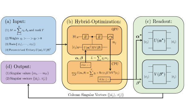
The input of our VQSVD algorithm is a decomposition of the matrix into a linear combination of unitaries of the form with real numbers . For instance, one could decompose into a linear combination of Pauli terms. And a method for finding such a decomposition was proposed in a recent work [51]. Several important generic matrices in engineering and science also exhibit LCUs, including Toeplitz, circulant, and Hankle matrices [52]. After taking in the inputs, our VQSVD algorithm enters a hybrid quantum-classical optimization loop to train the parameters and in the parameterized quantum circuits and via a designed loss (cf. Section 2.2). This loss function can be computed on quantum computers via the Hadamard tests. We then feeds the value of the loss function or its gradients (in gradient-based optimization) to a classical computer, which adjusts the parameters and for the next round of the loop. The goal is to find the global minimum of , i.e., .
In practice, one will need to set some termination condition (e.g., convergence tolerance) on the optimization loop. After the hybrid optimization, one will obtain values and optimal parameters and . The outputs approximate the singular values of , and approximate singular vectors of are obtained by inputting optimal parameters and into the parameterized circuits and in VQSVD and then applying to the orthonormal vectors for all . The detailed VQSVD algorithm is included in Algorithm 1. A schematic diagram is shown in Fig. 1.
2.2 Loss function
In this section, we provide more details and intuitions of the loss function in VQSVD. The key idea is to exploit the variational principles in matrix computation, which have great importance in analysis for error bounds of matrix analysis. In particular, the singular values satisfy a subtler variational property that incorporates both left and right singular vectors at the same time. For a given matrix , the largest singular value of can be characterized by
| (1) |
where is the set of pure states (normalized vectors) and Re means taking the real part. Moreover, by denoting the optimal singular vectors as , the remaining singular values () can be deduced using similar methods by restricting the unit vectors to be orthogonal to previous singular value vectors.
For a given matrix , the largest singular value of can be characterized by
| (2) |
where is the set of pure states (normalized vectors) and means to take the real part. Moreover, by denoting the optimal singular vectors as , the remaining singular values () can be deduced as follows
| (3) |
For a given matrix , the loss function in our VQSVD algorithm is defined as
| (5) |
where are real weights and is a set of orthonormal states. The setting of constants not only theoretically guarantees the correct outcome but also allows our approach to be more flexible. Usually, choosing these constants with excellent performances are empirical.
Theorem 1
For a given matrix , the loss function is maximized if only if
| (6) |
where are the largest singular values of and are orthonormal vectors. Moreover, and are left and right singular vectors, respectively.
Proof.
Let assume that are real numbers for simplicity, which could be achieved after the ideal maximization process.
Then we have
| (7) | ||||
| (8) | ||||
| (9) | ||||
| (10) |
Assume . The first inequality Eq. (8) follows due to the rearrangement inequality. The second inequality Eq. (10) follows due to property of singular values in Eq. (4). Note that the upper bound in Eq. (10) could be achieved if and only if for all , which is equivalent to
| (11) |
Therefore, the loss function is maximized if and only if extracts the singular values for each from to . Further, due to the variational property of singular values in Eq. (2) and Eq. (3), we conclude that the quantum neural networks and learn the singular vectors in the sense that and extract the left and right singular vectors, respectively.
In particular, the weights can be any sequence that satisfies the condition in Theorem 1. They are the key to train the quantum neural networks to learn the right singular vectors. Such weights can be understood as the tool to discriminate and identify the eigen-space.
Proposition 2
The loss function can be estimated on near-term quantum devices.
For with unitaries and real numbers , the quantity can be decomposed to
| (12) |
To estimate the quantity in Eq. (12), we could use quantum subroutines for estimating the quantity for a general unitary . One of these subroutines is to utilize the well-known Hadamard test [55], which requires only one ancillary qubit, one copy of state , and one controlled unitary operation , and hence it can be experimentally implemented on near term quantum hardware. To be specific, Hadamard test (see Fig. 2) starts with state , where denotes the ancillary qubit, and denotes the work register, and then apply a controlled unitary , conditioned on the qubit in register , to prepare state , at last, apply a Hadamard gate on the ancillary qubit, and measure. If the measurement outcome is , then let the output be ; otherwise, let the output be , and the expectation of output is . As for the imaginary part , it also can be estimated via Hadamard test by starting with state .
Remark 1: Notice that terms in Eq. (12) may be exponentially many for matrices with particular real-world applications, endowing a potential obstacle to the loss evaluation. However, we could apply the importance sampling technique to circumvent this issue. We provide a detailed discussion in Appendix B. In particular, we show that the loss evaluation efficiency is dependent on the -norm of all coefficients rather than the integer . Hence, for a matrix with a reasonable -norm (e.g., polynomial size), the evaluation could be efficient even for large-size problems. Besides, we take the circulant matrix as an example in Appendix B for illustration, suggesting the potential application of our approach in related practical fields.
2.3 As a generalization of the VQE family
In this subsection, we discuss the connection between our VQSVD algorithm and the variational quantum eigensolver (VQE) [25], which estimates the ground-state energy given a molecular electronic-structure Hamiltonian . This is a central problem to quantum chemistry as many properties of the molecule can be calculated once we determine the eigenstates of . Several related algorithms have been proposed to improve the spectrum learning capability of VQE (i.e., SSVQE [31]) such that the properties of excited states can also be explored. We consider these algorithms as a unified family and promising applications for quantum chemistry.
For practical reasons, one has to discretize the aforementioned Hamiltonian into a series of Pauli tensor products to work on quantum devices. Many physical models naturally fit into this scheme including the quantum Ising model and the Heisenberg Model. In particular, if the input of VQSVD in Eq. (5) is a Hamiltonian in a discretized form (i.e., a linear combination of Pauli tensor products or equivalently a Hermitian matrix), VQSVD could be naturally applied to diagonalize this Hamiltonian and prepare the eigenstates. Therefore, VQSVD can be seen as a generalization of the VQE family that works not only for Hamiltonians, but also for more general non-Hermitian matrices.
3 Optimization of the loss function
Finding optimal parameters is a significant part of variational hybrid quantum-classical algorithms. Both gradient-based and gradient-free methods could be used to do the optimization. Here, we provide analytical details on the gradient-based approach, and we refer to [56] for more information on the optimization subroutines in variational quantum algorithms. Reference about gradients estimation via quantum devices can be found in Ref. [57, 58, 30].
3.1 Gradients estimation
Here, we discuss the computation of the gradient of the global loss function by giving an analytical expression, and show that the gradients can be estimated by shifting parameters of the circuit used for evaluating the loss function. In Algorithm 1, to prepare states and , we apply gate sequences and in turn to state , where each gate and are either fixed, e.g., C-NOT gate, or parameterized, for all and . The parameterized gates and have forms and , respectively, where and are real parameters, and and are tensor products of Pauli matrices. Hence the gradient of loss function is dependent on parameters and the following proposition shows it can be computed on near-term quantum devices.
Proposition 3
The gradient of loss function can be estimated on near-term quantum devices and its explicitly form is defined as follows,
| (13) |
Particularly, the derivatives of with respect to and can be computed using following formulas, respectively,
| (14) | ||||
| (15) |
where notations and denote parameters and .
Proof.
Notice that the partial derivatives of loss function are given by Eqs. (14) (15), and hence the gradient is computed by shifting the parameters of circuits that are used to evaluate the loss function. Since the loss function can be estimated on near term quantum devices, claimed in Proposition 2, thus, the gradient can be calculated on near-term quantum devices.
3.2 Barren plateaus
It has been shown that when employing hardware-efficient ansatzes (usually problem agnostic) [59], global cost functions of an observable are untrainable for large problem sizes since they exhibit exponentially vanishing gradients with respect to the qubit number which makes the optimization landscape flat (i.e., barren plateaus [60]). Consequently, traditional optimization methods including the Adam optimizer utilized in our numerical experiments are impacted. This trainability issue happens even when the ansatz is short depth [61] and the work [62] showed that the barren plateau phenomenon could also arise in the architecture of dissipative quantum neural networks [63, 64, 65].
Several approaches have been proposed to mitigate this problem. One can either implementing identity-block initialization strategy [66] or employing the technique of local cost [61], where the local cost function is defined such that one firstly construct a local observable , calculating the expectation value with respect to each individual qubit rather than gathering information in a global sense, and finally adding up all the local contributions. The latter strategy has been verified to extend the trainable circuit depth up to . Recently, a new method of constructing adaptive Hamiltonians during the optimization loop has been proposed to resolve similar issues [67].
4 Numerical experiments and applications
Here we numerically simulate the VQSVD algorithm with randomly generated non-Hermitian real matrices as a proof of concept. Then, to demonstrate the possibility of scaling VQSVD to larger and more exciting applications, we simulate VQSVD to compress some standard gray-scale images. Fig. 3 shows the variational ansatz used. Since only real matrices are involved, the combination of rotation gates and CNOT is sufficient. For the case of complex matrices and different ansatzs, see Appendix C. We choose the input states to be and the circuit depth is set to be . The parameters are initialized randomly from an uniform distribution . All simulations and optimization loop are implemented via Paddle Quantum [68] on the PaddlePaddle Deep Learning Platform [69, 70].
4.1 Three-Qubit example
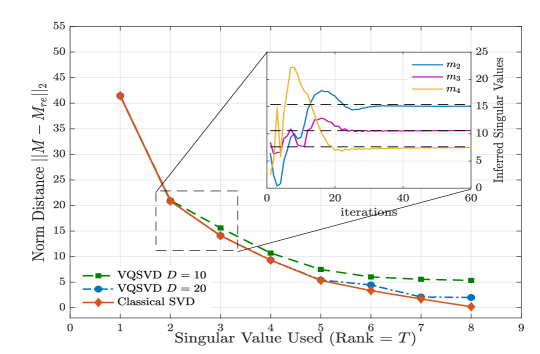
The VQSVD algorithm described in Section 2.1 can find largest singular values of matrix at once. Here, we choose the weight to be positive integers . Fig. 4 shows the learning process. One can see that this approach successfully find the desired singular values and one can approximate the original matrix with inferred singular values and vectors . The distance between and the original matrix is taken to be the matrix norm where are the matrix elements. As illustrated in Fig. 4, the distance decreases as more and more singular values being used.
4.2 Image compression
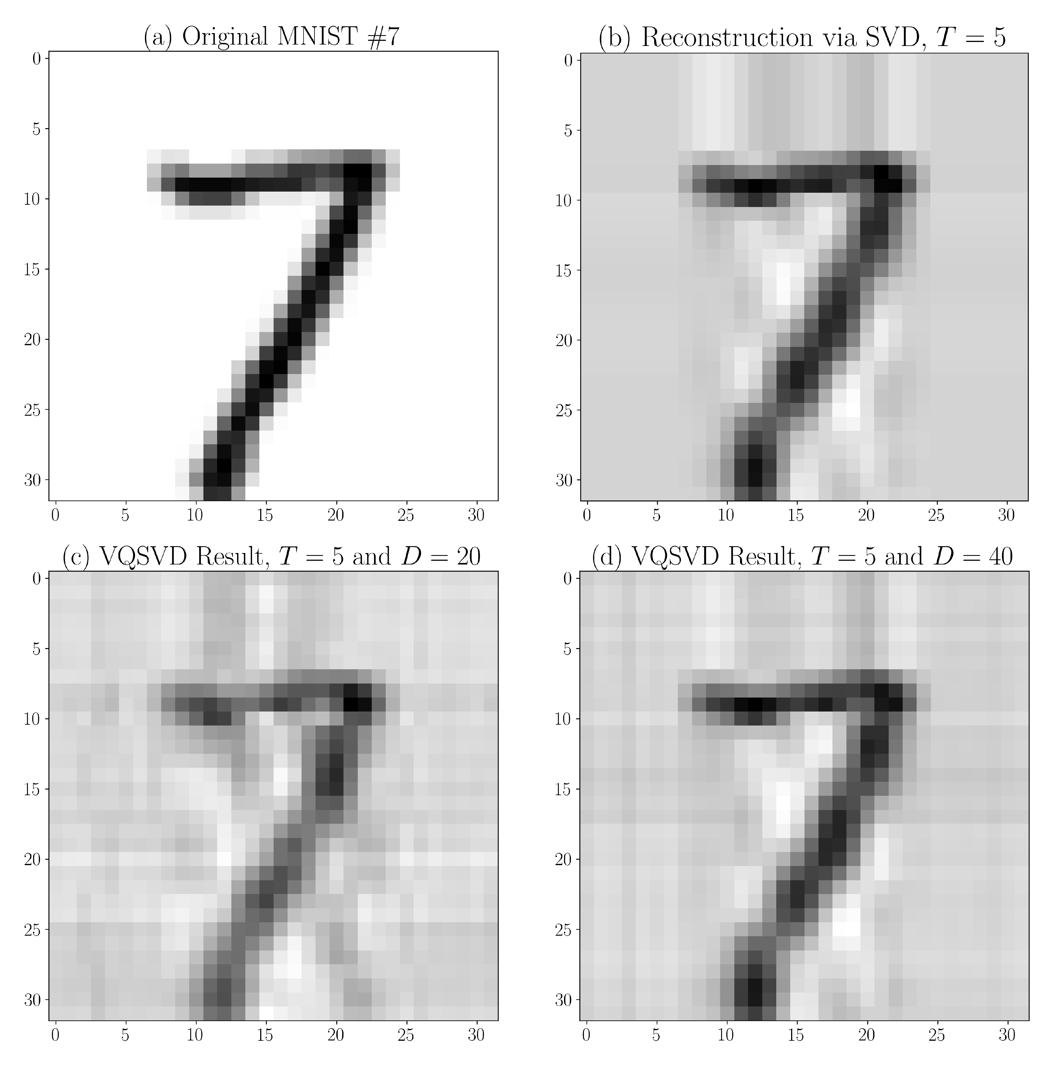
Next, we apply the VQSVD algorithm to compress a pixel handwritten digit image taken from the MNIST dataset with only (choose rank to be ) of its original information. By comparing with the classical SVD method, one can see that the digit is successfully reconstructed with some background noise. Notice the circuit structure demonstrated in Fig. 3 is ordinary and it is a not well-studied topic for circuit architecture. Future studies are needed to efficiently load classical information into NISQ devices beyond the LCU assumption.
5 Solution quality estimation
After obtaining the results (singular values and vectors) from Algorithm 1, it is natural and desirable to have a method to benchmark or verify these results. In this section, we further introduce a procedure for verification purposes. Particularly, we propose a variational quantum algorithm for estimating the sum of largest squared singular values, i.e., , of a matrix as a subroutine. In the following, we first define the error of the inferred singular values and singular vectors, and then show its estimation via a tool provided in Algorithm 3.
Let denote the inferred singular values of the matrix that are arranged in descending order, and let () denote the associated inferred left (right) singular vectors. The error of inferred singular values is defined as follows,
| (16) |
where s are the exact singular values of matrix and also arranged in descending order. And the error of inferred singular vectors is defined below,
| (17) |
where is a Hermitian operator of the form , and . It is worth pointing out that when inferred vectors approximate the eigenvectors of , i.e., , inferred singular vectors and approximate the singular vectors and respectively, and vice versa.
6 Applications
In this section, we give a brief discussion about the application of VQSVD in recommendation systems, and some other problems such as polar decomposition.
Recommendation systems
The goal of a recommendation system is to provide personalized items to customers based on their ratings of items, or other information. Usually, the preferences of customers are modeled by an matrix , where we assume there are customers and items. The element indicates the level that customer rates the item . In particular, finding suitable recommendations means to locate the large entries of rows.
One commonly used method for locating the large entries of rows is matrix reconstruction. Given an arbitrary matrix and integer , the goal is to output a small -rank matrix as an approximate matrix. In recommendation system, such an low-rank approximate matrix of the preference matrix is usually used to recommend items. In this sense, our VQSVD algorithm finds its application in recommendation system by learning such a small rank matrix. To be more specific, the information about its singular values and vectors can be obtained.
After obtaining the low rank matrix , the process of recommendation for customer proceeds as follows: project the th row vector of onto the space spanned by the right singular vectors of . Specifically, denote the right singular vectors of by , and projection operator by , then apply to the th normalized row vectors of . Specially, let denote the normalized vector after projection, given below:
| (20) |
where the right singular vectors form an orthogonal basis, are the corresponding coefficients, and denotes the normalization factor, i.e., .
The state can be efficiently prepared via paramerized circuit as long as we can prepare the state . Particularly, there are coefficients in Eq. (20), determining . Further, we present a procedure for estimating these coefficients in Algorithm 2 (shown below).
Finally, measure in the computational basis and output the outcome.
Polar decomposition and other applications
Another important application of our VQSVD algorithm is finding the polar decomposition which has many applications in linear algebra [71, 72]. Recently, Lloyd et al [73] proposed a quantum polar decomposition algorithm that performs in a deterministic way. For a given a complex matrix , the right polar decomposition is defined as follows,
| (21) |
where is a unitary and is a positive-semidefinite Hermitian matrix. Particularly, suppose the singular value decomposition of is calculated through the VQSVD algorithm , then and . It is interesting to explore whether our VQSVD could be applied to polar decomposition.
For Hermitian matrices, the VQSVD algorithm can be applied as an eigensolver since singular value decomposition reduces to spectral decomposition in this case. Recently, some work has been proposed to extract eigenvalues and reconstruct eigenvectors of Hermitian matrices [74, 31], density operators [75].
In the context of quantum information, SVD could be used to compute the Schmidt decomposition of bipartite pure states and we note that our VQSVD algorithm could also be applied to do Schmidt decomposition. Meanwhile, a recent work by Bravo-Prieto et al. [76] introduces a novel varitional quantum algorithm for obtaining the Schmidt coefficients and associated orthonormal vectors of a bipartite pure state. In comparison, our VQSVD algorithm can deal with the SVD of the general matrix, while Ref. [76] is intended for the Schmidt decomposition of bipartite pure states.
7 Discussion and outlook
To summarize, we have presented a variational quantum algorithm for singular value decomposition with NISQ devices. One key contribution is to design a loss function that could be used to train the quantum neural networks to learn the left and right singular vectors and output the target singular values. Further improvements on the performance of our VQSVD algorithm may be done for sparse matrices together with more sophisticated ansatzes. We have numerically verified our algorithm for singular value decomposition of random matrices and image compression and proposed extensive applications in solving linear systems of equations. As a generalization of the family of VQE algorithms on Hamiltonian diagonalization (or spectral decomposition), the VQSVD algorithm may have potential applications in quantum chemistry, quantum machine learning. and quantum optimization in the NISQ era.
Our algorithm theoretically works well for large-scale problems if we could have carefully handled the trainability and accuracy of QNN. Just like regular variational quantum algorithms, there are still several challenges that need to be addressed to maintain the hope of achieving quantum speedups when scaling up to large-scale problems on NISQ devices. We refer to the recent review papers [22, 23, 24] for potential solutions to these challenges.
One future direction is to develop near-term quantum algorithms for non-negative matrix factorization [3] which have various applications and broad interests in machine learning. See [77] as an example of the quantum solution. Another interesting direction is to develop near-term quantum algorithms for higher-order singular value decomposition [78].
Acknowledgements
We would like to thank Runyao Duan for helpful discussions. This work was done when Z. S. was a research intern at Baidu Research. Y. W. acknowledged support from the Baidu-UTS AI Meets Quantum project and the Australian Research Council (Grant No: DP180100691).
References
- Boyd and Vandenberghe [2004] Stephen Boyd and Lieven Vandenberghe. Convex optimization. Cambridge university press, 2004. ISBN 1107394007. doi: 10.1017/CBO9780511804441.
- Murphy [2012] Kevin P Murphy. Machine learning: a probabilistic perspective. MIT press, 2012. ISBN 0262304325. URL https://amstat.tandfonline.com/doi/abs/10.1080/09332480.2014.914768.
- Koren et al. [2009] Yehuda Koren, Robert Bell, and Chris Volinsky. Matrix factorization techniques for recommender systems. Computer, 42(8):30–37, 2009. ISSN 0018-9162. doi: 10.1109/MC.2009.263.
- Shor [1997] Peter W. Shor. Polynomial-Time Algorithms for Prime Factorization and Discrete Logarithms on a Quantum Computer. SIAM Journal on Computing, 26(5):1484–1509, Oct 1997. ISSN 0097-5397. doi: 10.1137/S0097539795293172.
- Grover [1996] Lov K Grover. A fast quantum mechanical algorithm for database search. In Proceedings of the twenty-eighth annual ACM symposium on Theory of computing - STOC ’96, pages 212–219, New York, New York, USA, 1996. ACM Press. ISBN 0897917855. doi: 10.1145/237814.237866.
- Harrow et al. [2009] Aram W Harrow, Avinatan Hassidim, and Seth Lloyd. Quantum Algorithm for Linear Systems of Equations. Physical Review Letters, 103(15):150502, Oct 2009. doi: 10.1103/PhysRevLett.103.150502.
- Clader et al. [2013] B David Clader, Bryan C Jacobs, and Chad R Sprouse. Preconditioned Quantum Linear System Algorithm. Physical Review Letters, 110(25):250504, jun 2013. ISSN 0031-9007. doi: 10.1103/PhysRevLett.110.250504.
- Childs et al. [2017] Andrew M. Childs, Robin Kothari, and Rolando D. Somma. Quantum Algorithm for Systems of Linear Equations with Exponentially Improved Dependence on Precision. SIAM Journal on Computing, 46(6):1920–1950, Jan 2017. ISSN 0097-5397. doi: 10.1137/16M1087072.
- Wossnig et al. [2018] Leonard Wossnig, Zhikuan Zhao, and Anupam Prakash. Quantum Linear System Algorithm for Dense Matrices. Physical Review Letters, 120(5):050502, Jan 2018. ISSN 0031-9007. doi: 10.1103/PhysRevLett.120.050502.
- Subasi et al. [2018] Yigit Subasi, Rolando D. Somma, and Davide Orsucci. Quantum algorithms for systems of linear equations inspired by adiabatic quantum computing. Physical Review Letters, 122(6):060504, May 2018. ISSN 0031-9007. doi: 10.1103/PhysRevLett.122.060504.
- Brandao and Svore [2017] Fernando G.S.L. Brandao and Krysta M. Svore. Quantum Speed-Ups for Solving Semidefinite Programs. In 2017 IEEE 58th Annual Symposium on Foundations of Computer Science (FOCS), pages 415–426. IEEE, Oct 2017. ISBN 978-1-5386-3464-6. doi: 10.1109/FOCS.2017.45.
- Chakrabarti et al. [2020] Shouvanik Chakrabarti, Andrew M Childs, Tongyang Li, and Xiaodi Wu. Quantum algorithms and lower bounds for convex optimization. Quantum, 4:221, Jan 2020. ISSN 2521-327X. doi: 10.22331/q-2020-01-13-221.
- Brandão et al. [2019] Fernando G S L Brandão, Amir Kalev, Tongyang Li, Cedric Yen-Yu Lin, Krysta M Svore, and Xiaodi Wu. Quantum SDP Solvers: Large Speed-Ups, Optimality, and Applications to Quantum Learning, ICALP 2019, doi: 10.4230/LIPIcs.ICALP.2019.27
- van Apeldoorn et al. [2020] Joran van Apeldoorn, András Gilyén, Sander Gribling, and Ronald de Wolf. Convex optimization using quantum oracles. Quantum, 4:220, Jan 2020. ISSN 2521-327X. doi: 10.22331/q-2020-01-13-220.
- Biamonte et al. [2017] Jacob Biamonte, Peter Wittek, Nicola Pancotti, Patrick Rebentrost, Nathan Wiebe, and Seth Lloyd. Quantum machine learning. Nature, 549(7671):195–202, Sep 2017. ISSN 0028-0836. doi: 10.1038/nature23474.
- Schuld and Petruccione [2018] Maria Schuld and Francesco Petruccione. Supervised Learning with Quantum Computers. Quantum Science and Technology. Springer International Publishing, 2018. ISBN 978-3-319-96423-2. doi: 10.1007/978-3-319-96424-9.
- Ciliberto et al. [2018] Carlo Ciliberto, Mark Herbster, Alessandro Davide Ialongo, Massimiliano Pontil, Andrea Rocchetto, Simone Severini, and Leonard Wossnig. Quantum machine learning: a classical perspective. Proceedings of the Royal Society A: Mathematical, Physical and Engineering Sciences, 474(2209):20170551, Jan 2018. ISSN 1364-5021. doi: 10.1098/rspa.2017.0551.
- Kerenidis and Prakash [2016] Iordanis Kerenidis and Anupam Prakash. Quantum Recommendation Systems. arXiv preprint arXiv:1603.08675, pages 1–22, Mar 2016. URL http://arxiv.org/abs/1603.08675.
- Rebentrost et al. [2018] Patrick Rebentrost, Adrian Steffens, Iman Marvian, and Seth Lloyd. Quantum singular-value decomposition of nonsparse low-rank matrices. Physical Review A, 97(1):012327, Jan 2018. ISSN 2469-9926. doi: 10.1103/PhysRevA.97.012327.
- Preskill [2018] John Preskill. Quantum Computing in the NISQ era and beyond. Quantum, 2:79, Aug 2018. ISSN 2521-327X. doi: 10.22331/q-2018-08-06-79.
- McClean et al. [2016] Jarrod R. McClean, Jonathan Romero, Ryan Babbush, and Alán Aspuru-Guzik. The theory of variational hybrid quantum-classical algorithms. New Journal of Physics, 18(2):023023, Feb 2016. ISSN 1367-2630. doi: 10.1088/1367-2630/18/2/023023.
- Cerezo et al. [2020a] M. Cerezo, Andrew Arrasmith, Ryan Babbush, Simon C. Benjamin, Suguru Endo, Keisuke Fujii, Jarrod R. McClean, Kosuke Mitarai, Xiao Yuan, Lukasz Cincio, and Patrick J. Coles. Variational Quantum Algorithms. arXiv:2012.09265, pages 1–29, Dec 2020a. URL http://arxiv.org/abs/2012.09265.
- Endo et al. [2020] Suguru Endo, Zhenyu Cai, Simon C Benjamin, and Xiao Yuan. Hybrid quantum-classical algorithms and quantum error mitigation. arXiv:2011.01382, pages 1–39, Nov 2020. URL http://arxiv.org/abs/2011.01382.
- Bharti et al. [2021] Kishor Bharti, Alba Cervera-Lierta, Thi Ha Kyaw, Tobias Haug, Sumner Alperin-Lea, Abhinav Anand, Matthias Degroote, Hermanni Heimonen, Jakob S Kottmann, Tim Menke, Wai-Keong Mok, Sukin Sim, Leong-Chuan Kwek, and Alán Aspuru-Guzik. Noisy intermediate-scale quantum (NISQ) algorithms. arXiv:2101.08448, pages 1–82, Jan 2021. URL http://arxiv.org/abs/2101.08448.
- Peruzzo et al. [2014] Alberto Peruzzo, Jarrod McClean, Peter Shadbolt, Man-Hong Yung, Xiao-Qi Zhou, Peter J Love, Alán Aspuru-Guzik, and Jeremy L O’Brien. A variational eigenvalue solver on a photonic quantum processor. Nature Communications, 5(1):4213, Sep 2014. ISSN 2041-1723. doi: 10.1038/ncomms5213.
- McClean et al. [2017] Jarrod R. McClean, Mollie E. Kimchi-Schwartz, Jonathan Carter, and Wibe A. de Jong. Hybrid quantum-classical hierarchy for mitigation of decoherence and determination of excited states. Physical Review A, 95(4):042308, Apr 2017. ISSN 2469-9926. doi: 10.1103/PhysRevA.95.042308.
- Higgott et al. [2019] Oscar Higgott, Daochen Wang, and Stephen Brierley. Variational Quantum Computation of Excited States. Quantum, 3:156, Jul 2019. ISSN 2521-327X. doi: 10.22331/q-2019-07-01-156.
- Barkoutsos et al. [2020] Panagiotis Kl Barkoutsos, Giacomo Nannicini, Anton Robert, Ivano Tavernelli, and Stefan Woerner. Improving Variational Quantum Optimization using CVaR. Quantum, 4(Section II):256, Apr 2020. ISSN 2521-327X. doi: 10.22331/q-2020-04-20-256.
- Nakanishi et al. [2019a] Ken M Nakanishi, Kosuke Mitarai, and Keisuke Fujii. Subspace-search variational quantum eigensolver for excited states. Physical Review Research, 1(3):033062, Oct 2019a. ISSN 2643-1564. doi: 10.1103/PhysRevResearch.1.033062.
- Ostaszewski et al. [2019] Mateusz Ostaszewski, Edward Grant, and Marcello Benedetti. Quantum circuit structure learning. arXiv:1905.09692, pages 1–11, May 2019. URL http://arxiv.org/abs/1905.09692.
- Nakanishi et al. [2019b] Ken M Nakanishi, Kosuke Mitarai, and Keisuke Fujii. Subspace-search variational quantum eigensolver for excited states. Physical Review Research, 1(3):033062, 2019b. doi: 10.1103/PhysRevResearch.1.033062.
- Cerezo et al. [2019] M Cerezo, Alexander Poremba, Lukasz Cincio, and Patrick J Coles. Variational Quantum Fidelity Estimation. Quantum 4, 248, 2020. doi: 10.22331/q-2020-03-26-248.
- [33] Ranyiliu Chen, Zhixin Song, Xuanqiang Zhao, and Xin Wang. Variational Quantum Algorithms for Trace Distance and Fidelity Estimation. arXiv:2012.05768, 2020. URL http://arxiv.org/abs/2012.05768.
- Wu and Hsieh [2019] Jingxiang Wu and Timothy H. Hsieh. Variational Thermal Quantum Simulation via Thermofield Double States. Physical Review Letters, 123(22):220502, 2019. ISSN 0031-9007. doi: 10.1103/PhysRevLett.123.220502.
- Chowdhury et al. [2020] Anirban N. Chowdhury, Guang Hao Low, and Nathan Wiebe. A Variational Quantum Algorithm for Preparing Quantum Gibbs States. pages 1–13, 2020. URL http://arxiv.org/abs/2002.00055.
- Wang et al. [2020] Youle Wang, Guangxi Li, and Xin Wang. Variational quantum Gibbs state preparation with a truncated Taylor series. arXiv:2005.08797, May 2020. URL http://arxiv.org/abs/2005.08797.
- Khatri et al. [2019] Sumeet Khatri, Ryan LaRose, Alexander Poremba, Lukasz Cincio, Andrew T. Sornborger, and Patrick J. Coles. Quantum-assisted quantum compiling. Quantum, 3:140, 2019. ISSN 2521-327X. doi: 10.22331/q-2019-05-13-140.
- Heya et al. [2018] Kentaro Heya, Yasunari Suzuki, Yasunobu Nakamura, and Keisuke Fujii. Variational Quantum Gate Optimization. 2018. URL http://arxiv.org/abs/1810.12745.
- Jones and Benjamin [2018] Tyson Jones and Simon C Benjamin. Quantum compilation and circuit optimisation via energy dissipation. pages 1–17, 2018. URL http://arxiv.org/abs/1811.03147.
- Sharma et al. [2020a] Kunal Sharma, Sumeet Khatri, M Cerezo, and Patrick J Coles. Noise resilience of variational quantum compiling. New Journal of Physics, 22(4):043006, 2020a. ISSN 1367-2630. doi: 10.1088/1367-2630/ab784c.
- [41] Chenfeng Cao and Xin Wang. Noise-Assisted Quantum Autoencoder. Physical Review Applied, 15(5):054012, 2021. doi: 10.1103/PhysRevApplied.15.054012.
- [42] Iris Cong, Soonwon Choi, Mikhail D. Lukin. Quantum convolutional neural networks. Nature Physics, 15(12):1273-1278, 2019. doi: 10.1038/s41567-019-0648-8.
- [43] Guangxi Li, Zhixin Song, and Xin Wang. VSQL: Variational shadow quantum learning for classification. Proceedings of the AAAI Conference on Artificial Intelligence, 35(9), 8357-8365, 2021. URL https://ojs.aaai.org/index.php/AAAI/article/view/17016.
- Temme et al. [2017] Kristan Temme, Sergey Bravyi, and Jay M. Gambetta. Error Mitigation for Short-Depth Quantum Circuits. Physical Review Letters, 119(18):180509, 2017. doi: 10.1103/PhysRevLett.119.180509.
- McArdle et al. [2019] Sam McArdle, Xiao Yuan, and Simon Benjamin. Error-Mitigated Digital Quantum Simulation. Physical Review Letters, 122(18):180501, 2019. ISSN 0031-9007. doi: 10.1103/PhysRevLett.122.180501.
- Strikis et al. [2020] Armands Strikis, Dayue Qin, Yanzhu Chen, Simon C Benjamin, and Ying Li. Learning-based quantum error mitigation. arXiv:2005.07601, pages 1–19, 2020. URL http://arxiv.org/abs/2005.07601.
- Kandala et al. [2019] Abhinav Kandala, Kristan Temme, Antonio D. Córcoles, Antonio Mezzacapo, Jerry M. Chow, and Jay M. Gambetta. Error mitigation extends the computational reach of a noisy quantum processor. Nature, 567(7749):491–495, 2019. ISSN 0028-0836. doi: 10.1038/s41586-019-1040-7.
- [48] Jiaqing Jiang, Kun Wang, and Xin Wang. Physical Implementability of Quantum Maps and Its Application in Error Mitigation. arXiv:2012.10959, 2020. URL http://arxiv.org/abs/2012.10959.
- [49] Kun Wang, Yu-Ao Chen, and Xin Wang. Measurement Error Mitigation via Truncated Neumann Series. arXiv:2103.13856, 2021. URL http://arxiv.org/abs/2103.13856.
- Larose et al. [2019] Ryan Larose, Arkin Tikku, Étude O Neel-judy, Lukasz Cincio, and Patrick J Coles. Variational quantum state diagonalization. npj Quantum Information, (November 2018), 2019. ISSN 2056-6387. doi: 10.1038/s41534-019-0167-6.
- Gunlycke et al. [2020] Daniel Gunlycke, Mark C. Palenik, Alex R. Emmert, and Sean A. Fischer. Efficient algorithm for generating Pauli coordinates for an arbitrary linear operator. arXiv:2011.08942, 2020. URL http://arxiv.org/abs/2011.08942.
- Wan et al. [2019] Lin-Chun Wan, Chao-Hua Yu, Shi-Jie Pan, Yi-Jie Shi, Su-Juan Qin, Fei Gao, and Qiao-Yan Wen. Implementing block-encoding with a decomposition of linear combination of unitaries. arXiv:1912.12212, 2019. URL https://arxiv.org/pdf/1912.12212.
- Fan [1951] Ky Fan. Maximum properties and inequalities for the eigenvalues of completely continuous operators. Proceedings of the National Academy of Sciences of the United States of America, 37(11):760, 1951. URL https://www.jstor.org/stable/88481?seq=1#metadata_info_tab_contents.
- Zhang [2015] Zhihua Zhang. The Singular Value Decomposition, Applications and Beyond. arXiv:1510.08532, 2015. URL http://arxiv.org/abs/1510.08532.
- Aharonov et al. [2009] Dorit Aharonov, Vaughan Jones, and Zeph Landau. A Polynomial Quantum Algorithm for Approximating the Jones Polynomial. Algorithmica, 55(3):395–421, 2009. ISSN 0178-4617. doi: 10.1007/s00453-008-9168-0.
- Benedetti et al. [2019] Marcello Benedetti, Erika Lloyd, Stefan Sack, and Mattia Fiorentini. Parameterized quantum circuits as machine learning models. Quantum Science and Technology, 4(4):043001, 2019. ISSN 2058-9565. doi: 10.1088/2058-9565/ab4eb5.
- Mitarai et al. [2018] K. Mitarai, M. Negoro, M. Kitagawa, and K. Fujii. Quantum circuit learning. Physical Review A, 98(3):032309, 2018. ISSN 2469-9926. doi: 10.1103/PhysRevA.98.032309.
- Schuld et al. [2019] Maria Schuld, Ville Bergholm, Christian Gogolin, Josh Izaac, and Nathan Killoran. Evaluating analytic gradients on quantum hardware. Physical Review A, 99(3):032331, 2019. ISSN 24699934. doi: 10.1103/PhysRevA.99.032331.
- Kandala et al. [2017] Abhinav Kandala, Antonio Mezzacapo, Kristan Temme, Maika Takita, Markus Brink, Jerry M. Chow, and Jay M. Gambetta. Hardware-efficient variational quantum eigensolver for small molecules and quantum magnets. Nature, 549(7671):242–246, sep 2017. ISSN 0028-0836. doi: 10.1038/nature23879.
- McClean et al. [2018] Jarrod R. McClean, Sergio Boixo, Vadim N. Smelyanskiy, Ryan Babbush, and Hartmut Neven. Barren plateaus in quantum neural network training landscapes. Nature Communications, 9(1):4812, 2018. ISSN 2041-1723. doi: 10.1038/s41467-018-07090-4.
- Cerezo et al. [2020b] M Cerezo, Akira Sone, Tyler Volkoff, Lukasz Cincio, and Patrick J Coles. Cost-Function-Dependent Barren Plateaus in Shallow Quantum Neural Networks. Nature Communications 12:1791, 2021b. doi: 10.1038/s41467-021-21728-w
- Sharma et al. [2020b] Kunal Sharma, M Cerezo, Lukasz Cincio, and Patrick J Coles. Trainability of Dissipative Perceptron-Based Quantum Neural Networks. arXiv:2005.12458, 2020b.
- Poland et al. [2020] Kyle Poland, Kerstin Beer, and Tobias J. Osborne. No Free Lunch for Quantum Machine Learning. arXiv:2003.14103, 2020. URL http://arxiv.org/abs/2003.14103.
- Bondarenko and Feldmann [2020] Dmytro Bondarenko and Polina Feldmann. Quantum Autoencoders to Denoise Quantum Data. Physical Review Letters, 124(13):130502, mar 2020. ISSN 0031-9007. doi: 10.1103/PhysRevLett.124.130502.
- Beer et al. [2020] Kerstin Beer, Dmytro Bondarenko, Terry Farrelly, Tobias J. Osborne, Robert Salzmann, Daniel Scheiermann, and Ramona Wolf. Training deep quantum neural networks. Nature Communications, 11(1):808, dec 2020. ISSN 2041-1723. doi: 10.1038/s41467-020-14454-2.
- Grant et al. [2019] Edward Grant, Leonard Wossnig, Mateusz Ostaszewski, and Marcello Benedetti. An initialization strategy for addressing barren plateaus in parametrized quantum circuits. Quantum, 3:214, 2019. doi: 10.22331/q-2019-12-09-214
- Cerezo et al. [2020c] M. Cerezo, Kunal Sharma, Andrew Arrasmith, and Patrick J. Coles. Variational Quantum State Eigensolver. arXiv:2004.01372, (1):1–14, 2020c. URL http://arxiv.org/abs/2004.01372.
- Pad [2020] Paddle Quantum: a quantum machine learning toolkit, 2020. URL https://qml.baidu.com.
- [69] PaddlePaddle URL https://github.com/paddlepaddle/paddle.
- Ma et al. [2019] Yanjun Ma, Dianhai Yu, Tian Wu, and Haifeng Wang. PaddlePaddle: An Open-Source Deep Learning Platform from Industrial Practice. Frontiers of Data and Domputing, 1(1):105–115, 2019. ISSN 1674-9480. doi: 10.11871/jfdc.issn.2096.742X.2019.01.011
- Higham [1986] Nicholas J Higham. Computing the polar decomposition—with applications. SIAM Journal on Scientific and Statistical Computing, 7(4):1160–1174, 1986. doi: 10.1137/0907079
- Gower et al. [2004] John C Gower, Garmt B Dijksterhuis, et al. Procrustes problems, volume 30. Oxford University Press on Demand, 2004. URL http://oro.open.ac.uk/2736/.
- Lloyd et al. [2020] Seth Lloyd, Samuel Bosch, Giacomo De Palma, Bobak Kiani, Zi-Wen Liu, Milad Marvian, Patrick Rebentrost, and David M Arvidsson-Shukur. Quantum polar decomposition algorithm. arXiv preprint arXiv:2006.00841, 2020. URL https://arxiv.org/abs/2006.00841.
- Jones et al. [2019] Tyson Jones, Suguru Endo, Sam McArdle, Xiao Yuan, and Simon C. Benjamin. Variational quantum algorithms for discovering Hamiltonian spectra. Physical Review A, 99(6):062304, jun 2019. ISSN 2469-9926. doi: 10.1103/PhysRevA.99.062304.
- LaRose et al. [2019] Ryan LaRose, Arkin Tikku, Étude O’Neel-Judy, Lukasz Cincio, and Patrick J Coles. Variational quantum state diagonalization. npj Quantum Information, 5(1):1–10, 2019. doi: 10.1038/s41534-019-0167-6
- Bravo-Prieto et al. [2019a] Carlos Bravo-Prieto, Diego Garcia-Martin, and Jose I. Latorre. Quantum Singular Value Decomposer. Physical Review A, 101, 062310, 2020a. doi: 10.1103/PhysRevA.101.062310
- Du et al. [2018] Yuxuan Du, Tongliang Liu, Yinan Li, Runyao Duan, and Dacheng Tao. Quantum divide-and-conquer anchoring for separable non-negative matrix factorization. In Proceedings of the 27th International Joint Conference on Artificial Intelligence, pages 2093–2099, 2018. doi: 10.5555/3304889.3304950
- Kolda and Bader [2009] Tamara G Kolda and Brett W Bader. Tensor decompositions and applications. SIAM review, 51(3):455–500, 2009. ISSN 0036-1445. doi: 10.1137/07070111X
- Bravo-Prieto et al. [2019b] Carlos Bravo-Prieto, Ryan LaRose, M. Cerezo, Yigit Subasi, Lukasz Cincio, and Patrick J. Coles. Variational Quantum Linear Solver: A Hybrid Algorithm for Linear Systems. arXiv:1909.05820, 2019b. URL http://arxiv.org/abs/1909.05820.
Appendix A Proof details for Proposition 3
In this section, we show a full derivation on the gradients of the loss function in our VQSVD algorithm.
| (22) |
The real part can be estimated via Hadamard test. Equivalently saying that,
| (23) |
Consider the parametrized quantum circuit and . For convenience, denote . We can write the cost function as:
| (24) |
Absorb most gates into state and matrix ,
| (25) |
where , and . We assume is generated by a Pauli product and same for . The derivative with respect to a certain angle is
| (26) | ||||
| (27) |
Thus the gradient is calculated to be
| (28) |
With the following property, we can absorb the Pauli product by an rotation on
| (29) |
Plug it back and we get,
| (30) |
This can be further simplified as
| (31) |
Similarly, for we have
| (32) |
This can be further simplified as
| (33) |
One can see from the above derivation that calculating the analytical gradient of VQSVD algorithm simply means rotating a specific gate parameter (angle or ) by which can be easily implemented on near-term quantum devices.
Appendix B Supplemental material for cost evaluation
In this section, we show how to apply the importance sampling technique to reduce the cost of estimating the loss function in Eq. (12). For convenience, we restate Eq. (12) below.
| (34) |
We assume all coefficients in Eq. (12) are positive, since their signs can be absorbed into unitaries .
Define an importance sampling in a sense that
| (35) |
where , and denotes the -norm. Random variable indicates that each unitary is selected at random with probability proportional to its weight. Here, we rewrite Eq. (34) by using .
| (36) |
As is formed as an expectation, the sample mean is supposed to estimate it. By Chebyshev’s inequality, samples suffice to compute an estimate up to precision with high probability, where denotes the variance, and denotes the precision. By Chernoff bound, the probability can be further improved to costing an additional multiplicative factor . Regarding , the variance is bounded by . We, therefore, only need to choose many unitaries to evaluate . Viewed from this point, the cost of the evaluation is dependent on the instead of the integer . As a result, the loss evaluation could be efficient if the is small, even there are exponentially many terms.
Example. Suppose we use VQSVD to compute SVDs of circulant matrices, which have applications in signal processing, image compression, number theory and cryptography. A circulant matrix is given by
| (37) |
Clearly, the matrix is determined by the sequence . It can be easily decomposed into a weighted sum of cyclic permutations.
| (38) |
where
The loss for a circulant matrix in Eq. (34) is given by
| (39) |
Hence, for circulant matrices with feasible cost (e.g., polynomial size), the loss evaluation could be quite efficient even for large-size problems. Our VQSVD algorithm is expected to find further applications in circulant matrix-related problems.
Appendix C Supplemental material for different ansatzs
In this section, we supplement additional numerics on real matrices to explore the effect of different circuit ansatzs and later test our VQSVD algorithm on random complex matrices. First, we introduce several ansatz candidates.
(a) \Qcircuit@C=0.7em @R=0.4em
&\gateU\ctrl1\qw\qw
\gateU\targ\ctrl1\qw
\gateU\qw\targ\qw^ ×D_1
\gategroup12342.07em–
(b) \Qcircuit@C=0.7em @R=0.4em
&\gateU\ctrl1\gateU \qw\qw\qw\qw
\gateU\targ\gateU \gateU\ctrl1\gateU\qw
\qw\qw\qw\gateU\targ\gateU\qw^ ×D_2
\gategroup12372.07em–
(c) \Qcircuit@C=0.7em @R=0.4em
&\gateU \ctrl1\qw\targ\qw
\gateU \targ\ctrl1\qw\qw
\gateU \qw\targ\ctrl-2 \qw^ ×D_3
\gategroup12352.07em–
(d) \Qcircuit@C=0.7em @R=0.4em
&\gateU \ctrl1\qw\gateU \targ\qw\qw
\gateU \targ\ctrl1 \gateU \qw\targ\qw
\gateU \qw\targ\gateU \ctrl-2 \ctrl-1\qw^ ×D_4
\gategroup12372.07em–
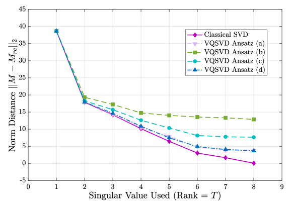
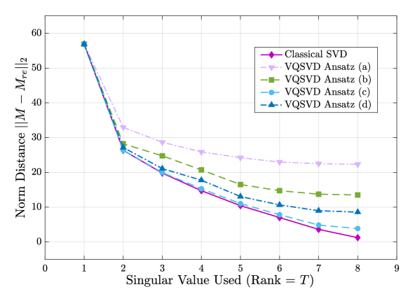
After introducing all the candidates, we test the distance measure on a real matrix similar to Fig. 4. For fair comparison, we want all the ansatz candidates to have the same total amount of trainable parameters and leads to the specific depth . Other setups including desired rank , the weight coefficient , the random seed for generating trainable parameters, number of optimization iterations ITR=200, learning rate LR=0.05, and the Adam optimizer are fixed. The result is illustrated in Fig. 7. The advantage of candidate (a) and (d) is observed consistently in numerical experiments. Finally, we repeat the same experiments on random complex matrices. No clear advantage of a specific ansatz candidate is observed under this setup. Most of the time, candidate (a), (c) and (d) would return a better result compare to candidate (b). But in certain cases, the performance of candidate (a) could be very bad due to the lack of entangling capability. We report a case study in Fig. 8. Further studies are needed to check more ansatz candidates by manipulating the entangling structure.
Appendix D Supplemental material for verification of the solution quality
In this section, we provide the necessary proofs in Sec. 5 and detailed discussions on variational quantum Frobenius norm estimation algorithm.
D.1 Definitions
Recall that the error of inferred singular values is defined as follows,
| (40) |
where are the exact singular values of matrix and also arranged in descending order. And the error of inferred singular vectors is defined below,
| (41) |
where is a Hermitian of the form , and . The quantity quantifies the component of that is perpendicular to , which follows from .
It is worth pointing out that when inferred vectors approximate the eigenvectors , where , of , i.e., , inferred singular vectors and approximate the singular vectors and respectively, and vice versa. On the other hand, the error which is used to quantify the extent that vectors approximate eigenvector can quantify the extent that inferred vectors and approximate the singular vectors. Specifically, these distances have an equal relation, which is depicted in the following equation.
| (42) |
where denotes the distance between vectors.
Here, we give the explicit forms of the distances . (42). The distances between and are defined in the following form,
| (43) | ||||
| (44) |
And the distances between and are defined below,
| (45) | ||||
| (46) |
Notice that both of the Right-Hand-Sides of Eqs. (44), (46) are equivalent to , and then the relation in Eq. (42) follows.
D.2 Error analysis
After running VQSVD, it would be ideal if we can verify the quality of the outputs from VQSVD. For achieving this purpose, we show that these error and are upper bounded and give the explicit form of upper bounds. We present the derivation for upper bounds on errors in the following lemma.
Lemma 4
Proof.
Recall the definitions of and in Eqs. (40), (41), and notice that
| (47) |
Since the dot product with decreasingly ordered coefficients is Schur-convex and majorize , i.e., for all , then , which results an upper bound on error .
Note that the error can be rewritten as
| (48) |
and eigenvectors can be expanded into a basis of the space, then we have
| (49) | ||||
| (50) |
D.3 A tool for solution quality estimation
The goal of this section is to provide a tool that computes the sum of largest squared singular values, which is used in Sec. 5 to analyze the accuracy of outputs of VQSVD. In the following, we mainly show the correctness analysis of Algorithm 3. The detailed discussions on loss evaluation and gradients estimation are omitted, since we can employ the same methods introduced in Ref. [79] to loss evaluation and gradients derivation. The differences of our method from that in Ref. [79] occur in input states. Specifically, we input computational states for all into the circuit, while they input state . For more information on loss evaluation and gradients derivation, we refer the interested readers to Ref. [79].
Correctness analysis
The validity of Algorithm 3 follows from a fact that, for arbitrary matrix, its squared singular values majorize the squared norms of diagonal elements. Specifically, the sum of the largest squared singular values is larger than the sum of squared norms of the largest diagonal elements. We summarize this fact in the lemma below and further provide a proof.
Lemma 5
For arbitrary matrix , let singular values of be , which are arranged in descending order. Then for any , we have the following inequality:
| (51) |
where is the diagonal vector of , i.e., , and the notation means that the are arranged in descending order. In particular, the equality holds if and only if is diagonal.
Proof.
The core of the proof is to connect singular values and diagonal elements. Specifically, this process can been done with the following inequalities:
| (52) | |||
| (53) |
where are singular values of , and is the vector denoting the diagonal elements of . The first inequality Eqs. (52) can be derived since eigenvalues of a Hermitian matrix majorize its diagonal elements. As s are the eigenvalues of , we have
| (54) |
for any . Second, note that diagonal elements of , i.e., , can be expressed in the following form:
| (55) |
Then, from Eq. (55), we can easily derive inequalities below:
| (56) |
where sum includes the largest absolute values of diagonal elements , and set contains indices of rows that all belong. Here we explain inequalities in Eq. (56). The second inequality holds since the sum contains entries of rows that locate. Thus it not only contains the diagonal elements that appear in the sum but also other off-diagonal elements. Meanwhile, recall that the sum consists of the largest diagonal elements of matrix . Thus it must be larger than any sum that contains some diagonal elements of , validating the first inequality.
Loss evaluation
We consider the evaluation of in VQFNE, which can be rewritten as
| (57) | ||||
| (58) |
In principle, these inner products in Eq. (58) can be efficiently estimated via Hadamard test and a little classical post-processing. Actually, there are other methods named Hadamard-overlap test for estimating . Hadamard-overlap test was introduced in Ref. [79] to compute a quantity of the form , while in VQFNE, we substitute state with state , which makes no difference in loss evaluation and gradients derivation. Particularly, instead of estimating each inner product and , the values can be estimated via Hadamard-overlap test at the expense of doubling the number of qubits.
Gradients
The gradient of the loss function is given below,
| (59) |
where
| (60) | ||||
| (61) |
where .
