Pion observables calculated in Minkowski and Euclidean spaces with Ansätze for quark propagators

Abstract

We study two quark–propagator meromorphic Ansätze that admit clear connection between calculations in Euclidean space and Minkowski spacetime. The connection is established through a modified Wick rotation in momentum space, where the integration contour along the imaginary axis is adequately deformed. The Ansätze were previously proposed in the literature and fitted to Euclidean lattice QCD data. The generalized impulse approximation is used to calculate the pion transition form factor and electromagnetic form factor, correcting an earlier result. The pion decay constant and distribution amplitude are also calculated. The latter is used to deduce the asymptotic behavior of the form factors. Such an asymptotic behavior is compared with those obtained directly from the generalized impulse approximation and the causes of differences are pointed out.

I Introduction

Obtaining the properties of hadrons as quark and gluon bound states, from the underlying theory of strong interactions, QCD, has proven to be extremely challenging. Reproducing even relatively simple observables, such as decay constants, is difficult whenever the nonperturbative regime of QCD must be dealt with. However, powerful tools for this task have been developed over the last decades. These tools include lattice QCD [1, 3] calculations in Euclidean space and continuum functional methods. The latter is exemplified by functional renormalization group (see, e.g., Refs. [4, 5] and references therein) and Schwinger–Dyson equations (SDE); see, e.g., Refs. [6, 7, 8, 9] for reviews and Refs. [10, 11, 12, 13, 14, 15, 16] for examples of calculations of some observables addressed also in the present paper. A general discussion about meson physics in new experimental programs is provided by Refs. [17, 18].

Due to technical complications inherent to these two continuum functional approaches, most corresponding calculations are not done in physical Minkowski spacetime but, again, in four-dimensional Euclidean space. Hereby one exploits a technical trick, the so-called Wick rotation, to map quantum field theory in Minkowski spacetime to Euclidean space. The situation with the Wick rotation relating Minkowski with Euclidean space must be under control, but this is highly nontrivial in the nonperturbative case. In particular, it should be clarified whether nonperturbative QCD Green’s functions employed in a calculation permit Wick rotation. In this work, we do it for two strongly dressed quark-propagator Ansätze [19, 20] modeling nonperturbative QCD.

On the formal level, the Osterwalder–Schrader reconstruction theorem states that the Schwinger functions of some Euclidean field theory can be analytically extended to Wightman functions of the corresponding Minkowski space quantum field theory, providing that these Schwinger functions satisfy some set of constraints, the Osterwalder–Schrader axioms [21].

The widely used rainbow–ladder truncation to the coupled SDE for the dressed quark propagator (“gap equation”) and Bethe–Salpeter Equation (BSE) for a quark–antiquark bound state are usually formulated in the Euclidean space and equations are solved for spacelike momenta [22]. Although some physical quantities can be extracted from the results in Euclidean space alone, many others, such as, e.g., decay properties, cannot be calculated with just real Euclidean four–momenta. In general, for solving the BSE and calculation of processes, knowledge is needed about the analytic behavior in part of the complex momentum–squared plane (see, e.g., Ref. [23]). In this respect, analytic continuation of auxiliary quantities like Green’s functions of the theory, notably the quark propagator, opens up the possibility to provide an understanding of strong-interaction processes from results of lattice QCD and functional methods.

The use of such analytically continued propagators should be tried in calculations of hadron observables from the QCD substructure. The pion decay constant is an example of a relatively simple such quantity, whereas the pion form factors are already on a much higher level of difficulty; namely, due to their momentum dependence, one must take into consideration both the perturbative and nonperturbative regime of QCD. The charged pion electromagnetic form factor (EMFF) is calculated to next–to–nexto–to–leading order in chiral perturbation theory [24], using the QCD sum rules [25], vector–meson dominance [26], Sudakov suppression [27], light–cone sum rules [28, 29, 30], AdS/QCD correspondence [31, 32], lattice QCD in quenched approximation [33, 34], or with the dynamical quarks [35, 36, 37, 38] The transition form factor (TFF) is calculated using the QCD sum rules [39, 40], light–cone sum rules [41, 42, 43, 44], light–front constituent quark models [45, 46, 47, 48, 49], vector–meson dominance [50], anomaly sum rule [51, 52], Sudakov suppression [53, 54, 55], lattice QCD [56, 57], and large–$N_{c}$ chiral perturbation theory [58].

However, only a limited number of papers deal with the quark–propagator modeling, or solving its SDE, in Minkowski space. Šauli, Adam, and Bicudo [59] have explored the fermion–propagator SDE in Minkowski space. The interaction used is a meromorphic function of momentum transfer squared; it has two simple poles on the real axis, in the timelike region. Various spectral representations of the fermion propagator are employed. Ruiz Arriola and Broniowski [60] have proposed a spectral quark model based on a generalization of the Lehmann representation of the quark propagator and applied it to calculate some low–energy quantities. While their $\sigma_{V}$ and $\sigma_{S}$ functions [defined by Eq. (1)] exhibit only cuts on the timelike part of the real axis, the quark dressing function $A(z)$ [see Eq. (1)] has pairs of the complex–conjugate poles in the complex momentum plane. Siringo [61, 62] has studied the analytic properties of gluon, ghost, and quark propagators in QCD, using a one–loop massive expansion in the Landau gauge. He studies spectral functions in Minkowski space, by analytic continuation from deep infrared, and finds complex conjugated poles for the gluon propagator but no complex poles for the quark propagator. A group of interconnected papers [63, 64, 65, 66, 67, 68, 69] typically start from a consistently truncated system of SDE and BSE, or some algebraic Ansätze for the quark propagator and Bethe–Salpeter (BS) amplitude inspired by such a consistent system. They have calculated the EMFF, TFF, and pion distribution amplitude (PDA), sometimes relying on Nakanishi–like representation [70, 71, 72] to solve the practical problem of continuing from Euclidean space to Minkowski space [66]. The Nakanishi representation is also used in Refs. [73, 74]. The covariant spectator theory is related to the SDE and BSE in Minkowski space [75, 76, 77, 78]; one starts with the usual BSE with one particle restricted to the mass shell, resulting in a three–dimensional equation. In addition to the one–gluon exchange, the interaction kernel may include a covariant generalization of linear confining potential. The pion EMFF is calculated in Refs. [79, 80, 81].

In this work we study two quark–propagator Ansätze. The first one is by Mello, de Melo, and Frederico (MMF) [19], and the second on by Alkofer, Detmold, Fischer, and Maris (ADFM) [20]. The propagators are defined in momentum space; the pertinent dressing functions are meromorphic functions of momentum squared, exhibiting only simple poles on the timelike part of the real axis. On the good side, such a simple analytic structure makes the Wick rotation allowed and technically feasible, at least for the processes and approximation schemes under consideration. The Ansätze are fitted to the lattice data, which are available for the spacelike momenta. On the bad side, the meromorphic Ansätze are not able to reproduce the perturbative QCD (pQCD) asymptotic behavior, and we showed that this deficiency impairs calculation of some processes, notably the high–$Q^{2}$ behavior of the form factors. In the present work these Ansätze are used to obtain the pion decay constant, neutral pion TFF, charged pion EMFF, and PDA. In particular, we correct the result for the pion EMFF given in Ref. [19].

The remainder of the paper is organized as follows. Sections II and III introduce the quark–propagator models of Refs. [19] and [20], respectively. In Sec. IV, the pion decay constant is calculated; approximation and numerical methods, which will be used throughout the paper, are presented. In Sec. V, the pion EMFF is calculated, while Sec. VI deals with the TFF. The calculation of the PDA is addressed in Sec. VII and the obtained distribution is used to calculate the asymptotic form of the TFF. Various approximations are investigated and compared with those of Secs. V and VI. Section VIII provides summary and conclusions.

II MMF quark propagator

The dressed quark propagator in a general covariant gauge can be written as

$$S(q)=Z(-q^{2})[\not{q}-M(-q^{2})]^{-1}$$

$$=[A(-q^{2})\not{q}-B(-q^{2})]^{-1}$$

$$=-\sigma_{V}(-q^{2})\not{q}-\sigma_{S}(-q^{2})~{},$$ (1)

where $M=B/A$ is the renormalization–point independent quark mass function and $Z=1/A$ is the wave function renormalization (see, e.g., Ref. [22]). The Minkowski metric is used, with the signature $(\begin{array}[]{cccc}+&-&-&-\end{array})$. The MMF quark propagator [19] is fixed by the following quark mass function and wave function renormalization parametrization:

$$M(x) =(m_{0}-i\varepsilon)+m^{3}\left[x+\lambda^{2}-i\varepsilon\right]^{-1}~{},$$ (2a)

$$Z(x) =1~{},$$ (2b)

where $m_{0}=0.014~{}\unit{}$, $m=0.574~{}\unit{}$, and $\lambda=0.846~{}\unit{}$. The infinitesimally small parameter $\varepsilon$ prescribes how to treat contour integration around poles. The function $M$ is shown as the blue solid line in Fig. 1. (This Ansatz form has been already used to fit lattice QCD data [82]. There, the parameter values $m_{0}$, $m$, and $\lambda$ are rather close to those used in Ref. [19] and in the present paper; nevertheless, the propagator of Ref. [82] exhibits one real and a pair of complex–conjugated poles.) Asymptotic expansions of $M$ about $\infty$ and $0$ are

$$M(x) =m_{0}+\frac{m^{3}}{x}-\frac{\lambda^{2}m^{3}}{x^{2}}+{\cal O}((\frac{1}{x})^{3})~{},$$ (3)

$$M(x) =\left(m_{0}+\frac{m^{3}}{\lambda^{2}}\right)-\frac{m^{3}x}{\lambda^{4}}+\frac{m^{3}x^{2}}{\lambda^{6}}+{\cal O}(x^{3})~{},$$ (4)

respectively. The functions $A$, $B$, $\sigma_{V}$, and $\sigma_{S}$ depend algebraically on $Z$ and $M$ and are defined for convenience. The quark dressing functions $\sigma_{V}$ and $\sigma_{S}$, introduced by Eq. (1), can be decomposed as

$$\sigma_{V}(x) =\sum_{j=1}^{3}\frac{b_{Vj}}{x+\mathfrak{p}_{j}}~{},$$ (5a)

$$\sigma_{S}(x) =\sum_{j=1}^{3}\frac{b_{Sj}}{x+\mathfrak{p}_{j}}~{},$$ (5b)

where the coefficients $\mathfrak{p}_{j}$, $b_{Vj}$, and $b_{Sj}$ $(j=1,2,3)$ are certain complicated algebraic functions of the parameters $m_{0}$, $m$, and $\lambda$. Obviously, $\sigma_{V,S}(x)\to 0$ for all $x\to\infty$.

III ADFM quark propagator

The dressing functions $\sigma$ of the ADFM meromorphic Ansatz [20] that have three real poles (by choosing their $b_{j}=0$, see Ref. [20]) are

$$\sigma_{V}(x) = \frac{1}{Z_{2}}\sum_{j=1}^{3}\frac{2r_{j}}{x+a_{j}^{2}}~{},$$ (6a)

$$\sigma_{S}(x) = \frac{1}{Z_{2}}\sum_{j=1}^{3}\frac{2r_{j}a_{j}}{x+a_{j}^{2}}~{},$$ (6b)

where $a_{1}=0.341~{}\unit{}$, $a_{2}=-1.31~{}\unit{}$, $a_{3}=-1.35919~{}\unit{}$, $r_{1}=0.365$, $r_{2}=1.2$, $r_{3}=-1.065$, $Z_{2}=0.982731$ [20]. The coefficients $r_{j}$ and $a_{j}$ satisfy

$$\sum_{j=1}^{3}r_{j}=\frac{1}{2}~{}, \qquad\qquad\sum_{j=1}^{3}a_{j}r_{j}=0~{}.$$ (7)

The first of the above constraints follows from the consideration of the large–momentum limit of $\sigma_{V}(x)$; the second one arises from the requirement that $M(x)$ must vanish for large spacelike real momenta. The Ansatz (6) guarantees that the quark dressing functions $\sigma_{S,V}(z)\to 0$ for all $|z|\to\infty$ in the complex $z$ plane [83]. For the given set of parameters the functions $x\mapsto A(-x)$ and $x\mapsto B(-x)$ have two real poles for $x<0$ (see ${\mathfrak{b}}_{1,2}$ below Eq. (8)). The corresponding quark mass function $M$ is shown as the red dashed line in Fig. 1.

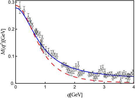
Figure 1: Blue solid line and red dashed line correspond to the MMF and ADFM quark–propagator Ansätze, respectively. Lattice data [84] are represented by the open triangles.

Euclidean formalism adopted in Ref. [20] avoids probation of the quark dressing functions (6) near their poles, $x=-a_{j}^{2}$, $j=1,2,3$. As we want to analytically continue $\sigma$’s to the complex plane and use these functions for the calculation in Minkowski space, a prescription for the pole treatment ought to be defined. An obvious choice is Feynman’s $i\varepsilon$ prescription, already used in the MMF–Ansatz case (2a); we push the poles infinitesimally from the real axis: $x=-a_{j}^{2}+i\varepsilon$, $j=1,2,3$. We use this prescription throughout this paper.

Functions $A(x)$ and $B(x)$ that follow from Eqs. (6) are also rational functions, exhibiting real poles for $x<0$. For example, Eqs. (1) imply that function $B$, which will be used in further calculation, is

$$B(x) =\frac{\sigma_{S}(x)}{\sigma_{S}^{2}(x)+x\,\sigma_{V}^{2}(x)}$$

$$=-\frac{\mathfrak{c}}{{\mathfrak{b}}_{1}-{\mathfrak{b}}_{2}}\left[\frac{({\mathfrak{b}}_{1}-{\mathfrak{a}})}{(x+{\mathfrak{b}}_{1})}+\frac{({\mathfrak{a}}-{\mathfrak{b}}_{2})}{(x+{\mathfrak{b}}_{2})}\right]~{},$$ (8)

where the coefficients ${\mathfrak{a}}$, ${\mathfrak{b}}_{1}$, ${\mathfrak{b}}_{2}$, and ${\mathfrak{c}}$ are some complicated algebraic functions of the original parameters $Z_{2}$, $a_{j}$, and $r_{j}$, appearing in Eqs. (6). Their calculated values are ${\mathfrak{a}}=38.1104~{}\unit{}^{2}$, ${\mathfrak{b}}_{1}=0.488784~{}\unit{}^{2}$, ${\mathfrak{b}}_{2}=2.65383~{}\unit{}^{2}$, and ${\mathfrak{c}}=-0.0178316~{}\unit{}^{3}$. A small $i\varepsilon$ shift of $\sigma_{V}$ and $\sigma_{S}$ poles, $x=-a_{j}^{2}+i\varepsilon$, $j=1,2,3$, causes the similar shift of the $B$ poles, $x=-{\mathfrak{b}}_{k}+i\varepsilon^{\prime}$, $k=1,2$, in agreement with the Feynman prescription.

For $z\in\mathbb{C}$ and large $|z|$ we find that $M(z)\propto 1/z$, but this asymptotic behavior is reached only at very high momenta squared, $|z|\simeq 1000~{}\unit{}^{2}$. The MMF quark–propagator Ansatz shows the same asymptotics for $m_{0}=0$, while $M(z)\sim m_{0}$ for $m_{0}\neq 0$; see Eq. (3). A well–known QCD result [85, 86] for the asymptotics of the quark mass function is

$$M(z)\propto\left\{\begin{array}[]{cc}{}[\log(z/\Lambda_{\mbox{\rm\scriptsize QCD}}^{2})]^{d-1}/z&\mbox{in the chiral limit}\\ {}[\log(z/\Lambda_{\mbox{\rm\scriptsize QCD}}^{2})]^{-d}&\mbox{otherwise}\end{array}\right.~{},$$ (9)

where $d=12/(11N_{c}-2N_{f})$ is the anomalous mass dimension, $N_{c}$ and $N_{f}$ are the number of colors and flavors, respectively and $\Lambda_{\mbox{\rm\scriptsize QCD}}\sim 0.5~{}\unit{}$ is the QCD scale. The simple meromorphic Ansätze, Eqs. (6) and (2), emulate the chiral–limit and away–from–the–chiral–limit behavior, respectively, of the quark mass function (9), up to the logarithmic corrections present in Eq. (9). The Ansätze are fitted to the respective lattice data: MMF quark propagator to lattice data of Ref. [84] and ADFM quark propagator to lattice data in the overlap [87, 88, 89] and asqtad (tadpole improved staggered) [90] formulations.

IV Pion decay constant

The pion decay constant $f_{\pi}$ is defined by the matrix element

$$\langle 0|\bar{d}(x)\gamma^{\mu}\gamma_{5}u(x)|\pi^{+}(P)\rangle=i\sqrt{2}f_{\pi}P^{\mu}e^{-iP\cdot x}~{},$$ (10)

where $u(x)$ and $d(x)$ are the quark fields (see, e.g., Ref. [2], Sec. 71.1). This matrix element is the hadronic part of the amplitude for $\pi^{+}\to l^{+}\nu_{l}$ decay, pictorially represented in Fig. 2. More explicitly, $f_{\pi}$ can be expressed in terms of the BS vertex function $\Gamma_{\pi}(q,P)$,

$$f_{\pi} =i\frac{N_{c}}{2M_{\pi}^{2}}$$

$$\times\int\frac{d^{4}q}{(2\pi)^{4}}\mbox{\rm tr}\left(\not{P}\gamma_{5}S(q+\frac{P}{2})\Gamma_{\pi}(q,P)S(q-\frac{P}{2})\right)~{},$$ (11)

where $N_{c}=3$ is the number of colors, and $M_{\pi}$ is the pion mass. Dictated by dynamical chiral symmetry breaking the axial–vector Ward–Takahashi identity, taken in the chiral limit, gives us the quark–level Goldberger–Treiman relation for the BS vertex,

$$\Gamma_{\pi}(q,P)\simeq-\frac{2B(-q^{2})_{\mbox{\rm\scriptsize c.l.}}}{f_{\pi}}\,\gamma_{5}~{},$$ (12)

which expresses $\Gamma_{\pi}$ in terms of the chiral–limit (c.l.) value of the quark dressing function $B$; see, e.g., Ref. [22]. This approximation will be used throughout this paper. [Note that it is the same approximation as in Ref. [19], as can be seen easily in spite of different notations and conventions, by comparing their Eqs. (18), (19) and (21) with our Eqs. (12) and (20). See also our Appendix.]

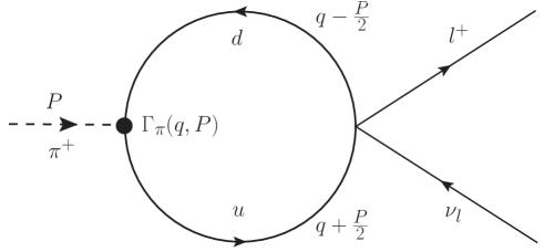
Figure 2: Diagram for $\pi^{+}\to l^{+}\nu_{l}$ decay.

The pion decay constant $f_{\pi}$ corresponding to the MMF quark–propagator model (2) has been calculated in three different ways: (a) analytically using Mathematica packages FeynCalc 9.0 [91, 92] and PACKAGE-X 2.0 [93, 94], (b) numerical integration in the Euclidean space, and (c) Minkowski space integration utilizing light-cone momenta and analytic residua calculation. Let us explain them in more detail.

(a) Using FeynCalc it is possible to express $f_{\pi}$ as a sum of terms containing Passarino-Veltman functions $B_{0}$ [95] of various arguments. PACKAGE-X is subsequently used for the final numerical evaluation, giving $f_{\pi}=87.5599~{}\unit{}$. The same result is obtained using LoopTools 2.0 [96] for the final numerical evaluation.

(b) The naive prescription for Wick rotation ($q^{0}\to-iq^{4}$, $\int dq^{0}\to i\int dq^{4}$) is justified here, for this specific propagator and for the pion decay constant calculation. Numerical integration in Euclidean space gives again the same $f_{\pi}$, to at least six significant digits. The four–dimensional integration is effectively two–dimensional, two integrations are trivial due to symmetry. The pion mass is taken to be $M_{\pi}=135~{}\unit{}$.

(c) Alternatively, following the procedure used in Ref. [19], integral (11) is calculated introducing light–cone variables $q_{\pm}=q^{0}\pm q^{3}$. The integrand is a rational function in $q_{-}$ variable, with seven simple poles on the real $q_{-}$ axis. Cauchy’s residue theorem is used to calculate the integral over $q_{-}$, paying attention to the $i\varepsilon$ rule for the displacement of poles, prescribed by Eq. (2a). The remaining two–dimensional integration over $q_{+}\in[-M_{\pi}/2,M_{\pi}/2]$ and $(q^{1})^{2}+(q^{2})^{2}$ is performed numerically. Eventually, the resulting $f_{\pi}=87.5599~{}\unit{}$ is in agreement with our previous calculations. The result of Ref. [19] is $f_{\pi}=90~{}\unit{}$, a little above our calculated value.

Regarding the ADFM Ansatz, $f_{\pi}$ is calculated using methods (a) and (b) mentioned above, and (d). Method (d) is the Minkowski space integration where the first integration, over $q^{0}$, boils down to residua calculation, as the principal value vanishes. All three methods give the same result, $f_{\pi}=71.5611~{}\unit{}$. Regarding the method (a), the trace appearing in Eq. (11) is evaluated using FeynCalc and LoopTools Mathematica packages, formally treating $B(x)$ as a sum of two propagators [see Eq. (8)].

V Electromagnetic form factor

The charged pion EMFF $F_{\pi}(Q^{2})$ is given by

$$\langle\pi^{+}(P^{\prime})|J^{\mu}(0)|\pi^{+}(P)\rangle=\mathcal{Q}_{\pi^{+}}(P^{\mu}+P^{\prime\mu})F_{\pi}(Q^{2})$$

$$=i(\mathcal{Q}_{u}-\mathcal{Q}_{d})\frac{N_{c}}{2}\int\frac{d^{4}q}{(2\pi)^{4}}\mbox{\rm tr}\Bigl{\{}\bar{\Gamma}_{\pi}(q-\frac{P}{2},P^{\prime})$$

$$\times S(q+\frac{1}{2}(P^{\prime}-P))\Gamma^{\mu}(q+\frac{1}{2}(P^{\prime}-P),q-\frac{1}{2}(P^{\prime}-P))$$

$$\times S(q-\frac{1}{2}(P^{\prime}-P))\Gamma_{\pi}(q-\frac{1}{2}P^{\prime},P)S(q-\frac{1}{2}(P+P^{\prime}))\Bigr{\}}~{},$$ (13)

in the generalized impulse approximation (GIA) [97, 98, 99], for spacelike $Q^{2}$, and the momentum routing as depicted in Fig. 3. The electromagnetic current is $J^{\mu}(x)$; the quark charge $\mathcal{Q}_{u}=2/3$ and $\mathcal{Q}_{d}=-1/3$. We use the following kinematics: $k=(0,0,0,\sqrt{Q^{2}})$, $P=(E_{\pi},0,0,-{\sqrt{Q^{2}}}/{2})$, and $P^{\prime}=(E_{\pi},0,0,\allowbreak{\sqrt{Q^{2}}}/{2})$, where $E_{\pi}=\sqrt{M_{\pi}^{2}+{Q^{2}}/{4}}$ and $Q^{2}\geq 0$. The Ball–Chiu vertex [100, 101] is used for the quark–quark–photon coupling throughout this paper,

$$\Gamma^{\mu}(p^{\prime},p)=\frac{1}{2}[A(-p^{\prime 2})+A(-p^{2})]\gamma^{\mu}+\frac{(p^{\prime}+p)^{\mu}}{(p^{\prime 2}-p^{2})}$$

$$\times\Bigr{\{}[A(-p^{\prime 2})-A(-p^{2})]\frac{\textstyle(\not{p}^{\prime}+\not{p})}{2}-[B(-p^{\prime 2})-B(-p^{2})]\Bigr{\}}~{}.$$ (14)

This vertex can be expressed completely in terms of the quark–propagator dressing functions and it becomes particularly simple in the case of the MMF Ansatz:

$$\Gamma^{\mu}(p^{\prime},p)=\gamma^{\mu}-\frac{m^{3}(p^{\prime\mu}+p^{\mu})}{(p^{\prime 2}-\lambda^{2}+i\varepsilon)(p^{2}-\lambda^{2}+i\varepsilon)}~{}.$$ (15)

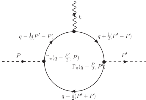
Figure 3: Impulse approximation to the charged pion electromagnetic form factor $F_{\pi}(Q^{2})$.

Similarly to the case of $f_{\pi}$ calculation, three methods are used to calculate $F_{\pi}(Q^{2})$ using the MMF Ansatz: (a) FeynCalc and PACKAGE-X Mathematica packages, (b) numerical integration in Euclidean space using adaptive quadrature, and (c) Minkowski space integration utilizing light–cone momenta and analytic residua calculation. Let us discuss these methods in more detail.

(a) $F_{\pi}(Q^{2})$, given by Eq. (13), is calculated using FeynCalc and PACKAGE-X Mathematica packages analogously to the $f_{\pi}$ calculation. The results are represented in Fig. 4.

(b) Numerical integration is performed using adaptive quadrature: expressing the space part of the four-vector $q$ in spherical coordinates, $q=(q^{0},\xi\sin\vartheta\cos\varphi,\allowbreak\xi\sin\vartheta\sin\varphi,\allowbreak\xi\cos\vartheta)$, the poles of the integrand, in variable $q^{0}$, are

$$(q^{0})_{1,2} =\mp\sqrt{M_{q}^{2}+\xi^{2}-\xi\sqrt{Q^{2}}\cos\vartheta+Q^{2}/4}~{},$$ (16a)

$$(q^{0})_{3,4} =\mp\sqrt{M_{q}^{2}+\xi^{2}+\xi\sqrt{Q^{2}}\cos\vartheta+Q^{2}/4}~{},$$ (16b)

$$(q^{0})_{5,6} =\frac{1}{2}\left(\sqrt{4M_{\pi}^{2}+Q^{2}}\mp 2\sqrt{M_{q}^{2}+\xi^{2}}\right)~{},$$ (16c)

$$(q^{0})_{7,8} =\frac{1}{4}\bigg{(}\sqrt{4M_{\pi}^{2}+Q^{2}}$$

$$\mp\sqrt{16M_{q}^{2}+16\xi^{2}+8\xi\sqrt{Q^{2}}\cos\vartheta+Q^{2}}\bigg{)}~{},$$ (16d)

$$(q^{0})_{9,10} =\frac{1}{4}\bigg{(}\sqrt{4M_{\pi}^{2}+Q^{2}}$$

$$\mp\sqrt{16M_{q}^{2}+16\xi^{2}-8\xi\sqrt{Q^{2}}\cos\vartheta+Q^{2}}\bigg{)}~{},$$ (16e)

where $M_{q}^{2}\in\{\mathfrak{p_{1}},\mathfrak{p_{2}},\mathfrak{p_{3}},\lambda^{2}\}$. The numbers $(-M_{q}^{2})$ are poles of the propagator functions (5) and (2a). Changing $M_{q}^{2}\to M_{q}^{2}-i\varepsilon$ pushes odd–indexed poles to the complex upper half–plane and even-indexed poles to the lower half–plane. We define two sets,

$${\cal A} =\Big{\{}(q^{0})_{j}\Big{|}j=1,3,5,7,9\land M_{q}^{2}=\mathfrak{p}_{1},\mathfrak{p}_{2},\mathfrak{p}_{3},\lambda^{2}\Big{\}}~{},$$ (17a)

$${\cal B} =\Big{\{}(q^{0})_{j}\Big{|}j=2,4,6,8,10\land M_{q}^{2}=\mathfrak{p}_{1},\mathfrak{p}_{2},\mathfrak{p}_{3},\lambda^{2}\Big{\}}~{},$$ (17b)

where ${\cal A}$ and $\cal B$ contain poles that must be bypassed from below and from above, respectively. Note that not all four values of $M_{q}^{2}$ produce poles of the integrand. For example, $(q^{0})_{7,8}$ are poles of the integrand only for $M_{q}^{2}=\lambda^{2}$; these two poles correspond to singular behavior of $\Gamma_{\pi}(q-P/2,P^{\prime})$ and are defined by equation $(q-P/2)^{2}=\lambda^{2}$. For simplicity of definition, sets ${\cal A}$ and ${\cal B}$ are allowed to contain superfluous points, but this does not obstruct the analysis hereafter. Numerical examination shows that $\max\{{\cal A}\}<\min\{{\cal B}\}$ for the chosen model parameters, so we define

$$(q^{0})_{c}=\frac{1}{2}\left(\max\{{\cal A}\}+\min\{{\cal B}\}\right)~{},$$ (18)

which is a function of $\vartheta$ and $\xi$, but does not depend on $\varphi$ thanks to the symmetry. Figure  5 illustrates the $\xi$ dependence of $(q^{0})_{j}$’s and $(q^{0})_{c}$ for a fixed value of $\vartheta$. Unlike the case of the $f_{\pi}$ calculation (11), where the first and third quadrants of the $q^{0}$ complex plane is free of poles and the naive Wick rotation $q^{0}=-iq_{4}$ ($q_{4}\in\mathbb{R}$) is allowed, in the present case of the $F_{\pi}(Q^{2})$ calculation, the path of integration ought to be shifted to pass between poles contained in the ${\cal A}$ and ${\cal B}$,

$$q^{0}=(q^{0})_{c}-iq_{4}~{},$$ (19)

where $q_{4}\in\langle-\infty,\infty\rangle$. Eventually, the numerical integration over $q_{4}$, $\xi$, and $\vartheta$ is performed using the adaptive quadrature; see Fig. 4 for the final result.

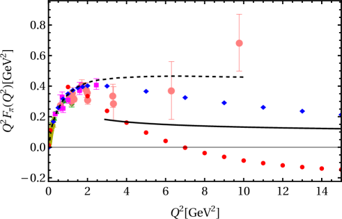
Figure 4: Charged pion electromagnetic form factor. Experimental points are shown by dark yellow triangles [102], green diamonds [103], pink circles [104, 105, 106], and magenta squares [107, 108, 109, 110]. Red solid circles and blue diamonds are calculated using the ADFM quark–propagator Ansatz and the MMF quark–propagator Ansatz, respectively. In the case of the MMF quark propagator, three different methods of calculation (detailed in the text) yielded the same results. The black dashed line represents the result of Mello et al. [19]. The black solid line corresponds to the perturbative QCD result (27) with asymptotic PDA.

(c) Minkowski space integration utilizing light-cone momenta is again performed analogously to the $f_{\pi}$ calculation. Now, there are 11 poles, in variable $q_{-}$, of the integrand of Eq. (13). The residua are calculated analytically and adaptive quadrature is used for the final three–dimensional integration.

To conclude about the EMFF obtained with the MMF Ansatz, there are only insignificant differences, of order $\lesssim 0.1\%$, between results for $F_{\pi}(Q^{2})$ calculated using methods (a), (b), and (c). The differences are compatible with the precision of numerical integration that we prescribed in methods (b) and (c). However, there is a significant discrepancy between our results (blue dots) and those of Ref. [19] (black dashed line in our Fig. 4). The MMF Ansatz [19] is also used in Ref. [111], with the same model parameter values. While $Q^{2}F_{\pi}(Q^{2})$ is practically constant for $Q^{2}\gtrsim 3~{}\unit{}^{2}$ in the former paper, it falls with $Q^{2}$ very noticeably in the latter one. Hence, Ref. [111] agrees better with our EMFF, although it still falls more slowly than ours.

For the ADFM quark propagator, we have calculated $F_{\pi}(Q^{2})$ using only one method out of three adopted for the MMF Ansatz; namely, method (b), the modified Wick rotation, defined by Eq. (19), and subsequent three–dimensional adaptive Monte Carlo integration. The results are depicted as red solid circles in Fig. 4.

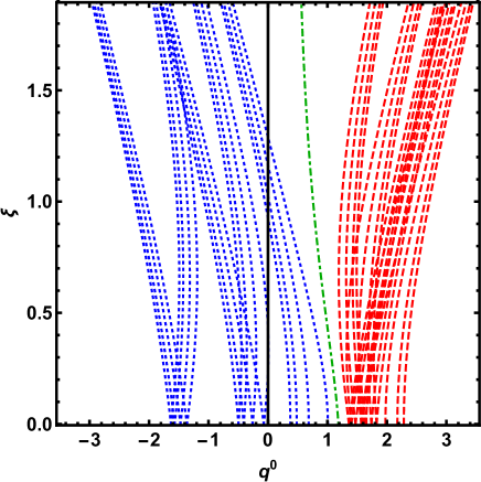
Figure 5: $(q^{0})_{j}$’s and $(q^{0})_{c}$ vs. $\xi$ for $\vartheta=\pi/3$ and $Q^{2}=7~{}\unit{}^{2}$. All in units of GeV. Dot–dashed green line represents $(q^{0})_{c}$, blue dotted lines represent odd-indexed poles (set ${\cal A}$), and red dashed lines represents even–indexed poles (set ${\cal B}$).

Concerning the low–$Q^{2}$ behavior, the pion charge radius $r_{\pi}=\sqrt{-6F_{\pi}^{\prime}(0)}$ is calculated to be $r_{\pi}=0.632~{}\mbox{\rm fm}$ and $0.699~{}\mbox{\rm fm}$ for MMF and ADFM Ansätze, respectively. Both values are reasonably near the experimental value of $r_{\pi}=(0.659\pm 0.004)~{}\mbox{\rm fm}$ [2]. The simple constituent quark model formula $r_{\pi}=\sqrt{3}/(2\pi f_{\pi})$ [112, 113] gives $r_{\pi}=0.621~{}\mbox{\rm fm}$ and $0.760~{}\mbox{\rm fm}$ for MMF and ADFM Ansätze, respectively. The approximate BS vertex (12) does not guarantee that the normalization condition $F_{\pi}(0)=1$ will be fulfilled. The general form of the pseudoscalar BS vertex is

$$\Gamma_{\pi}(q,P)=\gamma_{5}\Bigl{(}H_{1}(q,P)$$

$$+\not{P}H_{2}(q,P)+\not{q}H_{3}(q,P)+[\not{P},\not{q}]H_{4}(q,P)\Bigr{)}~{},$$ (20)

where $H_{1}$, $H_{2}$, $H_{3}$, and $H_{4}$ are Lorentz–scalar functions [114]. Solely keeping $H_{1}$ component and neglecting others, just as we do in Eq. (12), leads to deviation from $F_{\pi}(0)=1$ normalization condition [115]. We obtain $F_{\pi}(0)=0.950$ and $1.32$ for MMF and ADFM Ansätze, respectively [which is interesting to compare, but of course we could also follow Ref. [19], which forces $F_{\pi}(0)=1$ by adjusting the normalization of BS vertex (20); for more details see Appendix A.]

The high–$Q^{2}$ asymptotics of the charged pion EMFF is discussed in Sec. VII along with the asymptotics of the neutral pion TFF, which is introduced in the next section.

VI Transition form factor

The two–photon amplitude $T(k^{2},k^{\prime 2})$ that describes $\pi^{0}\to\gamma\gamma^{(\star)}$ processes, depicted in Fig. 6, is given by

$$T^{\mu\nu}(k,k^{\prime})=\varepsilon^{\mu\nu\lambda\sigma}k_{\lambda}k^{\prime}_{\sigma}T(k^{2},k^{\prime 2})$$

$$=-N_{c}\,\frac{\mathcal{Q}_{u}^{2}-\mathcal{Q}_{d}^{2}}{2}\int\frac{d^{4}q}{(2\pi)^{4}}\mbox{\rm tr}\Bigl{\{}\Gamma^{\mu}(q-\frac{P}{2},k+q-\frac{P}{2})$$

$$\times S(k+q-\frac{P}{2})\Gamma^{\nu}(k+q-\frac{P}{2},q+\frac{P}{2})S(q+\frac{P}{2})$$

$$\times\Gamma_{\pi}(q,P)S(q-\frac{P}{2})\Bigr{\}}+(k\leftrightarrow k^{\prime},\mu\leftrightarrow\nu)~{},$$ (21)

in the GIA [63, 64, 13], where $k$ and $k^{\prime}$ are the external photon momenta, $P=k+k^{\prime}$ is the neutral pion momentum, and $P^{2}=M_{\pi}^{2}$. The TFF is defined as

$$F_{\pi\gamma}(Q^{2})=|T(-Q^{2},0)|~{},$$ (22)

such that the $\pi^{0}\to\gamma\gamma$ decay width can be written as

$$\Gamma(\pi^{0}\to\gamma\gamma)=\frac{\pi\alpha^{2}M_{\pi}^{3}}{4}F_{\pi\gamma}(0)^{2}~{}.$$ (23)

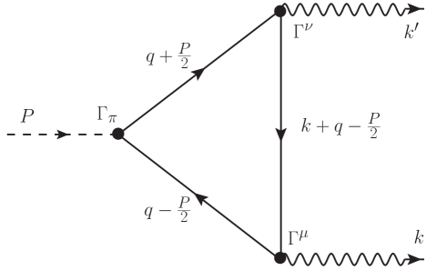
Figure 6: The quark triangle diagram for the transition form factor calculation.

In respect of the MMF Ansatz, the FeynCalc package is used to express the loop integral in Eq. (21) as a sum of the Passarino–Veltman functions, while PACKAGE-X is used for the final numerical evaluation, in a close analogy to the $F_{\pi}(Q^{2})$ calculation, Sec. V, method (a). The results of our calculation are pictorially represented by the blue dots in Fig. 7. The experimental results are shown as solid circles and diamonds (with error bars) in the same figure.

On the other hand, the case of the ADFM Ansatz is treated solely using method (b) described in Sec. V. The integrand appearing in Eq. (21), as a function of $q^{0}$, exhibits the same structure of the pole trajectories in the $q^{0}\xi$–plane, as those illustrated in Fig. 5 in the case of EMFF calculation. The results are represented by the red pluses in Fig. 7.

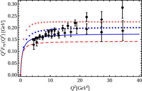
Figure 7: Blue dots represent $\pi^{0}$ transition form factor calculated using the MMF quark–propagator Ansatz, Eqs. (1) and (2). The red pluses are calculated using the ADFM quark propagator, Eqs. (6). The blue solid line and red dashed line represent the Brodsky–Lepage interpolation formula (29), for the MMF quark–propagator and ADFM quark–propagator models, respectively. Solid circles and diamonds (with error bars) represent the measurements of BaBar [116] and Belle [117] Collaborations, respectively.

It has been shown in Refs. [118, 63] that the GIA amplitude (21) gives $F_{\pi\gamma}(0)=1/(4\pi^{2}f_{\pi})$ in the chiral limit, regardless of the specific choice of the quark dressing functions $\sigma_{V}$ and $\sigma_{S}$, and in agreement with the Adler–Bell–Jackiw (ABJ) anomaly result [119, 120]. Our numerical results for $F_{\pi\gamma}(0)$ complies fairly to this limit; the deviations are about 4.3% and 0.7% for MMF and ADFM Ansätze, respectively.

The function $F_{\pi\gamma}(Q^{2})$ is expected to be a smooth function near $Q^{2}=0$, down to $Q^{2}=-M_{V}^{2}$ where the vector–meson resonance peaks appear; $V=\rho,\omega,\phi,\dots$. The slope parameter $a$ is defined through the expansion of the (normalized) TFF,

$$\frac{F_{\pi\gamma}(Q^{2})}{F_{\pi\gamma}(0)}=1-a\,\frac{Q^{2}}{M_{\pi}^{2}}+{\cal}O((Q^{2})^{2})~{}.$$ (24)

The recent experimental result of the NA62 Collaboration is $a=0.0368\pm 0.0057$ [121]; the A2 Collaboration at MAMI gives $a=0.030\pm 0.010$ [122]. In both experiments, the Dalitz decay $\pi^{0}\to e^{+}e^{-}\gamma$ is measured for low timelike momentum transfer: $-M_{\pi}^{2}\leq Q^{2}=(p_{e^{-}}+p_{e^{+}})^{2}\leq-4m_{e}^{2}$. Our calculation gives $a=-M_{\pi}^{2}\,F_{\pi\gamma}^{\prime}(0)/F_{\pi\gamma}(0)=0.027$ for MMF Ansatz and $a=0.025$ for ADFM Ansatz, in reasonable agreement with the experimental values. The following method was used to determine $a$. We calculated several $(Q^{2},F_{\pi\gamma}(Q^{2}))$ points in the interval $-0.3~{}\unit{}^{2}\leq Q^{2}\leq 0.3~{}\unit{}^{2}$ and $-0.2~{}\unit{}^{2}\leq Q^{2}\leq 0.2~{}\unit{}^{2}$ for MMF and ADFM Ansatz, respectively. These points were fitted to $F_{\pi\gamma}(Q^{2})=A/(1+Q^{2}/B^{2})$ curve; the derivative $F_{\pi\gamma}^{\prime}(0)$ was computed from this fit. A simple quark triangle model [123] gives $a={M_{\pi}^{2}}/(12M_{c}^{2})$, where $M_{c}$ is the constituent quark mass. Using $M_{\pi}=135~{}\unit{}$ and $M_{c}=M(0)=280~{}\unit{}$ (estimated from Fig. 1) gives $a=0.02$, somewhat below the experimental values and our model results. The high–$Q^{2}$ asymptotics of $F_{\pi\gamma}$ is addressed in the next section and is compared with those calculated from the PDA.

VII Pion distribution amplitude and asymptotics of form factors

The factorization property of the QCD hard scattering amplitudes enables us to express these amplitudes in terms of the pertinent distribution amplitudes. The PDA, relevant for the TFF and EMFF calculation at large $Q^{2}$, can be expressed as the light–cone projection,

$$\phi_{\pi}(u)=i\frac{N_{c}}{8\pi f_{\pi}}\mbox{\rm tr}\left(\gamma_{+}\gamma_{5}\int\frac{dq_{-}}{2\pi}\int\frac{d^{2}q_{\perp}}{(2\pi)^{2}}\,\chi_{\pi}(q,P)\right)~{},$$ (25)

of the BS amplitude

$$\chi_{\pi}(q,P)=S(q+\frac{P}{2})\Gamma_{\pi}(q,P)S(q-\frac{P}{2})$$ (26)

[124, 125, 126, 127, 128]. The variable $q_{+}$, which is implicit in the integrand of Eq. (25), is defined by $u=1/2+q_{+}/P_{+}$. The integral resembles those of the $f_{\pi}$–calculation (11) and could be treated in the same way. For both propagator Ansätze we use the Euclidean space integration, referred as method (b) in Secs. IV and V. The resulting PDAs are displayed in Fig. 8.

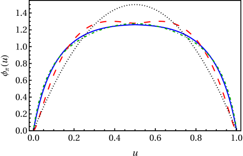
Figure 8: Pion distribution amplitudes $\phi_{\pi}(u)$. Blue solid line and red dashed line correspond to the MMF and ADFM Ansätze, respectively. Black dotted line represents the asymptotic form, $\phi_{\pi}^{\mbox{\rm\scriptsize as}}(u)=6u(1-u)$. Dash-dotted green line (very close to the solid blue one, and hardly discernible from it) is the PDA from the state-of-the-art SDE pion bound state, Eq. (22) in Ref. [9].

The leading twist pQCD results for the asymptotics of the pion form factor is [129, 130, 131, 132]

$$F_{\pi}(Q^{2})\sim\frac{16\pi\alpha_{s}(Q^{2})f_{\pi}^{2}}{Q^{2}}\left|\frac{1}{3}\int_{0}^{1}du\,\frac{\phi_{\pi}(u)}{u}\right|^{2}$$ (27)

for $Q^{2}\to\infty$, where $\alpha_{s}$ is the QCD running coupling constant: $\alpha_{s}(Q^{2})={d\pi}/{\ln(Q^{2}/\Lambda_{\mbox{\rm\scriptsize QCD}}^{2})}$ at the one–loop order of perturbation theory, while $d$ is the same as in Eq. (9). The renormalization scale ($\mu$) dependence of PDA is implicit here. The asymptotic form of PDA, $\phi_{\pi}^{\mbox{\rm\scriptsize as}}(u)=\lim_{\mu\to\infty}\phi_{\pi}(u)\allowbreak=\allowbreak 6u(1-u)$, gives $\frac{1}{3}\int du\,\phi_{\pi}^{\mbox{\rm\scriptsize as}}(u)/u=1$, leading to $F_{\pi}(Q^{2})\sim{16\pi\alpha_{s}(Q^{2})f_{\pi}^{2}}/{Q^{2}}$ asymptotic behavior. The PDAs $\phi_{\pi}(u)$, related to the models under consideration, do not deviate too much from the asymptotic $\phi_{\pi}^{\mbox{\rm\scriptsize as}}(u)$ function; see Fig. 8. The actual values of integrals are $\frac{1}{3}\int du\,\phi_{\pi}(u)\allowbreak/u=$ $1.15$ and $1.02$ for the MMF and ADFM models, respectively. This results in respective 32% and 4% enhancement of $F_{\pi}(Q^{2})$ relative to value obtained with $\phi_{\pi}^{\mbox{\rm\scriptsize as}}$.

The asymptotic form of EMFF (27), being dependent on $\alpha_{s}(Q^{2})$, critically reflects the perturbative nature of high–energy QCD. Our simple meromorphic Ansätze (2) and (6), which do not comply with the exact QCD asymptotics (9), is not expected to reproduce the UV logarithmic behavior of Eq. (27). We computed $F_{\pi}(Q^{2})$ up to $Q^{2}=40~{}\unit{}^{2}$ and indeed found no evidence that the asymptotic behavior $F_{\pi}(Q^{2})\propto 1/(Q^{2}\ln(Q^{2}))$ was reached, for either of our models. The presently available experimental data on $F_{\pi}(Q^{2})$ are anyway well above the pQCD predictions (27), as discussed in Ref. [133] in more detail.

The same PDA (25) also determines the leading term of the light–cone expansion of form factor $F_{\pi\gamma}(Q^{2})$ [126, 134],

$$F_{\pi\gamma}(Q^{2})\sim\frac{2f_{\pi}}{3Q^{2}}\int_{0}^{1}\frac{du\,\phi_{\pi}(u)}{(1-u)}~{}.$$ (28)

The asymptotic form of the PDA leads to $F_{\pi\gamma}(Q^{2})\sim 2f_{\pi}/Q^{2}$ for $Q^{2}\to\infty$ asymptotic behavior [126, 135]. The Brodsky–Lepage (BL) dipole formula [135],

$$F_{\pi\gamma}(Q^{2})=\frac{1}{4\pi^{2}f_{\pi}}\left(1+\frac{Q^{2}}{8\pi^{2}f_{\pi}^{2}}\right)^{-1}~{},$$ (29)

interpolates between $F_{\pi\gamma}(0)=1/(4\pi^{2}f_{\pi})$, the ABJ anomaly result [119, 120], and $\lim_{Q^{2}\to\infty}Q^{2}F_{\pi\gamma}(Q^{2})=2f_{\pi}$, the pQCD limit. The current experimental data [116, 117], reaching up to $Q^{2}\sim 35~{}\unit{}^{2}$, do not show agreement with this limit yet. On the theoretical side, recent SDE studies in Euclidean space are not unanimous: Raya et al. [68] are consistent with the hard scattering limit, but Eichmann et al. [136] claim that the BL limit is modified whenever the other external photon is near on shell, i.e, $k^{\prime 2}\simeq 0$. That is, some nonperturbative effects would always persist in this case. The modified BL limit is also claimed independently from the SDE approach, by some quite different theoretical studies [137, 138, 139].

As we can see from Fig. 7 and Table 1, the high–$Q^{2}$ behavior of $F_{\pi\gamma}(Q^{2})$ calculated in the GIA (21) deviates appreciably from the BL limit of $2f_{\pi}/Q^{2}$ for both model Ansätze. GIA limit of $F_{\pi\gamma}(Q^{2})$ overshoots BL limit by 58% and 15% for ADFM and MMF models, respectively.

approximation	ADFM		MMF
GIA	$0.225\,96$	($0.226\,306$)	$0.201\,817$	($0.200\,065$)
bare	$0.145\,45$	($0.140\,809$)	$0.200\,458$	($0.187\,294$)
BL-non-asymptotic	$0.146\,308$		$0.201\,797$
BL	$0.143\,12$		$0.175\,120$

Table 1: $\lim_{Q^{2}\to\infty}Q^{2}F_{\pi\gamma}(Q^{2})$, in units of GeV, calculated using various approximation schemes. The first two rows (denoted by GIA and bare), when related to the ADFM Ansatz, are computed by fitting the function $Q^{2}\mapsto\kappa_{0}+\kappa_{1}/Q^{2}$ to a set of discrete values of $Q^{2}F_{\pi\gamma}(Q^{2})$ calculated in the interval $10~{}\unit{}^{2}\leq Q^{2}\leq 50~{}\unit{}^{2}$. The symbols $\kappa_{n}$ $(n=0,1,2,3)$ denote the fitting constants. In the MMF case, the corresponding limits are computed by fitting the function $Q^{2}\mapsto\kappa_{0}+\kappa_{1}/Q^{2}+\kappa_{2}/(Q^{2})^{2}+\kappa_{3}/(Q^{2})^{3}$ to values of $Q^{2}F_{\pi\gamma}(Q^{2})$ calculated in the interval $20~{}\unit{}^{2}\leq Q^{2}\leq 100~{}\unit{}^{2}$. Thus, $\lim_{Q^{2}\to\infty}Q^{2}F_{\pi\gamma}(Q^{2})=\kappa_{0}$ for both GIA and bare rows, for the both Ansätze. In the brackets are the results of the same GIA and bare calculations obtained at $\,Q^{2}=40\unit{}^{2}$, to illustrate the differences between $\,Q^{2}F_{\pi\gamma}(Q^{2})$ at a large but finite $\,Q^{2}$ and in the $\,Q^{2}\to\infty$ limit. The last two rows are calculated from Eq. (28), using the appropriate PDAs. Thus, the fourth row is simply $\,2f_{\pi}$ due to $\phi_{\pi}(u)=\phi_{\pi}^{\mbox{\rm\scriptsize as}}(u)$. However, the third row differs from $\,2f_{\pi}$, since PDAs used in Eq. (28) are not asymptotic, but calculated in the MMF and ADFM models through Eq. (25).

The row denoted by “bare” in Table 1 is calculated from Eq. (21) by replacing the dressed electromagnetic vertices $\Gamma^{\mu}(q,q^{\prime})$ with the bare ones $\gamma^{\mu}$ and the quark propagators $S(l)$ that propagate hard momenta $l=q\pm(k-k^{\prime})/2$, with the bare (and massless) ones, $\not{l}/l^{2}$. This leads to a much simpler expression for $T^{\mu\nu}$:

$$T^{\mu\nu}(k,k^{\prime})=-2iN_{c}\,\frac{\mathcal{Q}_{u}^{2}-\mathcal{Q}_{d}^{2}}{2}\,\varepsilon^{\mu\nu\lambda\sigma}\,$$

$$\times\int\frac{d^{4}q}{(2\pi)^{4}}\frac{\left[\frac{1}{2}(k^{\prime}-k)-q\right]_{\lambda}}{\left[\frac{1}{2}(k^{\prime}-k)-q\right]^{2}}\,\mbox{\rm tr}\{\gamma_{\sigma}\gamma_{5}\chi_{\pi}(q,P)\}~{}.$$ (30)

The pertaining $\lim_{Q^{2}\to\infty}Q^{2}F_{\pi\gamma}(Q^{2})$ deviates negligibly from the corresponding GIA value in the case of the MMF Ansatz, but the deviation is significant in the case of the ADFM Ansatz.

It is apparent that not all quark legs attached to electromagnetic vertices carry the large momentum scale $Q^{2}$ ; see Fig. 6. It is enough to improve the previous bare approximation (30) such that we partially restore these soft contributions originally present in the Ball–Chiu vertex (14),

$$\gamma^{\mu(\nu)}\to\frac{1}{2}\left(1+A\Bigl{(}-[q-(+)\frac{P}{2}]^{2}\Bigr{)}\right)\gamma^{\mu(\nu)}~{},$$ (31)

and the GIA limit is recovered [13, 140],

$$\lim_{Q^{2}\to\infty}Q^{2}F^{\mbox{\rm\scriptsize``$(1+A_{\mbox{\rm\scriptsize soft}})/2$''}}_{\pi\gamma}(Q^{2})=0.225~{}\unit{}~{},$$ (32)

where the superscript “$(1+A_{\mbox{\rm\scriptsize soft}})/2$” indicates that $F_{\pi\gamma}$ is calculated using vertex (31) instead of the Ball–Chiu one. Hence, the nontrivial infrared behavior of the wave function renormalization $Z(x)=1/A(x)\neq 1$ is responsible for the two calculations, the first one based on GIA Eq. (21) and the second one based on bare Eq. (30), producing unequal asymptotics of $F_{\pi\gamma}(Q^{2})$. Of course, for the MMF Ansatz, where $Z(x)\equiv 1$, both calculations give the same asymptotic limit.

The respective integral $\frac{1}{3}\int du\,\phi_{\pi}(u)/u$ values of 1.02 and 1.15 for the MMF and ADFM Ansätze, which influence the EMFF asymptotics (27), are reflected also in the asymptotic behavior of the TFF calculated from Eq. (28) and shown in Table 1, in the row denoted by BL-non-asymptotic [for it is not calculated using the asymptotic form of $\phi(u)$, but the model calculated one].

To the end of this section, we explain the similarity between the bare and BL-non-asymptotic approximation. Light–cone expansion of the time–ordered product of two electromagnetic currents, $T\{J^{\mu}(x),J^{\nu}(y)\}$, leads to the following approximate expression:

$$T^{\mu\nu}(k,k^{\prime})\simeq 2\frac{\mathcal{Q}_{u}^{2}-\mathcal{Q}_{d}^{2}}{\sqrt{2}}\frac{1}{2\pi^{2}}\varepsilon^{\mu\nu\lambda\sigma}$$

$$\times i\int d^{4}z\,e^{ik^{\prime}\cdot z}\frac{z_{\lambda}}{z^{4}}\langle\mbox{\rm vac}|:\bar{d}(0)\gamma_{\sigma}\gamma_{5}u(z):|\pi^{+}(P)\rangle_{z^{2}=0}~{}.$$

(See, e.g., Refs. [144, 145].) The path–ordered “string operator,”

$$P\exp\left(ig\int_{x}^{0}A^{\alpha}(y)dy_{\alpha}\right)~{},$$ (34)

must be included between the quark fields. This operator equals unity in light–cone gauge; see, e.g., Ref. [125].

On the one hand, expressing the above $\pi^{+}$-to-vacuum matrix element through the the BS amplitude,

$$\langle\mbox{\rm vac}|:\bar{u}(0)\gamma^{\mu}\gamma_{5}u(z)-\bar{d}(0)\gamma^{\mu}\gamma_{5}d(z):|\pi^{0}(P)\rangle$$

$$=-N_{c}\,e^{-iP\cdot z/2}\int\frac{d^{4}q}{(2\pi)^{4}}e^{-iq\cdot z}\mbox{\rm tr}\left(\gamma^{\mu}\gamma_{5}\chi_{\pi}(q,P)\right)~{},$$ (35)

we reproduce bare Eq. (30). On the other hand, the definition of the PDA,

$$\frac{1}{2}\langle\mbox{\rm vac}|:\bar{u}(0)\gamma^{\mu}\gamma_{5}u(z)-\bar{d}(0)\gamma^{\mu}\gamma_{5}d(z):|\pi^{0}(P)\rangle_{z_{+}=z_{\perp}=0}$$

$$=i\delta^{ab}f_{\pi}P^{\mu}\int_{0}^{1}du\,e^{-iuP\cdot z}\,\phi_{\pi}(u)~{},$$ (36)

leads eventually to the BL-non-asymptotic approximation, Eq. (28). To conclude, both Eqs. (28) and (30) follow from Eq. (LABEL:PionDistributionAmplitude:Tmunu:LightCone), except Eq. (28) is derived without the $z^{2}=0$ constraint, i.e., without light-cone projection of the nonlocal operator ${:\bar{\psi}(0)\frac{\lambda^{a}}{2}\gamma^{\mu}\gamma_{5}\psi(z):}$. It turns out that such a difference is of little influence, at least for the models under consideration.

VIII Summary and conclusions

In this paper, we have studied two meromorphic Ansätze for the dressed quark propagator (suggested in Refs. [19] and [20]), which represent strongly nonperturbative dressing, but still permit formulating clear connections between Euclidean and Minkowski spacetime calculations. Thanks to the quark–level Goldberger–Treiman relation (12), the pseudoscalar BS vertex can be related to the dynamically dressed momentum–dependent quark mass function [22]. Additionally, by exploiting the Ball–Chiu vertex [100, 101] as an approximation for the fully dressed quark–quark–photon vertex, we are provided with all the necessary elements to calculate the pion decay constant, EMFF, TFF, and PDA. The related amplitudes were calculated using several methods in order to check the robustness of the results.

The used quark Ansätze as well as the pertaining vertices exhibit masslike singularities on the real timelike momentum axis and do not obey the pQCD asymptotic behavior; hence, we can hardly expect that the correct perturbative asymptotic behavior of the electromagnetic form factor $F_{\pi}(Q^{2})\propto 1/(Q^{2}\ln(Q^{2}))$ will be attained. Indeed, our numerical evaluation of $F_{\pi}(Q^{2})$ up to $Q^{2}=40~{}\unit{}^{2}$ did not show evidence that either $F_{\pi}(Q^{2})\sim 1/(Q^{2}\ln(Q^{2}))$ limit or simpler power–law $F_{\pi}(Q^{2})\allowbreak\sim 1/Q^{2}$ limit is reached. However, it should be acknowledged that the exact asymptotic behavior is of purely academic interest here because (a) it is generally expected that the asymptotic regime probably starts at $Q^{2}\gtrsim 20~{}\unit{}^{2}$, well above Jefferson Lab capability after proposed upgrade [146], (b) and even existing Cornell experimental data at $Q^{2}=6.30~{}\unit{}^{2}$ and $9.77~{}\unit{}^{2}$ have large error bars [106]. For high $Q^{2}$, our results for $Q^{2}F_{\pi}(Q^{2})$ obviously deviate from those of Ref. [19]. The low–$Q^{2}$ behavior of $F_{\pi}(Q^{2})$, encoded in the pion charge radius $r_{\pi}$, was found to be in a reasonable agreement with experiment, given the simplicity of the model.

The leading–order pQCD expression for the high–$Q^{2}$ behavior of the transition form factor, $F_{\pi\gamma}(Q^{2})\sim 2f_{\pi}/Q^{2}$, depends only on $f_{\pi}$, the low–energy pion observable, which is pretty insensitive to the details of the high–energy dynamics. Hence, we could naively expect that our Ansätze, despite not incorporating the exact perturbative regime behavior, should produce the correct perturbative limit of the pion transition form factor. However, in the generalized impulse approximation the electromagnetic vertices keep one quark leg soft, even for the high–$Q^{2}$ external photon. As the result, this approximation gave $Q^{2}F_{\pi\gamma}(Q^{2})$ finite for $Q^{2}\to\infty$, but, similar to Refs. [136, 137, 138, 139], generally unequal to the pQCD limit of $2f_{\pi}$; see also Refs. [13, 140]. In relation to low–$Q^{2}$ behavior, our results for the TFF slope parameter are 10%-15% below the experimental value.

The pion distribution amplitudes that were calculated using our Ansätze did not deviate appreciably from the asymptotic one. If we input these amplitudes (instead of the asymptotic one) to the pQCD form–factor formulae, the result is enhanced up to  30%, depending on the form factor and Ansätze. When one compares the results given above, the MMF Ansatz is considerably more successful than the ADFM one. In part, this can be explained by noticing that the PDA that we obtained from the MMF Ansatz (the solid curve in Fig. 8) is very close to the PDA calculated from the pion bound-state amplitude obtained using the most sophisticated SDE kernel [9]. This PDA is given by Eq. (22) in Ref. [9], and is hardly discernible from our solid curve in Fig. 8. This indicates that the MMF Ansatz at least partially captures the results obtained by some of the presently most advanced SDE calculations [9]. The MMF Ansatz (2) is more realistic also in that it incorporates the explicit chiral symmetry breaking, whereas the ADFM one (6) corresponds to the chiral limit, for which the ADFM paper [20] concludes that their parametrizations should yield values of the pion decay constant $f_{\pi}$ 10-20% below the empirical value. Their value is thus just $f_{\pi}=(71\pm 3)$ MeV [20], obtained for the presently adopted ADFM Ansatz and its parameters in Eq. (6). Hence, the large difference between MMF and ADFM results for $f_{\pi}$ is inherited from the respective Refs. [19, 20], since we adopted their respective Ansätze and parameters without change.

In the present paper, however, more important than the phenomenological considerations is the following: the simple analytic structure of quark–propagator Ansätze employed, together with suitable approximations for the required vertices, enabled us to keep control of the Wick rotation when calculating some processes; the pertinent amplitudes can be calculated equally in Minkowski and Euclidean space. Kindred studies are mostly restricted to the Euclidean space; their propagators and vertices are sensibly defined for spacelike external momenta, $q^{2}=(q^{0})^{2}-|\mbox{\boldmath$q$}|^{2}<0$, but their analytic properties (singularities in the first and third quadrants of the complex $q^{0}$ plane) preclude Wick rotation back to the Minkowski space. In principle, it is not difficult to impose the correct perturbative asymptotic behavior on gluon and quark propagators in such models. In the context of the coupled Schwinger–Dyson and Bethe–Salpeter equation, such an example is provided in Refs. [147, 148, 149]; a similar and widely used model is introduced in Refs. [150, 151] and its application reviewed in Ref. [152]. Among the variety of quark–propagator Ansätze explored in Ref. [20] that exhibit correct pQCD behavior, none is suitable for the calculation methods presented in this work: the branch cut in propagator functions do not allow the use of perturbative techniques while the complicated singularity structure prevents the Wick rotation.

Future work may include calculation of some other processes involving quark loops, e.g., $\gamma^{\star}\to 3\pi$, $\gamma\gamma\to\pi\pi$, and $\pi^{0}\to e^{-}e^{+}$. The most appealing improvement would be a quark propagator Ansatz that has the correct UV behavior and, at the same time, enough simple analytic structure that allow Wick rotation (in the sense used in this paper). But it is not evident to us whether such a task could be achieved.

Appendix A Normalization of the BS amplitude

The matrix element of the electromagnetic current is generally

$$\langle\pi^{+}(P^{\prime})|J^{\mu}(x)|\pi^{+}(P)\rangle=e^{-i(P^{\prime}-P)\cdot x}$$

$$\times\big{(}(P^{\mu}+P^{\prime\mu})F_{\pi}(Q^{2})+(P^{\mu}-P^{\prime\mu})G_{\pi}(Q^{2})\big{)}~{}.$$ (37)

The electromagnetic current conservation $\partial_{\mu}J^{\mu}(x)=0$ implies $G_{\pi}(Q^{2})=0$. Our pion states normalization,

$$\langle\pi^{+}(P^{\prime})|\pi^{+}(P)\rangle=(2\pi)^{3}\,2E(\mbox{\boldmath$P$})\,\delta^{(3)}(\mbox{\boldmath$P$}-\mbox{\boldmath$P$}^{\prime})~{},$$ (38)

where $E(\mbox{\boldmath$P$})=\sqrt{M_{\pi}^{2}+|\mbox{\boldmath$P$}|^{2}}$, together with

$$\hat{Q}|\pi^{+}(P)\rangle=\int d^{3}xJ^{0}(x)|\pi^{+}(P)\rangle=|\pi^{+}(P)\rangle$$ (39)

automatically ensures that

$$F_{\pi}(0)=1~{}.$$ (40)

In the chiral limit, the axial–vector Ward–Takahashi identity reads

$$(p^{\prime}-p)_{\lambda}\Gamma_{5}^{\,\,a\lambda}(p^{\prime},p)=\left(S^{-1}(p^{\prime})\gamma_{5}+\gamma_{5}S^{-1}(p)\right)\frac{\lambda^{a}}{2}~{}.$$ (41)

The pion pole contribution to the axial–vector vertex is

$$\Gamma_{5}^{\,\,a\lambda}(p^{\prime},p)\simeq\frac{\lambda^{a}}{2}\,f_{\pi}P^{\lambda}\frac{\Gamma_{\pi}(q,\mbox{\boldmath$P$})}{P^{2}}~{},$$ (42)

where $p=q-\frac{P}{2}$ and $p^{\prime}=q+\frac{P}{2}$. This leads eventually to our Eq. (12),

$$\Gamma_{\pi}(q,P)\simeq\Gamma_{\pi}(q,0)=-\frac{2(B(-q^{2}))_{\mbox{\rm\scriptsize c.l.}}}{f_{\pi}}\gamma_{5}~{}.$$ (43)

Equations (41) and (42) fix normalization of $\Gamma_{\pi}$ as it is given by Eq. (43). If we plug the approximate $\Gamma_{\pi}$, Eq. (43), into Eq. (13) we can expect that the resulting $F_{\pi}(0)\neq 1$. Indeed, for MMF and ADFM Ansätze we get $F_{\pi}(0)=0.950$ and $F_{\pi}(0)=1.32$, respectively. Deviation from $F_{\pi}(0)=1$ measures quality of the approximation (43). Alternatively, following Ref. [19], we could modify Eq. (43) by introducing an additional normalization factor $\mathfrak{N}$,

$$\Gamma_{\pi}(q,P)\simeq-\mathfrak{N}\,\frac{2(B(-q^{2}))_{\mbox{\rm\scriptsize c.l.}}}{f_{\pi}}\,\gamma_{5}~{}.$$ (44)

If we denote by $f_{\pi}^{0}$, $F_{\pi}^{0}$, $r_{\pi}^{0}$, and $F_{\pi\gamma}^{0}$ the quantities calculated using Eq. (43) and by $f_{\pi}$, $F_{\pi}$, $r_{\pi}$, and $F_{\pi\gamma}$ those calculated using Eq. (44), the relation between these two sets will be

$$f_{\pi} =\sqrt{\mathfrak{N}}\,f_{\pi}^{0}~{},$$ (45a)

$$F_{\pi}(Q^{2}) =\mathfrak{N}^{2}\,F_{\pi}^{0}(Q^{2})~{},$$ (45b)

$$r_{\pi} =\mathfrak{N}\,r_{\pi}^{0}~{},$$ (45c)

$$F_{\pi\gamma}(Q^{2}) =\sqrt{\mathfrak{N}}\,F_{\pi\gamma}^{0}(Q^{2})~{}.$$ (45d)

Then we could impose the constraint $F_{\pi}(0)=1$, calculate $\mathfrak{N}$ from Eq. (45b) and relate $f_{\pi}$, $F_{\pi}(Q^{2})$, and $F_{\pi\gamma}(Q^{2})$ to $f_{\pi}^{0}$, $F_{\pi}^{0}(Q^{2})$, and $F_{\pi\gamma}^{0}(Q^{2})$.

See Refs. [115, 150] about the relationship, in the chiral limit, between the normalization of the pion BS vertex and $f_{\pi}$.

References

- [1] S. Hashimoto, J. Laiho, and S.R. Sharpe, “Lattice Quantum Chromodynamics” review for the PDG, published in Ref. [2]
- Zyla et al. [2020] P. A. Zyla et al. (Particle Data Group), Review of Particle Physics, PTEP 2020, 083C01 (2020)
- Kronfeld et al. [2022] A. S. Kronfeld et al. (USQCD), Lattice QCD and Particle Physics, (2022), arXiv:2207.07641 [hep-lat]
- Pawlowski [2007] J. M. Pawlowski, Aspects of the functional renormalisation group, Annals Phys. 322, 2831 (2007), arXiv:hep-th/0512261 [hep-th]
- Schaefer and Wambach [2008] B.-J. Schaefer and J. Wambach, Renormalization group approach towards the QCD phase diagram, Helmholtz International Summer School on Dense Matter in Heavy Ion Collisions and Astrophysics Dubna, Russia, August 21-September 1, 2006, Phys. Part. Nucl. 39, 1025 (2008), arXiv:hep-ph/0611191 [hep-ph]
- Alkofer and von Smekal [2001] R. Alkofer and L. von Smekal, The Infrared behavior of QCD Green’s functions: Confinement dynamical symmetry breaking, and hadrons as relativistic bound states, Phys.Rept. 353, 281 (2001), arXiv:hep-ph/0007355 [hep-ph]
- Roberts and Schmidt [2000] C. D. Roberts and S. M. Schmidt, Dyson-Schwinger equations: Density, temperature and continuum strong QCD, Prog.Part.Nucl.Phys. 45, S1 (2000), arXiv:nucl-th/0005064 [nucl-th]
- Fischer [2006] C. S. Fischer, Infrared properties of QCD from Dyson-Schwinger equations, J. Phys. G32, R253 (2006), arXiv:hep-ph/0605173 [hep-ph]
- Roberts [2020] C. D. Roberts, Empirical Consequences of Emergent Mass, Symmetry 12, 1468 (2020), arXiv:2009.04011 [hep-ph]
- Kekez and Klabučar [1996] D. Kekez and D. Klabučar, Two photon processes of pseudoscalar mesons in a Bethe-Salpeter approach, Phys. Lett. B387, 14 (1996), arXiv:hep-ph/9605219 [hep-ph]
- Klabučar and Kekez [1998] D. Klabučar and D. Kekez, and in a coupled Schwinger-Dyson and Bethe-Salpeter approach, Phys. Rev. D 58, 096003 (1998), hep-ph/9710206
- Kekez et al. [1999] D. Kekez, B. Bistrović, and D. Klabučar, Application of Jain and Munczek’s bound-state approach to -processes of and , Int.J.Mod.Phys. A14, 161 (1999), arXiv:hep-ph/9809245 [hep-ph]
- Kekez and Klabučar [1999] D. Kekez and D. Klabučar, transition and asymptotics of and transitions of other unflavored pseudoscalar mesons, Phys.Lett. B457, 359 (1999), arXiv:hep-ph/9812495 [hep-ph]
- Kekez and Klabučar [2002] D. Kekez and D. Klabučar, and in a coupled Schwinger-Dyson and Bethe-Salpeter approach. II. The transition form factors, Phys.Rev. D65, 057901 (2002), arXiv:hep-ph/0110019 [hep-ph]
- Kekez and Klabučar [2005] D. Kekez and D. Klabučar, Pseudoscalar mesons and effective QCD coupling enhanced by condensate, Phys. Rev. D 71, 014004 (2005), hep-ph/0307110
- Kekez and Klabučar [2006] D. Kekez and D. Klabučar, and mesons and dimension 2 gluon condensate , Phys. Rev. D 73, 036002 (2006), hep-ph/0512064
- Dudek et al. [2012] J. Dudek et al., Physics Opportunities with the 12 GeV Upgrade at Jefferson Lab, Eur. Phys. J. A 48, 187 (2012), arXiv:1208.1244 [hep-ex]
- Aguilar et al. [2019] A. C. Aguilar et al., Pion and Kaon Structure at the Electron-Ion Collider, Eur. Phys. J. A 55, 190 (2019), arXiv:1907.08218 [nucl-ex]
- Mello et al. [2017] C. S. Mello, J. P. B. C. de Melo, and T. Frederico, Minkowski space pion model inspired by lattice QCD running quark mass, Phys. Lett. B766, 86 (2017)
- Alkofer et al. [2004] R. Alkofer, W. Detmold, C. S. Fischer, and P. Maris, Analytic properties of the Landau gauge gluon and quark propagators, Phys.Rev. D70, 014014 (2004), arXiv:hep-ph/0309077 [hep-ph]
- Osterwalder and Schrader [1973] K. Osterwalder and R. Schrader, Axioms for Euclidean Green’s functions, Commun.Math.Phys. 31, 83 (1973)
- Roberts and Williams [1994] C. D. Roberts and A. G. Williams, Dyson-Schwinger equations and their application to hadronic physics, Prog.Part.Nucl.Phys. 33, 477 (1994), arXiv:hep-ph/9403224 [hep-ph]
- Alkofer et al. [2002] R. Alkofer, P. Watson, and H. Weigel, Mesons in a Poincaré covariant Bethe-Salpeter approach, Phys. Rev. D65, 094026 (2002), arXiv:hep-ph/0202053 [hep-ph]
- Bijnens et al. [1998] J. Bijnens, G. Colangelo, and P. Talavera, The vector and scalar form factors of the pion to two loops, JHEP 05, 014, arXiv:hep-ph/9805389
- Ioffe and Smilga [1982] B. L. Ioffe and A. V. Smilga, Pion Form-Factor at Intermediate Momentum Transfer in QCD, Phys. Lett. 114B, 353 (1982)
- Dominguez [1982] C. A. Dominguez, Electromagnetic Form-factor of the Pion: Vector Mesons or Quarks?, Phys. Rev. D 25, 3084 (1982)
- Li and Sterman [1992] H.-n. Li and G. F. Sterman, The Perturbative pion form-factor with Sudakov suppression, Nucl. Phys. B 381, 129 (1992)
- Braun and Halperin [1994] V. M. Braun and I. E. Halperin, Soft contribution to the pion form-factor from light cone QCD sum rules, Phys. Lett. B 328, 457 (1994), arXiv:hep-ph/9402270
- Braun et al. [2000] V. M. Braun, A. Khodjamirian, and M. Maul, Pion form-factor in QCD at intermediate momentum transfers, Phys. Rev. D61, 073004 (2000), arXiv:hep-ph/9907495 [hep-ph]
- Bijnens and Khodjamirian [2002] J. Bijnens and A. Khodjamirian, Exploring light cone sum rules for pion and kaon form-factors, Eur. Phys. J. C 26, 67 (2002), arXiv:hep-ph/0206252
- Grigoryan and Radyushkin [2007] H. R. Grigoryan and A. V. Radyushkin, Pion form-factor in chiral limit of hard-wall AdS/QCD model, Phys. Rev. D 76, 115007 (2007), arXiv:0709.0500 [hep-ph]
- Brodsky and de Teramond [2008] S. J. Brodsky and G. F. de Teramond, Light-Front Dynamics and AdS/QCD Correspondence: The Pion Form Factor in the Space- and Time-Like Regions, Phys. Rev. D 77, 056007 (2008), arXiv:0707.3859 [hep-ph]
- Martinelli and Sachrajda [1988] G. Martinelli and C. T. Sachrajda, A Lattice Calculation of the Pion’s Form-Factor and Structure Function, Nucl. Phys. B 306, 865 (1988)
- Draper et al. [1989] T. Draper, R. M. Woloshyn, W. Wilcox, and K.-F. Liu, The Pion Form-factor in Lattice QCD, Nucl. Phys. B 318, 319 (1989)
- Brömmel et al. [2007] D. Brömmel et al. (QCDSF/UKQCD), The Pion form-factor from lattice QCD with two dynamical flavours, Eur. Phys. J. C 51, 335 (2007), arXiv:hep-lat/0608021
- Frezzotti et al. [2009] R. Frezzotti, V. Lubicz, and S. Simula (ETM), Electromagnetic form factor of the pion from twisted-mass lattice QCD at N(f) = 2, Phys. Rev. D 79, 074506 (2009), arXiv:0812.4042 [hep-lat]
- Bonnet et al. [2005] F. D. R. Bonnet, R. G. Edwards, G. T. Fleming, R. Lewis, and D. G. Richards (Lattice Hadron Physics), Lattice computations of the pion form factor, Phys. Rev. D72, 054506 (2005), hep-lat/0411028
- Koponen et al. [2016] J. Koponen, F. Bursa, C. T. H. Davies, R. J. Dowdall, and G. P. Lepage, Size of the pion from full lattice QCD with physical u , d , s and c quarks, Phys. Rev. D93, 054503 (2016), arXiv:1511.07382 [hep-lat]
- Radyushkin and Ruskov [1996a] A. V. Radyushkin and R. Ruskov, QCD sum rule calculation of gamma gamma* to pi0 transition form-factor, Phys. Lett. B374, 173 (1996a), arXiv:hep-ph/9511270 [hep-ph]
- Radyushkin and Ruskov [1996b] A. V. Radyushkin and R. T. Ruskov, Transition form factor and QCD sum rules, Nucl. Phys. B481, 625 (1996b), arXiv:hep-ph/9603408 [hep-ph]
- Mikhailov and Stefanis [2009] S. V. Mikhailov and N. G. Stefanis, Transition form factors of the pion in light-cone QCD sum rules with next-to-next-to-leading order contributions, Nucl. Phys. B 821, 291 (2009), arXiv:0905.4004 [hep-ph]
- Stefanis et al. [2013] N. G. Stefanis, A. P. Bakulev, S. V. Mikhailov, and A. V. Pimikov, Can We Understand an Auxetic Pion-Photon Transition Form Factor within QCD?, Phys. Rev. D 87, 094025 (2013), arXiv:1202.1781 [hep-ph]
- Mikhailov et al. [2016] S. V. Mikhailov, A. V. Pimikov, and N. G. Stefanis, Systematic estimation of theoretical uncertainties in the calculation of the pion-photon transition form factor using light-cone sum rules, Phys. Rev. D 93, 114018 (2016), 1604.06391 [hep-ph]
- Stefanis [2020] N. G. Stefanis, Pion-photon transition form factor in light cone sum rules and tests of asymptotics, Phys. Rev. D 102, 034022 (2020), arXiv:2006.10576 [hep-ph]
- El-Bennich et al. [2013] B. El-Bennich, J. P. B. C. de Melo, and T. Frederico, A combined study of the pion’s static properties and form factors, Few Body Syst. 54, 1851 (2013), arXiv:1211.2829 [nucl-th]
- de Melo et al. [2014] J. P. B. C. de Melo, B. El-Bennich, and T. Frederico, The photon-pion transition form factor: incompatible data or incompatible models?, Proceedings, Venturing off the lightcone - local versus global features (Light Cone 2013): Skiathos, Greece, May 20-24, 2013, Few Body Syst. 55, 373 (2014), arXiv:1312.6133 [nucl-th]
- Choi and Ji [2016] H.-M. Choi and C.-R. Ji, Light-Front Quark Model Analysis of Meson-Photon Transition Form Factor, Few Body Syst. 57, 497 (2016), arXiv:1602.03565 [hep-ph]
- Choi et al. [2017] H.-M. Choi, H.-Y. Ryu, and C.-R. Ji, Spacelike and timelike form factors for the transitions in the light-front quark model, Phys. Rev. D96, 056008 (2017), arXiv:1708.00736 [hep-ph]
- Choi et al. [2019] H.-M. Choi, H.-Y. Ryu, and C.-R. Ji, The doubly virtual transition form factors in the light-front quark model, Phys. Rev. D99, 076012 (2019), arXiv:1903.01448 [hep-ph]
- Kessler and Ong [1993] P. Kessler and S. Ong, Pseudoscalar meson production in gamma* gamma* collisions, Phys. Rev. D 48, 2974 (1993)
- Klopot et al. [2011] Y. N. Klopot, A. G. Oganesian, and O. V. Teryaev, Axial anomaly as a collective effect of meson spectrum, Phys. Lett. B 695, 130 (2011), arXiv:1009.1120 [hep-ph]
- Klopot et al. [2013] Y. Klopot, A. Oganesian, and O. Teryaev, Transition Form Factors and Mixing of Pseudoscalar Mesons from Anomaly Sum Rule, Phys. Rev. D 87, 036013 (2013), [Erratum: Phys.Rev.D 88, 059902 (2013)], arXiv:1211.0874 [hep-ph]
- Jakob et al. [1996] R. Jakob, P. Kroll, and M. Raulfs, Meson - photon transition form factors, J. Phys. G 22, 45 (1996), arXiv:hep-ph/9410304
- Ong [1995] S. Ong, Improved perturbative QCD analysis of the pion - photon transition form-factor, Phys. Rev. D 52, 3111 (1995)
- Stefanis et al. [2000] N. G. Stefanis, W. Schroers, and H.-C. Kim, Analytic coupling and Sudakov effects in exclusive processes: pion and form factors, Eur. Phys. J. C 18, 137 (2000), arXiv:hep-ph/0005218
- Gérardin et al. [2016] A. Gérardin, H. B. Meyer, and A. Nyffeler, Lattice calculation of the pion transition form factor , Phys. Rev. D94, 074507 (2016), arXiv:1607.08174 [hep-lat]
- Gérardin et al. [2019] A. Gérardin, H. B. Meyer, and A. Nyffeler, Lattice calculation of the pion transition form factor with Wilson quarks, Phys. Rev. D100, 034520 (2019), arXiv:1903.09471 [hep-lat]
- Bickert and Scherer [2020] P. Bickert and S. Scherer, Two-photon decays and transition form factors of , , and in large- chiral perturbation theory, Phys. Rev. D 102, 074019 (2020), arXiv:2005.08550 [hep-ph]
- Šauli et al. [2007] V. Šauli, J. Adam, Jr., and P. Bicudo, Dynamical chiral symmetry breaking with Minkowski space integral representations, Phys. Rev. D75, 087701 (2007), arXiv:hep-ph/0607196 [hep-ph]
- Ruiz Arriola and Broniowski [2003] E. Ruiz Arriola and W. Broniowski, Spectral quark model and low-energy hadron phenomenology, Phys.Rev. D67, 074021 (2003), arXiv:hep-ph/0301202 [hep-ph]
- Siringo [2016a] F. Siringo, Analytical study of Yang-Mills theory in the infrared from first principles, Nucl. Phys. B907, 572 (2016a), arXiv:1511.01015 [hep-ph]
- Siringo [2016b] F. Siringo, Analytic structure of QCD propagators in Minkowski space, Phys. Rev. D94, 114036 (2016b), arXiv:1605.07357 [hep-ph]
- Roberts [1996] C. D. Roberts, Electromagnetic pion form-factor and neutral pion decay width, Nucl.Phys. A605, 475 (1996), arXiv:hep-ph/9408233 [hep-ph]
- Frank et al. [1995] M. R. Frank, K. L. Mitchell, C. D. Roberts, and P. C. Tandy, The off-shell axial anomaly via the transition, Phys. Lett. B359, 17 (1995), arXiv:hep-ph/9412219 [hep-ph]
- Roberts et al. [2010] H. L. L. Roberts, C. D. Roberts, A. Bashir, L. X. Gutierrez-Guerrero, and P. C. Tandy, Abelian anomaly and neutral pion production, Phys. Rev. C82, 065202 (2010), arXiv:1009.0067 [nucl-th]
- Chang et al. [2013a] L. Chang, I. C. Cloët, C. D. Roberts, S. M. Schmidt, and P. C. Tandy, Pion electromagnetic form factor at spacelike momenta, Phys. Rev. Lett. 111, 141802 (2013a), arXiv:1307.0026 [nucl-th]
- Mezrag et al. [2015] C. Mezrag, L. Chang, H. Moutarde, C. D. Roberts, J. Rodríguez-Quintero, F. Sabatié, and S. M. Schmidt, Sketching the pion’s valence-quark generalised parton distribution, Phys. Lett. B741, 190 (2015), arXiv:1411.6634 [nucl-th]
- Raya et al. [2016] K. Raya, L. Chang, A. Bashir, J. J. Cobos-Martinez, L. X. Gutiérrez-Guerrero, C. D. Roberts, and P. C. Tandy, Structure of the neutral pion and its electromagnetic transition form factor, Phys. Rev. D93, 074017 (2016), arXiv:1510.02799 [nucl-th]
- Horn and Roberts [2016] T. Horn and C. D. Roberts, The pion: an enigma within the Standard Model, J. Phys. G43, 073001 (2016), arXiv:1602.04016 [nucl-th]
- Nakanishi [1963] N. Nakanishi, Partial-Wave Bethe-Salpeter Equation, Phys.Rev. 130, 1230 (1963)
- Nakanishi [1969] N. Nakanishi, A General survey of the theory of the Bethe-Salpeter equation, Prog.Theor.Phys.Suppl. 43, 1 (1969)
- Nakanishi [1971] N. Nakanishi, Graph theory and Feynman integrals, Mathematics and its applications (Gordon and Breach, 1971)
- Mezrag and Salmè [2021] C. Mezrag and G. Salmè, Fermion and Photon gap-equations in Minkowski space within the Nakanishi Integral Representation method, Eur. Phys. J. C 81, 34 (2021), arXiv:2006.15947 [hep-ph]
- Duarte et al. [2022] D. C. Duarte, T. Frederico, W. de Paula, and E. Ydrefors, Dynamical mass generation in Minkowski space at QCD scale, Phys. Rev. D 105, 114055 (2022), arXiv:2204.08091 [hep-ph]
- Gross [1969] F. Gross, Three-dimensional covariant integral equations for low-energy systems, Phys. Rev. 186, 1448 (1969)
- Biernat et al. [2014a] E. P. Biernat, F. Gross, T. Peña, and A. Stadler, Confinement, quark mass functions, and spontaneous chiral symmetry breaking in Minkowski space, Phys.Rev. D89, 016005 (2014a), arXiv:1310.7545 [hep-ph]
- Biernat et al. [2014b] E. P. Biernat, M. Peña, J. Ribeiro, A. Stadler, and F. Gross, Chiral symmetry and - scattering in the covariant spectator theory, Phys.Rev. D90, 096008 (2014b), arXiv:1408.1625 [hep-ph]
- Biernat et al. [2018a] E. P. Biernat, F. Gross, M. T. Peña, A. Stadler, and S. Leitão, Quark mass function from a one-gluon-exchange-type interaction in Minkowski space, Phys. Rev. D98, 114033 (2018a), arXiv:1811.01003 [hep-ph]
- Biernat et al. [2014c] E. P. Biernat, F. Gross, M. T. Peña, and A. Stadler, Pion electromagnetic form factor in the Covariant Spectator Theory, Phys.Rev. D89, 016006 (2014c), arXiv:1310.7465 [hep-ph]
- Biernat et al. [2015] E. P. Biernat, F. Gross, M. T. Peña, and A. Stadler, Charge-conjugation symmetric complete impulse approximation for the pion electromagnetic form factor in the Covariant Spectator Theory, Phys. Rev. D 92, 076011 (2015), arXiv:1508.07809 [hep-ph]
- Biernat et al. [2018b] E. P. Biernat, F. Gross, T. Peña, A. Stadler, and S. Leitão, Quark mass functions and pion structure in the Covariant Spectator Theory, Few Body Syst. 59, 80 (2018b), arXiv:1802.00266 [hep-ph]
- Dudal et al. [2016] D. Dudal, M. S. Guimaraes, L. F. Palhares, and S. P. Sorella, Confinement and dynamical chiral symmetry breaking in a non-perturbative renormalizable quark model, Annals Phys. 365, 155 (2016), arXiv:1303.7134 [hep-ph]
- Oehme and Xu [1996] R. Oehme and W.-t. Xu, Asymptotic limits and sum rules for the quark propagator, Phys.Lett. B384, 269 (1996), arXiv:hep-th/9604021 [hep-th]
- Parappilly et al. [2006] M. B. Parappilly, P. O. Bowman, U. M. Heller, D. B. Leinweber, A. G. Williams, and J. B. Zhang, Scaling behavior of quark propagator in full QCD, Phys. Rev. D73, 054504 (2006), arXiv:hep-lat/0511007 [hep-lat]
- Lane [1974] K. D. Lane, Asymptotic Freedom and Goldstone Realization of Chiral Symmetry, Phys.Rev. D10, 2605 (1974)
- Politzer [1976] H. D. Politzer, Effective Quark Masses in the Chiral Limit, Nucl.Phys. B117, 397 (1976)
- Bonnet et al. [2002] F. D. R. Bonnet, P. O. Bowman, D. B. Leinweber, A. G. Williams, and J.-b. Zhang (CSSM Lattice), Overlap quark propagator in Landau gauge, Phys. Rev. D65, 114503 (2002), arXiv:hep-lat/0202003 [hep-lat]
- Zhang et al. [2003] J. B. Zhang, F. D. R. Bonnet, P. O. Bowman, D. B. Leinweber, and A. G. Williams, Towards the continuum limit of the overlap quark propagator in Landau gauge, Lattice field theory. Proceedings: 20th International Symposium, Lattice 2002, Cambridge, USA, Jun 24-29, 2002, Nucl. Phys. Proc. Suppl. 119, 831 (2003), [,831(2002)], arXiv:hep-lat/0208037 [hep-lat]
- Zhang et al. [2004] J. B. Zhang, P. O. Bowman, D. B. Leinweber, A. G. Williams, and F. D. R. Bonnet (CSSM Lattice), Scaling behavior of the overlap quark propagator in Landau gauge, Phys. Rev. D70, 034505 (2004), arXiv:hep-lat/0301018 [hep-lat]
- Bowman et al. [2002] P. O. Bowman, U. M. Heller, and A. G. Williams, Lattice quark propagator with staggered quarks in Landau and Laplacian gauges, Phys. Rev. D66, 014505 (2002), arXiv:hep-lat/0203001 [hep-lat]
- Mertig et al. [1991] R. Mertig, M. Bohm, and A. Denner, FEYN CALC: Computer-algebraic calculation of Feynman amplitudes, Comput. Phys. Commun. 64, 345 (1991)
- Shtabovenko et al. [2016] V. Shtabovenko, R. Mertig, and F. Orellana, New Developments in FeynCalc 9.0, Comput. Phys. Commun. 207, 432 (2016), arXiv:1601.01167 [hep-ph]
- Patel [2015] H. H. Patel, Package-X: A Mathematica package for the analytic calculation of one-loop integrals, Comput. Phys. Commun. 197, 276 (2015), arXiv:1503.01469 [hep-ph]
- Patel [2017] H. H. Patel, Package-X 2.0: A Mathematica package for the analytic calculation of one-loop integrals, Comput. Phys. Commun. 218, 66 (2017), arXiv:1612.00009 [hep-ph]
- Passarino and Veltman [1979] G. Passarino and M. J. G. Veltman, One loop corrections for annihilation into in the Weinberg model, Nucl. Phys. B160, 151 (1979)
- Hahn and Perez-Victoria [1999] T. Hahn and M. Perez-Victoria, Automatized one loop calculations in four-dimensions and D-dimensions, Comput.Phys.Commun. 118, 153 (1999), arXiv:hep-ph/9807565 [hep-ph]
- Pagels and Stokar [1979] H. Pagels and S. Stokar, Pion decay constant, electromagnetic form factor and quark electromagnetic self-energy in QCD, Phys. Rev. D20, 2947 (1979)
- Roberts et al. [1994] C. D. Roberts, R. T. Cahill, M. E. Sevior, and N. Iannella, scattering in a QCD based model field theory, Phys. Rev. D49, 125 (1994), arXiv:hep-ph/9304315 [hep-ph]
- Alkofer et al. [1995] R. Alkofer, A. Bender, and C. D. Roberts, Pion loop contribution to the electromagnetic pion charge radius, Int. J. Mod. Phys. A10, 3319 (1995), arXiv:hep-ph/9312243 [hep-ph]
- Ball and Chiu [1980a] J. S. Ball and T.-W. Chiu, Analytic Properties of the Vertex Function in Gauge Theories. 1., Phys.Rev. D22, 2542 (1980a)
- Ball and Chiu [1980b] J. S. Ball and T.-W. Chiu, Analytic Properties of the Vertex Function in Gauge Theories. 2., Phys.Rev. D22, 2550 (1980b), [Erratum: Phys. Rev.D23,3085(1981)]
- Amendolia et al. [1986] S. R. Amendolia et al. (NA7), A Measurement of the Space - Like Pion Electromagnetic Form-Factor, Nucl. Phys. B 277, 168 (1986)
- Brown et al. [1973] C. N. Brown, C. R. Canizares, W. E. Cooper, A. M. Eisner, G. J. Feldmann, C. A. Lichtenstein, L. Litt, W. Loceretz, V. B. Montana, and F. M. Pipkin, Coincidence electroproduction of charged pions and the pion form-factor, Phys. Rev. D 8, 92 (1973)
- Bebek et al. [1974] C. J. Bebek et al., Further measurements of forward-charged-pion electroproduction at large , Phys. Rev. D 9, 1229 (1974)
- Bebek et al. [1976] C. J. Bebek, C. N. Brown, M. Herzlinger, S. D. Holmes, C. A. Lichtenstein, F. M. Pipkin, S. Raither, and L. K. Sisterson, Determination of the pion form-factor up to = 4 GeV2 from single-charged-pion electroproduction, Phys. Rev. D 13, 25 (1976)
- Bebek et al. [1978] C. J. Bebek et al., Electroproduction of single pions at low epsilon and a measurement of the pion form-factor up to = 10 GeV2, Phys. Rev. D17, 1693 (1978)
- Ackermann et al. [1978] H. Ackermann, T. Azemoon, W. Gabriel, H. D. Mertiens, H. D. Reich, G. Specht, F. Janata, and D. Schmidt, Determination of the Longitudinal and the Transverse Part in Electroproduction, Nucl. Phys. B 137, 294 (1978)
- Brauel et al. [1979] P. Brauel, T. Canzler, D. Cords, R. Felst, G. Grindhammer, M. Helm, W. D. Kollmann, H. Krehbiel, and M. Schadlich, Electroproduction of , and , Final States Above the Resonance Region, Z. Phys. C 3, 101 (1979)
- Blok et al. [2008] H. P. Blok et al., Charged pion form factor between =0.60 and 2.45 GeV2. I. Measurements of the cross section for the 1H() reaction, Phys. Rev. C78, 045202 (2008), arXiv:0809.3161 [nucl-ex]
- Huber et al. [2008] G. M. Huber et al. (Jefferson Lab), Charged pion form factor between and . II. Determination of, and results for, the pion form factor, Phys. Rev. C78, 045203 (2008), arXiv:0809.3052 [nucl-ex]
- de Melo et al. [2019] J. P. B. C. de Melo, R. M. Moita, and T. Frederico, Pion observables with the Minkowski Space Pion Model, PoS LC2019, 037 (2019), arXiv:1912.07459 [hep-ph]
- Tarrach [1979] R. Tarrach, Meson charge radii and quarks, Z. Phys. C2, 221 (1979)
- Gerasimov [1979] S. B. Gerasimov, Meson Structure Constants in a Model of the Quark Diagrams, Yad. Fiz. 29, 513 (1979), [Erratum: Yad. Fiz.32,304(1980)]
- Llewellyn-Smith [1969] C. H. Llewellyn-Smith, A relativistic formulation for the quark model for mesons, Annals Phys. 53, 521 (1969)
- Maris et al. [1998] P. Maris, C. D. Roberts, and P. C. Tandy, Pion mass and decay constant, Phys.Lett. B420, 267 (1998), arXiv:nucl-th/9707003 [nucl-th]
- Aubert et al. [2009] B. Aubert et al. (BaBar), Measurement of the transition form factor, Phys. Rev. D80, 052002 (2009), arXiv:0905.4778 [hep-ex]
- Uehara et al. [2012] S. Uehara et al. (Belle), Measurement of transition form factor at Belle, Phys.Rev. D86, 092007 (2012), arXiv:1205.3249 [hep-ex]
- Bando et al. [1994] M. Bando, M. Harada, and T. Kugo, External gauge invariance and anomaly in BS vertices and bound states, Prog. Theor. Phys. 91, 927 (1994), arXiv:hep-ph/9312343 [hep-ph]
- Adler [1969] S. L. Adler, Axial vector vertex in spinor electrodynamics, Phys.Rev. 177, 2426 (1969)
- Bell and Jackiw [1969] J. Bell and R. Jackiw, A PCAC puzzle: in the sigma model, Nuovo Cim. A60, 47 (1969)
- Lazzeroni et al. [2017] C. Lazzeroni et al. (NA62), Measurement of the electromagnetic transition form factor slope, Phys. Lett. B768, 38 (2017), arXiv:1612.08162 [hep-ex]
- Adlarson et al. [2017] P. Adlarson et al. (A2), Measurement of the Dalitz decay at the Mainz Microtron, Phys. Rev. C95, 025202 (2017), arXiv:1611.04739 [hep-ex]
- Ametller et al. [1983] L. Ametller, L. Bergstrom, A. Bramon, and E. Masso, The quark triangle: Application to pion and eta decays, Nucl.Phys. B228, 301 (1983)
- Brodsky and Lepage [1989] S. J. Brodsky and G. P. Lepage, Exclusive Processes in Quantum Chromodynamics, IN “MUELLER, A.H. (ED.): PERTURBATIVE QUANTUM CHROMODYNAMICS” 93-240 AND SLAC STANFORD - SLAC-PUB-4947 (89,REC.JUL.) 149p, Adv. Ser. Direct. High Energy Phys. 5, 93 (1989)
- Brodsky et al. [1998] S. J. Brodsky, H.-C. Pauli, and S. S. Pinsky, Quantum chromodynamics and other field theories on the light cone, Phys. Rept. 301, 299 (1998), arXiv:hep-ph/9705477 [hep-ph]
- Lepage and Brodsky [1980] G. P. Lepage and S. J. Brodsky, Exclusive processes in perturbative quantum chromodynamics, Phys. Rev. D22, 2157 (1980)
- Chang et al. [2013b] L. Chang, C. D. Roberts, and S. M. Schmidt, Light front distribution of the chiral condensate, Phys.Lett. B727, 255 (2013b), arXiv:1308.4708 [nucl-th]
- Chang et al. [2013c] L. Chang, I. C. Cloet, J. J. Cobos-Martinez, C. D. Roberts, S. M. Schmidt, and P. C. Tandy, Imaging dynamical chiral-symmetry breaking: pion wave function on the light front, Phys.Rev.Lett. 110, 132001 (2013c), arXiv:1301.0324 [nucl-th]
- Farrar and Jackson [1979] G. R. Farrar and D. R. Jackson, The Pion Form-Factor, Phys. Rev. Lett. 43, 246 (1979)
- Efremov and Radyushkin [1980a] A. V. Efremov and A. V. Radyushkin, Asymptotical Behavior of Pion Electromagnetic Form-Factor in QCD, Theor. Math. Phys. 42, 97 (1980a), [Teor. Mat. Fiz.42,147(1980)]
- Efremov and Radyushkin [1980b] A. V. Efremov and A. V. Radyushkin, Factorization and Asymptotic Behaviour of Pion Form Factor in QCD, Phys. Lett. 94B, 245 (1980b)
- Lepage and Brodsky [1979] G. P. Lepage and S. J. Brodsky, Exclusive Processes in Quantum Chromodynamics: Evolution Equations for Hadronic Wave Functions and the Form Factors of Mesons, Phys.Lett. B87, 359 (1979)
- Cloët and Roberts [2014] I. C. Cloët and C. D. Roberts, Explanation and Prediction of Observables using Continuum Strong QCD, Prog.Part.Nucl.Phys. 77, 1 (2014), arXiv:1310.2651 [nucl-th]
- Brodsky et al. [2011] S. J. Brodsky, F.-G. Cao, and G. F. de Teramond, Evolved QCD predictions for the meson-photon transition form factors, Phys.Rev. D84, 033001 (2011), arXiv:1104.3364 [hep-ph]
- Brodsky and Lepage [1981] S. J. Brodsky and G. P. Lepage, Large Angle Two Photon Exclusive Channels in Quantum Chromodynamics, Phys.Rev. D24, 1808 (1981)
- Eichmann et al. [2017] G. Eichmann, C. Fischer, E. Weil, and R. Williams, On the large- behavior of the pion transition form factor, Phys. Lett. B774, 425 (2017), arXiv:1704.05774 [hep-ph]
- Hoferichter et al. [2018] M. Hoferichter, B.-L. Hoid, B. Kubis, S. Leupold, and S. P. Schneider, Dispersion relation for hadronic light-by-light scattering: pion pole, J. High Energy Phys. 10, 141, arXiv:1808.04823 [hep-ph]
- Hoferichter and Stoffer [2020] M. Hoferichter and P. Stoffer, Asymptotic behavior of meson transition form factors, JHEP 05, 159, arXiv:2004.06127 [hep-ph]
- Aoyama et al. [2020] T. Aoyama et al., The anomalous magnetic moment of the muon in the Standard Model, Phys. Rept. 887, 1 (2020), arXiv:2006.04822 [hep-ph]
- Klabučar and Kekez [1999] D. Klabučar and D. Kekez, Schwinger-Dyson approach and generalized impulse approximation for the transition, Nuclear and particle physics with CEBAF at JLab. Proceedings, International Conference, Dubrovnik, Croatia, November 3-10, 1998, Fizika B8, 303 (1999), arXiv:hep-ph/9905251 [hep-ph]
- Tandy [1999] P. Tandy, Electromagnetic form-factors of meson transitions, Nuclear and particle physics with CEBAF at JLab. Proceedings, International Conference, Dubrovnik, Croatia, November 3-10, 1998, Fizika B8, 295 (1999), arXiv:hep-ph/9902459 [hep-ph]
- Roberts [1999] C. D. Roberts, Dyson Schwinger equations: Connecting small and large length scales, Fizika B8, 285 (1999), arXiv:nucl-th/9901091 [nucl-th]
- Anikin et al. [2000] I. Anikin, A. Dorokhov, and L. Tomio, On high behavior of the pion form-factor for transitions and within the nonperturbative approach, Phys.Lett. B475, 361 (2000), arXiv:hep-ph/9909368 [hep-ph]
- Radyushkin and Weiss [2001] A. V. Radyushkin and C. Weiss, DVCS amplitude at tree level: Transversality, twist - three, and factorization, Phys. Rev. D63, 114012 (2001), arXiv:hep-ph/0010296 [hep-ph]
- Braun and Manashov [2012] V. M. Braun and A. N. Manashov, Operator product expansion in QCD in off-forward kinematics: Separation of kinematic and dynamical contributions, JHEP 01, 085, arXiv:1111.6765 [hep-ph]
- [146] G. Huber et al., Measurement of the Charged Pion Form Factor to High , approved Jefferson Lab 12 GeV Experiment E12-06-101, 2006.
- Jain and Munczek [1991] P. Jain and H. J. Munczek, Calculation of the pion decay constant in the framework of the Bethe-Salpeter equation, Phys.Rev. D44, 1873 (1991)
- Munczek and Jain [1992] H. J. Munczek and P. Jain, Relativistic pseudoscalar bound state: Results on Bethe-Salpeter wave functions and decay constants, Phys.Rev. D46, 438 (1992)
- Jain and Munczek [1993] P. Jain and H. J. Munczek, bound states in the Bethe-Salpeter formalism, Phys. Rev. D 48, 5403 (1993), hep-ph/9307221
- Maris and Roberts [1997] P. Maris and C. D. Roberts, - and K meson Bethe-Salpeter amplitudes, Phys. Rev. C56, 3369 (1997), arXiv:nucl-th/9708029 [nucl-th]
- Maris and Tandy [1999] P. Maris and P. C. Tandy, Bethe-Salpeter study of vector meson masses and decay constants, Phys. Rev. C60, 055214 (1999), arXiv:nucl-th/9905056 [nucl-th]
- Maris and Roberts [2003] P. Maris and C. D. Roberts, Dyson-Schwinger equations: A tool for hadron physics, Int. J. Mod. Phys. E12, 297 (2003), nucl-th/0301049
- Binosi and Theussl [2004] D. Binosi and L. Theussl, JaxoDraw: A Graphical user interface for drawing Feynman diagrams, Comput. Phys. Commun. 161, 76 (2004), arXiv:hep-ph/0309015 [hep-ph]
- Vermaseren [1994] J. A. M. Vermaseren, Axodraw, Comput. Phys. Commun. 83, 45 (1994)