Easy and efficient preconditioning of the Isogeometric mass matrix

Abstract

This paper deals with the fast solution of linear systems associated with the mass matrix, in the context of isogeometric analysis. We propose a preconditioner that is both efficient and easy to implement, based on a diagonal-scaled Kronecker product of univariate parametric mass matrices. Its application is faster than a matrix-vector product involving the mass matrix itself. We prove that the condition number of the preconditioned matrix converges to 1 as the mesh size is reduced, that is, the preconditioner is asymptotically equivalent to the exact inverse. Moreover, we give numerical evidence of its good behaviour with respect to the spline degree and the (possibly singular) geometry parametrization. We also extend the preconditioner to the multipatch case through an Additive Schwarz method.

1 Introduction

Isogeometric analysis (IGA) proposed in [1] (see also the book [2]), is a computational technique for solving partial differential equations that uses splines, Non-Uniform Rational B-splines (NURBS) and other possible generalizations, both for the parametrization of the computational domain, as typically done in computer aided design, and for the representation of the unknown field of the differential problem. Many papers have demonstrated the effective advantage of isogeometric methods in various frameworks, see for example the recent special issue [3] on the topic.

The focus of this paper is the solution of the linear systems associated with the isogeometric Galerkin mass matrix, for arbitrary degree and continuity of the spline approximation. In particular, we want to cover the case of high-degree and high-continuity spline approximation (the so-called isogeometric $k$-refinement) whose advantages are explored in, e.g., [4, 5, 6, 7, 8, 9]. Solving the mass matrix system is needed, for example:

• in explicit dynamic simulation, that is, when an explicit finite difference schemes in time is coupled to an isogeometric discretization in space, see e.g. [10]

• in PDE-constrained optimization problem [11]

• when the mass matrix is used as a smoother in a multigrid solver [12, 13]

• when the mass matrix is used as a preconditioner for the Schur complement of the Stokes problem [14]

• in general, when evaluations of $L^{2}$-projections are needed, for example in nearly-incompressible elasticity with the $\bar{B}$–$\bar{F}$ method [15], or in the mortar method for multipatch gluing [16], or in other applications like fast simulation of tumor evolution [17].

Due to the condition number of the mass matrix, that grows exponentially with respect to the spline degree, finding efficient solvers is not a trivial task unless we are in the low degree case.

One of the first ideas that have been explored is to use collocation instead of a Galerkin formulation, since in this case the mass matrix (that is, the B-spline collocation matrix) is easier to invert (see [18, 19] and the references therein).

If we stay with the Galerkin formulation, the classical strategy of lumping and then inverting the mass matrix lacks accuracy and, as a preconditioner for an iterative solver, lacks robustness with respect to the spline degree. There are instead ad hoc constructions of sparse and approximated inverse of the mass matrix, see for example [20], or biorthogonal bases, see [21], designed with the aim of keeping accuracy. Approximated inverses or preconditioners of the mass matrix often use one key feature of multivariate splines: the tensor-product construction. Indeed $\widehat{\mathbf{M}}$, the Galerkin mass matrix on the reference patch $[0,1]^{d}$, is a Kronecker matrix of the form

$$\widehat{\mathbf{M}}=\widehat{\mathbf{M}}_{d}\otimes\ldots\otimes\widehat{\mathbf{M}}_{1},$$ (1.1)

where the $\widehat{\mathbf{M}}_{i}$ are unidimensional parametric mass matrices. Inverting $\widehat{\mathbf{M}}$ above only requires the inversion of the factors $\widehat{\mathbf{M}}_{i}$. However, on a generic patch, due to the geometry mapping, the structure above is lost, that is, the true isogeometric mass matrix $\mathbf{M}$ we are interested in is not a Kronecker matrix like $\widehat{\mathbf{M}}$. One could use $\widehat{\mathbf{M}}$ as a preconditioner for ${\mathbf{M}}$, but, depending on the geometry parametrization of the patch, the results are not always satisfactory. Then, [22] developed an extension of (1.1) that better approximate $\mathbf{M}$ and is suitable for a fast application, see also [23] for its parallel implementation. Another possibility is to seek for a low-rank approximation of $\mathbf{M}$, that is, approximate $\mathbf{M}$ as a sum of Kronecker matrices, see [24, 25, 26]. The recent paper [27] constructs an approximation of $\mathbf{M}^{-1}$ as $\widehat{\mathbf{M}}^{-1}\mathbf{M}_{\det(D\boldsymbol{F})^{-1}}\widehat{\mathbf{M}}^{-1}$, where $\mathbf{M}_{\det(D\boldsymbol{F})^{-1}}$ is a suitable weighted mass matrix.

In our paper, we also propose and study a preconditioner $\boldsymbol{\mathcal{M}}$ of the Galerkin mass matrix. The main feature of our approach is that, compared to previous results, it is very easy to implement but also extremely efficient and robust. On a single patch, we define $\boldsymbol{\mathcal{M}}$ as $\mathbf{D}^{\frac{1}{2}}\widehat{\mathbf{D}}^{-\frac{1}{2}}\widehat{\mathbf{M}}\widehat{\mathbf{D}}^{-\frac{1}{2}}\mathbf{D}^{\frac{1}{2}}$, where $\mathbf{D}$ and $\widehat{\mathbf{D}}$ are the diagonal matrices made with the diagonals of the true mass ${\mathbf{M}}$ and parametric mass $\widehat{\mathbf{M}}$, respectively. Therefore, we approximate ${\mathbf{M}}$ by the Kronecker matrix $\widehat{\mathbf{M}}$ combined with a symmetric diagonal scaling. The computational cost of one application of the preconditioner is then just $O(pN_{\text{dof}})$ FLOPS, while each matrix-vector multiplication with $\mathbf{M}$ requires $O(p^{d}N_{\text{dof}})$ FLOPS, where $p$ is the spline degree and $N_{\text{dof}}$ is the number of degrees of freedom. For multipatch domains, we combine the preconditioner above on each patch with an Additive Schwarz method. We prove the robustness of the preconditioner with respect to the mesh size and, in the single patch case, we also show that $\kappa(\boldsymbol{\mathcal{M}}^{-\frac{1}{2}}\mathbf{M}\boldsymbol{\mathcal{M}}^{-\frac{1}{2}})\rightarrow 1$ when $h\rightarrow 0$. Our numerical benchmarks show that the preconditioned problem behaves well also for large $p$ and even in the case of typical singular parametrizations of the computational domain, which is a case not covered by the theory.

The rest of this work is organized as follows: Section 2 introduces our notation for B-splines and isogeometric analysis. In Section 3 we describe the proposed preconditioner on a single patch domain and we prove its $h$-robustness, while in Section 4 we generalize it to multipatch domains by means of the Additive Schwarz theory. We show how to efficiently apply the preconditioner and analyze its computational cost in Section 5. In Section 6 we report numerical results assessing the effectiveness of the proposed preconditioner, its good behaviour with respect to $p$ and in case of singular parametrizations, and compare with the approach of [27]. Concluding remarks are wrapped up in Section 7.

2 Preliminaries

2.1 B-splines

Given two positive integers $p$ and $m$, consider an open knot vector

$$\Xi:=\{\xi_{1},\ldots,\xi_{m+p+1}\}$$

such that

$$\xi_{1}=\ldots=\xi_{p+1}<\xi_{p+2}\leq\ldots\leq\xi_{m}<\xi_{m+1}=\ldots=\xi_{m+p+1},$$

where interior repeated knots are allowed with maximum multiplicity $p$. Without loss of generality, we assume $\xi_{1}=0$ and $\xi_{m+p+1}=1$. From the knot vector $\Xi$, B-spline functions of degree $p$ are defined following the well-known Cox-De Boor recursive formula: we start with piecewise constants ($p=0$):

$$\widehat{b}_{i,0}(\zeta)=\left\{\begin{array}[]{ll}1&\text{if }\xi_{i}\leq\zeta<\xi_{i+1},\\ 0&\text{otherwise},\end{array}\right.$$

and for $p\geq 1$ the B-spline functions are defined by the recursion

$$\widehat{b}_{i,p}(\zeta)=\frac{\zeta-\xi_{i}}{\xi_{i+p}-\xi_{i}}\widehat{b}_{i,p-1}(\zeta)+\frac{\xi_{i+p+1}-\zeta}{\xi_{i+p+1}-\xi_{i+1}}\widehat{b}_{i+1,p-1}(\zeta),$$

where $0/0=0$. Each B-spline $\widehat{b}_{i,p}$ depends only on $p+2$ knots, which are collected in the local knot vector

$$\Xi_{i,p}:=\{\xi_{i},\ldots,\,\xi_{i+p+1}\},$$

is non-negative and supported in the interval $[\xi_{i},\xi_{i+p+1}]$. Moreover, these B-spline functions constitute a partition of unity, that is

$$\sum_{i=1}^{m}\widehat{b}_{i,p}(x)=1, \forall x\in(0,1).$$ (2.1)

The univariate spline space is defined as

$$\widehat{\mathcal{S}}_{h}=\widehat{\mathcal{S}}_{h}([0,1]):=\mathrm{span}\{\widehat{b}_{i,p}\}_{i=1}^{m},$$

where $h$ denotes the maximal mesh-size. For brevity, the degree $p$ is not always reported in the notation. For more details on B-splines properties see [2, 28].

Multivariate B-splines are defined from univariate B-splines by tensorization. Let $d$ be the space dimension and consider open knot vectors ${\Xi_{k}=\{\xi_{k,1},\ldots,\xi_{k,m+p+1}\}}$ and a set of multi-indices ${\mathbf{I}:=\{\mathbf{i}=(i_{1},\ldots,i_{d}):\,1\leq i_{l}\leq m\}}$. For each multi-index $\mathbf{i}=(i_{1},\ldots,i_{d})$, we introduce the $d$-variate B-spline,

$$\widehat{B}_{\mathbf{i}}(\mathbf{\zeta}):=\widehat{b}[\Xi_{i_{1},p}](\zeta_{1})\ldots\widehat{b}[\Xi_{i_{d},p}](\zeta_{d}).$$

Observe that, for the sake of simplicity, the knot vectors are assumed to have the same length and the degree is the same in all directions. The support of each multivariate basis function is

$$Q^{\prime}_{\mathbf{i}}:=\mathrm{supp}(\widehat{B}_{\mathbf{i}})=\prod_{k=1}^{d}[\xi_{k,i_{k}},\xi_{k,i_{k}+p+1}].$$

For notational convenience, we define the index set for mesh elements ${\mathbf{I}_{e}:=\{(j_{1},\ldots,j_{d}):\,1\leq j_{l}\leq m+p+1\}}$,

$$Q_{\mathbf{j}}:=\prod_{k=1}^{d}[\xi_{k,j_{k}},\xi_{k,j_{k}+1}], \mathbf{j}\in\mathbf{I}_{e}$$ (2.2)

and

$$\mathcal{I}_{\mathbf{j}}:=\{\mathbf{i}\in\mathbf{I}:\mathrm{int}(Q_{\mathbf{j}}\cap Q^{\prime}_{\mathbf{i}})\neq\emptyset\}.$$ (2.3)

The corresponding spline space is defined as

$$\widehat{\mathcal{S}}_{h}=\widehat{\mathcal{S}}_{h}([0,1]^{d}):=\mathrm{span}\left\{B_{\mathbf{i}}:\,\mathbf{i}\in\mathbf{I}\right\},$$

where $h$ is the maximal mesh-size in all knot vectors, that is

$$h:=\max_{\begin{subarray}{c}1\leq k\leq d\\ 1\leq i\leq m+p+1\end{subarray}}\{|\xi_{k,i+1}-\xi_{k,i}|\}.$$

Assumption 1.

We assume that the knot vectors are quasi-uniform, that is, there exists $\alpha>0$, independent of $h$, such that each nonempty knot span $(\xi_{k,i},\xi_{k,i+1})$ fulfils $\alpha h\leq\xi_{k,i+1}-\xi_{k,i}$, for $1\leq k\leq d$.

A family of linear functionals $\{\widehat{\varphi}_{\mathbf{i}}\}_{\mathbf{i}\in\mathbf{I}}$ is called a dual basis for the set of tensor-product B-splines $\widehat{\mathcal{S}}_{h}$ if it verifies

$$\widehat{\varphi}_{\mathbf{i}}(\widehat{B}_{\mathbf{j}})=\delta_{\mathbf{i}\mathbf{j}},$$

where $\delta_{\mathbf{i}\mathbf{j}}$ is the Kronecker delta.

Theorem 1.

[29, Theorem 12.5] There exists a dual basis and a positive constant $C$, independent of $h$, satisfying

$$|\widehat{\varphi}_{\mathbf{i}}(\widehat{u})|\leq Ch^{-\frac{d}{2}}\|\widehat{u}\|_{L^{2}({Q^{\prime}_{\mathbf{i}}})}, \forall\,\widehat{u}\in L^{2}((0,1)^{d})\text{ and }\forall\,\mathbf{i}\in\mathbf{I}.$$

2.2 Isogeometric space on a patch

Now, we consider a single patch domain $\Omega\subset\mathbb{R}^{d}$, given by a $d$-dimensional spline parametrization $\boldsymbol{F}$, that is

$$\Omega=\boldsymbol{F}(\widehat{\Omega}), \text{with }\boldsymbol{F}(\boldsymbol{\xi})=\sum_{\mathbf{i}}\boldsymbol{C}_{\mathbf{i}}\widehat{B}_{\mathbf{i}}(\boldsymbol{\xi}),$$

where $\boldsymbol{C}_{\mathbf{i}}$ are the control points and $\widehat{B}_{\mathbf{i}}$ are tensor-product B-spline basis functions defined on the parametric patch $\widehat{\Omega}:=(0,1)^{d}$. In the setting of this paper, $\Omega$ and its parametrization $\boldsymbol{F}$ do not change when $h$- and $p$-refinements are performed.

Assumption 2.

Let $\boldsymbol{F}\in C^{1}([0,1]^{d})$ and assume that for all $\boldsymbol{x}\in[0,1]^{d}$ $\det(D\boldsymbol{F}(\boldsymbol{x}))>0$.

Following the isoparametric paradigm, the isogeometric basis functions $B_{\mathbf{i}}$ are defined as $B_{\mathbf{i}}=\widehat{B}_{\mathbf{i}}\circ\boldsymbol{F}^{-1}$. Thus, the isogeometric space on $\Omega$ is defined as

$$\mathcal{S}_{h}=\mathcal{S}_{h}(\Omega):=\mathrm{span}\left\{B_{\mathbf{i}}:=\widehat{B}_{\mathbf{i}}\circ\mathbf{F}^{-1}\ :\ \mathbf{i}\in\mathbf{I}\right\}.$$

Corollary 1.

The family $\{\varphi_{\mathbf{i}}\}_{\mathbf{i}\in\mathbf{I}}$, defined as

$$\varphi_{\mathbf{i}}(u):=\widehat{\varphi}_{\mathbf{i}}(u\circ\mathbf{F}), \forall\,\mathbf{i}\in\mathbf{I},$$

is a dual basis for $\mathcal{S}_{h}$. Moreover, there exists a positive constant $C$, independent of $h$, satisfying

$$|\varphi_{\mathbf{i}}(u)|\leq Ch^{-\frac{d}{2}}\|u\|_{L^{2}(\mathbf{F}(Q^{\prime}_{\mathbf{i}}))}, \forall\,u\in L^{2}(\Omega)\text{ and }\forall\,\mathbf{i}\in\mathbf{I}.$$

Proof.

The inequality is obtained from Theorem 1 by a standard change of variables. ∎

Proposition 1.

There exists a positive constant $C$, independent of $h$ and $p$, such that

$$\|u\|_{L^{2}{(\boldsymbol{F}(Q_{\mathbf{i}}))}}\leq Ch^{\frac{d}{2}}\max_{\mathbf{j}\in\mathcal{I}_{\mathbf{i}}}|\varphi_{\mathbf{j}}(u)|, \forall\,u\in L^{2}(\Omega)\text{ and }\forall\,\mathbf{i}\in\mathbf{I}_{e}.$$

Proof.

Using the extension to $d$-variate isogeometric functions of the partition of unity property (2.1), it holds

$$\|u\|^{2}_{L^{2}(\boldsymbol{F}(Q_{\mathbf{i}}))} =\int_{\boldsymbol{F}(Q_{\mathbf{i}})}\left(\sum_{\mathbf{i}\in\mathcal{I}_{\mathbf{i}}}\varphi_{\mathbf{i}}(u)B_{\mathbf{i}}(\boldsymbol{x})\right)^{2}d\boldsymbol{x}$$

$$\leq\int_{\boldsymbol{F}(Q_{\mathbf{i}})}\left(\max_{\mathbf{j}\in\mathcal{I}_{\mathbf{i}}}|\varphi_{\mathbf{j}}(u)|\sum_{\mathbf{j}\in\mathcal{I}_{\mathbf{i}}}B_{\mathbf{i}}(\boldsymbol{x})\right)^{2}d\boldsymbol{x}$$

$$=|\boldsymbol{F}(Q_{\mathbf{i}})|\max_{\mathbf{j}\in\mathcal{I}_{\mathbf{i}}}|\varphi_{\mathbf{j}}(u)|^{2}\leq Ch^{d}\max_{\mathbf{j}\in\mathcal{I}_{\mathbf{i}}}|\varphi_{\mathbf{j}}(u)|^{2}.$$

∎

By introducing a co-lexicographical reordering of the basis functions, with a minor abuse of notation we will also write in what follows

$$\mathcal{S}_{h}=\mathrm{span}\left\{B_{\mathbf{i}}:\,\mathbf{i}\in\mathbf{I}\right\}=\mathrm{span}\left\{B_{i}\right\}_{i=1}^{N_{\text{dof}}}.$$ (2.4)

2.3 Isogeometric spaces on a multipatch domain

We follow the notation of [30]. A multipatch domain $\Omega\subset\mathbb{R}^{d}$ is an open set, defined as the union of $N_{\mathrm{patch}}$ subdomains,

$$\overline{\Omega}=\bigcup_{{r}=1}^{N_{\mathrm{patch}}}\overline{\Omega^{({r})}},$$ (2.5)

where the subdomains $\Omega^{({r})}=\boldsymbol{F}^{({r})}(\widehat{\Omega})$ are referred to as patches and are assumed to be disjoint. Each $\boldsymbol{F}^{({r})}$ is a different spline parametrization that satisfies the following assumption.

Assumption 3.

Let $\boldsymbol{F}^{(r)}\in C^{1}([0,1]^{d})$ and assume that for all $\boldsymbol{x}\in[0,1]^{d}$, $\det(D\boldsymbol{F}^{(r)}(\boldsymbol{x}))>0$, for all $r=1,\ldots,N_{\mathrm{patch}}$.

In the following, the superindex $({r})$ will identify entities that refer to $\Omega^{({r})}$. Then, following the same construction as above, we introduce, for each patch $\Omega^{({r})}$, B-spline spaces

$$\widehat{\mathcal{S}}^{({r})}_{h}:=\mathrm{span}\left\{\widehat{B}^{({r})}_{i}:\,i=1,\ldots,N_{\text{dof}}^{({r})}\right\}.$$

and isogeometric spaces

$$\mathcal{S}^{({r})}_{h}:=\mathrm{span}\left\{B^{({r})}_{i}\ :\ i=1,\ldots,N_{\text{dof}}^{({r})}\right\}.$$

We assume for simplicity that the degree $p$ is the same for all patches. For the definition of the isogeometric space in the whole $\Omega$, we further impose continuity at the interfaces between patches, that is

$$V_{h}:=\left\{v\in C^{0}(\Omega):v|_{\Omega^{({r})}}\in\mathcal{S}^{({r})}_{h}\text{ for }{r}=1,\ldots,N_{\mathrm{patch}}\right\}.$$ (2.6)

To construct a basis for space $V_{h}$, we introduce a suitable conformity assumption. For all $r,s\in\{1,\ldots,N_{\mathrm{patch}}\}$, with $r\neq s$, let $\Gamma_{{r}{s}}=\partial\Omega^{({r})}\cap\partial\Omega^{({s})}$ be the interface between the patches $\Omega^{({r})}$ and $\Omega^{({s})}$.

Assumption 4.

We assume:

1. $\Gamma_{{r}{s}}$ is either a vertex or the image of a full edge or the image of a full face for both parametric domains.

2. For each $B^{({r})}_{\mathbf{i}}\in\mathcal{S}_{h}^{({r})}$ such that $\mathrm{supp}(B^{({r})}_{\mathbf{i}})\cap\Gamma_{{r}{s}}\neq\emptyset$, there exists a function $B^{({s})}_{\mathbf{j}}\in\mathcal{S}_{h}^{({s})}$ such that $B^{({r})}_{\mathbf{i}}|_{\Gamma_{{r}{s}}}=B^{({s})}_{\mathbf{j}}|_{\Gamma_{{r}{s}}}$.

We define, for each patch $\Omega^{({r})}$, an application

$$G^{({r})}:\{1,\ldots,N_{\text{dof}}^{(r)}\}\rightarrow\mathcal{J}=\{1,\ldots,\dim(V_{h})\},$$

in such a way that $G^{({r})}(i)=G^{({s})}(j)$ if and only if $\Gamma_{{r}{s}}\neq\emptyset$ and $B^{({r})}_{i}|_{\Gamma_{{r}{s}}}=B^{({s})}_{j}|_{\Gamma_{{r}{s}}}$. Moreover, we define, for each global index $l\in\mathcal{J}$, the set of pairs $\mathcal{J}_{l}:=\{({r},i):\,G^{({r})}(i)=l\}$, which collects the local indices of patchwise contributions to the global function, and the scalar

$$n_{l}:=\#\mathcal{J}_{l},$$ (2.7)

that expresses the patch multiplicity for the global index $l$. Furthermore, let

$$N_{\mathrm{adj}}:=\max\{n_{l}:\,l\in\mathcal{J}\}$$ (2.8)

be the maximum number of adjacent patches (i.e., whose closure has non-empty intersection). We define, for each $l\in\mathcal{J}$, the global basis function

$$B_{l}(\boldsymbol{x}):=\begin{cases}B^{({r})}_{i}(\boldsymbol{x})&\text{ if }\boldsymbol{x}\in\overline{\Omega^{({r})}}\text{ and }({r},i)\in\mathcal{J}_{l},\\ 0&\text{ otherwise},\end{cases}$$ (2.9)

which is continuous due to Assumption 4. Then

$$V_{h}=\mathrm{span}\{B_{l}:\,l\in\mathcal{J}\}.$$ (2.10)

The set $\{B_{l}:\,l\in\mathcal{J}\}$ where $B_{l}$ is defined as in (2.9), represents a basis for $V_{h}$. Finally, we also introduce the index set $\mathcal{J}^{(r)}\subset\mathcal{J}$ such that $l\in\mathcal{J}^{(r)}$ if and only if $l=G^{(r)}(i)$ for some $i$. Clearly $\#\mathcal{J}^{(r)}=N_{\text{dof}}^{(r)}$ and $\mathcal{J}^{(r)}$ can be used directly as index set for $\widehat{\mathcal{S}}_{h}^{(r)}$ and $\mathcal{S}_{h}^{(r)}$, with minor abuse of notation.

2.4 Kronecker product

The Kronecker product of two matrices $\mathbf{A}\in\mathbb{C}^{n_{1}\times n_{2}}$ and $\mathbf{B}\in\mathbb{C}^{n_{3}\times n_{4}}$ is defined as

$$\mathbf{A}\otimes\mathbf{B}:=\begin{bmatrix}[\mathbf{A}]_{1,1}\mathbf{B}&\dots&[\mathbf{A}]_{1,n_{2}}\mathbf{B}\\ \vdots&\ddots&\vdots\\ [\mathbf{A}]_{n_{1},1}\mathbf{B}&\dots&[\mathbf{A}]_{n_{1},n_{2}}\mathbf{B}\end{bmatrix}\in\mathbb{C}^{n_{1}n_{3}\times n_{2}n_{4}},$$

where the $ij$-th entry of the matrix $\mathbf{A}$ is denoted by $[\mathbf{A}]_{i,j}$. The most important properties of the Kronecker product that we will exploit in this work are the following:

• if $\mathbf{A}$, $\mathbf{B}$, $\mathbf{C}$ and $\mathbf{D}$ are matrices of conforming order, then it holds

  $$(\mathbf{A}\otimes\mathbf{B})\cdot(\mathbf{C}\otimes\mathbf{D})=(\mathbf{AC})\otimes(\mathbf{BD});$$ (2.11)

• if $\mathbf{A}$ and $\mathbf{B}$ are non-singular, then

  $$(\mathbf{A}\otimes\mathbf{B})^{-1}=\mathbf{A}^{-1}\otimes\mathbf{B}^{-1}.$$ (2.12)

Finally, we recall that the matrix-vector product can be efficiently computed for a matrix that has a Kronecker product structure. For this purpose we define, for $m=1,\dots,d,$ the $m$-mode product $\times_{m}$ of a tensor $\mathbf{X}\in\mathbb{C}^{n_{1}\times\dots\times n_{d}}$ with a matrix $\mathbf{M}\in\mathbb{C}^{k\times n_{m}}$ as a tensor of size $n_{1}\times\dots\times n_{m-1}\times k\times n_{m+1}\times\ldots n_{d}$ whose elements are

$$\left[\mathbf{X}\times_{m}\mathbf{M}\right]_{i_{1},\dots,i_{d}}=\sum_{j=1}^{n_{m}}[\mathbf{X}]_{i_{1},,\dots,i_{m-1},j,i_{m+1}\dots,i_{d}}[\mathbf{M}]_{i_{m},j}.$$

Then, given $\mathbf{M}_{i}\in\mathbb{C}^{k_{i}\times n_{i}}$ for $i=1,\dots,d$, it holds

$$\left(\mathbf{M}_{d}\otimes\dots\otimes\mathbf{M}_{1}\right)\mathrm{vec}\left(\mathbf{X}\right)=\mathrm{vec}\left(\mathbf{X}\times_{1}\mathbf{M}_{1}\times_{2}\dots\times_{d}\mathbf{M}_{d}\right),$$ (2.13)

where the vectorization operator “vec” applied to a tensor stacks its entries into a column vector as

$$[\mathrm{vec}(\mathbf{X})]_{j}=[\mathbf{X}]_{i_{1},\ldots,i_{d}},$$

for $i_{l}=1,\dots,n_{l}$, $l=1,\ldots,d$ and

$$j=i_{1}+\sum_{k=2}^{d}\left[(i_{k}-1)\Pi_{l=1}^{k-1}n_{l}\right].$$

For more details on Kronecker product we refer to [31].

3 Mass preconditioner on a patch

In this section we propose a preconditioner for the Galerkin mass matrix associated to a single patch domain, denoted $\Omega$, that is

$$[\mathbf{M}]_{i,j}=\int_{\widehat{\Omega}}\widehat{B}_{i}(\boldsymbol{x})\widehat{B}_{j}(\boldsymbol{x})|\det(D\boldsymbol{F}(\boldsymbol{x}))|d\boldsymbol{x}.$$ (3.1)

Generalizing, we will consider

$$[\mathbf{M}]_{i,j}=\int_{\widehat{\Omega}}\widehat{B}_{i}(\boldsymbol{x})\widehat{B}_{j}(\boldsymbol{x})\omega(\boldsymbol{x})d\boldsymbol{x}$$ (3.2)

for a weight $\omega$ that fulfils the following assumption.

Assumption 5.

We assume $\omega\in C^{0}([0,1]^{d})$ and $\omega(\boldsymbol{x})>0$, for all ${\boldsymbol{x}\in[0,1]^{d}}$.

Let

$$\omega_{\mathrm{min}}=\min_{\boldsymbol{x}\in[0,1]^{d}}\omega(\boldsymbol{x}),$$

that, thanks to Assumption 5, is strictly positive. Furthermore, thanks to Heine-Cantor theorem, the function $\omega$ is uniformly continuous, that is there exists a non-decreasing $\mu:[0,\infty)\rightarrow[0,\infty)$ such that

$$|\omega(\boldsymbol{x}_{1})-\omega(\boldsymbol{x}_{2})|\leq\mu(|\boldsymbol{x}_{1}-\boldsymbol{x}_{2}|), \forall\boldsymbol{x}_{1},\boldsymbol{x}_{2}\in\widehat{\Omega}$$ (3.3)

and

$$\lim_{t\rightarrow 0^{+}}\mu(t)=0.$$ (3.4)

As a preconditioner for the mass matrix $\mathbf{M}$, defined in (3.2), we consider

$$\boldsymbol{\mathcal{M}}:=\mathbf{D}^{\frac{1}{2}}\widehat{\mathbf{D}}^{-\frac{1}{2}}\widehat{\mathbf{M}}\widehat{\mathbf{D}}^{-\frac{1}{2}}\mathbf{D}^{\frac{1}{2}},$$ (3.5)

where

$$[\widehat{\mathbf{M}}]_{i,j}:=\int_{\widehat{\Omega}}\widehat{B}_{i}(\boldsymbol{x})\widehat{B}_{j}(\boldsymbol{x})d\boldsymbol{x}, \widehat{\mathbf{D}}:=\text{diag}\left(\widehat{\mathbf{M}}\right), \mathbf{D}:=\text{diag}\left(\mathbf{M}\right).$$ (3.6)

From now on, given $u\in\mathcal{S}_{h}$, we will denote by $\boldsymbol{u}$ the vector containing the coordinates of $u$ with respect to spline basis.

Lemma 1.

There exist a constant $\widehat{C}>0$, independent of $h$, such that

$$\widehat{C}h^{d}\leq\lambda_{\mathrm{min}}(\widehat{\mathbf{M}})\leq\lambda_{\mathrm{max}}(\widehat{\mathbf{M}})\leq h^{d},$$ (3.7)

where $\lambda_{\mathrm{max}}(\widehat{\mathbf{M}})$ and $\lambda_{\mathrm{min}}(\widehat{\mathbf{M}})$ are the maximum and minimum eigenvalue of $\widehat{\mathbf{M}}$.

Proof.

Recalling Assumption 1, from the classical result [32, Theorem 5.1-5.2], for $d=1$ we get

$$\frac{\alpha h}{4(p+1)^{3}9^{p}}\sum_{i=1}^{m}v^{2}_{i}\leq\left\|\sum_{i=1}^{m}v_{i}\widehat{b}_{i,p}(x)\right\|_{L^{2}(0,1)}^{2}\leq h\sum_{i=1}^{m}v^{2}_{i}$$

where $\alpha$ is the quasi-uniformity constant from Assumption 1. The bounds (3.7) follow by tensorization and applying the Courant-Fischer theorem. ∎

Corollary 2.

Under Assumption 5, there exist two positive constants $C_{1},C_{2}$, independent of $h$, such that

$$C_{1}h^{d}\leq\lambda_{\mathrm{min}}({\mathbf{M}})\leq\lambda_{\mathrm{max}}({\mathbf{M}})\leq C_{2}h^{d}.$$ (3.8)

Proof.

We observe that

$$\lambda_{\mathrm{min}}({\mathbf{M}}) =\min_{\boldsymbol{v}\neq\boldsymbol{0}}\frac{\boldsymbol{v}^{T}\mathbf{M}\boldsymbol{v}}{\boldsymbol{v}^{T}\boldsymbol{v}}=\min_{\boldsymbol{v}\neq\boldsymbol{0}}\frac{\int_{\widehat{\Omega}}\left(\sum_{i=1}^{N_{\text{dof}}}\boldsymbol{v}_{i}\widehat{B}_{i}(\boldsymbol{x})\right)^{2}\omega(\boldsymbol{x})d\boldsymbol{x}}{\boldsymbol{v}^{T}\boldsymbol{v}}$$

$$\geq\min_{\boldsymbol{v}\neq\boldsymbol{0}}\frac{\int_{\widehat{\Omega}}\left(\sum_{i=1}^{N_{\text{dof}}}\boldsymbol{v}_{i}\widehat{B}_{i}(\boldsymbol{x})\right)^{2}d\boldsymbol{x}}{\boldsymbol{v}^{T}\boldsymbol{v}}\inf_{\boldsymbol{x}\in\widehat{\Omega}}\omega(\boldsymbol{x})=\lambda_{\mathrm{min}}({\widehat{\mathbf{M}}})\inf_{\boldsymbol{x}\in\widehat{\Omega}}\omega(\boldsymbol{x})$$

and similarly

$$\lambda_{\mathrm{max}}({\mathbf{M}}) =\max_{\boldsymbol{v}\neq\boldsymbol{0}}\frac{\boldsymbol{v}^{T}\mathbf{M}\boldsymbol{v}}{\boldsymbol{v}^{T}\boldsymbol{v}}\leq\lambda_{\mathrm{max}}({\widehat{\mathbf{M}}})\sup_{\boldsymbol{x}\in\widehat{\Omega}}\omega(\boldsymbol{x}).$$

Thanks to Assumption 5, $\omega$ is bounded from below and above by two positive constants $\omega_{\mathrm{min}}$ and $\omega_{\mathrm{max}}$, thus exploiting Lemma 1, we obtain the thesis with ${C}_{1}=\omega_{\mathrm{min}}\widehat{C}$ and ${C}_{2}=\omega_{\mathrm{max}}$. ∎

Remark 1.

Thanks to Courant-Fischer theorem, the last inequality in (3.8) can be rewritten as follows

$$\|u\|^{2}_{L^{2}(\Omega)}\leq C_{2}h^{d}\sum_{\mathbf{i}\in\mathbf{I}}|\varphi_{\mathbf{i}}(u)|^{2}, \forall u\in\mathcal{S}_{h},$$ (3.9)

where $\{\varphi_{\mathbf{i}}\}_{\mathbf{i}\in\mathbf{I}}$ denotes the dual basis introduced in Corollary 1.

Corollary 3.

Under Assumption 5, there exist two positive constants $\widetilde{C}_{1},\widetilde{C}_{2}$, independent of $h$, such that

$$\widetilde{C}_{1}h^{d}\leq\lambda_{\mathrm{min}}({\boldsymbol{\mathcal{M}}})\leq\lambda_{\mathrm{max}}({\boldsymbol{\mathcal{M}}})\leq\widetilde{C}_{2}h^{d}.$$

Proof.

It holds

$$\lambda_{\mathrm{min}}(\boldsymbol{\mathcal{M}})=\lambda_{\mathrm{min}}(\mathbf{D}^{\frac{1}{2}}\widehat{\mathbf{D}}^{-\frac{1}{2}}\widehat{\mathbf{M}}\widehat{\mathbf{D}}^{-\frac{1}{2}}\mathbf{D}^{\frac{1}{2}})\geq\frac{\lambda_{\mathrm{min}}(\mathbf{D})\lambda_{\mathrm{min}}(\widehat{\mathbf{M}})}{\lambda_{\mathrm{max}}(\widehat{\mathbf{D}})}$$ (3.10)

Since $\mathbf{D}$ and $\widehat{\mathbf{D}}$ are diagonal, their eigenvalues correspond to their diagonal entries. We have

$$[\mathbf{D}]_{i,i}=[\mathbf{M}]_{i,i}=\boldsymbol{e}_{i}^{T}\mathbf{M}\boldsymbol{e}_{i} [\widehat{\mathbf{D}}]_{i,i}=[\widehat{\mathbf{M}}]_{i,i}=\boldsymbol{e}_{i}^{T}\widehat{\mathbf{M}}\boldsymbol{e}_{i},$$ and

where $\boldsymbol{e}_{i}$ denotes the $i$-th vector of the standard basis. Thus, it holds

$$\lambda_{\mathrm{min}}(\mathbf{M})\leq[\mathbf{D}]_{i,i}\leq\lambda_{\mathrm{max}}(\mathbf{M}) \lambda_{\mathrm{min}}(\widehat{\mathbf{M}})\leq[\widehat{\mathbf{D}}]_{i,i}\leq\lambda_{\mathrm{max}}(\widehat{\mathbf{M}}).$$ and (3.11)

In this way, equation (3.10) becomes

$$\lambda_{\text{min}}(\boldsymbol{\mathcal{M}})\geq\frac{\lambda_{\mathrm{min}}(\mathbf{M})\lambda_{\mathrm{min}}(\widehat{\mathbf{M}})}{\lambda_{\mathrm{max}}(\widehat{\mathbf{M}})},$$

Combining the latter inequality with Lemma 1 and Corollary 2, it follows that there exists a constant $\widetilde{C}_{1}$, independent of $h$, such that

$$\lambda_{\text{min}}(\boldsymbol{\mathcal{M}})\geq\widetilde{C}_{1}h^{d}.$$

The upper bound on $\lambda_{\mathrm{max}}(\mathbf{M})$ is derived in a similar way. ∎

The condition number of a symmetric positive definite matrix $\mathbf{A}$ is defined as

$$\kappa(\mathbf{A}):=\frac{\lambda_{\mathrm{max}}(\mathbf{A})}{\lambda_{\mathrm{min}}(\mathbf{A})},$$ (3.12)

We observe that, under Assumption 5, there exists a constant $C$, independent of $h$, such that

$$\kappa(\boldsymbol{\mathcal{M}}^{-\frac{1}{2}}\mathbf{M}\boldsymbol{\mathcal{M}}^{-\frac{1}{2}})\leq C.$$ (3.13)

Indeed, recalling Courant-Fischer theorem, it follows

$$\begin{split}\lambda_{\mathrm{min}}(\boldsymbol{\mathcal{M}}^{-\frac{1}{2}}\mathbf{M}\boldsymbol{\mathcal{M}}^{-\frac{1}{2}})=\min_{\boldsymbol{v}\neq\boldsymbol{0}}\frac{\boldsymbol{v}^{T}\mathbf{M}\boldsymbol{v}}{\boldsymbol{v}^{T}\boldsymbol{\mathcal{M}}\boldsymbol{v}}\geq\frac{\lambda_{\mathrm{min}}(\mathbf{M})}{\lambda_{\mathrm{max}}(\boldsymbol{\mathcal{M}})}\end{split}$$

and similarly

$$\lambda_{\mathrm{max}}(\boldsymbol{\mathcal{M}}^{-\frac{1}{2}}\mathbf{M}\boldsymbol{\mathcal{M}}^{-\frac{1}{2}})=\max_{\boldsymbol{v}\neq\boldsymbol{0}}\frac{\boldsymbol{v}^{T}\mathbf{M}\boldsymbol{v}}{\boldsymbol{v}^{T}\boldsymbol{\mathcal{M}}\boldsymbol{v}}\leq\frac{\lambda_{\mathrm{max}}(\mathbf{M})}{\lambda_{\mathrm{min}}(\boldsymbol{\mathcal{M}})}.$$

Then (3.13) follows from Corollary (2) and Corollary (3). This estimate can be improved when $h$ approaches zero, as stated in the next result.

Theorem 2.

Under Assumption 5, it holds

$$\lim_{h\rightarrow 0}\kappa(\boldsymbol{\mathcal{M}}^{-\frac{1}{2}}\mathbf{M}\boldsymbol{\mathcal{M}}^{-\frac{1}{2}})=1.$$ (3.14)

Proof.

Recalling Courant-Fischer theorem, it follows

$$\begin{split}\lambda_{\mathrm{min}}(\boldsymbol{\mathcal{M}}^{-\frac{1}{2}}\mathbf{M}\boldsymbol{\mathcal{M}}^{-\frac{1}{2}})&=\min_{\boldsymbol{v}\neq\boldsymbol{0}}\frac{\boldsymbol{v}^{T}\mathbf{M}\boldsymbol{v}}{\boldsymbol{v}^{T}\boldsymbol{\mathcal{M}}\boldsymbol{v}}\\ &=\min_{\boldsymbol{w}\neq\boldsymbol{0}}\frac{\boldsymbol{w}^{T}\mathbf{D}^{-\frac{1}{2}}\widehat{\mathbf{D}}^{\frac{1}{2}}\mathbf{M}\widehat{\mathbf{D}}^{\frac{1}{2}}\mathbf{D}^{-\frac{1}{2}}\boldsymbol{w}}{\boldsymbol{w}^{T}\widehat{\mathbf{M}}\boldsymbol{w}}=\min_{\boldsymbol{w}\neq\boldsymbol{0}}\frac{\boldsymbol{w}^{T}\widetilde{\mathbf{M}}\boldsymbol{w}}{\boldsymbol{w}^{T}\widehat{\mathbf{M}}\boldsymbol{w}}\end{split}$$ (3.15)

and similarly

$$\lambda_{\mathrm{max}}(\boldsymbol{\mathcal{M}}^{-\frac{1}{2}}\mathbf{M}\boldsymbol{\mathcal{M}}^{-\frac{1}{2}})=\max_{\boldsymbol{w}\neq\boldsymbol{0}}\frac{\boldsymbol{w}^{T}\widetilde{\mathbf{M}}\boldsymbol{w}}{\boldsymbol{w}^{T}\widehat{\mathbf{M}}\boldsymbol{w}},$$ (3.16)

where we have defined $\widetilde{\mathbf{M}}:=\mathbf{D}^{-\frac{1}{2}}\widehat{\mathbf{D}}^{\frac{1}{2}}\mathbf{M}\widehat{\mathbf{D}}^{\frac{1}{2}}\mathbf{D}^{-\frac{1}{2}}$.
The entries of the matrix $\widetilde{\mathbf{M}}$ can be rewritten as

$$[\widetilde{\mathbf{M}}]_{i,j} =[\mathbf{D}^{-\frac{1}{2}}\widehat{\mathbf{D}}^{\frac{1}{2}}\mathbf{M}\widehat{\mathbf{D}}^{\frac{1}{2}}\mathbf{D}^{-\frac{1}{2}}]_{i,j}$$

$$=\frac{\|\widehat{B_{i}}\|_{L^{2}(\widehat{\Omega})}\|\widehat{B_{j}}\|_{L^{2}(\widehat{\Omega})}}{\|\sqrt{\omega}\widehat{B_{i}}\|_{L^{2}(\widehat{\Omega})}\|\sqrt{\omega}\widehat{B_{j}}\|_{L^{2}(\widehat{\Omega})}}\int_{\widehat{\Omega}}\omega(\boldsymbol{x})\widehat{B_{i}}(\boldsymbol{x})\widehat{B_{j}}(\boldsymbol{x})d\boldsymbol{x}.$$

We observe that for all $i\in\{1\ldots,N_{\text{dof}}\}$, it holds

$$[\widetilde{\mathbf{M}}]_{i,i}=\frac{\|\widehat{B_{i}}\|_{L^{2}(\widehat{\Omega})}^{2}}{\|\sqrt{\omega}\widehat{B_{i}}\|_{L^{2}(\widehat{\Omega})}^{2}}\int_{\widehat{\Omega}}\omega(\boldsymbol{x})\widehat{B_{i}}^{2}(\boldsymbol{x})d\boldsymbol{x}=\|\widehat{B_{i}}\|_{L^{2}(\widehat{\Omega})}^{2}=[\widehat{\mathbf{M}}]_{i,i}.$$

Let us now consider $i,j\in\{1\ldots,N_{\text{dof}}\}$, with $i\neq j$. From equation (3.3), it follows

$$\omega(\boldsymbol{x}_{1})\leq\omega(\boldsymbol{x}_{2})+\mu(|\boldsymbol{x}_{1}-\boldsymbol{x}_{2}|),\quad\forall\,\boldsymbol{x}_{1},\boldsymbol{x}_{2}\in\widehat{\Omega}.$$

As a consequence, by observing that $\text{diam}\left(\mathrm{supp}(\widehat{B_{i}})\cap\mathrm{supp}(\widehat{B_{j}})\right)\leq h(p+1)\sqrt{d}$, for all $i,j=1,\ldots,N_{\text{dof}}$ with $i\neq j$, and denoting

$$\boldsymbol{x}_{ij}:=\text{argmin}\left\{\omega(\boldsymbol{x}):\boldsymbol{x}\in\mathrm{supp}(\widehat{B_{i}})\cap\mathrm{supp}(\widehat{B_{j}})\right\},$$

we obtain

$$\begin{split}\omega(\boldsymbol{x}_{ij})\int_{\widehat{\Omega}}\widehat{B}_{i}(\boldsymbol{x})\widehat{B}_{j}(\boldsymbol{x})d\boldsymbol{x}&\leq\int_{\widehat{\Omega}}\omega(\boldsymbol{x})\widehat{B}_{i}(\boldsymbol{x})\widehat{B}_{j}(\boldsymbol{x})d\boldsymbol{x}\\ &\leq\left(\omega(\boldsymbol{x}_{ij})+\mu(h(p+1)\sqrt{d})\right)\int_{\widehat{\Omega}}\widehat{B}_{i}(\boldsymbol{x})\widehat{B}_{j}(\boldsymbol{x})d\boldsymbol{x}.\end{split}$$ (3.17)

Similarly, for all $i,j=1,\ldots,N_{\text{dof}}$ with $i\neq j$ and such that ${\mathrm{supp}(\widehat{B_{i}})\cap\mathrm{supp}(\widehat{B_{j}})\neq\emptyset}$, it holds

$$\begin{split}\omega(\boldsymbol{x}_{ij})\|\widehat{B_{i}}\|_{L^{2}(\widehat{\Omega})}\|\widehat{B_{j}}\|_{L^{2}(\widehat{\Omega})}&\leq\|\sqrt{\omega}\widehat{B_{i}}\|_{L^{2}(\widehat{\Omega})}\|\sqrt{\omega}\widehat{B_{j}}\|_{L^{2}(\widehat{\Omega})}\\ &\leq\left(\omega(\boldsymbol{x}_{ij})+\mu(h(p+1)\sqrt{d})\right)\|\widehat{B_{i}}\|_{L^{2}(\widehat{\Omega})}\|\widehat{B_{j}}\|_{L^{2}(\widehat{\Omega})}.\end{split}$$ (3.18)

Thus, by combining inequalities (3.17) and (3.18), we have the following bounds for the entries of $\widetilde{\mathbf{M}}$:

$$\begin{split}[\widetilde{\mathbf{M}}]_{i,j}=&\frac{\|\widehat{B_{i}}\|_{L^{2}(\widehat{\Omega})}\|\widehat{B_{j}}\|_{L^{2}(\widehat{\Omega})}}{\|\sqrt{\omega}\widehat{B_{i}}\|_{L^{2}(\widehat{\Omega})}\|\sqrt{\omega}\widehat{B_{j}}\|_{L^{2}(\widehat{\Omega})}}\int_{\widehat{\Omega}}\omega(\boldsymbol{x})\widehat{B_{i}}(\boldsymbol{x})\widehat{B_{j}}(\boldsymbol{x})d\boldsymbol{x}\\ \leq&\frac{\omega(\boldsymbol{x}_{ij})+\mu(h(p+1)\sqrt{d})}{\omega(\boldsymbol{x}_{ij})}\int_{\widehat{\Omega}}\widehat{B}_{i}(\boldsymbol{x})\widehat{B}_{j}(\boldsymbol{x})d\boldsymbol{x},\\ [\widetilde{\mathbf{M}}]_{i,j}=&\frac{\|\widehat{B_{i}}\|_{L^{2}(\widehat{\Omega})}\|\widehat{B_{j}}\|_{L^{2}(\widehat{\Omega})}}{\|\sqrt{\omega}\widehat{B_{i}}\|_{L^{2}(\widehat{\Omega})}\|\sqrt{\omega}\widehat{B_{j}}\|_{L^{2}(\widehat{\Omega})}}\int_{\widehat{\Omega}}\omega(\boldsymbol{x})\widehat{B_{i}}(\boldsymbol{x})\widehat{B_{j}}(\boldsymbol{x})d\boldsymbol{x}\\ \geq&\frac{\omega(\boldsymbol{x}_{ij})}{\omega({\color[rgb]{0,0,0}\boldsymbol{x}_{ij}})+\mu(h(p+1)\sqrt{d})}\int_{\widehat{\Omega}}\widehat{B}_{i}(\boldsymbol{x})\widehat{B}_{j}(\boldsymbol{x})d\boldsymbol{x}.\end{split}$$ (3.19)

Having defined

$$\sigma:=\frac{\mu(h(p+1)\sqrt{d})}{\omega_{\mathrm{min}}},$$

we observe that

$$\lim_{h\rightarrow 0}\sigma=0$$ (3.20)

and

$$\begin{split}\frac{\omega(\boldsymbol{x}_{ij})+\mu(h(p+1)\sqrt{d})}{\omega(\boldsymbol{x}_{ij})}&=1+\frac{\mu(h(p+1)\sqrt{d})}{\omega(\boldsymbol{x}_{ij})}\leq 1+\sigma,\\ \frac{\omega(\boldsymbol{x}_{ij})}{\omega(\boldsymbol{x}_{ij})+\mu(h(p+1)\sqrt{d})}&=1-\frac{\mu(h(p+1)\sqrt{d})}{\omega(\boldsymbol{x}_{ij})+\mu(h(p+1)\sqrt{d})}\geq 1-\sigma.\end{split}$$ (3.21)

Collecting (3.1), (3.19) and (3.21), we can bound the entry-wise distance between the matrices $\widetilde{\mathbf{M}}$ and $\widehat{\mathbf{M}}$ as follows

$$-\sigma[\widehat{\mathbf{M}}]_{i,j}\leq[\widetilde{\mathbf{M}}]_{i,j}-[\widehat{\mathbf{M}}]_{i,j}\leq\sigma[\widehat{\mathbf{M}}]_{i,j}.$$ (3.22)

For all $\boldsymbol{w}\neq\boldsymbol{0}$, it holds

$$\frac{\boldsymbol{w}^{T}\widetilde{\mathbf{M}}\boldsymbol{w}}{\boldsymbol{w}^{T}\widehat{\mathbf{M}}\boldsymbol{w}}=\frac{\boldsymbol{w}^{T}(\widetilde{\mathbf{M}}+\widehat{\mathbf{M}}-\widehat{\mathbf{M}})\boldsymbol{w}}{\boldsymbol{w}^{T}\widehat{\mathbf{M}}\boldsymbol{w}}=1+\frac{\boldsymbol{w}^{T}(\widetilde{\mathbf{M}}-\widehat{\mathbf{M}})\boldsymbol{w}}{\boldsymbol{w}^{T}\widehat{\mathbf{M}}\boldsymbol{w}}.$$ (3.23)

Exploiting equation (3.22), it follows

$$\begin{split}\sup_{\boldsymbol{w}\neq\boldsymbol{0}}\frac{\boldsymbol{w}^{T}(\widetilde{\mathbf{M}}-\widehat{\mathbf{M}})\boldsymbol{w}}{\boldsymbol{w}^{T}\widehat{\mathbf{M}}\boldsymbol{w}}&=\sup_{\boldsymbol{w}\neq\boldsymbol{0}}\frac{\sum_{i,j=1}^{N}\boldsymbol{w}_{i}\boldsymbol{w}_{j}([\widetilde{\mathbf{M}}]_{i,j}-[\widehat{\mathbf{M}}]_{i,j})}{\boldsymbol{w}^{T}\widehat{\mathbf{M}}\boldsymbol{w}}\\ &\leq\sup_{\boldsymbol{w}\neq\boldsymbol{0}}\frac{\sum_{i,j=1}^{N}|\boldsymbol{w}_{i}\boldsymbol{w}_{j}||[\widetilde{\mathbf{M}}]_{i,j}-[\widehat{\mathbf{M}}]_{i,j}|}{\boldsymbol{w}^{T}\widehat{\mathbf{M}}\boldsymbol{w}}\\ &\leq\sup_{\boldsymbol{w}\neq\boldsymbol{0}}\frac{\sigma\sum_{i,j=1}^{N}|\boldsymbol{w}_{i}\boldsymbol{w}_{j}|[\widehat{\mathbf{M}}]_{i,j}}{\boldsymbol{w}^{T}\widehat{\mathbf{M}}\boldsymbol{w}}\\ &\leq\sigma\frac{\sup_{\boldsymbol{w}\neq\boldsymbol{0}}\frac{|\boldsymbol{w}|^{T}[\widehat{\mathbf{M}}]|\boldsymbol{w}|}{\boldsymbol{w}^{T}\boldsymbol{w}}}{\inf_{\boldsymbol{w}\neq\boldsymbol{0}}\frac{\boldsymbol{w}^{T}[\widehat{\mathbf{M}}]\boldsymbol{w}}{\boldsymbol{w}^{T}\boldsymbol{w}}}\leq\sigma\frac{\lambda_{\text{max}}(\widehat{\mathbf{M}})}{\lambda_{\text{min}}(\widehat{\mathbf{M}})}\end{split}$$ (3.24)

where, in the last step, we have used the property that

$$\sup\frac{|\boldsymbol{w}|^{T}\widehat{\mathbf{M}}|\boldsymbol{w}|}{\boldsymbol{w}^{T}\boldsymbol{w}}=\sup\frac{\boldsymbol{w}^{T}\widehat{\mathbf{M}}\boldsymbol{w}}{\boldsymbol{w}^{T}\boldsymbol{w}},$$

where indeed the last sup is obtained for a $\boldsymbol{w}$ with non-negative entries, due to the fact that $\widehat{\mathbf{M}}$ has non-negative entries. Similarly

$$\inf_{\boldsymbol{w}\neq\boldsymbol{0}}\frac{\boldsymbol{w}^{T}(\widetilde{\mathbf{M}}-\widehat{\mathbf{M}})\boldsymbol{w}}{\boldsymbol{w}^{T}\widehat{\mathbf{M}}\boldsymbol{w}} \geq\inf_{\boldsymbol{w}\neq\boldsymbol{0}}\frac{-\sigma\sum_{i,j=1}^{N}|\boldsymbol{w}_{i}\boldsymbol{w}_{j}|[\widehat{\mathbf{M}}]_{i,j}}{\boldsymbol{w}^{T}\widehat{\mathbf{M}}\boldsymbol{w}}$$ (3.25)

$$\geq-\sigma\sup_{\boldsymbol{w}\neq\boldsymbol{0}}\frac{\sum_{i,j=1}^{N}|\boldsymbol{w}_{i}\boldsymbol{w}_{j}|[\widehat{\mathbf{M}}]_{i,j}}{\boldsymbol{w}^{T}\widehat{\mathbf{M}}\boldsymbol{w}}\geq-\sigma\frac{\lambda_{\text{max}}(\widehat{\mathbf{M}})}{\lambda_{\text{min}}(\widehat{\mathbf{M}})}.$$ (3.26)

From (3.23), (3.24) and (3.25) we get

$$1-\sigma\kappa(\widehat{\mathbf{M}})\leq\frac{\boldsymbol{w}^{T}\widetilde{\mathbf{M}}\boldsymbol{w}}{\boldsymbol{w}^{T}\widehat{\mathbf{M}}\boldsymbol{w}}\leq 1+\sigma\kappa(\widehat{\mathbf{M}}), \forall\boldsymbol{w}\neq\boldsymbol{0}.$$ (3.27)

Finally, combining Lemma 1, (3.12), (3.4), (3.15), (3.16), (3.20) and (3.27) we obtain

$$\lim_{h\rightarrow 0}\kappa(\boldsymbol{\mathcal{M}}^{-\frac{1}{2}}\mathbf{M}\boldsymbol{\mathcal{M}}^{-\frac{1}{2}})\leq\lim_{h\rightarrow 0}\frac{1+C\sigma}{1-C\sigma}=1.$$

∎

Remark 2.

By applying Theorem 2 to the mass matrix (3.1), if we assume that $\boldsymbol{F}\in C^{1}([0,1]^{d})$ and that $\omega(\boldsymbol{x})=\det(D\boldsymbol{F}(\boldsymbol{x}))>0$ for all $\boldsymbol{x}\in[0,1]^{d}$, then the preconditioned matrix fulfils (3.14).

Remark 3.

Theorem 2 states that if we define

$$\mu(h):=\kappa(\boldsymbol{\mathcal{M}}^{-\frac{1}{2}}\mathbf{M}\boldsymbol{\mathcal{M}}^{-\frac{1}{2}})-1,$$

then $\mu(h)=o(1)$ as $h\rightarrow 0$. Clearly, the function $\mu$ may depend on other parameters beside the mesh size, in particular it may depend on the spline degree $p$ and the parametrization $\boldsymbol{F}$. However, in all problems considered in Section 6 our numerical tests indicate that $\mu$ is linear with respect to $p$ and mildly depends on $\boldsymbol{F}$, even when the geometry parametrization is singular.

4 Mass preconditioner on multipatch domain

We now turn to examine a preconditioner for the mass matrix arising from multipatch domains, that is

$$[\mathbf{M}]_{i,j}=\int_{\Omega}B_{i}(\boldsymbol{x})B_{j}(\boldsymbol{x})d\boldsymbol{x}, i,j\in\mathcal{J},$$ (4.1)

where $\Omega$ is formed by the union of patches $\Omega^{(r)}$, see definition (2.5). We combine the single patch preconditioner, introduced in (3.5), with an Additive Schwarz method. Let us define a family of local spaces

$$V_{h}^{(r)}:=\mathrm{span}\left\{B_{l}:\,l\in\mathcal{J}^{(r)}\right\}, r=1,\ldots,N_{\mathrm{patch}},$$ (4.2)

with $\mathcal{J}^{(r)}$ defined as in Section 2.3. Therefore, $V_{h}^{(r)}$ is the subspace of $V_{h}$ spanned by the B-splines basis function whose support intersect $\Omega^{(r)}$. Moreover, following the notation of [33], we consider restriction operators $R^{(r)}:V_{h}\rightarrow V_{h}^{(r)}$ with $r=1,\ldots,N_{\mathrm{patch}}$, defined by

$$R^{(r)}\left(\sum_{l\in\mathcal{J}}u_{l}B_{l}\right)=\sum_{l\in\mathcal{J}^{(r)}}u_{l}B_{l}.$$

Their transpose, in the basis representation, ${{R^{(r)}}^{T}:V_{h}^{(r)}\rightarrow V_{h}}$ correspond, in our case, to the inclusion of $V_{h}^{(r)}$ into $V_{h}$. We denote with $\mathbf{R}^{(r)}$ and $\mathbf{R}^{(r)^{T}}$ the rectangular matrices associated to ${R^{(r)}}$ and ${R^{(r)}}^{T}$, respectively. From now on, given $u^{(r)}\in V_{h}^{(r)}$, we will denote by $\boldsymbol{u}^{(r)}$ the vector of its coordinates with respect to the basis $\{B_{l}:\,l\in\mathcal{J}^{(r)}\}$ and define the family of bilinear forms ${a^{(r)}:V_{h}^{(r)}\times V_{h}^{(r)}\rightarrow\mathbb{R}}$, for $r=1,\ldots,N_{\mathrm{patch}}$, as

$$a^{(r)}(u^{(r)},v^{(r)}):={\boldsymbol{v}^{(r)}}^{T}\boldsymbol{\mathcal{M}}^{(r)}\boldsymbol{u}^{(r)}, u^{(r)},v^{(r)}\in V_{h}^{(r)},$$ (4.3)

with

$$\boldsymbol{\mathcal{M}}^{(r)}:=\mathbf{D}^{(r)^{\frac{1}{2}}}\widehat{\mathbf{D}}^{(r)^{-\frac{1}{2}}}\widehat{\mathbf{M}}^{(r)}\widehat{\mathbf{D}}^{(r)^{-\frac{1}{2}}}\mathbf{D}^{(r)^{\frac{1}{2}}},$$ (4.4)

where we have set

$$\begin{split}[\widehat{\mathbf{M}}^{(r)}]_{i,j}&:=\int_{\widehat{\Omega}}\widehat{B}^{(r)}_{i}(\boldsymbol{x})\widehat{B}^{(r)}_{j}(\boldsymbol{x})d\boldsymbol{x},\\ \widehat{\mathbf{D}}^{(r)}&:=\text{diag}\left(\widehat{\mathbf{M}}^{(r)}\right),\\ \mathbf{D}^{(r)}&:=\text{diag}\left(\mathbf{M}^{(r)}\right),\end{split}$$ (4.5)

with the assumption that the basis functions $\{\widehat{B}^{(r)}_{i}\}_{i=1}^{{N_{\text{dof}}^{(r)}}}$ and $\{{B}^{(r)}_{i}\}_{i=1}^{N_{\text{dof}}^{(r)}}$ are ordered as described at the end of Section 2.3. We underline that the bilinear forms $\{a^{(r)}\}$ are symmetric and positive definite. The Additive Schwarz Preconditioner (inverse) is defined as

$$\boldsymbol{\mathcal{M}}^{-1}_{\text{ad}}:=\sum_{{r}=1}^{N_{\mathrm{patch}}}{\mathbf{R}^{(r)}}^{T}{\boldsymbol{\mathcal{M}}^{(r)}}^{-1}\mathbf{R}^{(r)}.$$ (4.6)

The following Lemma follows straightforwardly from [33, Theorem 2.7] and provides a bound on the condition number of the multipatch mass matrix (4.1) preconditioned by (4.6).

Lemma 2.

Let the following three hypothesis be satisfied:

• (Stable Decomposition) There exists a constant $C_{\mathrm{SD}}>0$, such that every $u\in V_{h}$ admits a decomposition

  $$u=\sum_{{r}=1}^{N_{\mathrm{patch}}}u^{(r)}, \text{ with }u^{(r)}\in V_{h}^{(r)},$$

  that satisfies

  $$\sum_{{r}=1}^{N_{\mathrm{patch}}}a^{(r)}(u^{(r)},u^{(r)})\leq C_{\mathrm{SD}}\|u\|^{2}_{L^{2}(\Omega)}.$$

• (Strengthened Cauchy-Schwarz Inequalities) There exist constants $0\leq\epsilon_{{r}{s}}\leq 1$, for $1\leq{r},{s}\leq N_{\mathrm{patch}}$, such that

  $$\lvert(u^{(r)},u^{(s)})_{L^{2}(\Omega)}\rvert\leq\epsilon_{{r}{s}}\|u^{(r)}\|_{L^{2}(\Omega)}\|u^{(s)}\|_{L^{2}(\Omega)},$$

  for $u^{(r)}\in V_{h}^{(r)}$ and $u^{(s)}\in V_{h}^{(s)}$.

• (Local Stability) There exists $C_{\mathrm{LS}}>0$, such that for all ${r}=1,\ldots,N_{\mathrm{patch}}$,

  $$\|u^{(r)}\|^{2}_{L^{2}(\Omega)}\leq C_{\mathrm{LS}}a^{(r)}(u^{(r)},u^{(r)}), \forall\,u^{(r)}\in V_{h}^{(r)}.$$

Then the condition number of the preconditioned operator satisfies

$$\kappa\left(\boldsymbol{\mathcal{M}}^{-\frac{1}{2}}_{\text{ad}}\mathbf{M}\boldsymbol{\mathcal{M}}^{-\frac{1}{2}}_{\text{ad}}\right)\leq C_{\mathrm{SD}}C_{\mathrm{LS}}\rho(\mathcal{E}),$$

where $\rho\left(\mathcal{E}\right)$ represents the spectral radius of the matrix $\mathcal{E}=\left\{\epsilon_{{r}{s}}\right\}$.

We are now able to present the main result of this section.

Theorem 3.

Under Assumption 3, there exists a constant $C$, independent of $h$ and $N_{\mathrm{adj}}$, verifying

$$\kappa\left(\boldsymbol{\mathcal{M}}^{-\frac{1}{2}}_{\text{ad}}\mathbf{M}\boldsymbol{\mathcal{M}}^{-\frac{1}{2}}_{\text{ad}}\right)\leq CN_{\mathrm{adj}}^{2},$$

where $N_{\mathrm{adj}}$, defined in (2.8), denotes the maximum number of adjacent patches.

Proof.

We show that the hypothesis of Lemma 2 hold with $C_{\mathrm{SD}}$ and $C_{\mathrm{LS}}$ independent of $h$ and $\rho(\mathcal{E})\leq N_{\mathrm{adj}}$.

Part I: Stable Decomposition.

The argument we use is similar to the one presented in [34, Lemma 4.1]. Given $u\in V_{h}$, with

$$u=\sum_{l\in\mathcal{J}}u_{l}B_{l},$$

we define $u^{(r)}\in V_{h}^{({r})}$ as

$$u^{(r)}:=\sum_{l\in\mathcal{J}^{(r)}}\frac{u_{l}}{n_{l}}B_{l}, {r}=1,\ldots,N_{\mathrm{patch}},$$

where $n_{l}$ is defined in (2.7). It is straightforward to see that

$$\sum_{{r}=1}^{N_{\mathrm{patch}}}u^{(r)}=u.$$

Recalling definitions (4.3), (4.4) and (4.5) and introducing

$$[\mathbf{M}^{(r)}]_{i,j}:=\int_{\Omega^{(r)}}{B}^{(r)}_{i}(\boldsymbol{x}){B}^{(r)}_{j}(\boldsymbol{x})d\boldsymbol{x},$$

we have

$$\begin{split}\sum_{{r}=1}^{N_{\mathrm{patch}}}a^{(r)}({u^{(r)}},{u^{(r)}})&=\sum_{{r}=1}^{N_{\mathrm{patch}}}{\boldsymbol{u}^{(r)}}^{T}\boldsymbol{\mathcal{M}}^{(r)}\boldsymbol{u}^{(r)}\\ &=\sum_{{r}=1}^{N_{\mathrm{patch}}}\frac{{\boldsymbol{u}^{(r)}}^{T}\boldsymbol{\mathcal{M}}^{(r)}\boldsymbol{u}^{(r)}}{{\boldsymbol{u}^{(r)}}^{T}\mathbf{M}^{(r)}\boldsymbol{u}^{(r)}}{\boldsymbol{u}^{(r)}}^{T}\mathbf{M}^{(r)}\boldsymbol{u}^{(r)}\\ &\leq\sum_{{r}=1}^{N_{\mathrm{patch}}}\frac{{\boldsymbol{u}^{(r)}}^{T}\boldsymbol{\mathcal{M}}^{(r)}\boldsymbol{u}^{(r)}}{{\boldsymbol{u}^{(r)}}^{T}\mathbf{M}^{(r)}\boldsymbol{u}^{(r)}}\|{u^{(r)}}_{|\Omega^{(r)}}\|^{2}_{L^{2}(\Omega^{(r)})}\\ &\leq\left(\max_{{r}=1,\ldots,N_{\mathrm{patch}}}\frac{{\boldsymbol{u}^{(r)}}^{T}\boldsymbol{\mathcal{M}}^{(r)}\boldsymbol{u}^{(r)}}{{\boldsymbol{u}^{(r)}}^{T}\mathbf{M}^{(r)}\boldsymbol{u}^{(r)}}\right)\sum_{{r}=1}^{N_{\mathrm{patch}}}\|{u^{(r)}}_{|\Omega^{(r)}}\|^{2}_{L^{2}(\Omega^{(r)})}.\end{split}$$ (4.7)

Combining Corollary 2 and Corollary 3, we obtain a constant $C_{\mathrm{max}}$, independent of $h$, such that

$$\frac{{\boldsymbol{u}^{(r)}}^{T}\boldsymbol{\mathcal{M}}^{(r)}\boldsymbol{u}^{(r)}}{{\boldsymbol{u}^{(r)}}^{T}\mathbf{M}^{(r)}\boldsymbol{u}^{(r)}}\leq C_{\mathrm{max}}, \forall u^{(r)}\in V_{h}^{(r)},\,\forall r=1,\ldots,N_{\mathrm{patch}}.$$ (4.8)

By observing that $n_{l}\geq 1$, for all $l$, it follows

$$\left\lvert\frac{u_{l}}{n_{l}}\right\rvert\leq\left\lvert u_{l}\right\rvert$$

and thus

$$\left\lvert\varphi_{\mathbf{i}}(u^{(r)}_{|\Omega^{(r)}})\right\rvert\leq\left\lvert\varphi_{\mathbf{i}}(u_{|\Omega^{(r)}})\right\rvert, \forall\mathbf{i}\in\mathbf{I}^{(r)},$$ (4.9)

where $\{\varphi_{\mathbf{i}}\}_{\mathbf{i}\in\mathbf{I}^{(r)}}$ denotes the dual basis introduced in Corollary (1), relative to the isogeometric space defined on the patch $\Omega^{(r)}$. Using Corollary 1, (4.9) and (3.9) in the patch $\Omega^{(r)}$ and the adjacent ones $\Omega^{(s)}$, there exist constants $C_{1},C_{2},C_{3}$, independent of $h$ and $N_{\mathrm{adj}}$, such that

$$\|u^{(r)}\|^{2}_{L^{2}(\Omega^{(r)})} \leq C_{1}h^{d}\sum_{\mathbf{i}\in\mathbf{I}^{(r)}}\varphi_{\mathbf{i}}(u^{(r)})^{2}\leq C_{1}h^{d}\sum_{\mathbf{i}\in\mathbf{I}^{(r)}}\varphi_{\mathbf{i}}(u_{|\Omega^{(r)}})^{2}$$

$$\leq C_{2}\sum_{\mathbf{i}\in\mathbf{I}^{(r)}}\|u_{|\Omega^{(r)}}\|^{2}_{L^{2}(\boldsymbol{F}^{(r)}(Q^{\prime}_{\mathbf{i}}))}\leq C_{3}\|u\|^{2}_{L^{2}(\Omega^{(r)})}$$

Finally, summing over all $r\in\{1,\ldots,N_{\mathrm{patch}}\}$, it holds

$$\sum_{{r}=1}^{N_{\mathrm{patch}}}\|{u^{(r)}}\|^{2}_{L^{2}(\Omega^{(r)})}\leq C_{3}\|u\|^{2}_{L^{2}(\Omega)}.$$ (4.10)

Combining (4.7), (4.8) and (4.10), we obtain

$$C_{\mathrm{SD}}\leq C_{3}C_{\mathrm{max}}.$$ (4.11)

Part II: Strengthened Cauchy-Schwarz Inequalities.

Standard Cauchy-Schwarz inequality, assures us that $\epsilon_{{r}{s}}\leq 1$, for all $1\leq{r},{s}\leq N_{\mathrm{patch}}$. Furthermore, for each $r\in\{1,\ldots N_{\mathrm{patch}}\}$, there are at most $N_{\mathrm{adj}}$ indices $s\in\{1,\ldots N_{\mathrm{patch}}\}$ such that there exists two basis functions $B_{l_{1}}\in\{B_{l}:\,l\in\mathcal{J}^{(r)}\}$ and ${B_{l_{2}}\in\{B_{l}:\,l\in\mathcal{J}^{(s)}\}}$ with $\mathrm{supp}(B_{l_{1}})\cap\mathrm{supp}(B_{l_{2}})\neq\emptyset$. As a consequence, in every row of the matrix $\mathcal{E}=\left\{\epsilon_{{r}{s}}\right\}$ there are at most $N_{\mathrm{adj}}$ non-zero entries. Combining these facts, we can conclude that the spectral radius of $\mathcal{E}$ satisfies:

$$\rho\left(\mathcal{E}\right)\leq N_{\mathrm{adj}}.$$ (4.12)

Part III: Local Stability.

Using (3.9) in the patch $\Omega^{(r)}$ and the adjacent ones $\Omega^{(s)}$, there exists a constant $C$, independent of $h$ and $N_{\mathrm{adj}}$, such that

$$\|u^{(r)}\|^{2}_{L^{2}(\Omega)} =\sum_{\begin{subarray}{c}{s}\,:\overline{\Omega^{({r})}}\cap\overline{\Omega^{({s})}}\neq\emptyset\end{subarray}}\|u^{(r)}_{|\Omega^{(s)}}\|^{2}_{L^{2}(\Omega^{(s)})}$$

$$\leq CN_{\mathrm{adj}}h^{d}\sum_{\mathbf{i}\in\mathbf{I}^{(r)}}(u^{(r)}_{\mathbf{i}})^{2}=CN_{\mathrm{adj}}h^{d}(\boldsymbol{u}^{(r)})^{T}\boldsymbol{u}^{(r)}.$$

It holds

$$\begin{split}h^{d}(\boldsymbol{u}^{(r)})^{T}\boldsymbol{u}^{(r)}&=h^{d}\frac{(\boldsymbol{u}^{(r)})^{T}(\boldsymbol{u}^{(r)})}{(\boldsymbol{u}^{(r)})^{T}\boldsymbol{\mathcal{M}}^{(r)}\boldsymbol{u}^{(r)}}(\boldsymbol{u}^{(r)})^{T}\boldsymbol{\mathcal{M}}^{(r)}\boldsymbol{u}^{(r)}\\ &\leq\frac{h^{d}}{\lambda_{\mathrm{min}}(\boldsymbol{\mathcal{M}}^{(r)})}a^{(r)}(u^{(r)},u^{(r)}).\end{split}$$ (4.13)

Using (4.13) and Corollary 3, finally yields local stability:

$$\|u^{(r)}\|^{2}_{L^{2}(\Omega)}\leq CN_{\mathrm{adj}}a^{(r)}(u^{(r)},u^{(r)}),$$ (4.14)

with another constant $C$, independent of $h$ and $N_{\mathrm{adj}}$.

Finally, by applying Lemma 2 with the estimates provided in (4.11), (4.12) and (4.14), we obtain that there exists a constant $C$, independent of $h$, verifying

$$\kappa\left(\boldsymbol{\mathcal{M}}^{-\frac{1}{2}}_{\text{ad}}\mathbf{M}\boldsymbol{\mathcal{M}}^{-\frac{1}{2}}_{\text{ad}}\right)\leq CN_{\mathrm{adj}}^{2}.$$

∎

5 Preconditioners application and cost

The mass matrices and the preconditioners introduced in this paper are symmetric and positive definite. We then adopt the Preconditioned Conjugate Gradient method (PCG) to solve the associated linear systems. For evaluating the computational cost of PCG, we recall that for each iteration, the two most expensive steps are: the solution of a linear system associated to the preconditioner and the computation of the residual, through a matrix-vector with $\mathbf{M}$. We recall that all the univariate matrices have dimension $m$. Then, the single patch mass matrix has dimension $N_{\text{dof}}=m^{d}$, while for the multipatch one we have $N_{\text{dof}}\approx N_{\mathrm{patch}}m^{d}$.

5.1 Single patch preconditioner

The application of the single patch preconditioner is the solution of a linear system associated to

$$\boldsymbol{\mathcal{M}}=\mathbf{D}^{\frac{1}{2}}\widehat{\mathbf{D}}^{-\frac{1}{2}}\widehat{\mathbf{M}}\widehat{\mathbf{D}}^{-\frac{1}{2}}\mathbf{D}^{\frac{1}{2}}.$$

Thanks to (2.11), it holds

$$\widehat{\mathbf{D}}=\text{diag}(\widehat{\mathbf{M}}_{d}\otimes\dots\otimes\widehat{\mathbf{M}}_{1})=\widehat{\mathbf{D}}_{d}\otimes\dots\otimes\widehat{\mathbf{D}}_{1},$$

where we have set $\widehat{\mathbf{D}}_{i}=\text{diag}(\widehat{\mathbf{M}}_{i})$, for $i=1,\ldots,d$, and

$$\widehat{\mathbf{D}}^{-\frac{1}{2}}\widehat{\mathbf{M}}\widehat{\mathbf{D}}^{-\frac{1}{2}}=\widehat{\mathbf{D}}_{d}^{-\frac{1}{2}}\widehat{\mathbf{M}}_{d}\widehat{\mathbf{D}}_{d}^{-\frac{1}{2}}\otimes\dots\otimes\widehat{\mathbf{D}}_{1}^{-\frac{1}{2}}\widehat{\mathbf{M}}_{1}\widehat{\mathbf{D}}_{1}^{-\frac{1}{2}}.$$

By exploiting (2.12), the inverse of $\boldsymbol{\mathcal{M}}$ may be expressed as

$$\boldsymbol{\mathcal{M}}^{-1} =\left(\mathbf{D}^{\frac{1}{2}}\widehat{\mathbf{D}}^{-\frac{1}{2}}\widehat{\mathbf{M}}\widehat{\mathbf{D}}^{-\frac{1}{2}}\mathbf{D}^{\frac{1}{2}}\right)^{-1}$$

$$=\mathbf{D}^{-\frac{1}{2}}\left(\widehat{\mathbf{D}}_{d}^{-\frac{1}{2}}\widehat{\mathbf{M}}_{d}\widehat{\mathbf{D}}_{d}^{-\frac{1}{2}}\right)^{-1}\otimes\dots\otimes\left(\widehat{\mathbf{D}}_{1}^{-\frac{1}{2}}\widehat{\mathbf{M}}_{1}\widehat{\mathbf{D}}_{1}^{-\frac{1}{2}}\right)^{-1}\mathbf{D}^{-\frac{1}{2}}.$$

Therefore, the solution of a linear system associated to $\boldsymbol{\mathcal{M}}$ can be summarized as follows.

Algorithm 1 Single patch

1:Assemble the matrices $\widehat{\mathbf{D}}_{i}^{-\frac{1}{2}}\widehat{\mathbf{M}}_{i}\widehat{\mathbf{D}}_{i}^{-\frac{1}{2}}$, for $i=1,\ldots,d$.

2:Compute the diagonal scaling $\boldsymbol{\widetilde{z}}=\mathbf{D}^{-\frac{1}{2}}\boldsymbol{z}$.

3:Solve the linear system $\left(\widehat{\mathbf{D}}_{d}^{-\frac{1}{2}}\widehat{\mathbf{M}}_{d}\widehat{\mathbf{D}}_{d}^{-\frac{1}{2}}\otimes\dots\otimes\widehat{\mathbf{D}}_{1}^{-\frac{1}{2}}\widehat{\mathbf{M}}_{1}\widehat{\mathbf{D}}_{1}^{-\frac{1}{2}}\right)\boldsymbol{\widetilde{y}}=\boldsymbol{\widetilde{z}}$.

4:Compute the diagonal scaling $\boldsymbol{y}=\mathbf{D}^{-\frac{1}{2}}\boldsymbol{\widetilde{y}}$.

Step 1 represents the preconditioner setup. The matrices $\widehat{\mathbf{D}}_{i}^{-\frac{1}{2}}\widehat{\mathbf{M}}_{i}\widehat{\mathbf{D}}_{i}^{-\frac{1}{2}}$ need to be constructed only once, before starting the PCG solver. The overall cost of this step is $C(p)dm$ FLOPs, where $C(p)$ denotes a constant that depends on $p$ and depends on how the matrices $\widehat{\mathbf{M}}_{i}$ are computed: Gauss quadrature is the least efficient approach and in such a case $C(p)=O(p^{3})$. However this cost can be considered negligible in practice (for examples, in all the tests we present in Section 6, where $p\ll m$), since $m=N_{\text{dof}}^{1/d}$ and Steps 2-4 have a cost which is proportional to $N_{\text{dof}}$. Furthermore, Steps 2-4 need to be performed at each iteration. Both Steps 2 and 4 consist in the product of a diagonal matrix by a vector, thus their cost is $2N_{\text{dof}}$ FLOPs. Thanks to (2.13) and recalling that univariate mass matrices are symmetric banded matrices with bandwidth $p$, Step 3 costs roughly $2d(2p+1)N_{\text{dof}}=O(pN_{\text{dof}})$ FLOPs. To sum up, we get that the application of Algorithm 1 requires roughly $2\left(d(2p+1)+1\right)N_{\text{dof}}=O(pN_{\text{dof}})$ FLOPs. We emphasize that the cost of our preconditioner is proportional to $N_{\text{dof}}$, and depends linearly with respect to $p$. Moreover, this costs is even smaller than that required for the residual computation PCG (or any iterative solver). Indeed, having in mind that the computational cost of a matrix-vector product is twice the number of non-zero entries of that matrix and that for the isogeometric mass matrix this number is at most $(2p+1)^{d}N_{\text{dof}}$, it follows that the residual computation requires $2(2p+1)^{d}N_{\text{dof}}=O(p^{d}N_{\text{dof}})$ FLOPs.

5.2 Multipatch preconditioner

The application of $\boldsymbol{\mathcal{M}}^{-1}_{\text{ad}}$, provided in (4.6), involves, for $r\in\{1,\ldots,N_{\mathrm{patch}}\}$, the application of the operators $R^{(r)}$ and ${R^{(r)}}^{T}$, whose cost is negligible, and the application of $\left({\boldsymbol{\mathcal{M}}^{(r)}}\right)^{-1}$, whose cost has been analyzed in the previous section. In conclusion, the cost of application of $\boldsymbol{\mathcal{M}}^{-1}_{\text{ad}}$ is $O(p\sum_{{r}=1}^{N_{\mathrm{patch}}}N_{\text{dof}}^{(r)})=O(pN_{\text{dof}})$.

6 Numerical Tests

In this section we show the performance of the preconditioners presented in this paper. In our simulations, we consider only sequential executions and we force the use of a single computational thread in a Intel Core i7-5820K processor, running at 3.30 GHz and with 64 GB of RAM. All the tests are performed with Matlab R2015a and GeoPDEs toolbox [35]. The linear system is solved by PCG, with tolerance equal to $10^{-8}$ and with the null vector as initial guess. We denote by $n_{\mathrm{sub}}$ the number of subdivisions, which are the same in each parametric direction and in each patch. Moreover, we underline that we only consider splines of maximal regularity. The symbol “*” denotes the impossibility of formation of the matrix $\mathbf{M}$, due to memory requirements.

For assessing the performance of the preconditioners, we consider the problem of finding the $L^{2}$-projection of a given function $f$, on different domains, see Figures 1 and 2. For bidimensional problems, the given function is ${f(x,y)=\cos(\pi x)\cos(\pi y)}$, while for the tridimensional ones, we have set ${f(x,y,z)=\cos(\pi x)\cos(\pi y)\cos(\pi z)}$.

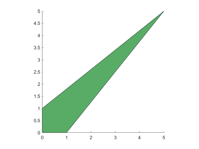
(a) Kite.

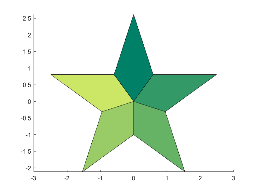
(b) Multipatch Star.

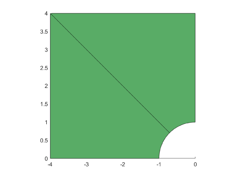
(c) Holed plate.

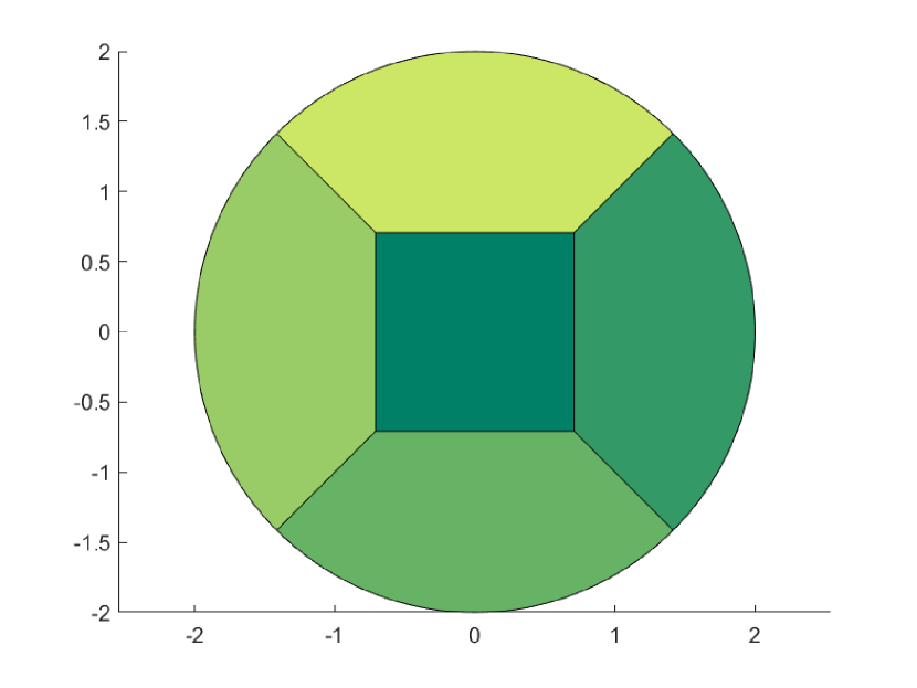
(d) Multipatch Disc.

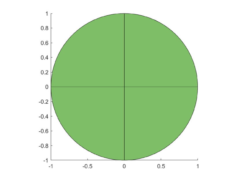
(e) Disc with one singularity.

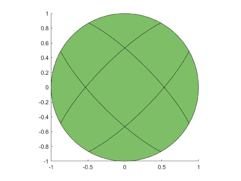
(f) Disc with four singularities.

Figure 1: Bidimensional domains.

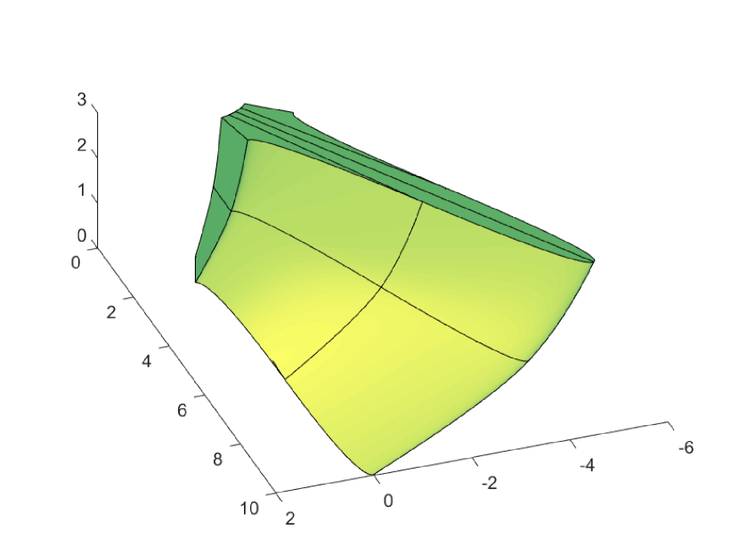
(a) Blade.

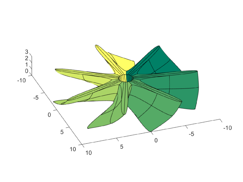
(b) Multipatch Fan.

Figure 2: Tridimensional domains.

6.1 Single Patch domains

As examples of regularly parametrized single patch domains, we consider a bidimensional kite and a tridimensional blade (see Figures 1(a) and 2(a)). For the kite domain, we compute the condition number of the unpreconditioned and preconditioned mass matrix for different values of $h$ and $p$ and report them in Tables 1 and 2, respectively. By comparing these numbers, we can see that the condition number is dramatically reduced by our preconditioning strategy. In particular, as predicted by Theorem 2, the condition number of preconditioned matrices converges to 1 as the mesh-size $h$ goes to 0. Tables 3 and 4 show the number of iterations and computation time spent by PCG for the kite and the blade domain, respectively. We emphasize that the number of iterations is always very low and even decreases when $h$ is reduced.

$n_{\mathrm{sub}}$	$p=2$	$p=3$	$p=4$	$p=5$	$p=6$
16	$5.540\cdot 10^{2}$	$2.980\cdot 10^{3}$	$1.673\cdot 10^{4}$	$9.892\cdot 10^{4}$	$6.106\cdot 10^{5}$
32	$7.040\cdot 10^{2}$	$4.063\cdot 10^{3}$	$2.435\cdot 10^{4}$	$1.523\cdot 10^{5}$	$9.853\cdot 10^{5}$
64	$8.150\cdot 10^{2}$	$4.929\cdot 10^{3}$	$3.082\cdot 10^{4}$	$2.002\cdot 10^{5}$	$1.340\cdot 10^{6}$
128	$8.900\cdot 10^{2}$	$5.536\cdot 10^{3}$	$3.555\cdot 10^{4}$	$2.366\cdot 10^{5}$	$1.617\cdot 10^{6}$

Table 1: Condition number of mass matrix for kite.

$n_{\mathrm{sub}}$	$p=2$	$p=3$	$p=4$	$p=5$	$p=6$
16	1.056	1.077	1.103	1.129	1.157
32	1.034	1.047	1.062	1.078	1.094
64	1.019	1.027	1.035	1.045	1.054
128	1.010	1.015	1.019	1.024	1.030

Table 2: Condition number of preconditioned mass matrix for kite.

$n_{\mathrm{sub}}$	$p=2$	$p=3$	$p=4$	$p=5$	$p=6$
16	4 / 0.00134	4 / 0.00141	4 / 0.00152	4 / 0.00167	4 / 0.00184
32	3 / 0.00191	3 / 0.00203	3 / 0.00225	4 / 0.00316	4 / 0.00352
64	3 / 0.00465	3 / 0.00525	3 / 0.00578	3 / 0.00675	3 / 0.00812
128	3 / 0.01550	3 / 0.01810	3 / 0.02130	3 / 0.02550	3 / 0.03100

Table 3: Iterations and time spent by PCG for kite.

$n_{\mathrm{sub}}$	$p=2$	$p=3$	$p=4$	$p=5$	$p=6$
16	6 / 0.0137	6 / 0.0315	6 / 0.0654	6 / 0.137	7 / 0.274
32	5 / 0.0821	5 / 0.1540	5 / 0.2990	5 / 0.608	6 / 1.270
64	4 / 0.4990	4 / 1.0100	4 / 1.7500	4 / 3.490	4 / 6.370

Table 4: Iterations and time spent by PCG for blade.

The case of singularly parametrized domains is beyond the theory of Section 3 (Assumption 5 does not hold). Nevertheless, we test numerically this situation on three examples: a holed plate with a singular point in the top left vertex (see Figure 1(c)); a disc with a singularity in the center (Figure 1(e)) and a disc with four singularities on the boundary (Figure 1(f)). In all the three examples the condition number is always close to 1 and, even though it does not converge to 1 as in the non-singular case, it does not grow as $h$ goes to 0. Accordingly, the number of PCG iterations is very low (see Tables 6, 8 and 10).

We are interested in studying the dependence on $p$ of the condition number of the preconditioned system. For this purpose, we follow Remark 3 and define ${\mu:=\kappa\left(\boldsymbol{\mathcal{M}}^{-\frac{1}{2}}\mathbf{M}\boldsymbol{\mathcal{M}}^{-\frac{1}{2}}\right)-1}$. For all the problems considered so far, the numerical results show that $\mu$ grows roughly linearly with respect to $p$. This phenomenon can be clearly seen in Figure 3(a). The crucial consequence of this fact is that the number of PCG iterations is almost independent of $p$. This is confirmed by the results already shown in Tables 3, 4, 6, 8 and 10.

$n_{\mathrm{sub}}$	$p=2$	$p=3$	$p=4$	$p=5$	$p=6$
16	1.692	1.861	2.018	2.173	2.330
32	1.696	1.866	2.024	2.177	2.330
64	1.699	1.869	2.028	2.182	2.334
128	1.700	1.871	2.029	2.184	2.336

Table 5: Condition number of preconditioned mass matrix for holed plate.

$n_{\mathrm{sub}}$	$p=2$	$p=3$	$p=4$	$p=5$	$p=6$
16	6 / 0.00181	7 / 0.00227	7 / 0.00248	7 / 0.00275	7 / 0.00311
32	6 / 0.00335	6 / 0.00370	6 / 0.00414	6 / 0.00466	6 / 0.00528
64	5 / 0.00734	6 / 0.00968	6 / 0.01080	6 / 0.01240	6 / 0.01510
128	5 / 0.02500	5 / 0.02870	5 / 0.03430	5 / 0.04050	5 / 0.04880

Table 6: Iterations and time spent by PCG for holed plate.

$n_{\mathrm{sub}}$	$p=2$	$p=3$	$p=4$	$p=5$	$p=6$
16	1.093	1.170	1.249	1.323	1.395
32	1.090	1.159	1.230	1.305	1.381
64	1.082	1.148	1.212	1.276	1.339
128	1.077	1.140	1.200	1.259	1.317

Table 7: Condition number of preconditioned mass matrix for disc with one singularity.

$n_{\mathrm{sub}}$	$p=2$	$p=3$	$p=4$	$p=5$	$p=6$
16	5 / 0.00156	5 / 0.00172	5 / 0.00192	6 / 0.00259	5 / 0.00259
32	4 / 0.00198	5 / 0.00274	5 / 0.00305	5 / 0.00355	5 / 0.00416
64	4 / 0.00435	4 / 0.00498	5 / 0.00693	5 / 0.00815	5 / 0.00951
128	4 / 0.01250	4 / 0.01460	4 / 0.01750	4 / 0.02200	5 / 0.03300

Table 8: Iterations and time spent by PCG for disc with one singularity.

$n_{\mathrm{sub}}$	$p=2$	$p=3$	$p=4$	$p=5$	$p=6$
16	1.167	1.252	1.350	1.459	1.575
32	1.161	1.241	1.341	1.450	1.564
64	1.158	1.237	1.338	1.447	1.559
128	1.156	1.236	1.336	1.444	1.556

Table 9: Condition number of preconditioned mass matrix for disc with four singularities.

$n_{\mathrm{sub}}$	$p=2$	$p=3$	$p=4$	$p=5$	$p=6$
16	5 / 0.00157	5 / 0.00172	6 / 0.00203	6 / 0.00229	6 / 0.00245
32	5 / 0.00282	5 / 0.00310	5 / 0.00329	5 / 0.00368	6 / 0.00478
64	4 / 0.00575	4 / 0.00648	5 / 0.00858	5 / 0.00983	5 / 0.01170
128	4 / 0.01910	4 / 0.02230	4 / 0.02640	4 / 0.03150	4 / 0.03780

Table 10: Iterations and time spent by PCG for disc with four singularities.

We now compare our preconditioner $\boldsymbol{\mathcal{M}}$ as defined in (3.5) with the preconditioner proposed by Chan and Evans in [27], that we denote by $\boldsymbol{\mathcal{M}}_{CE}$. This preconditioner has some similarity with the one we propose and, moreover, is one of the best performing to our knowledge. The application of $\boldsymbol{\mathcal{M}}_{CE}$ is, by definition, a multiplication by

$$\boldsymbol{\mathcal{M}}_{CE}^{-1}=\widehat{\mathbf{M}}^{-1}\mathbf{M}_{\det(D\boldsymbol{F})^{-1}}\widehat{\mathbf{M}}^{-1},$$

where $\mathbf{M}_{\det(D\boldsymbol{F})^{-1}}$ is a weighted mass matrix as (3.2) with $\omega=\det(D\boldsymbol{F})^{-1}$. Table 11 reports on the condition number of the preconditioned mass matrix, by $\boldsymbol{\mathcal{M}}$ and $\boldsymbol{\mathcal{M}}_{CE}$. For a more in-depth analysis of the efficiency of the two methods, we need to consider that one iteration of $\boldsymbol{\mathcal{M}}_{CE}$-PCG costs roughly as two iterations of $\boldsymbol{\mathcal{M}}$-PCG. This is because in the latter case the cost is concentrated in the matrix-vector product with $\mathbf{M}$ and the solution of a system with $\widehat{\mathbf{M}}$, while in the former case two such products (one with $\mathbf{M}$ and one with $\mathbf{M}_{\det(D\boldsymbol{F})^{-1}}$) and two such solutions are needed.

It is well-known that when Conjugate Gradient (CG) is used to solve a linear system $\mathbf{A}{x}=\mathbf{b}$, with $\mathbf{A}$ symmetric and positive definite, it holds

$$\frac{\left\|\mathbf{e}_{k}\right\|_{\mathbf{A}}}{\left\|\mathbf{e}_{0}\right\|_{\mathbf{A}}}\leq 2\left(\frac{\sqrt{\kappa\left(\mathbf{A}\right)}-1}{\sqrt{\kappa\left(\mathbf{A}\right)}+1}\right)^{k},\qquad k=1,2,\ldots,$$

where $\mathbf{e}_{k}$ is the error relative to the $k-$th iteration, and $\left\|\mathbf{e}_{k}\right\|_{\mathbf{A}}:=\sqrt{\mathbf{e}_{k}^{T}\mathbf{A}\mathbf{e}_{k}}$ for $k\geq 0$. Thus, at each iteration of CG , the upper bound on the relative error is reduced by a factor

$$q\left(\mathbf{A}\right):=\frac{\sqrt{\kappa\left(\mathbf{A}\right)}-1}{\sqrt{\kappa\left(\mathbf{A}\right)}+1}<1.$$ (6.1)

In our case, $\mathbf{A}$ is the preconditioned mass matrix. Then, we use this principle in order to compare the effectiveness of $\boldsymbol{\mathcal{M}}$ and $\boldsymbol{\mathcal{M}}_{CE}$. Since one iteration of $\boldsymbol{\mathcal{M}}_{CE}$-PCG costs twice as one iterations of $\boldsymbol{\mathcal{M}}$-PCG, we compare $q(\boldsymbol{\mathcal{M}}_{CE}^{-\frac{1}{2}}\mathbf{M}\boldsymbol{\mathcal{M}}_{CE}^{-\frac{1}{2}})$ with the factor by which the error bound is reduced after 2 iterations of $\boldsymbol{\mathcal{M}}$-PCG, which is $q(\boldsymbol{\mathcal{M}}^{-\frac{1}{2}}\mathbf{M}\boldsymbol{\mathcal{M}}^{-\frac{1}{2}})^{2}$. The results are shown in Table 12. In all cases, the bound-reducing factor is significantly small, confirming that both approaches lead to fast solvers, with an advantage for $\boldsymbol{\mathcal{M}}$ in all the considered problems and especially in the case of the singular parametrizations considered.

domain	$\kappa(\boldsymbol{\mathcal{M}}_{CE}^{-\frac{1}{2}}\mathbf{M}\boldsymbol{\mathcal{M}}_{CE}^{-\frac{1}{2}})$	$\kappa(\boldsymbol{\mathcal{M}}^{-\frac{1}{2}}\mathbf{M}\boldsymbol{\mathcal{M}}^{-\frac{1}{2}})$
kite	$1.049$	$1.157$
blade	$1.202$	$1.538$
holed plate	$1.051$	$1.216$
disc (e)	$3.652$	$1.395$
disc (f)	$3.185$	$1.575$

Table 11: Condition number of preconditioned mass matrix for $n_{\mathrm{sub}}=16$ and $p=6$: comparison between $\boldsymbol{\mathcal{M}}$ and $\boldsymbol{\mathcal{M}}_{CE}$.

domain	$q(\boldsymbol{\mathcal{M}}_{CE}^{-\frac{1}{2}}\mathbf{M}\boldsymbol{\mathcal{M}}_{CE}^{-\frac{1}{2}})$	$q(\boldsymbol{\mathcal{M}}^{-\frac{1}{2}}\mathbf{M}\boldsymbol{\mathcal{M}}^{-\frac{1}{2}})^{2}$
kite	$1.20\cdot 10^{-2}$	$1.33\cdot 10^{-3}$
blade	$4.60\cdot 10^{-2}$	$1.15\cdot 10^{-2}$
holed plate	$1.24\cdot 10^{-2}$	$2.39\cdot 10^{-3}$
disc (e)	$3.13\cdot 10^{-1}$	$6.89\cdot 10^{-3}$
disc (f)	$2.82\cdot 10^{-1}$	$1.28\cdot 10^{-2}$

Table 12: Error reduction factors relative to one iteration of $\boldsymbol{\mathcal{M}}_{CE}$-PCG (left column) and two iterations of $\boldsymbol{\mathcal{M}}$-PCG (right column), having a similar computation cost. The factors refer to the case $n_{\mathrm{sub}}=16$ and $p=6$.

6.2 Multipatch domains

Finally, in order to evaluate the performance of our Additive Schwarz preconditioner, we consider three domains: a multipatch five-pointed star (Figure 1(b)), a multipatch disc (Figure 1(d)) and a multipatch fan (Figure 2(b)), obtained by gluing together 7 blade-shaped patches like the one represented in Figure 2(a).

As in the single patch case, we compare the condition number of the original mass matrix (Tables 13 and 16) with that of the preconditioned one (Tables 14 and 17). In all cases, the preconditioner greatly reduces the condition number of the matrix, robustly with respect to $h$. Moreover, the growth of the condition number with respect to the spline degree $p$ seems to be linear (see Figure 3(b)). This is reflected also in the number of iterations needed by PCG to reach the given tolerance, see Tables 18 and 19.

$n_{\mathrm{sub}}$	$p=2$	$p=3$	$p=4$	$p=5$	$p=6$
16	$1.326\cdot 10^{2}$	$9.994\cdot 10^{2}$	$6.848\cdot 10^{3}$	$4.611\cdot 10^{4}$	$3.160\cdot 10^{5}$
32	$1.503\cdot 10^{2}$	$1.156\cdot 10^{3}$	$8.104\cdot 10^{3}$	$5.565\cdot 10^{4}$	$3.845\cdot 10^{5}$
64	$1.618\cdot 10^{2}$	$1.258\cdot 10^{3}$	$8.935\cdot 10^{3}$	$6.217\cdot 10^{4}$	$4.351\cdot 10^{5}$

Table 13: Condition number of mass matrix for multipatch star.

$n_{\mathrm{sub}}$	$p=2$	$p=3$	$p=4$	$p=5$	$p=6$
16	39.69	48.05	56.17	64.03	71.62
32	39.80	48.23	56.42	64.32	71.95
64	39.86	48.33	56.55	64.48	72.13

Table 14: Condition number of preconditioned mass matrix for multipatch star.

$n_{\mathrm{sub}}$	$p=2$	$p=3$	$p=4$	$p=5$	$p=6$
16	13 / 0.0111	14 / 0.0134	14 / 0.0145	15 / 0.0175	15 / 0.0198
32	12 / 0.0251	12 / 0.0276	13 / 0.0320	13 / 0.0375	14 / 0.0488
64	10 / 0.0647	12 / 0.0892	12 / 0.1020	12 / 0.1190	12 / 0.1410
128	09 / 0.2210	11 / 0.3030	11 / 0.3480	11 / 0.3930	12 / 0.5020

Table 15: Iterations and time spent by PCG for multipatch star.

$n_{\mathrm{sub}}$	$p=2$	$p=3$	$p=4$	$p=5$	$p=6$
16	$2.098\cdot 10^{2}$	$1.550\cdot 10^{3}$	$1.049\cdot 10^{4}$	$7.007\cdot 10^{4}$	$4.761\cdot 10^{5}$
32	$2.585\cdot 10^{2}$	$1.970\cdot 10^{3}$	$1.374\cdot 10^{4}$	$9.360\cdot 10^{4}$	$6.399\cdot 10^{5}$
64	$2.949\cdot 10^{2}$	$2.291\cdot 10^{3}$	$1.637\cdot 10^{4}$	$1.143\cdot 10^{5}$	$7.994\cdot 10^{5}$

Table 16: Condition number of mass matrix for multipatch disc.

$n_{\mathrm{sub}}$	$p=2$	$p=3$	$p=4$	$p=5$	$p=6$
16	13.88	16.02	18.03	19.92	21.70
32	13.99	16.16	18.18	20.08	21.87
64	14.06	16.24	18.28	20.18	21.98

Table 17: Condition number of preconditioned mass matrix for multipatch disc.

$n_{\mathrm{sub}}$	$p=2$	$p=3$	$p=4$	$p=5$	$p=6$
16	14 / 0.0125	15 / 0.0147	17 / 0.0180	17 / 0.0203	18 / 0.0240
32	14 / 0.0310	15 / 0.0365	16 / 0.0424	17 / 0.0513	17 / 0.0617
64	14 / 0.0995	14 / 0.1140	16 / 0.1450	16 / 0.1700	16 / 0.1960
128	14 / 0.3800	14 / 0.4210	15 / 0.4960	16 / 0.6060	16 / 0.7040

Table 18: Iterations and time spent by PCG for multipatch disc.

$n_{\mathrm{sub}}$	$p=2$	$p=3$	$p=4$	$p=5$	$p=6$
16	12 / 0.205	13 / 00.436	13 / 00.844	14 / 1.96	15 / 03.76
32	10 / 1.110	10 / 02.040	12 / 04.500	12 / 9.02	12 / 16.00
64	09 / 7.700	09 / 13.200	10 / 27.700	*	*

Table 19: Iterations and time spent by PCG for multipatch fan. In the cases denoted by “*”, we were not able to assemble the mass matrix due to memory limitations.

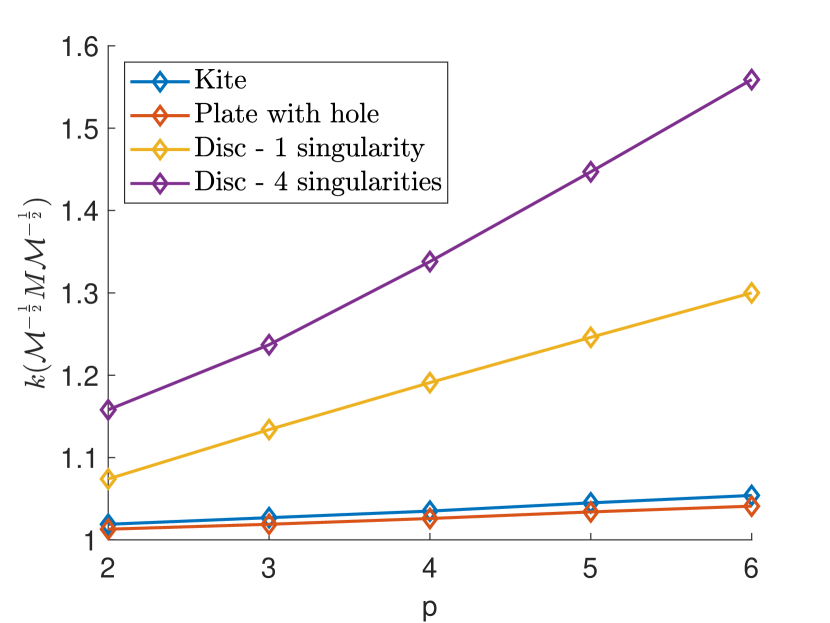
(a) Single patch domains

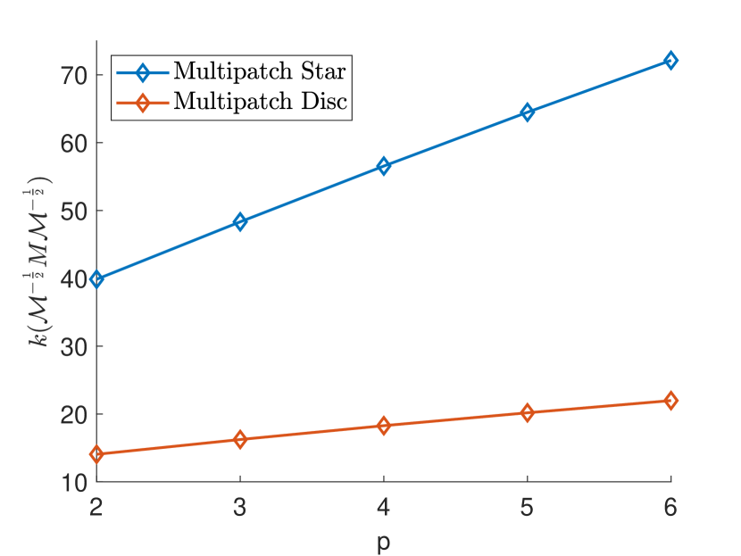
(b) Multipatch domains

Figure 3: Condition number of preconditioned mass matrix ($n_{\mathrm{sub}}=64$).

7 Conclusions

In this work, we have presented a simple and efficient preconditioner for mass matrices arising in isogeometric analysis. The main idea for the single patch case is to exploit the Kronecker product structure of parametric mass matrix on the reference domain, combined with a diagonal scaling to correctly incorporate the effect of the geometry parametrization. In order to deal with multipatch domains, we have used the single patch strategy in an Additive Schwarz preconditioner. The preconditioner has an application cost of $O(pN_{\text{dof}})$ FLOPs, and is well suited for parallelization. We have proved that the single-patch preconditioner converges, as the mesh-size $h$ goes to $0$, to the exact mass, and that robustness with respect to $h$ is preserved in the multipatch case. Numerical tests reflect the theoretical results and show a very good behaviour also with respect to the spline degree $p$.

References

• [1] T. J. R. Hughes, J. A. Cottrell, Y. Bazilevs, Isogeometric analysis: CAD, finite elements, NURBS, exact geometry and mesh refinement, Comput. Methods Appl. Mech. Engrg. 194 (39) (2005) 4135–4195.
• [2] J. A. Cottrell, T. J. R. Hughes, Y. Bazilevs, Isogeometric analysis: toward integration of CAD and FEA, John Wiley & Sons, Chichester, 2009.
• [3] Special Issue on Isogeometric Analysis: Progress and Challenges, Vol. 316 of Comput. Methods Appl. Mech. Engrg., Elsevier, 2017.
• [4] J. A. Evans, Y. Bazilevs, I. Babuška, T. J. R. Hughes, $n$-widths, sup–infs, and optimality ratios for the $k$-version of the isogeometric finite element method, Comput. Methods Appl. Mech. Engrg. 198 (21-26) (2009) 1726–1741.
• [5] L. Beirão da Veiga, A. Buffa, J. Rivas, G. Sangalli, Some estimates for $h$ $p$ $k$-refinement in isogeometric analysis, Numer. Math. 118 (2) (2011) 271–305.
• [6] E. Sande, C. Manni, H. Speleers, Sharp error estimates for spline approximation: Explicit constants, $n$-widths, and eigenfunction convergence, Math. Models Methods Appl. Sci. (2019) 1–31.
• [7] S. Takacs, T. Takacs, Approximation error estimates and inverse inequalities for B-splines of maximum smoothness, Math. Models Methods Appl. Sci. 26 (07) (2016) 1411–1445.
• [8] A. Bressan, E. Sande, Approximation in FEM, DG and IGA: A theoretical comparison, arXiv preprint arXiv:1808.04163.
• [9] G. Sangalli, M. Tani, Matrix-free weighted quadrature for a computationally efficient isogeometric $k$-method, Comput. Methods Appl. Mech. Engrg. 338 (2018) 117–133.
• [10] S. Hartmann, D. Benson, A. Nagy, Isogeometric analysis with LS-DYNA, Journal of Physics: Conference Series 734 (2016) 032125.
• [11] A. Bünger, S. Dolgov, M. Stoll, A low-rank tensor method for pde-constrained optimization with isogeometric analysis, SIAM Journal on Scientific Computing 42 (1) (2020) A140–A161.
• [12] C. Hofreither, W. Zulehner, Mass smoothers in geometric multigrid for isogeometric analysis, in: International Conference on Curves and Surfaces, Springer, Cham, 2014, pp. 272–279.
• [13] C. Hofreither, S. Takacs, Robust multigrid for isogeometric analysis based on stable splittings of spline spaces, SIAM J. Numer. Anal. 55 (4) (2017) 2004–2024.
• [14] H. C. Elman, D. J. Silvester, A. J. Wathen, Finite elements and fast iterative solvers: with applications in incompressible fluid dynamics, Oxford University Press, USA, 2014.
• [15] T. Elguedj, Y. Bazilevs, V. M. Calo, T. J. R. Hughes, B and F projection methods for nearly incompressible linear and non-linear elasticity and plasticity using higher-order NURBS elements, Comput. Methods Appl. Mech. Engrg. 197 (33-40) (2008) 2732–2762.
• [16] E. Brivadis, A. Buffa, B. Wohlmuth, L. Wunderlich, Isogeometric mortar methods, Comput. Methods Appl. Mech. Engrg. 284 (2015) 292–319.
• [17] M. Łoś, M. Paszyński, A. Kłusek, W. Dzwinel, Application of fast isogeometric L2 projection solver for tumor growth simulations, Comput. Methods Appl. Mech. Engrg. 316 (2017) 1257–1269.
• [18] J. Evans, R. Hiemstra, T. J. R. Hughes, A. Reali, Explicit higher-order accurate isogeometric collocation methods for structural dynamics, Comput. Methods Appl. Mech. Engrg. 338 (2018) 208–240.
• [19] F. Auricchio, L. Beirão da Veiga, T. J. R. Hughes, A. Reali, G. Sangalli, Isogeometric collocation for elastostatics and explicit dynamics, Comput. Methods Appl. Mech. Engrg. 249-252 (2012) 2–14.
• [20] A. Tkachuk, M. Bischoff, Direct and sparse construction of consistent inverse mass matrices: general variational formulation and application to selective mass scaling, Internat. J. Numer. Methods Engrg. 101 (6) (2015) 435–469.
• [21] L. Wunderlich, A. Seitz, M. D. Alaydın, B. Wohlmuth, A. Popp, Biorthogonal splines for optimal weak patch-coupling in isogeometric analysis with applications to finite deformation elasticity, Comput. Methods Appl. Mech. Engrg. 346 (2019) 197–215.
• [22] L. Gao, V. M. Calo, Fast isogeometric solvers for explicit dynamics, Comput. Methods Appl. Mech. Engrg. 274 (2014) 19–41.
• [23] M. Woźniak, M. Łoś, M. Paszyński, L. Dalcin, V. M. Calo, Parallel fast isogeometric solvers for explicit dynamics, Comput. Inform. 36 (2) (2017) 423–448.
• [24] A. Mantzaflaris, B. Jüttler, B. N. Khoromskij, U. Langer, Matrix generation in isogeometric analysis by low rank tensor approximation, in: International Conference on Curves and Surfaces, Springer, Cham, 2014, pp. 321–340.
• [25] A. Mantzaflaris, B. Jüttler, B. N. Khoromskij, U. Langer, Low rank tensor methods in galerkin-based isogeometric analysis, Comput. Methods Appl. Mech. Engrg. 316 (2017) 1062–1085.
• [26] C. Hofreither, A black-box low-rank approximation algorithm for fast matrix assembly in isogeometric analysis, Comput. Methods Appl. Mech. Engrg. 333 (2018) 311–330.
• [27] J. Chan, J. A. Evans, Multi-patch discontinuous Galerkin isogeometric analysis for wave propagation: Explicit time-stepping and efficient mass matrix inversion, Comput. Methods Appl. Mech. Engrg. 333 (2018) 22–54.
• [28] C. De Boor, A practical guide to splines, Revised Edition, Vol. 27 of Applied Mathematical Sciences, Springer-Verlag, New York, 2001.
• [29] L. Schumaker, Spline Functions: Basic Theory, 3rd Edition, Cambridge Mathematical Library, Cambridge University Press, Cambridge, 2007.
• [30] L. Beirão da Veiga, A. Buffa, G. Sangalli, R. H. Vázquez, Mathematical analysis of variational isogeometric methods, Acta Numer. 23 (2014) 157––287.
• [31] T. G. Kolda, B. W. Bader, Tensor decompositions and applications, SIAM Rev. 51 (3) (2009) 455–500.
• [32] C. De Boor, Splines as linear combinations of b-splines a survey, in: Approximation Theory, II, Academic Press, New York, 1976, pp. 1–47.
• [33] A. Toselli, O. Widlund, Domain decomposition methods—algorithms and theory, Vol. 34 of Springer Series in Computational Mathematics, Springer-Verlag, Berlin, 2005.
• [34] L. Beirão da Veiga, D. Cho, L. F. Pavarino, S. Scacchi, Overlapping Schwarz methods for isogeometric analysis, SIAM J. Numer. Anal. 50 (3) (2012) 1394–1416.
• [35] R. H. Vázquez, A new design for the implementation of isogeometric analysis in Octave and Matlab: GeoPDEs 3.0, Comput. Math. Appl. 72 (3) (2016) 523–554.