Statistical Mechanics of Confined Polymer Networks

Abstract

We show how the theory of the critical behaviour of $d$-dimensional polymer networks of arbitrary topology can be generalized to the case of networks confined by hyperplanes. This in particular encompasses the case of a single polymer chain in a bridge configuration. We further define multi-bridge networks, where several vertices are in local bridge configurations. We consider all cases of ordinary, mixed and special surface transitions, and polymer chains made of self-avoiding walks, or of mutually-avoiding walks, or at the tricritical $\Theta$-point. In the $\Theta$-point case, generalising the good-solvent case, we relate the critical exponent for simple bridges, $\gamma_{b}^{\Theta}$, to that of terminally-attached arches, $\gamma_{11}^{\Theta},$ and to the correlation length exponent $\nu^{\Theta}.$ We find $\gamma_{b}^{\Theta}=\gamma_{11}^{\Theta}+\nu^{\Theta}.$ In the case of the special transition, we find $\gamma_{b}^{\Theta}({\rm sp})=\frac{1}{2}[\gamma_{11}^{\Theta}({\rm sp})+\gamma_{11}^{\Theta}]+\nu^{\Theta}.$ For general networks, the explicit expression of configurational exponents then naturally involve bulk and surface exponents for multiple random paths. In two-dimensions, we describe their Euclidean exponents from a unified perspective, using Schramm-Loewner Evolution (SLE) in Liouville quantum gravity (LQG), and the so-called KPZ relation between Euclidean and LQG scaling dimensions. This is done in the case of ordinary, mixed and special surface transitions, and of the $\Theta$-point. We provide compelling numerical evidence for some of these results both in two- and three-dimensions.

Keywords: Polymer networks, confinement, bridges, surface transitions, self-avoiding walks, mutually-avoiding random walks, tricritical $\Theta$-point, conformal invariance, Schramm-Loewner Evolution, Liouville quantum gravity, KPZ relation.

In celebration of the achievements of our dear colleague Joel L. Lebowitz.

1 Introduction

1.1 A brief history

Long polymer chains in a good solvent can be modelled in the continuum by the celebrated Edwards model [81], or, in a discrete setting, as self-avoiding walks (SAWs) on a lattice. It is well-known that they constitute a critical system. This was originally recognized in a breakthrough paper by P.-G. de Gennes [88] (which was part of his 1991 Nobel Prize in Physics) through their equivalence to a magnetic $n$-component spin model, with $O(n)$ symmetry, in the limit $n\to 0$. This allowed him to obtain the size and configuration critical exponents $\nu$ and $\gamma$ of a single polymer chain, such that for $N\to+\infty$,

$$R^{2}\propto N^{2\nu},$$ (1)

$$\mathcal{Z}\propto{\mu}^{N}N^{\gamma-1},$$ (2)

where $R^{2}$ is the averaged square end-to-end distance of a chain of $N$ monomers, and $\mathcal{Z}$ its partition function in a continuum model, or its self-avoiding configuration number in the lattice setting (up to translations) [85, 91]. The constant $\mu$ is the connective constant, or growth constant which is model-dependent, and whose existence was established by Hammersley in the lattice case [96]. In the magnetic $n$-component model, $\nu$ and $\mu$ are the universal correlation length and susceptibility exponents, which depend solely on $n$ and the space dimension $d$. Scaling expressions such as (1) and (2) are expected to hold up to fixed but non-universal amplitude factors. The $\varepsilon$-expansions of $\nu,\gamma$ in space dimension $d=4-\varepsilon$ were then obtained in the famous Wilson-Fisher renormalization group approach [146] to the $(\varphi^{2})^{2}$ interacting theory of a $n$-component field $\varphi$, taken in the $n\to 0$ limit in the polymer case [88]. This original field theoretic approach was successfully extended to the case of polymer solutions by J. des Cloizeaux [27] (see also [129, 130, 147]), who later invented a direct renormalization method [28, 29, 30] for the canonical Edwards model, which had the great advantage of being both geometrically intuitive and efficient, and was shown to be equivalent to that of field theory [15, 48]. The so-called Flory $\Theta$-point, where the solvent quality suddenly decreases [85], corresponds to a tricritical phase transition [89] and to a $(\varphi^{2})^{3}$ interacting theory of a $n$-component field $\varphi$, still in the $n\to 0$ limit [90, 46]. (For a recent mathematical study, see [10, 11]). The corresponding canonical Edwards model with 3-body interactions is itself amenable to a direct renormalization method [47, 15, 49, 30]. Extensive Neutron and Light scattering experiments were performed on polymer solutions in the 70’s, which neatly confirmed scaling and renormalization theories [24, 25]. Comprehensive monographs are [30, 127].

In the case of two-dimensional self-avoiding walks, a breakthrough occurred in 1982, when B. Nienhuis [116, 117] (see also [21]) used a mapping of the $O(n)$ model on the hexagonal lattice to a Coulomb gas to predict the exact (albeit non-rigorous) values of the critical exponents,

$$\nu=3/4,\quad\gamma=43/32.$$ (3)

Another unexpected approach came in 1988 from so-called two-dimensional quantum gravity when Knizhnik, Polyakov and Zamolodchikov discovered the celebrated KPZ relation between critical exponents in the plane and those on a random lattice [100, 32, 39], via the use of Liouville quantum gravity (LQG) [121]. It allowed in particular another derivation of SAW’s exponents (3) from a direct computation on a random lattice [66, 67].

Finally, one should mention the groundbreaking invention in 1999 of Stochastic Loewner Evolution (SLE) by Oded Schramm [131], which was a game-changer for the mathematical approach to the two-dimensional statistical mechanics of critical phenomena. It has already resulted in the attribution of two Fields Medals, in 2006 to Wendelin Werner for his work with Greg Lawler and Oded Schramm on Brownian intersection exponents [106, 107, 108] and the Mandelbrot conjecture [109], and in 2010 to Stanislav Smirnov for his proof of the convergence on the hexagonal lattice of site percolation interfaces to SLE₆ [136], and Ising model interfaces to SLE₃ [137, 22]. Interestingly, while planar self-avoiding walks are strongly expected to converge in the continuum to SLE_8/3 [110], a proof has so far eluded even the best mathematical minds. Notice, however, that Nienhuis’ 1982 famous prediction that the SAW connective constant equals $\mu=\sqrt{2+\sqrt{2}}$ on the hexagonal lattice was proven 30 years later [45]! (See also [12] for the corresponding SAW critical adsorption fugacity $1+\sqrt{2}$).

1.2 Higher polymer topologies

1.2.1 Stars.

Outside the usual linear chain case, other polymer topologies are possible, the most natural one being that of a star $\mathcal{S}_{L}$, made up of $L$ self- and mutually avoiding arms of similar or equal lengths $N$. While the typical size of a star still scales like $N^{\nu}$, the star partition function or number of configurations (up to translations) now behaves for $N\to+\infty$ as,

$$\mathcal{Z}\left({\mathcal{S}_{L}}\right)\propto{\mu}^{LN}N^{\gamma_{\mathcal{S}_{L}}-1},$$ (4)

where $\mu$ is the same connective constant as in the linear chain case (2) [145], whereas $\gamma_{\mathcal{S}_{L}}$ is a critical exponent characteristic of the star topology, directly linked to the presence of an $L$-leg vertex. The single-chain case corresponds to $L=1$, and $\gamma_{\mathcal{S}_{1}}=\gamma$. For $L=2$, one has a two-leg star which is still a single linear polymer, hence $\gamma_{\mathcal{S}_{2}}=\gamma$. For $L\geq 3$, the $\gamma_{\mathcal{S}_{L}}$’s constitute a new set of independent critical exponents. In two-dimensions for instance, their values were predicted via conformal invariance methods and Coulomb-gas methods [50, 124] to be

$$\gamma_{\mathcal{S}_{L}}-1=\frac{1}{64}\big{(}4+9L(3-L)\big{)},$$ (5)

in good agreement with the numerical results of exact enumeration and Monte-Calo techniques [111, 145]. For $L=1,2$, one recovers $\gamma$ as in (3).

Another illustrative example is that of a uniform star at the $\Theta$-point in three dimensions, which is the upper-tricritical dimension, where only logarithmic corrections to Brownian or random walk behavior occur. Its partition function can be shown via a direct renormalization of the relevant Edwards model to scale as [52],

$$\mathcal{Z}^{\Theta}\left({\mathcal{S}_{L}}\right)\propto{\mu_{\Theta}}^{LN}(\log N)^{-\frac{1}{22}{{L}\choose{3}}},$$

where $\mu_{\Theta}$ is the (model-dependent) connective constant at the $\Theta$-point, and where the log-power is expected to be universal.

Beyond that of stars and combs [87, 111, 145], the most general case of self-avoiding or $\Theta$-point polymer networks of arbitrary but fixed topologies was considered in any dimension via an extensive treatment of their configurational critical exponents, and published thirty years ago in the same Journal of Statistical Physics [55]. It elaborated on the results of earlier Letters, the first one covering the bulk case in a good solvent [50], motivated by the results of [124] in two-dimensions, and followed by extensions to networks at the ordinary surface transition, or at the $\Theta$-point [71, 72, 52]. The present article can be seen as a distant-in-time sequel to these works (see also [118]).

1.2.2 Boundaries and bridges.

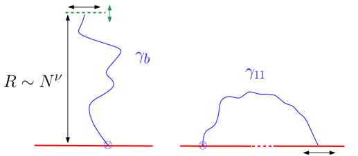
Figure 1: A polymer chain of length $N$ anchored at a surface, in bridge configurations below an hyperplane, with entropic exponent $\gamma_{b}$ (left), and in surface arch configurations with entropic exponent $\gamma_{11}$ (right). In each case, and to eliminate overall translational invariance, one (and only one) vertex ($\otimes$) is fixed along the surface. Compared to the motion of the second surface vertex in the arch configuration, the top-most vertex of the bridge configuration is free to move along a further direction perpendicular to the surface, by distances of order $R\sim N^{\nu}$, resulting in the simple scaling law $\gamma_{b}=\gamma_{11}+\nu$.

We recently revisited this theory to show that it can be extended to describe the statistics of self-avoiding walks in bridge or worm configurations [65]. As a result, the bridge configurational exponent was shown to equal

$$\gamma_{b}=\gamma_{11}+\nu,$$ (6)

where $\gamma_{11}$ is the usual configurational arch surface exponent at the ordinary surface transition corresponding to Dirichlet boundary conditions. The simple geometrical argument for this identity is recalled in Fig. 1. In the presence of increasingly attractive surface interactions, a special surface phase transition may occur, where the chain contracts towards the surface, just before collapsing onto it. At this special transition point, the bridge exponent is

$$\gamma_{b}({\rm sp})=\frac{1}{2}\left[\gamma_{11}({\rm sp})+\gamma_{11}\right]+\nu,$$ (7)

where $\gamma_{11}({\rm sp})$ is now the special transition arch surface exponent [65]. The worm configurational exponent was found to obey $\gamma=\gamma_{w}+\nu$, where $\gamma$ is the usual entropic exponent of a bulk SAW. The shift by $\nu$ here, as well as in Eqs. 6 and 7, is brought about by the same mechanism as that described in Fig. 1. These results were based on the general theory yielding the configurational critical exponents associated with polymer networks of any topology, to which we now turn.

1.2.3 General configurational exponents.

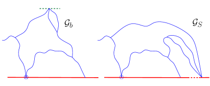
Figure 2: Polymer networks interacting with a surface. To eliminate overall translational invariance, one (and only one) vertex ($\otimes$) is fixed along the surface. Both networks have $\mathcal{N}=8$ lines, with respective lengths all scaling like $N$, with $N\to\infty$. Both networks possess 4 bulk vertices, of which $n_{1}=1$ has one line, and $n_{3}=3$ have three lines attached. Network ${\mathcal{G}}_{S}$ on the right has 3 surface vertices, $n_{1}^{S}=1$ with one leg, $n_{2}^{S}=1$ with two legs, and $n_{3}^{S}=1$ with three legs. Network ${\mathcal{G}}_{b}$ on the left is in a bridge configuration. It has the same surface vertices, except for the 3-leg surface vertex being replaced by the (top-most) 3-leg bridge vertex.

Consider surface-attached polymer networks such as those represented in Fig. 2. One arbitrary boundary vertex is fixed to eliminate overall translations. The partition function or number of configurations of such a self-avoiding (monodisperse) $d$-dimensional polymer network ${\mathcal{G}_{S}}$, made of $\mathcal{N}$ chains of equal lengths $N$, is given for $N\to+\infty$ by an expression similar to (2) and (4),

$${\mathcal{Z}}\left({\mathcal{G}_{S}}\right)\propto{\mu}^{\mathcal{N}N}N^{\gamma_{\mathcal{G}_{S}}-1},$$ (8)

with the same the growth constant $\mu$ as in the single chain case. The configurational critical exponent $\gamma_{\mathcal{G}_{S}}$ is given by the explicit exact formula [50, 71, 55, 118],

$$\gamma_{\mathcal{G}_{S}}=\nu\left[d{\mathcal{V}}+(d-1)({\mathcal{V}}_{S}-1)-\sum_{L\geq 1}(n_{L}x_{L}+n_{L}^{S}x_{L}^{S})\right]-({\mathcal{N}}-1).$$ (9)

Here ${\mathcal{V}}$ is the number of bulk vertices, ${\mathcal{V}}_{S}$ is the number of surface vertices, $n_{L}$ is the number of $L$-leg vertices floating in the bulk, while $n_{L}^{S}$ is the number of $L$-leg vertices on or constrained close to, the surface. ${\mathcal{N}}$ denotes the number of chains in the network. The intuitive meaning of formula (9) for such a configurational exponent $\gamma_{\mathcal{G}_{S}}$ is clear: the first two terms correspond, via the correlation lengh exponent $\nu$, to the Euclidean phase space of the (bulk and surface) vertices of the network, the $x_{L}$ and $x_{L}^{S}$ (universal) critical exponents correspond to the entropic reduction in phase space induced by both linkage and self- or mutual-avoidance in each $L$-star vertex, and the last term, $\mathcal{N}-1$, corresponds to the constraint of monodispersity in the $\mathcal{N}$ arms of the network (i.e., their respective lengths, or monomer numbers, all scale like $N$, with $N\to+\infty$).

For an unconstrained network $\mathcal{G}$ in the bulk, with no surface attached vertices, $d{\mathcal{V}}$ must be replaced by $d({\mathcal{V}}-1),$ as otherwise one is counting all translates, and the formula simply becomes [50, 55]

$$\gamma_{\mathcal{G}}=\nu\left[d({\mathcal{V}}-1)-\sum_{L\geq 1}n_{L}x_{L}\right]-({\mathcal{N}}-1).$$ (10)

For an illustrative example, let us return to the star bulk case $\mathcal{G}:=\mathcal{S}_{L}$, for which $\mathcal{V}=L+1$, $\mathcal{N}=L$, $n_{1}=L$, and $n_{L}=1$. Eq. (10) then gives

$$\gamma_{\mathcal{\mathcal{missing}}S_{L}}=\nu(Ld-Lx_{1}-x_{L})-(L-1).$$

For $L=1,2$, we have

$$\gamma_{\mathcal{S}_{1}}=\nu(d-2x_{1});\quad\gamma_{\mathcal{S}_{2}}=\nu(2d-2x_{1}-x_{2})-1.$$ (11)

Since $\gamma_{\mathcal{S}_{1}}=\gamma_{\mathcal{S}_{2}}=\gamma$, we have $\nu(d-x_{2})=1$, hence the known identity $x_{2}=d-1/\nu$ [117, 55].

A non-trivial result, of course, is that such a reduction in (9) or (10) to individual vertices holds true; it can be obtained in 2 dimensions from conformal field theory [50, 71, 55], or from a two-dimensional quantum gravity approach [66, 67]. In generic dimension $d$, one resorts to the multiplicative renormalization theory of polymer networks [55, 128], which is an extension of that of polymer chains [28, 29, 30, 127].

The values of the universal critical exponents $\nu$, $x_{L}$ and $x^{S}_{L}$ naturally all depend on the space dimension and on the universality class of the polymer problem considered: SAWs, polymer chains at the $\Theta$-point, or mutually-avoiding random walks, and, concerning the surface case, ordinary or special transition boundary conditions. All these values will be made precise below. One of the aims of this work is to present these exponents in the two-dimensional case, often initially derived in theoretical physics from Coulomb gas, conformal invariance or Bethe Ansatz methods, from a more unified perspective, and in particular to place them in broader families of critical exponents, that can be derived within the recent SLE and Liouville Quantum Gravity mathematical frameworks [61, 69, 78].

Note that the simplest case where the multiplicative renormalization theory presented above can be established in a straightforward way is that of Brownian networks made up of simple random walks, or, in the continuum, Brownian chains. In this case, the scaling exponent $\nu=1/2$, and the bulk and Dirichlet surface $L$-leg exponents are (see, e.g., [53])

$$x^{\rm B}_{L}=\frac{L}{2}(d-2),\,\,\,\,x^{S,{\rm B}}_{L}=\frac{L}{2}d.$$ (12)

Note their proportionality to $L$, coming from the statistical independence of Brownian paths. In this case, formulae (9) and (10) can be reduced to simpler expressions, using the topological identities for the total chain number $\mathcal{N}$, independent loop number $\mathscr{L}$, and bulk and surface vertex numbers $\mathcal{V}$ and ${\mathcal{V}}_{S}$,

$$\mathcal{N} = \frac{1}{2}\sum_{L\geq 1}L(n_{L}+n_{L}^{S}),\,\,\,\,\mathscr{L}=\frac{1}{2}\sum_{L\geq 1}(L-2)(n_{L}+n_{L}^{S})+1,$$ (13)

$$\mathcal{V} = \sum_{L\geq 1}n_{L},\,\,\,\,{\mathcal{V}}_{S}=\sum_{L\geq 1}n_{L}^{S}.$$ (14)

For a pure bulk Brownian network, this together with (12) gives for Eq. (10)

$$\gamma^{\rm B}_{\mathcal{G}}-1=-{\mathscr{L}}d/2,$$ (15)

a well-known result in the computation of polymer Feynman diagrams (see, e.g., [53, 55]). When the Brownian network is attached onto a Dirichlet surface, one finds for (9) [55, Section 6]

$$\gamma^{\rm B}_{\mathcal{G}_{S}}-1=-{\mathscr{L}}d/2-\frac{1}{2}({\mathcal{V}}_{S}-1)-\frac{1}{2}{\mathcal{L}}_{S},$$ (16)

where ${\mathcal{L}}_{S}:=\sum_{L\geq 1}Ln_{L}^{S}$ is the number of chains terminally touching the surface.

2 Polymer networks and bridges

2.1 Bridges

A bridge configuration $\mathcal{G}_{b}$ in a polymer network anchored to a surface appear when a given $L$-leg vertex is the top-most point of the network (Fig. 2, left). This constraint is equivalent to the appearance of a movable virtual top-most hyperplane, contributing in Eq. (9) a boundary exponent $x_{L}^{S}$, as in the right-most polymer network $\mathcal{G}_{S}$ in Fig. 2 that results from the topological move as represented in Fig. 3. However, because the virtual top-most hyperplane is movable, the said top-most $L$-vertex in $\mathcal{G}_{b}$ contributes one unit to the number ${\mathcal{V}}$ of bulk vertices in Eq. (9), whereas the boundary vertex in $\mathcal{G}_{S}$ contributes one unit to the number ${\mathcal{V}}_{S}$ of boundary vertices in Eq. (9). We thus have in all generality for the pair of networks in Figs. 2, 3,

$$\gamma_{\mathcal{G}_{b}}=\gamma_{\mathcal{G}_{S}}+\nu,$$ (17)

which yields a direct generalisation of identity (7).

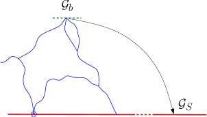
Figure 3: Transformation of the bridge polymer network ${\mathcal{G}}_{b}$ into a surface network ${\mathcal{G}}_{S}$ in Fig. 2. The single extra spatial degree of freedom of the movable hyperplane of the (3-leg) bridge vertex with respect to the corresponding (3-leg) surface vertex induces the simple scaling relation of the respective configuration exponents, $\gamma_{{\mathcal{G}}_{b}}=\gamma_{{\mathcal{G}}_{S}}+\nu$.

2.2 Multi-bridges

Figure 4: A multi-bridge polymer network ${\mathcal{G}}_{b}$ anchored at a surface. To eliminate overall translational invariance, one (and only one) vertex ($\otimes$) is fixed along the surface. This network has $n_{1}^{b}=1$ single bridge vertex and $n_{3}^{b}=1$ 3-leg bridge vertex, where the polymer strands are locally confined below their respective hyperplanes (e.g., up to the next connected vertices). The lengths of the $\mathcal{N}=11$ chains of the network all scale like $N$, with $N\to\infty$.

The bridge theory presented so far can be extended to multi-bridge network configurations. These are defined only locally: a given $L$-vertex is said to be an $L$-multi-bridge if each of the $L$ chains attached to it stay below (or above) the vertex at least up to the second vertex to which it is bound. An example is given in Fig. 4. Such a multi-bridge vertex contributes a term $-\nu x_{L}^{S}$, together with a free-volume term $+\nu d$, to the entropic exponent $\gamma_{\mathcal{G}}$. Denoting by $n_{L}^{b}$ the numbers of $L$-bridge vertices, we therefore arrive at a more general form of the entropic exponent of a multi-bridge network $\mathcal{G}_{b}$,

$$\gamma_{\mathcal{G}_{b}}=\nu\left[d{\mathcal{V}}+(d-1)({\mathcal{V}}_{S}-1)-\sum_{L\geq 1}\big{(}n_{L}x_{L}+(n_{L}^{S}+n_{L}^{b})x_{L}^{S}\big{)}\right]-({\mathcal{N}}-1),$$ (18)

where now the bulk and surface vertex numbers are, respectively,

$${\mathcal{V}}=\sum_{L\geq 1}(n_{L}+n_{L}^{b}),\,\,\,\,\,\,{\mathcal{V}}_{S}=\sum_{L\geq 1}n_{L}^{S}.$$ (19)

2.3 Special transition

If there is an attractive surface fugacity $a=\exp(-\epsilon/k_{B}T),$ where $\epsilon$ is the energy associated with a monomer of the walk lying in the surface, then this has no effect on the critical point or critical exponent of the network provided that $a$ is less than its critical value $a_{c}>1,$ where $a_{c}$ is called the critical fugacity. Precisely at the critical fugacity, the exponent changes discontinuously. This is called the special transition, and the corresponding expression to Eq. (9) follows straightforwardly by replacing the Dirichlet scaling dimensions $x_{L}^{S}$ by their values at the special transition, $x_{L}^{S}({\rm sp})$. This extension to the case of polymer networks at the special transition in two-dimensions was given in [4], who also included the mixed case of some surface vertices being at the critical fugacity and others not. In this mixed case, the general formula (9), as well as the multi-bridge one (18) obviously generalize to

$$\gamma_{\mathcal{G}_{S}}=\nu\left[d{\mathcal{V}}+(d-1)({\mathcal{V}}_{S}-1)-\sum_{L\geq 1}\big{(}n_{L}x_{L}+n_{L}^{S}x_{L}^{S}+n_{L}^{S}({\rm sp})x_{L}^{S}({\rm sp})\big{)}\right]-({\mathcal{N}}-1),$$ (20)

$$\gamma_{\mathcal{G}_{b}}=\nu\left[d{\mathcal{V}}+(d-1)({\mathcal{V}}_{S}-1)-\sum_{L\geq 1}\big{(}n_{L}x_{L}+(n_{L}^{S}+n_{L}^{b})x_{L}^{S}+n_{L}^{S}({\rm sp})x_{L}^{S}({\rm sp})\big{)}\right]-({\mathcal{N}}-1),$$ (21)

where $n_{L}^{S}({\rm sp})$ represents the number of surface $L$-leg vertices at the special transition point, and where now $\mathcal{V}=\sum_{L\geq 1}\left(n_{L}+n_{L}^{b}\right)$ and $\mathcal{V}_{S}=\sum_{L\geq 1}\left(n_{L}^{S}+n_{L}^{S}({\rm sp})\right)$.

For $a>a_{c}$ the location of the critical point varies monotonically with $a,$ and the exponents change to integers, corresponding to poles in the generating function. In this paper we will only consider the situation $a\leq a_{c},$ which corresponds to the most interesting physics.

2.4 A consistency check

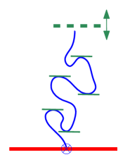
Figure 5: Consistency check of the scaling theory of local bridges: Any local extremum along an anchored polymer chain (which may be part of a larger network $\mathcal{G}_{S}$), can be seen as a virtual two-leg bridge vertex, yielding a reduced-entropy contribution $-\nu x_{2}^{S}=-\nu d$ to $\gamma_{\mathcal{G}}$ in Eq. (9), together with a volume contribution $+\nu d$ due to its bulk degrees of freedom, in effect yielding no overall contribution. The same is true in $\Theta$-point conditions where $x_{2}^{S,\Theta}=d$ also holds.

A peculiar case in the network-multibridge theory presented here is that of local extremal points along the chains making up the network (Fig. 5). Even though they fleetingly appear in the configuration space, they can be considered as genuine two-leg vertices associated with a local bridge point (i.e., a local top-most or bottom-most point). Each then should contribute a $-\nu x_{2}^{S}$ Dirichlet surface term, together with a usual volume term $+\nu d$ to configuration exponent $\gamma_{\mathcal{G}_{S}}$ (10). However, it is a fundamental fact [55, Section 6.5.1] (see also [38]) that in any dimension $d$, the two-leg ordinary transition surface exponent for a polymer chain with excluded volume takes its Brownian or random walk value (12)

$$x_{2}^{S}=x_{2}^{S,\mathrm{B}}=d.$$ (22)

This also holds for polymer chains at the $\Theta$-point, as we shall see below. Thus, the two contributions exactly cancel, and extremal points along a chain yield no contribution to the entropy of the chain, as it must. Note that this argument can be reversed to yield the simplest proof that one necessarily has, for Dirichlet ordinary boundary conditions, the 2-leg surface exponent $x_{2}^{S}\equiv d$, irrespective of the universality class of the polymer chain (SAW, $\Theta$-point, Brownian).

3 Multiple-path critical exponents

In this section, we first briefly recall the values of bulk exponents $x_{L}$, surface exponents $x_{L}^{S}$, and special surface exponents $x_{L}^{S}(\mathrm{sp})$, as well as some generalisations of them. In a second step, in the two-dimensional case, we provide a direct, general technique [61, 69] to compute them with the help of Liouville quantum gravity (LQG) and of the famous Knizhnik-Polyakov-Zamolodchikov (KPZ) relation [100], adapted to the Schramm-Loewner Evolution (SLE) [131]. This will in particular be useful in the case of polymer networks at the $\Theta$-point in two-dimensions. This approach is naturally related to multiple SLE theory [9, 14, 44, 92, 101, 102, 103, 148, 149] (For a recent mathematical perspective, see [119, 120].)

3.1 A short survey

In two-dimensions, the bulk conformal weights $(\frac{1}{2})x_{L},$ and surface conformal weights $x_{L}^{S},$ associated with $L-$vertices, are explicitly given by

$$x_{L}=\frac{1}{48}(3L-2)(3L+2),\,\,\,\,\,\,x_{L}^{S}=\frac{1}{8}L(3L+2),$$ (23)

with $1/\nu=2-x_{2}=4/3$. (See Refs. [116, 117] for the $L=1,2$ bulk cases, Ref. [20] for the $L=1$ boundary case, and [124, 125, 66, 5, 61] for the general bulk case, and [71, 93, 17, 18, 6, 82, 61] for the general boundary case). In $d$-dimensions, they have the general form [55],

$$x_{L}=x^{\rm B}_{L}+x^{\prime}_{L},\,\,\,\,\,\,x^{S}_{L}=x^{S,{\rm B}}_{L}+x^{\prime S}_{L},$$

where the first terms are the Brownian scaling dimensions (12), whereas the second ones, $x^{\prime}_{L},\,x^{\prime S}_{L}$, represent the anomalous contributions from self- and mutual avoidance. At first orders in $\varepsilon:=4-d$, the latter are [30, 55]

$$x^{\prime}_{L}=\frac{\varepsilon}{8}L(L-1)+\left(\frac{\varepsilon}{8}\right)^{2}\frac{L}{4}\left(-8L^{2}+33L-23\right)+O(\varepsilon^{3}),$$

and

$$x^{\prime S}_{L}=\frac{\varepsilon}{8}L(L-2)+O(\varepsilon^{2}),$$ (24)

while being also explicitly known to next order in $\varepsilon$ [33, 34, 35, 82, 84, 128]. For $d\geq 4$, $x^{\prime}_{L}=0,x^{\prime S}_{L}=0$, with known logarithmic corrections to Brownian network partition functions at $d=4$ [55].

As we have seen, Eqs. (9), (10), and (18) naturally hold in the case of random walks or Brownian chains, for which $\nu=1/2$ and the scaling exponents take the above mentioned Brownian values (12). They also hold in the mixed case of a network made of mutually-avoiding (M) random walks or Brownian chains, for which the bulk and surface scaling exponents are in two-dimensions [68, 56, 106, 107]

$$x_{L}^{\rm M}=\frac{1}{12}(4L^{2}-1),\,\,\,x_{L}^{\rm M,S}=\frac{1}{3}L(2L+1).$$ (25)

In $d=4-\varepsilon$ dimensions the bulk exponent is [53]

$$x_{L}^{\rm M}=x_{L}^{\rm B}+\frac{\varepsilon}{4}L(L-1)-\left(\frac{\varepsilon}{4}\right)^{2}L(L-1)(2L-5)+O(\varepsilon^{3}),$$

while for $d\geq 4$, $x_{L}^{\rm{M}}=x_{L}^{\rm B}$ and $x_{L}^{\rm M,S}=x_{L}^{S,\rm B}$, with known logarithmic corrections at $d=4$ [53].

Notice that for SAWs, as announced in Section 2.4, the 2-leg Dirichlet surface exponent in two-dimensions is from (23) $x_{2}^{S}=2=d=x_{2}^{S,\mathrm{B}}$, i.e., the Brownian one, in agreement with Eq. (22), and that in $d$-dimensions, the anomalous addition $x^{\prime S}_{L}$ (24) to the Brownian surface exponent vanishes for $L=2$ at first-order (as it does to all orders).

At the special transition point, the scaling dimensions $x_{L}^{S}$ (23) are replaced by their values in two-dimensions, obtained in Refs. [83, 7, 8, 150] (see [93] for the $L=1$ case and see also [17, 18, 54]),

$$x_{L}^{S}({\rm sp})=\frac{3}{8}L^{2}-\frac{3}{4}L+\frac{1}{3}.$$ (26)

3.2 LQG-KPZ derivation of 2D exponents

3.2.1 Introduction.

In [61, 62], a systematic way is provided to compute critical exponents of SLE (i.e., of the $O(n)$ or Potts models in two-dimensions), by extensively using a technique imported from Liouville quantum gravity. It consists in calculating similar “quantum” exponents as measured with the LQG random measure (which represents the random area measure generated in a 2D critical random lattice). Then, Euclidean critical exponents, as defined with respect to the usual Lebesgue measure in the plane, are expressed in a unique way in terms of the former quantum ones via the celebrated KPZ relation [100, 32, 39]. The interest of the method is that some quantum exponents can be calculated using random matrix theory (RMT), as was originally done in the late ’80s [99, 66, 67]. Furthermore, as shown in [135, 69], they enjoy fundamental conformal welding properties (by “cutting and gluing”), which make their computation remarkably simple, and this without recourse to RMT nor Coulomb gas methods. The KPZ relation has been mathematically proven in various settings in the last decade [77, 78, 123, 70, 63, 3], and, as we shall se below, the quantum gravity techniques advocated here [59, 60, 61, 62] are part and parcel of the conformal welding of so-called quantum wedges and cones, introduced in the recent mathematical theory of Liouville quantum gravity as developed in [69] (see also [64, 95] for introductions).

The Schramm-Loewner Evolution, SLE_κ, is a canonical conformally invariant process in the plane, either in the disk $\mathbb{D}$ (called radial), or in the half-plane $\mathbb{H}$ (called chordal) or in the whole-plane $\mathbb{C}$. It crucially depends on a single real parameter $\kappa\geq 0$. For $0\leq\kappa\leq 4$, the random paths generated are simple, whereas for $4<\kappa<\infty$ they continually self-intersect (but do not self-cross). For $\kappa\geq 8$, they are Peano curves in the plane. The relation to the critical $O(n),n\in[0,2]$, model in the plane is given by $n=-2\cos\left(4\pi/\kappa\right)$, with $\kappa\in[8/3,4]$ for the dilute critical point, and $\kappa\in[4,8]$ for the so-called dense phase of the $O(n)$-model [60, 61, 98]. For the Potts critical model with parameter $Q\in[0,4]$, there is complete equivalence to the universality class of the $O(n)$ dense phase, via the simple identity $n=\sqrt{Q}$ [116, 117, 51].

3.2.2 KPZ relation and duality.

In Refs. [61, Section 11.1] and [62, Section 10.2], the following KPZ formulae, adapted to computations with SLE_κ, were proposed,

$$\mathcal{U}_{\kappa}(\Delta) = \frac{1}{4}\Delta\left(\kappa\Delta+4-\kappa\right),$$ (27)

$$\mathcal{V}_{\kappa}(\Delta) = \mathcal{U}_{\kappa}\left[\frac{1}{2}\left(\Delta+1-\frac{4}{\kappa}\right)\right]=\frac{1}{16\kappa}\left[\kappa^{2}\Delta^{2}-(4-\kappa)^{2}\right].$$ (28)

Function $\mathcal{U}_{\kappa}$ transforms SLE_κ quantum boundary scaling exponents $\Delta$ into their Euclidean boundary counterparts, $x^{S}=\mathcal{U}_{\kappa}(\Delta)$, whereas function $\mathcal{V}_{\kappa}$ transforms these into their Euclidean bulk counterparts, $x=2\mathcal{V}_{\kappa}(\Delta)$ [61, 62]. As explained in detail there, these were precisely devised to be insensitive to the usual change of parameterization of Liouville quantum gravity between the $\kappa\in[0,4]$ and $\kappa\in(4,\infty)$ ranges. Actually, for $\kappa\in[0,4]$, Eqs. (27) is the usual KPZ relation [78] $U_{\gamma}(\Delta)=\frac{1}{4}\Delta\left(\gamma^{2}\Delta+4-\gamma^{2}\right)$, where $\gamma=\sqrt{\kappa}\in[0,2]$ is the Liouville measure parameter. When $\kappa\in(4,\infty)$, it is the dual KPZ relation [61, 62, 63, 3, 64] $U_{4/\gamma}(\Delta)$, where $\gamma=\sqrt{16/\kappa}\in(0,2)$.

3.2.3 Multiple SLE exponents.

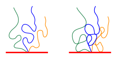
Figure 6: $L=3$ multiple chordal SLE_κ paths rooted at a surface in two-dimensions. Left: For $\kappa\leq 4$, the paths are simple and do not touch each other, nor the surface outside of the root. Right: For $\kappa>4$, the chains are non-simple, bounce repeatedly onto each other and onto the surface.

In the case of multiple SLE_κ paths originating at a boundary point in $\mathbb{H}$ (Fig 6), the quantum boundary exponent $\Delta$ is built by simply adding the individual contributions $2/\kappa$ of each path separately [61, 62], namely,

$$\Delta=\Delta_{L}^{\kappa}:=2L/\kappa.$$ (29)

Note that for $\kappa\leq 4$, $\Delta_{L}^{\kappa}$ is a usual (additive) quantum boundary exponent in LQG, whereas for $\kappa>4$, it represents the dual quantum boundary exponent that is additive. (See [61, Section 12.1] and [62, Section 10.5].) This leads to [61, 62, 148, 149]

$$x^{S,\kappa}_{L}=\mathcal{U}_{\kappa}(\Delta_{L}^{\kappa}) = \frac{L}{2\kappa}\left(2L+4-\kappa\right),$$ (30)

$$x_{L}^{\kappa}=2\mathcal{V}_{\kappa}(\Delta_{L}^{\kappa}) = \frac{1}{8\kappa}\left[4L^{2}-(4-\kappa)^{2}\right].$$ (31)

One must then recall that the boundary behaviour of chordal SLE_κ strongly depends on its phase (Fig. 6): If $\kappa\leq 4$, the random paths do not intersect the boundary line. If $\kappa>4$, the SLE_κ paths continually touch and bounce onto the boundary. Nevertheless, (30) corresponds in both cases to the ordinary boundary phase for the corresponding $O(n)$-model.

3.2.4 Conditioning boundary intersections ($\kappa>4$).

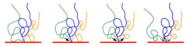
Figure 7: $L=3$ multiple chordal SLE_κ>4 paths in two-dimensions. For $\kappa>4$, they continually bounce onto themselves and onto each other. The paths can be conditioned in several ways. Left: Ordinary boundary conditions where the paths repeatedly bounce onto the surface, with surface exponent $x_{L=3}^{S,\kappa}=x_{L=3,j=0}^{S,\kappa}$. Middle left: Mixed boundary conditions (as marked by one arrow) where the leftmost path is conditioned not to hit the surface outside the root, with exponent $x_{L=3,j=1}^{S,\kappa}$. Middle right: The leftmost and rightmost paths are conditioned not to intersect the boundary, as marked by two arrows, with exponent $x_{L=3,j=2}^{S,\kappa}$. Right: Three non-intersection conditions are imposed, resulting in exponent $x_{L=3,j=3}^{S,\kappa}$. Each arrow indicates the addition of a unit of quantum dimension (33) in (34).

Let us introduce the positive inverse of function $\mathcal{U}_{\kappa}$ (27),

$$\mathcal{U}^{-1}_{\kappa}(x)=\frac{1}{2\kappa}\left(\sqrt{16\kappa x+(4-\kappa)^{2}}+\kappa-4\right).$$ (32)

As shown in [61, Section 12.1], and [62, Section 10.5], for $\kappa>4$, thus for non-simple SLE_κ>4 paths, one can condition the paths constituting an SLE_κ $L$-star not to intersect the boundary, by inserting along the boundary ‘point operators’ with a non-vanishing quantum scaling dimension,

$$\mathcal{U}^{-1}_{\kappa}(0)=\vartheta(\kappa-4)\left(1-4/\kappa\right),$$ (33)

where $\vartheta(x)=0,x<0;\vartheta(0)=1/2;\vartheta(x)=1,x>0$, is the Heaviside distribution. For a total number $j\in\{0,1,2\}$ of such insertions, one obtains the first three boundary conditional cases depicted in Fig 7. This operation can also be performed between any two paths, which, by conformal invariance, acts in the same way as an insertion in between the left-most path (or the right-most path) and the boundary (Fig. 7, right-most case with $j=3$). Thus, one can take $0\leq j\leq L+1$ for the boundary case, and $0\leq j\leq L$ for the bulk case.

For $\kappa>4$, dual quantum boundary dimensions are additive in LQG (See [61, Section 12.1] and [62, Section 10.5].) This leads us to define a new (dual) quantum boundary exponent,

$$\Delta^{\kappa}_{L,j}:=\Delta_{L}^{\kappa}+j\,\mathcal{U}^{-1}_{\kappa}(0)=\frac{2L}{\kappa}+j\,\vartheta(\kappa-4)\left(1-\frac{4}{\kappa}\right),$$ (34)

associated with a boundary-attached $L$-star, with a number $j$ of arm-splittings.

These dual quantum boundary dimensions now are the seeds to generate Euclidean boundary and bulk scaling exponents via the (dual) KPZ relation (27),

$$x^{S,\kappa}_{L,j}:=\mathcal{U}_{\kappa}(\Delta^{\kappa}_{L,j}) = \frac{1}{4}\Delta^{\kappa}_{L,j}\left(\kappa\Delta^{\kappa}_{L,j}+4-\kappa\right)=\frac{\kappa}{4}\Delta^{\kappa}_{L,j}\Delta^{\kappa}_{L,j-1},$$

$$0\leq j\leq L+1,$$

$$x^{\kappa}_{L,j}:=2\mathcal{V}_{\kappa}(\Delta^{\kappa}_{L,j}) = 2\,\mathcal{U}_{\kappa}\left[\frac{1}{2}\left(\Delta^{\kappa}_{L,j}+1-\frac{4}{\kappa}\right)\right]=2\,\mathcal{U}_{\kappa}\left[\frac{1}{2}\Delta^{\kappa}_{L,j+1}\right]$$ (36)

$$= \frac{\kappa}{8}\Delta^{\kappa}_{L,j+1}\Delta^{\kappa}_{L,j-1},\,\,\,0\leq j\leq L.$$

This gives for $\kappa>4$ the set of explicit Euclidean exponents,

$$x^{S,\kappa}_{L,j} = \frac{\kappa}{4}\Delta^{\kappa}_{L,j}\Delta^{\kappa}_{L,j-1},\,\,\,\,\,\,0\leq j\leq L+1,$$ (37)

$$= \frac{1}{4\kappa}\left[{2L}+j\,\left({\kappa}-{4}\right)\right]\left[{2L}+(j-1)\,\left({\kappa}-{4}\right)\right],$$

$$x^{\kappa}_{L,j} = \frac{\kappa}{8}\Delta^{\kappa}_{L,j+1}\Delta^{\kappa}_{L,j-1},\,\,\,\,\,\,0\leq j\leq L,$$ (38)

$$= \frac{1}{8\kappa}\left[{2L}+(j+1)\,\left(\kappa-{4}\right)\right]\left[{2L}+(j-1)\,\left(\kappa-{4}\right)\right].$$

These exponents describe for $\kappa>4$ an $L$-star SLE_κ with $j$ constraints associated with the conditioning of non-intersection of $j$ pairs of paths or pairs comprised of a path and a boundary line, either in the chordal setting with $0\leq j\leq L+1$, or in the radial or whole-plane setting with $0\leq j\leq L$ [61, 62]. The $j=0,1$ cases of exponents (37) appear in [149], and the $j=0,1,2$ cases of exponents (38) in [148].

For $j=0$, we recover exponents (30), (31), which together with the $j=1$ and $j=2$ cases yield the boundary exponents,

$$x^{S,\kappa}_{L,j=0} = \frac{L}{2\kappa}\left({2L}+4-{\kappa}\right),$$ (39)

$$x^{S,\kappa}_{L,j=1} = \frac{L}{2\kappa}\left({2L}+{\kappa}-{4}\right),$$ (40)

$$x^{S,\kappa}_{L,j=2} = \frac{1}{2\kappa}\left({L}+{\kappa}-{4}\right)\left({2L}+{\kappa}-{4}\right).$$ (41)

These exponents will be used later in application to polymers at the $\Theta$-point in two-dimensions.

3.2.5 Duality and path frontiers.

It is known that the external frontier of a non-simple SLE${}_{\kappa^{\prime}}$ process $\eta^{\prime}$ with $\kappa^{\prime}>4$ is a form of simple SLE_κ process $\eta$ with dual parameter $16/\kappa^{\prime}=:\kappa<4$ [59, 61, 43, 151]. For instance, one has for their respective Hausdorff dimensions $\mathrm{dim}_{H}(\eta^{\prime})=2-x_{2}^{\kappa^{\prime}}=1+\kappa^{\prime}/8$, and $\mathrm{dim}_{H}(\eta)=1+2/\kappa^{\prime}=2-x_{2}^{\kappa}=1+\kappa/8$. Near an ordinary boundary, a similar duality holds. Indeed, for $L=2$, Eqs. (39) and (41) yield the identity

$$x^{S,\kappa^{\prime}}_{L=2,j=2}=\frac{1}{2}\left({\kappa^{\prime}}-{2}\right)=\frac{1}{\kappa}\left(8-{\kappa}\right)=x^{S,\kappa}_{L=2,j=0}.$$ (42)

This means that a non-simple path $\eta^{\prime}$, anchored at a surface and conditioned not to hit it outside the boundary root, is conformally equivalent to the simple path $\eta$ made by its external frontier anchored at the same root.

3.3 Conformal welding of quantum wedges

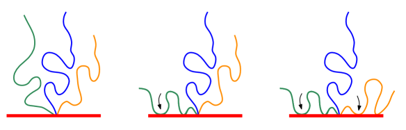
Figure 8: $L=3$ multiple chordal SLE_κ≤4 paths in two-dimensions. For $\kappa\leq 4$, the simple paths do not touch each other, nor the surface. The paths can be conditioned in various ways. Left: Ordinary boundary conditions where the paths avoid the surface, with exponent $x_{L}^{S,\kappa}$. Middle: Conditioning one path (as marked by one arrow) to intersect the surface. Right: Conditioning two paths (as marked by arrows) to intersect the surface.

3.3.1 Introduction.

In this section, we shall make use of the formalism of conformal welding of quantum wedges and cones in Liouville Quantum Gravity (LQG), as developed in Refs. [135] and [69]. We shall first use it to condition multiple SLE_κ paths for $\kappa\leq 4$, and further show how to recover and interpret the scaling dimensions (37) and (38) for $\kappa>4$ in that formalism.

We shall need the SLE${}_{\kappa}(\rho)$ process [143, 144, 43], an important variant of the standard $\mathrm{SLE}_{\kappa}$ process. In its chordal version in $\mathbb{H}$, it has a special point marked near the origin on $\partial\mathbb{H}$ ($0^{+}$, say), and roughly speaking, the parameter $\rho$ indicates whether there is an attraction ($\rho<0$) to, or a repulsion ($\rho>0$) from the half-boundary $\mathbb{R}^{+}$. When $\rho<\kappa/2-2\leq 0$, the corresponding curves will touch the boundary; when $\rho>\kappa/2-2$, the curves do not touch the boundary except at the end points, as depicted in Fig. 8. This description of the boundary behaviour of cordal SLE${}_{\kappa}(\rho)$ (with a force point located at $0^{+}$) can be read off from the almost sure Hausdorff dimension of the intersection of its trace $\eta$ with the rightmost part of the boundary. For $\rho\in(-2\vee\kappa/2-4,\kappa/2-2)$, it is [40, 41, 115, 142],

$$\textrm{dim}(\eta\cap\mathbb{R}^{+})=1-\beta,\,\,\,\beta=\beta(\rho):=\frac{1}{\kappa}(2+\rho)(2+\rho+2-\kappa/2),$$ (43)

such that $0<\textrm{dim}(\eta\cap\mathbb{R}^{+})<1$ for $\rho\in(-2\vee\kappa/2-4,\kappa/2-2)$. For $\rho>\kappa/2-2$, the trace does not intersect the boundary. Similarly, one can define a chordal $\textrm{SLE}_{\kappa}(\rho_{1},\rho_{2})$ process with two force points located at $0^{-}$ and $0^{+}$.

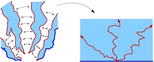
Figure 9: Four quantum wedges conformally welded along boundaries according to their boundary quantum length, and conformally mapped to $\mathbb{H}$. The images of the interfaces are coupled SLE${}_{\kappa}(\rho_{1},\rho_{2})$ processes.

3.3.2 Simple SLE paths ($\kappa\leq 4$).

Consider Fig. 8. Here, we view it as depicting a collection of chordal SLE_κ≤4 paths $\eta_{i}$, $1\leq i\leq L$. For $2\leq i\leq L-1$, the conditional law of each path $\eta_{i}$, given $\eta_{j}$ for $j\neq i,$ is that of an SLE_κ in the component of $\mathbb{H}\setminus\cup_{j\neq i}\eta_{j}$ between $\eta_{i-1}$ and $\eta_{i+1}$, whereas the conditional law of $\eta_{i=1}$ is that of an SLE${}_{\kappa}(\rho_{1})$ in the sector between $\mathbb{R}^{-}$ and $\eta_{2}$, and the conditional law of $\eta_{i=L}$ is that of an SLE${}_{\kappa}(\rho_{2})$ in the sector between $\eta_{L-1}$ and $\mathbb{R}^{+}$. The marginal law of $\eta_{i}$ for each $i=1,\cdots,L$ is that of an SLE${}_{\kappa}(\rho_{1}+2(i-1),2(L-i)+\rho_{2})$ process. This setting is a slight generalisation of that considered for $\rho_{1}=\rho_{2}=0$ in [69, Appendix B.4, Figure B.2]. We shall in the sequel use the terminology and results of Ref. [69]; for smoother introductions, see [64, 95].

As shown in Fig. 9, and explained in [69, Appendix B.4], this collection of SLE_κ paths can be obtained by first considering in LQG a so-called quantum wedge $\mathcal{W}$, made by gluing together $L+1$ independent quantum wedges $\mathcal{W}_{i},i=1,\cdots,L+1$, of respective weights $W_{1}=2+\rho_{1}$, $W_{i}=2,i=2,\cdots L$, and $W_{L+1}=2+\rho_{2}$.The conformal welding of these independent wedges is made according to their $\gamma$-LQG boundary length, followed by a conformal mapping to $\mathbb{H}$. The resulting $L$ interfaces are then represented by the set $\eta_{i},i=1,\cdots,L,$ of SLE_κ curves. The LQG parameter $\gamma$ which determines the quantum boundary measure $e^{\gamma h/2}dx$ [77, 78], where $h$ is an instance of the Gaussian Free Field (GFF) with free boundary conditions, is related to $\kappa$ by the fundamental relation [135, 79, 69],

$$\gamma=\sqrt{\kappa}\wedge\frac{4}{\sqrt{\kappa}}.$$ (44)

In term of this Liouville parameter $\gamma$, the standard KPZ relation is [77, 78, 63, 64]

$$x=U_{\gamma}(\Delta):=\frac{\gamma^{2}}{4}\Delta^{2}+\left(1-\frac{\gamma^{2}}{4}\right)\Delta,$$ (45)

$$\Delta=U^{-1}_{\gamma}(x)=\frac{1}{\gamma}\left[\sqrt{4x+a^{2}_{\gamma}}-a_{\gamma}\right],\,\,\,a_{\gamma}:=\frac{2}{\gamma}-\frac{\gamma}{2},$$ (46)

and is identical to Eq. (27) in the case $\kappa\leq 4$, where $\gamma^{2}=\kappa$. This is in particular the case we are dealing with in this section.

The weight of the wedge $\mathcal{W}$ resulting from the welding of independent wedges is simply the sum of their individual weights,

$$W=\sum_{i=1}^{L+1}W_{i}=2(L+1)+\rho_{1}+\rho_{2}.$$ (47)

According to the LQG formalism (see [69, Section 1.1 and Appendix B]), such a wedge $\mathcal{W}$ of weight $W$ is an $\alpha$-quantum wedge where

$$\alpha=\gamma+2/\gamma-W/\gamma,$$ (48)

such that the Gaussian free field $h$ is locally $\alpha$-thick (corresponding to a singularity $-\alpha\log|\cdot|$ at the origin). As explained in [78, Eq. (63)] and in [79], a “quantum typical” point in a random fractal of quantum scaling exponent $\Delta$ is then a point near which the field is $\alpha$-thick, with

$$\alpha=\gamma(1-\Delta).$$ (49)

This in turn yields the simple wedge-boundary scaling exponent relation [69],

$$W=2+\gamma^{2}\Delta.$$ (50)

Here the quantum typical point is the origin of the $L$-multiple SLE curves, the marked point of quantum wedge $\mathcal{W}$ of weight $W$ (47). It has for quantum boundary scaling exponent $\Delta=\Delta_{L}^{\kappa}(\rho_{1},\rho_{2})$, where

$$\Delta_{L}^{\kappa}(\rho_{1},\rho_{2}):=\frac{1}{\gamma^{2}}(W-2)=\frac{2L}{\kappa}+\frac{1}{\kappa}(\rho_{1}+\rho_{2}),$$ (51)

where use was made of $\gamma^{2}=\kappa$ from Eq. (44) for $\kappa\leq 4$. By using the KPZ relation (27), we therefore get the set of Euclidean boundary conformal weights,

$$x_{L}^{S,\kappa}(\rho_{1},\rho_{2}):=\mathcal{U}_{\kappa}(\Delta_{L}^{\kappa}(\rho_{1},\rho_{2}))=\frac{1}{4\kappa}(2L+\rho_{1}+\rho_{2})(2L+\rho_{1}+\rho_{2}+4-\kappa),$$ (52)

which correspond to the boundary scaling behaviour of the set of $L$-multiple chordal SLE_κ paths $\eta_{i},i=1,\cdots,L$ (Figs. 8 and 9). As already shown in [69, Appendix B.6], we recover for $L=2,\rho_{1}=\rho_{2}=\rho$, the scaling exponent $x_{2}^{S,\kappa}(\rho,\rho)=\beta(\rho)$ that gives the Hausdorff dimension (43) of the boundary intersection of SLE${}_{\kappa}(\rho)$.

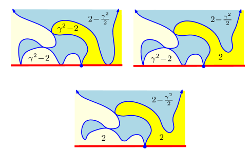
Figure 10: Boundary cases for $L=1$ and $j\in\{0,1,2\}$ in Section 3.3.3: A quantum wedge $\mathcal{W}_{1}$ of weight $W_{1}=2-\gamma^{2}/2$ (in blue) is associated with the region surrounded by a non-simple SLE_κ>4 path $\eta_{1}$, whose left and right boundaries are represented as thick lines with arrows (in dark blue). Wedges ${\widetilde{\mathcal{W}}}_{\ell=1,2}$ (in light or bright yellow) have weights $\widetilde{W}_{\ell=1,2}$ equal to either $\gamma^{2}-2$ or $2$ depending on whether $\eta_{1}$ is unconditioned or conditioned not to intersect the corresponding half-boundary, respectively.

3.3.3 Non-simple SLE paths near a boundary ($\kappa>4$).

Consider again Fig. 7, and the collection it depicts of SLE_κ>4 non-simple paths $\eta_{i},i=1,\cdots,L$, in clockwise order, and with the further convention that $\eta_{0}=\mathbb{R}^{-}$ and $\eta_{L+1}=\mathbb{R}^{+}$. Here, following [69, Appendices B.2, B.4, B.5] we view their configuration in $\mathbb{H}$ as resulting from the conformal welding of a set of $2L+1$ independent quantum wedges, followed by a conformal map to $\mathbb{H}$ (Fig. 10). These wedges are of two main types. Wedges $\mathcal{W}_{i},i=1,\cdots,L,$ represent the regions surrounded by the non-simple paths $\eta_{i},i=1,\cdots,L$, i.e., the wedges located in between the left and right boundary of each path $\eta_{i}$. Each of them has weight $W_{i}=2-\gamma^{2}/2$ [69]. They are separated from the boundary and from each other by another set of wedges $\widetilde{\mathcal{W}}_{\ell},\ell=1,\cdots L+1$, interspersed in between wedges $\mathcal{W}_{i},i=1,\cdots,L$. The wedge $\widetilde{\mathcal{W}}_{\ell=i}$ represents the quantum space in between the right boundary of $\eta_{i}$ and the left boundary of $\eta_{i+1}$. If the latter two are free to be in contact, the weight of $\widetilde{\mathcal{W}}_{i}$ is ${\widetilde{W}}_{i}=\gamma^{2}-2$, whereas if $\eta_{i}$ and $\eta_{i+1}$ are conditioned not to hit each other, the weight is ${\widetilde{W}}_{i}=2$ [69, Appendix 4]. Equivalently, the conditional law of $\eta_{i}$ is that of an SLE${}_{\kappa}(\kappa-4)$ if it is simply conditioned not to intersect $\eta_{i-1}$, and that of an SLE${}_{\kappa}(\kappa-4,\kappa-4)$ if it does not intersect both $\eta_{i-1}$ and $\eta_{i+1}$ [43, 114]. Let us now assume that there is a number $j$, $0\leq j\leq L+1,$ of such conditionings. In Fig. 7, these conditionings are represented by arrows located in between SLE paths, while in Fig. 10, they correspond to the presence of wedges of weight $2$.

The resulting wedge $\mathcal{W}$ has for its weight the sum of individual weights,

$$W = L(2-\gamma^{2}/2)+(L+1-j)(\gamma^{2}-2)+2j$$

$$= L\gamma^{2}/2+(4-\gamma^{2})j+\gamma^{2}-2.$$

The relation (50) between a quantum wedge weight $W$ and the corresponding boundary quantum scaling exponent $\Delta$ yields for the weight (3.3.3) a boundary quantum scaling exponent $\Delta=\Delta_{L,j}$,

$$\Delta_{L,j} := \frac{1}{\gamma^{2}}(W-2)=\frac{L}{2}+(j-1)\left(\frac{4}{\gamma^{2}}-1\right).$$ (54)

Recall that exponents $\Delta^{\kappa}_{L,j}$ in Eq. (34) are for $\kappa>4$ dual quantum dimensions. By definition [61, 62, 63], the dual $\widetilde{\Delta}$ of a quantum scaling exponent $\Delta$ obeys

$$\gamma(1-\Delta)=(4/\gamma)(1-\widetilde{\Delta}).$$ (55)

The relation (50) between a quantum wedge weight $W$ and the corresponding boundary quantum scaling exponent $\Delta$ thus becomes for its dual $\widetilde{\Delta}$ [64, Appendix B.3],

$$W=\gamma^{2}-2+4\widetilde{\Delta}.$$ (56)

Therefore, the weight (3.3.3) yields a dual boundary quantum scaling exponent $\widetilde{\Delta}=\widetilde{\Delta}_{L,j}$, where

$$\widetilde{\Delta}_{L,j} := \frac{1}{4}(W+2-\gamma^{2})=\frac{\gamma^{2}}{8}L+j\left(1-\frac{\gamma^{2}}{4}\right).$$ (57)

Using now (44) for $\kappa>4$ gives $\gamma^{2}=16/\kappa$, and we get the pair of dual boundary quantum scaling dimensions,

$$\Delta_{L,j} = \frac{L}{2}+(j-1)\left(\frac{\kappa}{4}-1\right),$$ (58)

$$\widetilde{\Delta}_{L,j} = \frac{2L}{\kappa}+j\left(1-\frac{4}{\kappa}\right)=\Delta^{\kappa}_{L,j},$$ (59)

where, as expected, Eq. (59) coincides with Eq. (34) for the dual quantum dimension.

Finally, using either the standard KPZ relation (45) for the standard quantum dimension (58), or equivalently, its dual version (27) for the dual dimension (59), we get

$$x^{S,\kappa}_{L,j}=U_{\gamma}\left(\Delta_{L,j}\right)=\mathcal{U}_{\kappa}\left(\Delta^{\kappa}_{L,j}\right)=\frac{1}{4\kappa}\left[{2L}+j\,\left({\kappa}-{4}\right)\right]\left[{2L}+(j-1)\,\left({\kappa}-{4}\right)\right],$$ (60)

which coincides with Eq. (37).

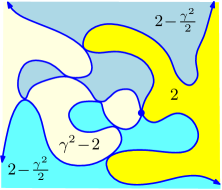
Figure 11: Bulk case for $L=2$ and $j=1$ in Section 3.3.4: Two quantum wedges $\mathcal{W}_{i=1,2}$ of weight $W_{i=1,2}=2-\gamma^{2}/2$ (in blue and cyan) are associated with the regions surrounded by two non-simple SLE_κ>4 paths $\eta_{i=1,2}$, whose left and right boundaries are represented as thick lines with arrows (in dark blue). Wedge ${\widetilde{\mathcal{W}}}_{1}$ (in light yellow) has weight $\widetilde{W}_{1}=\gamma^{2}-2$ because the left boundary of $\eta_{1}$ and the right boundary of $\eta_{2}$ are allowed to intersect, while wedge ${\widetilde{\mathcal{W}}}_{2}$ (in bright yellow) has weight $\widetilde{W}_{2}=2$ because the right boundary of $\eta_{1}$ and the left boundary of $\eta_{2}$ are conditioned not to intersect.

3.3.4 Non-simple SLE paths in the bulk ($\kappa>4$).

Consider the local behaviour of a collection of $L$ successive whole-plane SLE_κ>4 processes $\eta_{i}$, $i=1,\cdots,L,$ near a quantum typical multiple point $z_{0}$ of order $L$, with a number $j$, $0\leq j\leq L$, of conditionings of pairs of successive, non-intersecting paths. It can be represented by gluing together $2L$ independent wedges of alternating weights $2-\gamma^{2}/2$, for the region surrounded by each $\eta_{i}$, and either $2$ or $\gamma^{2}-2$ for the region between $\eta_{i}$ and $\eta_{i+1}$, depending on whether the pair $(\eta_{i},\eta_{i+1})$ is conditioned not to intersect or is not conditioned (Fig 11; see also [69, Appendix B.5] in the $j=0$ case). This yields a total weight,

$$W=L\left(2-\frac{\gamma^{2}}{2}\right)+2j+\left(L-j\right)\left(\gamma^{2}-2\right)=L\frac{\gamma^{2}}{2}+j(4-\gamma^{2}).$$ (61)

By the conformal welding theory in Liouville quantum gravity [69, Proposition (7.16)], gluing together these $2L$ wedges yields a so-called $\alpha$-quantum cone associated with a local singularity $-\alpha\log|\cdot-z_{0}|$ near the $L$-multiple point $z_{0}$, where

$$\alpha:=Q-\frac{W}{2\gamma},\,\,\,Q:=\frac{\gamma}{2}+\frac{2}{\gamma}.$$

Its explicit value is here,

$$\alpha=\frac{2}{\gamma}+\frac{\gamma}{2}-\frac{\gamma}{4}L-\left(\frac{2}{\gamma}-\frac{\gamma}{2}\right)j.$$ (62)

Finally, let $\Delta=\Delta^{\circ}_{L,j}$ be the bulk quantum dimension associated with this $\alpha$-cone so that $\alpha=\gamma(1-\Delta)$. We find

$$\Delta^{\circ}_{L,j}=\frac{L}{4}+\frac{1}{2}(j-1)\left(\frac{4}{\gamma^{2}}-1\right).$$ (63)

Because of Definition (55), the dual dimension $\widetilde{\Delta}$ of $\Delta$ obeys $\alpha=(4/\gamma)(1-\widetilde{\Delta})$, so that the dual of dimension (63) reads with the help of (62),

$$\widetilde{\Delta}^{\circ}_{L,j}=1-\frac{\gamma}{4}\alpha=\left(\frac{\gamma}{4}\right)^{2}L+\frac{1}{2}(j+1)\left(1-\frac{\gamma^{2}}{4}\right).$$ (64)

These results hold for $\kappa>4$ and $\gamma^{2}=16/\kappa$. We thus arrive at the pair of dual bulk quantum dimensions,

$$\Delta^{\circ}_{L,j} = \frac{L}{4}+\frac{1}{2}(j-1)\left(\frac{\kappa}{4}-1\right),$$ (65)

$$\widetilde{\Delta}^{\circ}_{L,j} = \frac{L}{\kappa}+\frac{1}{2}(j+1)\left(1-\frac{4}{\kappa}\right)=:\Delta^{\circ\,\kappa}_{L,j},$$ (66)

where we used the dual version to define $\Delta^{\circ\,\kappa}_{L,j}$ in (66), in accordance with the definition of the dual dimension $\Delta^{\kappa}_{L,j}$ in Eq. (59). We thus have the relationship between the quantum boundary and bulk dimensions (58) and (65), or between their respective duals (59) and (66),

$$\Delta_{L,j} =2\Delta^{\circ}_{L,j},$$ (67)

$$\Delta^{\kappa}_{L,j}= \widetilde{\Delta}_{L,j} =2\widetilde{\Delta}^{\circ}_{L,j}-(1-\gamma^{2}/4)=2\Delta^{\circ\,\kappa}_{L,j}-(1-4/\kappa),$$ (68)

in full agreement with previous results for the dense phase of the $O(n)$ model and for SLE_κ>4 non-simple paths. (See [61, Section 10.3, Equations (10.23) and (10.24); Section 11.1, Equation (11.2)].)

Finally, using either the standard KPZ relation (45) for the standard bulk quantum dimension (63) or (65), or equivalently, its dual versions (27) and (28) for the dual dimensions (66) and (59), we get the corresponding set of bulk Euclidean scaling dimensions,

$$x^{\kappa}_{L,j} = 2U_{\gamma}\left(\Delta^{\circ}_{L,j}\right)=2\,\mathcal{U}_{\kappa}\left(\Delta^{\circ\,\kappa}_{L,j}\right)=\mathcal{V}_{\kappa}\left(\Delta^{\kappa}_{L,j}\right)$$ (69)

$$= \frac{1}{8\kappa}\left[{2L}+(j+1)\,\left({\kappa}-{4}\right)\right]\left[{2L}+(j-1)\,\left({\kappa}-{4}\right)\right],$$

which coincides with Eq. (38), as expected.

3.4 Special boundary conditions

In this section, we shall recast results known for the special surface transition of the $O(n)$ model at its dilute critical point, in terms of the formalism of multiple SLE${}_{\kappa}(\rho_{1},\rho_{2})$ paths, as described in Section 3.3.2 above. For the special surface transition the boundary $L$-star exponents $x_{L}^{S}(\textrm{sp})$ are given by [83, 7, 8, 150]

$$x_{L}^{S}(\textrm{sp})=\frac{1}{4}g(L+1)^{2}-\frac{3}{2}(L+1)+\frac{1}{4g}[9-(g-1)^{2}],$$ (70)

with $g$ the Coulomb gas coupling constant such that $n=-2\cos\pi g$, with $1\leq g\leq 2$ at the dilute critical point. They are also the conformal weights $h_{L+1,3}$ in terms of the Kac table $h_{p,q}:=\frac{1}{4g}[(gp-q)^{2}-(g-1)^{2}].$ For Schramm-Loewner SLE_κ paths, we have here $\kappa=4/g$ with $2\leq\kappa\leq 4$, and get

$$x_{L}^{S}(\textrm{sp})=\frac{1}{4\kappa}(2L-\kappa)(2L+4-2\kappa)=x_{L}^{S,\kappa}\left(\rho_{1}=-\frac{\kappa}{2},\rho_{2}=-\frac{\kappa}{2}\right),$$ (71)

in terms of the multiple SLE${}_{\kappa}(\rho_{1},\rho_{2})$ exponents (52). We remark that according to (43) the left- and rightmost paths of the $L$-star start to touch the boundary for values $\rho_{1}=\rho_{2}=\kappa/2-2$, whereas the special transition occurs for $\rho_{1}=\rho_{2}=-\kappa/2$, which for the range $2\leq\kappa\leq 4$ corresponding to the dilute $O(n)$ model, is a lower value of the $\rho$ parameter. In terms of that measure, the attraction towards the surface at the special transition is therefore stronger than for a simple contact of the paths. The value $\rho=-\kappa/2$ agrees with that found in the study of the so-called anisotropic special transition [33, 36, 37], for the onset value $r=1$ of the anisotropy parameter [40, 41, 42].

The Euclidean special boundary exponents (71) are the images by the KPZ function (27) with $\gamma=\sqrt{\kappa}$ or (45),

$$x_{L}^{S}(\textrm{sp})=U_{\gamma}\big{(}\Delta^{S}_{L}(\textrm{sp})\big{)}=\mathcal{U}_{\kappa}\big{(}\Delta^{S}_{L}(\textrm{sp})\big{)},$$ (72)

of the special quantum boundary dimensions,

$$\Delta^{S}_{L}(\textrm{sp}):=\frac{2L}{\kappa}-1,$$ (73)

which thus appear as obtained by a simple $-1$ shift from the ordinary quantum boundary dimensions (29) $\Delta^{S}_{L}(\textrm{or}):=\Delta_{L}^{\kappa}=2L/\kappa$. (For a related treatment by random matrix techniques of boundary conditions in the $O(n)$ model on a random lattice, see [16].)

3.5 Mixed boundary conditions

Mixed boundary conditions for the dilute critical $O(n)$ model have been considered in [8, 150], where ordinary and special boundary conditions act on either side of the origin on the real axis. The local scaling property of an $L$-arm star anchored at the origin are then associated with Euclidean mixed boundary exponents $x_{L}^{S}(\textrm{or}\bullet\textrm{sp})$ that are simply given by the ordinary ones, $x_{L}^{S}(\textrm{or})$, shifted by $-L/2$,

$$x_{L}^{S}(\textrm{or})=\frac{1}{4}gL^{2}+\frac{1}{2}(g-1)L,$$ (74)

$$x_{L}^{S}(\textrm{or}\bullet\textrm{sp})=x_{L}^{S}(\textrm{or})-\frac{L}{2}=\frac{1}{4}gL^{2}+\frac{1}{2}(g-2)L.$$ (75)

Here again, $1\leq g\leq 2$, and these exponents are for SLE_κ paths, with $2\leq\kappa=4/g\leq 4$,

$$x_{L}^{S}(\textrm{or})=x^{S,\kappa}_{L}=\frac{L}{2\kappa}\left(2L+4-\kappa\right),$$ (76)

$$x_{L}^{S}(\textrm{or}\bullet\textrm{sp})=x_{L}^{S}(\textrm{or})-\frac{L}{2}=\frac{L}{\kappa}\left(L+2-\kappa\right).$$ (77)

Interestingly, there is no natural, nor simple way to write the mixed exponents (77) in terms of the multiple SLE${}_{\kappa}(\rho_{1},\rho_{2})$ exponents (52), except, as we shall see below, for the SAW value $\kappa=8/3$ of the SLE parameter. Nevertheless, let us introduce a modified KPZ function $\widehat{U}_{\gamma}$, to be compared with $U_{\gamma}$ (45),

$$x=\widehat{U}_{\gamma}(\Delta):=\frac{\gamma^{2}}{4}\Delta^{2}+\left(1-\frac{\gamma^{2}}{2}\right)\Delta,$$ (78)

$$\Delta=\widehat{U}^{-1}_{\gamma}(x)=\frac{1}{\gamma}\left[\sqrt{4x+\hat{a}^{2}_{\gamma}}-\hat{a}_{\gamma}\right],\,\,\,\hat{a}_{\gamma}:=a_{\gamma}-\frac{\gamma}{2}=\frac{2}{\gamma}-{\gamma}.$$ (79)

We then observe that the exponents (77) are the images by $\widehat{U}_{\gamma}$ of the quantum boundary dimensions (29) $\Delta=\Delta_{L}^{S,\kappa}=2L/\kappa$, with, as before, $\gamma^{2}=\kappa$. We thus have in parallel,

$$x_{L}^{S}(\textrm{or})=U_{\gamma}\big{(}2L/\kappa\big{)},\,\,\,\,x_{L}^{S}(\textrm{or}\bullet\textrm{sp})=\widehat{U}_{\gamma}\big{(}2L/\kappa\big{)}.$$ (80)

In the LQG rigorous approach to the KPZ relation developed in [77, 78, 63, 64], the boundary Liouville quantum measure, formally written as $\mu_{h}=e^{\gamma h/2}dx$ in terms of the free boundary GFF $h$, is properly defined as the weak limit [78],

$$\mu_{h}(x):=\lim_{\varepsilon\to 0}\mu_{h_{\varepsilon}}(x):=\lim_{\varepsilon\to 0}\varepsilon^{\gamma/4}e^{\gamma h_{\varepsilon}(x)/2}dx,$$ (81)

where $h_{\varepsilon}(x)$ is the average value of $h$ on a semicircle of radius $\varepsilon$ centered at $x\in\partial\mathbb{H}$. The renormalisation factor in (81) actually is $\varepsilon^{\gamma/4}=1/\left(\mathbb{E}\left[e^{(\gamma/2)h_{\varepsilon}(x)}\right]\right)$, since on the boundary, $\textrm{Var}\,h_{\varepsilon}(x)=-2\log\varepsilon$. By following the proof of boundary KPZ in [78, Section 6] or [63, Section 18.5] [64], one can then show that the modified KPZ function (78) with the shift $a_{\gamma}\mapsto\hat{a}_{\gamma}=a_{\gamma}-\gamma/2$ in (79), is precisely obtained by a deterministic shift of the GFF $h$ in the Liouville quantum boundary measure, as $h\mapsto\hat{h}:=h-(\gamma/2)\log|\cdot|$. In turn, this shift exactly suppresses in $\mu_{\hat{h}_{\varepsilon}}(0)$ the renormalisation factor, making the limit boundary measure highly singular at the origin, which is precisely where the boundary conditions change.

3.6 Self-avoiding walks

Let us now turn to the case of polymers, which can be either SAWs, or Brownian paths, or $\Theta$-point polymer chains.

3.6.1 $L$-walk exponents.

The case of SAWs, or the physical case of polymer chains in a good solvent, is well-known to correspond to the dilute critical point of the $O(n=0)$ model in two-dimensions [88, 91, 30, 116, 117], with its scaling limit conjectured [61, 110] to be SLE_κ for $\kappa=8/3$, in agreement with Eqs. (23), (30) and (31). Let us first return to mixed boundary exponents. Because of expression (71) for the special ones, and from the comparison of the last two cases in Fig. 8, it would at first seem natural to expect the mixed boundary exponents to be given by (52) for $\rho_{1}=-\kappa/2$ and $\rho_{2}=0$, as

$$x_{L}^{S,\kappa}(-\kappa/2,0)=\frac{1}{4\kappa}(2L-\kappa/2)(2L+4-3\kappa/2),$$ (82)

but the latter exponents clearly differ from (77). However, for the particular case of SLE_κ=8/3, that in particular enjoys the restriction property [143], that identification holds, and we do have for (77) at $\kappa=8/3$, $x^{S}_{L}(\mathrm{o\bullet s})=x^{S,\kappa=8/3}_{L}\left(-{4}/{3},0\right)$. For SAWs, we thus have the explicit set of bulk and boundary exponents,

$$x_{L}=x^{\kappa=8/3}_{L}=\frac{1}{48}(3L-2)(3L+2),$$ (83)

$$x^{S}_{L}(\mathrm{or})=x^{S,\kappa=8/3}_{L}=x^{S,\kappa=8/3}_{L}\left(0,0\right)=\frac{L}{8}\left({3}L+2\right),$$ (84)

$$x^{S}_{L}(\mathrm{o\bullet s})=x^{S,\kappa=8/3}_{L}\left(-{\kappa}/{2},0\right)=\frac{L}{8}\left({3}L-2\right),$$ (85)

$$x^{S}_{L}(\mathrm{sp})=x^{S,\kappa=8/3}_{L}\left(-{\kappa}/{2},-{\kappa}/{2}\right)=\frac{1}{24}\left({3}L-4\right)\left({3}L-2\right).$$ (86)

As indicated before, these exponents are, respectively, the SAW bulk exponents [116, 117, 124, 125, 57, 61], the ordinary surface exponents of Refs. [71, 6, 57, 61], the mixed ordinary-special exponents of Refs. [8, 150], and the SAW special surface exponents (26) of Refs. [83, 7, 8, 150].

3.6.2 Crossover exponent at the special transition.

The crossover exponent $\phi$ is by definition such that the number of adsorbed vertices $N_{\textrm{ads}}$ of a SAW, or of a self-avoiding polygon (SAP), of length $N$ scales at the special transition as $N_{\textrm{ads}}\propto N^{\phi}$. Since the early works on the special transition of the two-dimensional critical $O(n)$ model [17, 18, 83], it has been known that $\phi=1/2$ for any $n$. Consider then a partly adsorbed SAW (or SAP) $\eta$, of Euclidean size $R$. We have the scaling laws $N_{\textrm{ads}}\propto R^{D_{\textrm{ads}}}$ and $N\propto R^{D}$, where the special surface Hausdorff dimension $D_{\textrm{ads}}:=\textrm{dim}(\eta\cap\mathbb{R})$ and bulk Hausdorff dimension $D:=\textrm{dim}(\eta)$ are respectively given by Eq. (86) as $D_{\textrm{ads}}=1-x^{S}_{2}(\mathrm{sp})=2/3$, and by Eq. (83) as $D=2-x^{\kappa=8/3}_{2}=4/3$. These results are in complete agreement with the expected crossover relation $D_{\textrm{ads}}=\phi D=D/2$.

3.7 Multi-bridges

The scaling theory for multi-bridge polymer networks given in Section 2.2 can now be applied with the SAW exponents just obtained. As an example, consider the $L$-star boundary configurations as shown in Fig. 8, and imagine that each arm separately obeys a bridge constraint. We get the configuration exponents

$$\gamma_{L,b}(\cdot)=\nu\left[2L-Lx_{1}^{S}({\rm or})-x_{L}^{S}(\cdot)\right],$$ (87)

where $(\cdot)$ represents either $({\rm or})$, or $({\rm o\bullet s})$, or $({\rm sp})$. We thus arrive at the $L$-bridge exponents,

$$\gamma_{L,b}({\rm or}) = \frac{9}{32}L\left(3-L\right),\,\,\,\gamma_{L,b}({\rm o\bullet s})=\frac{3}{32}L\left({13}-3L\right)$$ (88)

$$\gamma_{L,b}({\rm sp}) = \frac{1}{32}(51L-9L^{2}-8).$$ (89)

For $L=1$, we recover the ordinary single bridge configuration exponent $\gamma_{b}=9/16$ of Refs [80, 65], and get the new bridge exponents,

$$\gamma_{b}({\rm o\bullet s})=15/16;\,\,\,\,\gamma_{b}({\rm sp})=17/16,$$ (90)

at the mixed and special transition points, respectively.

3.8 Brownian paths exponents

Let us simply remark here that for $\kappa=8/3$, the KPZ relations (27) also encompass the case of two-dimensional Brownian paths, and help calculating exponents describing various constraints acting on those paths, such as in the case of mutually-avoiding random walks [104, 56, 57, 106, 107, 108, 109, 61, 62]. For example, the quantum boundary scaling exponent of a single Brownian path avoiding the boundary is $\Delta^{\mathrm{M}}_{1}=1$, and for $L$ mutually-avoiding paths, quantum boundary additivity gives

$$\Delta^{\mathrm{M}}_{L}=L\Delta^{\mathrm{M}}_{1}=L,$$ (91)

which replaces value (29) for $L$ mutually-avoiding SAWs. The KPZ relation (27) then gives

$$x^{\mathrm{M},S}_{L}:=\mathcal{U}_{\kappa=8/3}(\Delta^{\mathrm{M}}_{L}) = \frac{1}{3}L\left(2L+1\right),$$

$$x^{\mathrm{M}}_{L}:=2\mathcal{V}_{\kappa=8/3}(\Delta^{\mathrm{M}}_{L}) = \frac{1}{12}\left(4L^{2}-1\right),$$ (92)

i.e., the planar Brownian intersection exponents (25).

4 Polymer $\Theta$-point in two dimensions

4.1 Introduction

Let us finally consider polymers at the tricritical $\Theta$-point [85, 89, 91, 10] in two-dimensions. In Ref. [72], a polymer chain model, inspired by [31], of annealed percolating vacancies on the hexagonal lattice, where the percolation transition corresponds to the tricritical $\Theta$-point in two-dimensions, was studied by Coulomb gas methods. A discussion followed about a possible distinction between this so-called $\Theta^{\prime}$-point model, which is effectively associated with nearest-neighbour and a subset of next-nearest-neighbour contacts, and the usual $\Theta$-point model [122, 73, 132, 74, 75, 113, 76, 134, 139, 86, 138]. This was reinforced by the fact that the boundary exponents, $\gamma^{\Theta}_{1}=8/7$ and $\gamma^{\Theta}_{11}=4/7$ initially proposed in [73], actually correspond to the special transition $\Theta$-point, not the ordinary one, as was finally recognized by Seno, Stella and Vanderzande [139, 138], who further argued that the ordinary transition exponents are $\gamma^{\Theta}_{1}(\mathrm{ord})=4/7$ and $\gamma^{\Theta}_{11}(\mathrm{ord})=-4/7$. A different model was also proposed [141], but it appears to belong to a different, less stable, universality class [140], and the fact that the $\Theta^{\prime}$- and $\Theta$-universality classes are the same is nowadays numerically well-verified (see, e.g., [19, 13]) and generally accepted.

4.2 $Theta$-point multiple chain exponents

Let us now use the results of Sections 3.2 and 3.3 to obtain the set of critical exponents of SAWs at their $\Theta$-point in two-dimensions. In the model of Ref. [72], the polymer chains have the same geometrical fractal properties as the hulls of percolating vacancies on the hexagonal lattice. Coulomb gas methods then yield for the percolation hull a fractal dimension $D_{H}=7/4$, hence a correlation length exponent $\nu^{\Theta}=4/7$ for the polymer chains [126, 72]. Thanks to work by S. Smirnov [136], the scaling limit of critical percolation on the hexagonal lattice is now rigorously proven to be described by SLE_κ=6. We therefore get from (37) and (38)

$$x^{S,\kappa=6}_{L,j} = \frac{1}{6}\left({L}+j\right)\left({L}+j-1\right),\,\,\,\,0\leq j\leq L+1,$$ (93)

$$x^{\kappa=6}_{L,j} = \frac{1}{12}\left({L}+j+1\right)\left({L}+j-1\right),\,\,\,\,0\leq j\leq L.$$ (94)

Specifying to the cases described in Fig. 7 gives

$$x_{L,j=0}^{\kappa=6} = \frac{1}{12}\left(L^{2}-1\right),$$ (95)

$$x^{S,\kappa=6}_{L,j=0} = \frac{1}{6}L\left(L-1\right),$$ (96)

$$x^{S,\kappa=6}_{L,j=1} = \frac{1}{6}L\left({L}+1\right),$$ (97)

$$x^{S,\kappa=6}_{L,j=2} = \frac{1}{6}\left({L}+1\right)\left(L+2\right).$$ (98)

Note that in (95) and (97) we recover precisely the percolation path-crossing exponents, first derived in Ref. [1] (see also [58]). When considering the largest possible values $j=L+1$ in (93) and $j=L$ (94), one gets

$$x_{L,j=L}^{\kappa=6} = \frac{1}{12}\left(4L^{2}-1\right),$$ (99)

$$x^{S,\kappa=6}_{L,j=L+1} = \frac{1}{3}L\left(2L+1\right),$$ (100)

which correspond exactly to the planar Brownian intersection exponents (25) $x_{L}^{\mathrm{M}}$ and $x_{L}^{\mathrm{M},S}$. The reason is that each SLE₆ path has for each outer boundary a version of SLE_8/3, in the same way as a Brownian path hull does, so that they are conformally equivalent here [112, 105, 57, 106, 107, 108, 109, 61, 62].

Recalling the discussion of Sections 3.2.4 and 3.3.3 about the boundary intersection of non-simple SLE_κ>4 curves (Fig. 7), and applying it to $\kappa=6$, i.e., to $\Theta$-polymer chains, we are led to identify the $j=0$ case as corresponding to the special transition, the $j=1$ case to the mixed ordinary-special transition, and finally the $j=2$ case to the ordinary surface transition of $\Theta$-polymer chains. This can be summarised as,

$$x^{\Theta}_{L}=\frac{1}{12}\left(L^{2}-1\right),$$ (101)

$$x^{\Theta,S}_{L}(\mathrm{sp})=\frac{1}{6}L\left(L-1\right),$$ (102)

$$x^{\Theta,S}_{L}(\mathrm{o\bullet s})=\frac{1}{6}L\left({L}+1\right),$$ (103)

$$x^{\Theta,S}_{L}(\mathrm{or})=\frac{1}{6}\left({L}+1\right)\left(L+2\right).$$ (104)

One observes the shift relations,

$$x^{\Theta,S}_{L}(\mathrm{o\bullet s})=x^{\Theta,S}_{L+1}(\mathrm{sp}),\,\,\,x^{\Theta,S}_{L}(\mathrm{or})=x^{\Theta,S}_{L+2}(\mathrm{sp}).$$

The second shift, $L\mapsto L+2$, to reach the ordinary case from the special one, is in full agreement with the result of Ref. [138], $x^{\Theta,S}_{L=1}(\mathrm{ord})=x^{\Theta,S}_{L=3}(\mathrm{sp})=1$. As shown in that work [138], it is due to the fact that for the $\Theta$-point model of percolating vacancies [72], the vacancies exert an effective attraction to the boundary, setting the polymer chains right at the special transition. In the case of an $L$-chain ‘watermelon’, terminally attached to the surface, the ordinary transition can then be mimicked by including its chains inside a single percolating cluster, thus adding the latter’s two hull boundaries as two extra $\Theta$-point chains. Finally, note that for $L=2$, the surface duality equation (42) gives for the ordinary surface $\Theta$-point exponent, $x^{\Theta,S}_{L=2}(\mathrm{or})=x^{S,\kappa^{\prime}=6}_{L=2,j=2}=x^{S,\kappa=8/3}_{L=2,j=0}=2=d$, in full agreement with Eq. (22) and the discussion in Section 2.4.

4.3 Polymer networks and multi-bridges at the $\Theta$-point

The scaling theory developed in Section 2.2 applies equally well to the $\Theta$-point conditions, and Eqs. (18), (20) and (21) remain valid, with $d=2$, and the identifications $\nu\equiv\nu^{\Theta}$, and $x_{L}\equiv x^{\Theta}_{L}$ (101)), $x_{L}^{S}\equiv x^{\Theta,S}_{L}({\rm or})$ (104), and $x_{L}^{S}({\rm sp})\equiv x^{\Theta,S}_{L}({\rm sp})$ (102).

4.3.1 Single chain entropic exponents.

There is a scaling relation, due to Barber [2],

$$2\gamma_{1}-\gamma_{11}=\gamma+\nu,$$ (105)

which directly follows from (9), holds independent of dimension, and is also valid at the $\Theta$-point, both at the ordinary and special transitions. For terminally attached walks (TAWs) and arches, as well as for single bridges, $L=1,$ and from ((101)), (102) and (104) we find $x^{\Theta}_{1}=0,$ $x_{1}^{\Theta,S}(\mathrm{or})=1$, and $x^{\Theta,S}_{1}({\rm sp})=0.$

This gives $\gamma^{\Theta}=\nu^{\Theta}[2-2x^{\Theta}_{1}]=8/7,$ $\gamma^{\Theta}_{1}({\rm or})=\nu^{\Theta}[2-x^{\Theta}_{1}-x_{1}^{\Theta,S}({\rm or})]=4/7,$ and $\gamma^{\Theta}_{11}({\rm or})=\nu^{\Theta}[1-2x_{1}^{\Theta,S}({\rm or})]=-4/7.$ Similarly, at the special transition, we immediately obtain $\gamma^{\Theta}_{1}({\rm sp})=\nu^{\Theta}[2-x_{1}^{\Theta}-x_{1}^{\Theta,S}({\rm sp})]=8/7,$ and $\gamma_{11}^{\Theta}({\rm sp})=\nu^{\Theta}[1-2x_{1}^{\Theta,S}({\rm sp})]=4/7.$ These results imply the Barber scaling relation above, and its extension to the exponents at the $\Theta$-point ordinary and special transitions.

4.3.2 Single bridge at the ordinary transition.

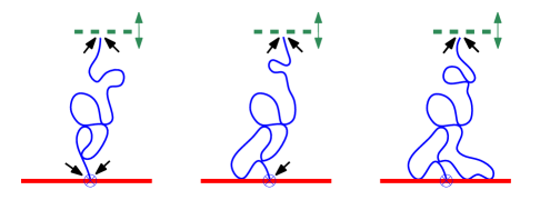
Figure 12: A polymer chain at the $\Theta$-point anchored at a surface, in a bridge configuration in two-dimensions, which corresponds to ordinary boundary conditions as marked by two arrows near the topmost virtual line. Left: Ordinary b.c.’s yield the bridge exponent $\gamma_{b}^{\Theta}(\mathrm{or})$. Middle: Mixed b.c.’s yield the bridge exponent $\gamma^{\Theta}_{b}(\mathrm{o\bullet s})$. Right: Special b.c.’s yield the bridge exponent $\gamma^{\Theta}_{b}(\mathrm{sp})$.

Turning now to bridges, a single bridge at the ordinary transition point can be considered as a TAW rooted at the surface, but with end-point free to move in the bulk, provided it lies in a parallel surface at maximal spacing between the two surfaces (Fig. 12). We obtain from (21) that it can be described as a network with ${\mathcal{V}}=1,$ ${\mathcal{V}}_{S}=1,$ ${\mathcal{N}}=1,$ $n_{1}=0,$ and $n_{1}^{S}=1$, $n_{1}^{b}=1$, and all other $L$-vertex numbers vanishing for $L\geq 2$. This gives the exponent for single ordinary transition bridges as (hereafter dropping $({\rm or})$)

$$\gamma^{\Theta}_{b}=\nu^{\Theta}[2-2x_{1}^{\Theta,S}]=\gamma^{\Theta}_{11}+\nu^{\Theta}=0.$$ (106)

4.3.3 The special transition.

For the special transition, the origin vertex has for surface exponent $x_{1}^{\Theta,S}({\rm sp})$ (Fig. 12). In this way we find the special bridge exponent,

$$\gamma_{b}^{\Theta}({\rm sp})=\nu^{\Theta}[2-x_{1}^{\Theta,S}-x_{1}^{\Theta,S}({\rm sp})]=\frac{4}{7}.$$

From the above, we also obtain the special transition scaling relation [65],

$$\gamma_{b}^{\Theta}({\rm sp})=\frac{1}{2}\left[\gamma^{\Theta}_{11}({\rm sp})+\gamma^{\Theta}_{11}\right]+\nu^{\Theta}.$$ (107)

4.3.4 Mixed boundary conditions.

When the attachment vertex is of mixed ordinary-special type, with exponent $x_{1}^{\Theta,S}({\rm o\bullet s})=1/3$ (Fig. 12), we get

$$\gamma_{1}^{\Theta}({\rm o\bullet s}) = \nu^{\Theta}[2-x_{1}^{\Theta}-x_{1}^{\Theta,S}({\rm o\bullet s})]=\frac{20}{21},$$ (108)

$$\gamma_{b}^{\Theta}({\rm o\bullet s}) = \nu^{\Theta}[2-x_{1}^{\Theta,S}-x_{1}^{\Theta,S}({\rm o\bullet s})]=\frac{8}{21}.$$ (109)

4.3.5 $L$-multi-bridge.

As an application of the scaling theory developed in Section 2.2, i.e., Eqs. (18), (20) and (21), to $\Theta$-point conditions, consider for exemple the simple case depicted in Fig. 7. Assume all chains to be in $\Theta$-point conditions, and all the $L$-bulk single vertices to be local bridge vertices. This $L$-bridge configuration gives rise to configurational exponents,

$$\gamma_{L,b}^{\Theta}(\cdot)=\nu^{\Theta}\left[2L-Lx_{1}^{\Theta,S}-x_{L}^{\Theta,S}(\cdot)\right],$$ (110)

where $(\cdot)$ represents either $({\rm sp})$, or $({\rm o\bullet sp})$, or $({\rm or})$, depending on the boundary conditions. Eqs. (101), (102) (103) and (104) yield the explicit $L$-bridge exponents,

$$\gamma_{L,b}^{\Theta}({\rm sp}) = \frac{2}{21}L(7-L),\,\,\,\gamma_{L,b}^{\Theta}({\rm o\bullet s})=\frac{2}{21}L(5-L),$$ (111)

$$\gamma_{L,b}^{\Theta}({\rm or}) = \frac{2}{21}(3L-L^{2}-2).$$ (112)

5 Numerical results

A number of the scaling relations given above can be compared to recent numerical work in a number of papers. The exponent for bridges at the ordinary transition has been calculated by both series and Monte Carlo methods in two- and three-dimensions by Clisby et al. in [26]. They found $\gamma_{b}(2\textrm{d})=9/16,$ and $\gamma_{b}(3\textrm{d})=0.198352\pm 0.000027.$ These are completely consistent with the scaling relation $\gamma_{b}=\gamma_{11}+\nu$ given in Eq. (6).

At the special transition, the scaling relation for bridges predicts $\gamma_{b}(\textrm{sp})=17/16$ for the two-dimensional case, and $\gamma_{b}(\textrm{sp})\approx 0.746$ for the three-dimensional case. The result for the two dimensional case has been confirmed by a recent series analysis study [13]. Furthermore, the epsilon expansion, given in [65] gives the values $\gamma_{b}(\textrm{sp})=1.164$ and $\gamma_{b}(\textrm{sp})=0.760$ respectively for the exponents in two- and three-dimensions. This is very satisfactory agreement.

For bridges at the theta-point, Beaton et al [13] found $\gamma_{b}^{\Theta}=0.00\pm 0.03$ which is in perfect agreement with the prediction given in Eq. (106) that this exponent should be precisely zero. For $\gamma_{1}^{\Theta}$ Seno and Stella [133] estimated $\gamma_{1}^{\Theta}=0.57\pm 0.09$ based on a Monte Carlo analysis. Series analysis estimates have been given by Foster et al. in [86] of $0.57\pm 0.02$ while Beaton et al. [13] used longer series to estimate $\gamma_{1}^{\Theta}=0.55\pm 0.03.$ All these estimates are in good agreement with the calculation here that gives $\gamma_{1}^{\Theta}=4/7.$

For self-avoiding polygons partly adsorbed at the special transition, the situation presents an interesting subtlety. In two-dimensions, we find from Eq. 26 $x_{2}^{S}(\textrm{sp})=1/3,$ and since $\gamma_{p}(\textrm{sp})=-\nu\,x_{2}^{S}(\textrm{sp})$ and $\nu=3/4$, we obtain the prediction $\gamma_{p}(\textrm{sp})=-1/4.$ In [94] careful series analysis gave the estimate $\widehat{\gamma}_{p}\approx-0.754,$ suggesting that the exact value should be $\widehat{\gamma}_{p}=-3/4.$

This apparent discrepancy arises due to the way that monomer contacts should be counted in the case of the special transition. If a polygon of $N$ sites has $m$ surface contacts, one can either give the polygon a weight 1 or a weight $m.$ In [94] a polygon with $m$ monomers in the surface was given a weight 1. In the ordinary-transition case this makes no difference, as when the surface fugacity $a$ is less than the critical fugacity $a_{c},$ only a microscopic fraction of the $N$ monomers are in the surface. However at the special transition, one expects a typical value $m\propto N^{\phi}=N^{1/2},$ because the crossover exponent is exactly $\phi=1/2$ for any dilute critical $O(n)$ model [17, 18, 83]. Thus, introducing the weight $m$, which corresponds to the number of possible choices of the 2-leg root vertex in the partly adsorbed configuration of the polygon, should change the configuration exponent by $+1/2$. We checked that a reanalysis of the series with weight $m$ yields a configuration exponent $-0.254$ close to the expected $-1/4$, which accounts for the apparent discrepancy.

Moreover, we remark that Eq. 85 gives the mixed boundary 2-leg exponent $x_{2}^{S}(\textrm{or}\bullet\textrm{sp})=1$, which in turn yields $\gamma_{p}(\textrm{or}\bullet\textrm{sp})=-\nu\,x_{2}^{S}(\textrm{or}\bullet\textrm{sp})=-3/4$. It is thus tantalising to conclude that the measured value $\widehat{\gamma}_{p}\approx-0.754$ in [94] precisely corresponds to the prediction $\widehat{\gamma}_{p}=\gamma_{p}(\textrm{or}\bullet\textrm{sp})$ instead of $\gamma_{p}(\textrm{sp})$. A partly adsorbed polygon configuration, when counted with weight 1, can in fact be associated with that of a polygon with mixed boundary conditions, by viewing the leftmost boundary vertex of the polygon as a point where the boundary conditions change from ordinary to special (or, equivalently, by seeing the rightmost boundary vertex as the point where the boundary conditions change from special to ordinary).

6 Conclusion

We have given several examples showing how the theory of the critical behaviour of $d$-dimensional polymer networks [50, 71, 55] can be extended to the situation of bridges where the chains lie between two parallel hyper-planes. We have generalized the findings of our earlier work [65] to the case of multi-bridges where several multi-chain vertices are in local bridge configurations. The exact scaling laws for two-dimensional confined polymer networks made of either self-avoiding walks, or mutually-avoiding walks, or $\Theta$-point walks, either at the ordinary, or special, or mixed surface transitions, are given. All sets of multiple-path Euclidean scaling exponents are described from a unified SLE perspective, via the canonical use of the fundamental KPZ relation between Euclidean and Liouville quantum gravity exponents. We also give supportive results based on series and Monte Carlo enumeration data.

References

References

- [1] M Aizenman, B Duplantier and A Aharony, Path-Crossing Exponents and the External Perimeter in 2D Percolation, Phys. Rev. Lett. 83, 1359–1362, 1999.
- [2] M N Barber, Scaling Relations for Critical Exponents of Surface Properties of Magnets, Phys. Rev. B 8 407–9, 1973.
- [3] J Barral, X Jin, R Rhodes, and V Vargas, Gaussian multiplicative chaos and KPZ duality, Comm. Math. Phys. 323, 451–485, 2013.
- [4] M T Batchelor, D. Bennett-Wood and A. L. Owczarek, Two-dimensional polymer networks at a mixed boundary: Surface and wedge exponents, Eur. Phys. Journal B 5, 139–142, 1998.
- [5] M T Batchelor and H W J Blöte, Conformal invariance and critical behavior of the model on the honeycomb lattice, Phys. Rev. B 39, 2391–2402, 1989.
- [6] M T Batchelor and J Suzuki, Exact solution and surface critical behaviour of an model on the honeycomb lattice, J. Phys. A.: Math. Gen. 26, L729–L735, 1993.
- [7] M T Batchelor and C M Yung, Exact Results for the Adsorption of a Flexible Self-Avoiding Polymer Chain in Two Dimensions, Phys. Rev. Lett. 74, 2026–2029, 1995.
- [8] M T Batchelor and C M Yung, Surface critical behaviour of the honeycomb loop model with mixed ordinary and special boundary conditions, J. Phys. A: Math. Gen. 28, L421-L426, 1995.
- [9] M Bauer, D Bernard, and K Kytölä, Multiple Schramm-Loewner evolutions and statistical mechanics martingales, J. Stat. Phys. 120(5-6):1125–1163, 2005.
- [10] R Bauerschmidt and G Slade, Mean-field tricritical polymers, https://arxiv.org/pdf/1911.00395.
- [11] R Bauerschmidt, M Lohmann and G Slade, Three-dimensional tricritical spins and polymers, J. Math. Phys. 61, 033302, 2020.
- [12] N R Beaton, M Bousquet-Mélou, J de Gier, H Duminil-Copin and A J Guttmann, The critical fugacity for surface adsorption of self-avoiding walks on the honeycomb lattice is Commun. Math. Phys. 326, 727—754, 2014.
- [13] N R Beaton, A J Guttmann, and I Jensen, Two-dimensional interacting self-avoiding walks: new estimates for critical temperatures and exponents, https://arxiv.org/abs/1911.05852.
- [14] V Beffara, E Peltola, and H Wu, On the uniqueness of global multiple SLEs, 2018. https://arxiv.org/abs/1801.07699
- [15] M. Benhamou and G. Mahoux, Multiplicative renormalization of continuous polymer theories, in good and solvents, up to critical dimensions, J. Physique 47, 559–568, 1986.
- [16] J-E Bourgine, K Hosomichi, I Kostov, Boundary transitions of the ) model on a dynamical lattice, Nucl. Phys. B 832 [FS] 462–499, 2010.
- [17] T W Burkhardt, E Eisenriegler and I Guim, Conformal theory of energy correlations in the semi-infinite two-dimensional model, Nucl. Phys. B 316, 559–572, 1989.
- [18] T W Burkhardt and E Eisenriegler, Conformal theory of the two-dimensional model with ordinary, extraordinary, and special boundary conditions, Nucl. Phys. B 424 [FS] 48–504, 1994.
- [19] S Caracciolo, M Gherardi, M Papinutto and A Pelissetto, Geometrical properties of two-dimensional interacting self-avoiding walks at the -point, J. Phys. A: Math. Theor. 44, 115004 (17pp), 2011.
- [20] J L Cardy, Conformal invariance and surface critical behavior, Nucl. Phys. B 240 [FS12]] 514–532, 1984.
- [21] J L Cardy, H W Hamber, Heisenberg model close to , Phys. Rev. Lett. 45, 499-501, 1980; Erratum Phys. Rev. Lett. 45, 1217, 1980.
- [22] D Chelkak and S Smirnov, Universality in the 2D Ising model and conformal invariance of fermionic observables, Invent. math. 189:515–580, 2012.
- [23] N Clisby, Calculation of the connective constant for self-avoiding walks via the pivot algorithm, J. Phys. A: Math. Theor. 46 245001, 2013.
- [24] M Daoud, J P Cotton, B Farnoux, G Jannink, G Sarma, H Benoit, C Duplessix, C Picot, P-G de Gennes, Solutions of Flexible Polymers. Neutron Experiments and Interpretation, Macromolecules 8(6), 804–818, 1975.
- [25] M Daoud, G Jannink, Temperature-concentration diagram of polymer solutions, J. Physique 37 (7-8), 973–979, 1976.
- [26] N Clisby, A R Conway and A J Guttmann, Three-dimensional terminally attached self-avoiding walks and bridges, J. Phys. A.: Math. Theor. 49 015004, 2016.
- [27] J. des Cloizeaux, The Lagrangian theory of polymer solutions at intermediate concentrations, J. Phys. France 36, 281-291, 1975.
- [28] J. des Cloizeaux, A method for determining by direct renormalization the properties of long polymers in solutions, J. Physique Lett. 41, 151-155, 1980.
- [29] J. des Cloizeaux, Polymers in solutions: principles and applications of a direct renormalization method, J. Physique 42, 635-652, 1981.
- [30] J des Cloizeaux and G Jannink, Polymers in Solution, Their Modelling and Structure, Oxford University Press, Oxford, 1989.
- [31] A Coniglio, N Jan, I Majid, H E Stanley, Conformation of a polymer chain at the point: Connection to the external perimeter of a percolation cluster, Phys Rev B 35 3617–3620, 1987.
- [32] F David, Conformal field theories coupled to 2-D gravity in the conformal gauge, Mod. Phys. Lett. A 3, 1651–1656, 1988.
- [33] H W Diehl, Field-theoretical approach to critical behaviour at surfaces, in Phase Transitions and Critical Phenomena, Vol 10, eds. C Domb and M S Green, Academic Press, London and New York, 76-267, 1986.
- [34] H W Diehl and S Dietrich, Scaling laws and surface exponents from renormalization group equations, Phys. Lett. 80 A, 408–412, 1980.
- [35] H W Diehl and S Dietrich, Field-theoretical approach to multicritical behavior near free surfaces, Phys. Rev. B 24, 2878–2880(R), 1981.
- [36] H W Diehl and E Eisenriegler, Irrelevance of Surface Anisotropies for Critical Behavior Near Free Surface, Phys. Rev. Lett. 48, 1767, 1982.
- [37] H W Diehl and E Eisenriegler, Effects of surface exchange anisotropies on magnetic critical and multicritical behavior at surfaces, Phys. Rev. B 30, 300, 1984.
- [38] H W Diehl, S Dietrich and E Eisenriegler, Universality, irrelevant surface operators, and corrections to scaling in systems with free surfaces and defect planes, Phys. Rev B 27, 2937–2954, 1983.
- [39] J Distler and H Kawai, Conformal field theory and 2D quantum gravity, Nucl. Phys. B 321, 509–527, 1989.
- [40] J Dubail, J L Jacobsen, and H Saleur, Exact Solution of the Anisotropic Special Transition in the Model in Two Dimensions, Phys. Rev. Lett. 103, 145701, 2009.
- [41] J Dubail, J L Jacobsen, and H Saleur, Conformal boundary conditions in the critical model and dilute loop models, Nucl. Phys. B 827, 457–502, 2010.
- [42] J Dubail, Conditions aux bords dans des théories conformes non-unitaires, PhD Thesis, 2010, https://tel.archives-ouvertes.fr/tel-00555624/document
- [43] J Dubédat, SLE Martingales and Duality, Ann. Probab. 33(1), 223–243, 2005.
- [44] J Dubédat, Commutation relations for Schramm-Loewner evolutions, Commun. Pure Appl. Math. 60, 1792–1847, 2007.
- [45] H Duminil-Copin, S Smirnov, The connective constant of the honeycomb lattice equals , Ann. Math. 175 1653-1665, 2012.
- [46] B Duplantier, Lagrangian tricritical theory of polymer chain solutions near the -point, J. Physique 43, 991-1019, 1982.
- [47] B Duplantier, Tricritical Polymer Chains in or below Three Dimensions, Europhys. Lett. 1, 491–498, 1986.
- [48] B Duplantier, Dimensional renormalizations of polymer theory, J. Phys. France 47, 569–579, 1986.
- [49] B Duplantier, Direct or dimensional renormalizations of the tricritical polymer theory, J. Phys. France 47, 745–756, 1986.
- [50] B Duplantier, Polymer Network of Fixed Topology: Renormalization, Exact Critical Exponent in Two Dimensions, and , Phys. Rev. Lett. 57, 941–944, 1986.
- [51] B Duplantier, Critical exponents of Manhattan Hamiltonian walks in two dimensions, from Potts and models. J. Stat. Phys. 49, 411–431, 1987.
- [52] B Duplantier, Polymer Networks at the Tricritical -Point, Europhys. Lett. 7, 677–682, 1988.
- [53] B Duplantier, Intersections of Random walks. A Direct Renormalization Approach, Commun. Math. Phys. 117, 279–329, 1988.
- [54] B Duplantier, Two-dimensional fractal geometry, critical phenomena and conformal invariance, Phys. Rep. 184, 229–257, 1989.
- [55] B Duplantier, Statistical Mechanics of Polymer Networks of Any Topology, J. Stat. Phys. 54, 581–680, 1989.
- [56] B Duplantier, Random Walks and Quantum Gravity in Two Dimensions, Phys. Rev. Lett. 81, 5489–5492, 1998.
- [57] B Duplantier, Two-Dimensional Copolymers and Exact Conformal Multifractality, Phys. Rev. Lett. 82, 880–883, 1999.
- [58] B Duplantier, Harmonic Measure Exponents for Two-Dimensional Percolation, Phys. Rev. Lett. 82, 3940–3943, 1999.
- [59] B Duplantier, Conformally Invariant Fractals and Potential Theory, Phys. Rev. Lett. 84, 1363–1367, 2000.
- [60] B Duplantier, Higher conformal multifractality, J. Stat. Phys. 110, 691–738, 2003.
- [61] B Duplantier, Conformal fractal geometry & boundary quantum gravity, in Fractal Geometry and Applications: A Jubilee of Benoît Mandelbrot, Proc. Symposia Pure Math. Vol. 72, Part 2, Michel L Lapidus and Machiel van Frankenhuijsen Editors, 365-482, 2004 (AMS, Providence, R.I.).
- [62] B Duplantier, Conformal Random Geometry, in Mathematical Statistical Physics, Les Houches Summer School LXXXIII, F. Dunlop, F. den Hollander, A. van Enter and J. Dalibard, eds., pp. 101-217, Elsevier B. V., 2006.
- [63] B Duplantier, A rigorous perspective on Liouville quantum gravity and the KPZ relation. In S. Ouvry, J. Jacobsen, V. Pasquier, D. Serban, and L. Cugliandolo, editors, Exact methods in low-dimensional statistical physics and quantum theory (Les Houches Summer School LXXXIX, 2008), pages 529–561. Oxford Univ. Press, Oxford, 2010.
- [64] B Duplantier, Liouville Quantum Gravity, KPZ Relation and Schramm-Loewner Evolution, Proceeding of the International Congress of Mathematicians, Seoul 2014, SY Jang et al. eds., Vol. III, 1035–1061, 2014, https://www.mathunion.org/fileadmin/ICM/Proceedings/ICM2014.3/ICM2014.3.pdf.
- [65] B Duplantier and A J Guttmann, New scaling laws for self-avoiding walks: bridges and worms, J. Stat. Mech. (2019) 104010, special issue dedicated to the Memory of Vladimir Rittenberg. https://doi.org/10.1088/1742-5468/ab4584.
- [66] B Duplantier and I K Kostov, Conformal Spectra of Polymers on a Random Surface, Phys. Rev. Lett. 61, 1433–1437, 1988.
- [67] B Duplantier and I K Kostov, Geometrical critical phenomena on a random surface of arbitrary genus, Nucl. Phys. B 340 [FS], 491–541, 1990.
- [68] B Duplantier and K-H Kwon, Conformal Invariance and Intersections of Random Walks, Phys. Rev. Lett. 61, 2514–2517, 1988.
- [69] B Duplantier, J Miller and S Sheffield, Liouville quantum gravity as a mating of trees, Astérisque, Société Mathématique de France, Paris (in press), 2020, https://arxiv.org/abs/1409.7055. 2014.
- [70] B Duplantier, R Rhodes, S Sheffield and V Vargas, Renormalization of Critical Gaussian Multiplicative Chaos and KPZ Relation, Commun. Math. Phys. 330, 283–330, 2014.
- [71] B Duplantier and H Saleur, Exact Surface and Wedge Exponents for Polymers in Two Dimensions, Phys. Rev. Lett. 57, 3179–3182, 1986.
- [72] B Duplantier and H Saleur, Exact Tricritical Exponents for Polymers at the -Point in Two Dimensions, Phys. Rev. Lett. 59, 539–542, 1987.
- [73] B Duplantier and H Saleur, Duplantier and Saleur Reply, Phys. Rev. Lett. 60, 1204, 1988.
- [74] B Duplantier and H Saleur, Duplantier and Saleur Reply, Phys. Rev. Lett. 61, 1521, 1988.
- [75] B Duplantier and H Saleur, Stability of the Polymer -Point in Two Dimensions, Phys. Rev. Lett. 62, 1368–1371, 1989.
- [76] B Duplantier and H Saleur, Duplantier and Saleur Reply, Phys. Rev. Lett. 62, 2641, 1989.
- [77] B Duplantier and S Sheffield, Duality and the Knizhnik-Polyakov-Zamolodchikov Relation in Liouville Quantum Gravity, Phys. Rev. Lett. 102, 150603, 2009.
- [78] B Duplantier and S Sheffield, Liouville quantum gravity and KPZ, Invent. math. 185 (2), 333–393, 2011.
- [79] B Duplantier and S Sheffield, Schramm-Loewner Evolution and Liouville Quantum Gravity, Phys. Rev. Lett. 107, 131305, 2011.
- [80] B Dyhr, M Gilbert, T Kennedy, G F Lawler and S Passon, The self-avoiding walk spanning a strip, J. Stat. Phys. 144, 1–22, 2011.
- [81] S F Edwards, The statistical mechanics of polymers with excluded volume, Proc. Phys. Soc. 85 613–624, 1965.
- [82] E Eisenriegler, Polymers near Surfaces, World Scientific, Singapore, 1993.
- [83] P Fendley and H Saleur, Exact theory of polymer adsorption in analogy with the Kondo problem, J. Phys. A: Math. Gen. 27 L789–L796, 1994.
- [84] C von Ferber, Y Holovatch, Copolymer networks and stars: Scaling exponents, Phys. Rev. E 56, 6370–6386, 1997.
- [85] P. Flory, Principles of Polymer Chemistry, Cornell University Press, 1953.
- [86] D P Foster, E Orlandini, M C Tesi, Surface critical exponents for models of polymer collapse and adsorption: the universality of the and points, J. Phys. A: Math. Gen. 25, L1211–L1217, 1992.
- [87] D S Gaunt, J E G Lipson, S G Whittington and M K Wilkinson, Lattice models of branched polymers: uniform combs in two dimensions, J. Phys. A: Math. Gen. 19:L811-816, 1986.
- [88] P-G de Gennes, Exponents for the excluded volume problem as derived by the Wilson method, Phys. Lett. 38, 339–340, 1972.
- [89] P-G de Gennes, Collapse of a polymer chain in poor solvents, J. Phys. (Paris) Lett. 36 (3), 55–57, 1975.
- [90] P-G de Gennes, Collapse of a flexible polymer chain II, J. Phys. (Paris) Lett. 39 (17), 299–301, 1978.
- [91] P-G de Gennes, Scaling concepts in polymer physics, Cornell University, 1979.
- [92] K Graham, On multiple Schramm-Loewner evolutions, J. Stat. Mech. Theory Exp., (3):P03008, 21, 2007.
- [93] I Guim and T W Burkhardt, Transfer-matrix study of the adsorption of a flexible self-avoiding polymer chain in two dimensions, J. Phys. A: Math. Gen. 22 1131–1140, 1989.
- [94] A J Guttmann, E J Janse van Rensburg, I Jensen and S G Whittington, Polygons pulled from an adsorbing surface, J Phys A: Math Theor. 51 074001 (30pp), 2018.
- [95] E Gwynne, N Holden and X Sun, Mating of trees for random planar maps and Liouville quantum gravity: a survey, https://arxiv.org/abs/1910.04713.
- [96] J M Hammersley, Percolation processes II. The connective constant, Proc. Camb. Phil. Soc. 53, 642-645, 1957.
- [97] . J M Hammersley, and D J A Welsh, Further results on the rate of convergence to the connective constant of the hypercubical lattice, The Quarterly Journal of Mathematics. Oxford 13 108–110, 1962. J M Hammersley, The number of polygons on a lattice, Proceedings of the Cambridge Philosophical Society 57, 516–523, 1961. R Hegger and P Grassberger, J. Phys. A: Math. Gen 27, 4069–4081, 1994.
- [98] W Kager and B Nienhuis, A guide to stochastic Löwner evolution and its applications, J. Stat. Phys. 115, 1149–1229, 2004.
- [99] V A Kazakov, Ising model on a dynamical planar random lattice: Exact solution, Phys. Lett. A 119, 140–144, 1986.
- [100] V G Knizhnik, A M Polyakov and A B Zamolodchikov, Fractal structure of 2d-quantum gravity, Mod. Phys. Lett. A 3, 819–826 (1988); see also A M Polyakov, Quantum gravity in two dimensions, Mod. Phys. Lett. A 2, 893–898 (1987).
- [101] M J Kozdron and G F Lawler, The configurational measure on mutually avoiding SLE paths, in Universality and renormalization, volume 50 of Fields Inst. Commun., 199–224. Amer. Math. Soc., Providence, RI, 2007.
- [102] K Kytölä and E Peltola, Pure partition functions of multiple SLEs, Commun. Math. Phys. 346(1):237–292, 2016.
- [103] G F Lawler, Partition functions, loop measure, and versions of SLE, J. Stat. Phys. 134(5-6):813–837, 2009.
- [104] G F Lawler, W Werner, Intersection exponents for planar Brownian motion, Ann. Probab., 27,1601–1642, 1999.
- [105] G F Lawler, W Werner, Universality for conformally invariant intersection exponents, J. European Math. Soc. 2, 291–328, 2000.
- [106] G F Lawler, O Schramm and W Werner, Values of Brownian intersection exponents, I: Half-plane exponents, Acta Math. 187, 237–273, 2001.
- [107] G F Lawler, O Schramm and W Werner, Values of Brownian intersection exponents, II: Plane exponents, Acta Math. 187, 275–308, 2001.
- [108] G F Lawler, O Schramm and W Werner, Values of Brownian intersection exponents III : two-sided exponents, Ann. Inst. Henri Poincaré Probab. Stat 38(1), 109–123, 2002.
- [109] G F Lawler, O Schramm and W Werner, The dimension of the planar Brownian frontier is 4/3, Math. Res. Lett. 8, 401–411, 2001.
- [110] G F Lawler, O Schramm and W Werner, On the scaling limit of planar self-avoiding walk, in Fractal geometry and applications: a jubilee of Benoît Mandelbrot, Part 2, 339–364, Proc. Sympos. Pure Math., 72, Part 2, Amer. Math. Soc., Providence, RI, 2004.
- [111] J E G Lipson, S G Whittington, M K Wilkinson, J L Martin, and D S Gaunt, A lattice model of uniform star polymers, J. Phys. A 18:L469-L473, 1985.
- [112] B B Mandelbrot, The Fractal Geometry of Nature, WH Freeman and Co, San Francisco, 1982.
- [113] H Meirovitch and H A Lim, -Point Exponents of Polymers in , Phys. Rev. Lett. 62, 2640, 1989.
- [114] J Miller and S Sheffield, Imaginary geometry II, reversibility of SLE for , Ann. Probab. 44(3), 1647–1722, 2016.
- [115] J Miller, H Wu, Intersections of SLE Paths: the double and cut point dimension of SLE, Probab. Theory Relat. Fields 167, 45–105, 2017.
- [116] B Nienhuis, Exact Critical Point and Critical Exponents of Models in Two Dimensions, Phys. Rev. Lett. 49 1062-1065, 1982; Critical Behavior of Two-Dimensional Spin Models and Charge Asymmetry in the Coulomb Gas, J. Stat. Phys. 34, 731–761, 1984.
- [117] B Nienhuis, Two-dimensional critical phenomena and the Coulomb Gas, in Phase Transitions and Critical Phenomena, Vol. 11, C. Domb and J.L. Lebowitz, eds. (Academic Press, London, 1987).
- [118] K Ohno and K Binder, Scaling theory of star polymers and general polymer networks in bulk and semi-infinite good solvents, J. Phys. France 49, 1329–1351, 1988.
- [119] E Peltola, Toward a conformal field theory for Schramm-Loewner evolutions, J. Math. Phys. 60, 103305, 2019, Special Collection: International Congress on Mathematical Physics (ICMP) 2018, Montréal.
- [120] E Peltola and H Wu, Global and Local Multiple SLEs for and Connection Probabilities for Level Lines of GFF, Commun. Math. Phys. 366, 469–536, 2019.
- [121] A M Polyakov, Quantum geometry of bosonic strings, Phys. Lett. B 103, 207-210, 1981.
- [122] P H Poole, A Coniglio, N Jan, and H E Stanley, Universality Classes for the and Points, Phys. Rev. Lett. 60, 1203, 1988.
- [123] R Rhodes and V Vargas, KPZ formula for log-infinitely divisible multifractal random measures, ESAIM Prob. Stat. 15, 358–371, 2011.
- [124] H Saleur, New exact critical exponents for 2d self-avoiding walks, J. Phys. A: Math. Gen. 19, L807–810, 1986.
- [125] H Saleur, Conformal invariance for polymers and percolation, J. Phys. A: Math. Gen. 20, 455–470, 1987.
- [126] H Saleur and B Duplantier, Exact Determination of the Percolation Hull Exponent in Two Dimensions, Phys. Rev. Lett. 58, 2325–2328, 1987.
- [127] L Schäfer, Excluded Volume Effects in Polymer Solutions, as Explained by the Renormalization Group, Springer, Berlin-Heidelberg, 1999.
- [128] L Schäfer, C von Ferber, U Lehr, and B Duplantier, Renormalization of polymer networks and stars, Nucl. Phys. B [FS] 374(3), 473–495, 1992.
- [129] L Schäfer and T A Witten, Renormalized field theory of polymer solutions. I Scaling laws, J. Chem. Phys. 66, 2121–2130 ,1977.
- [130] L Schäfer and T A Witten, Renormalized field theory of polymer solutions : extension to general polydispersity, J. Physique 41, 459–473, 1980.
- [131] O Schramm, Scaling limits of loop-erased random walks and uniform spanning trees, Isr. J. Math. 118 221–288, 2000.
- [132] F Seno, A Stella, C Vanderzande, Universality Class of the Point of Linear Polymers, Phys. Rev. Lett. 61, 1520, 1988.
- [133] F Seno, A Stella, Surface Exponents for a Linear Polymer at the point, Europhys. Lett. 7,(7) 605–610, 1988.
- [134] F Seno, A Stella, C Vanderzande, Self-Avoiding Walks in the Presence of Strongly Correlated, Annealed Vacancies, Phys. Rev. Lett. 65, 2897–2900, 1990.
- [135] S Sheffield, Conformal weldings of random surfaces: SLE and the quantum gravity zipper, Ann. Probab. 44(5) 3474–3545, 2016.
- [136] S Smirnov, Critical percolation in the plane: conformal invariance, Cardy’s formula, scaling limits, C. R. Acad. Sci. Paris Sér. I Math., 333, no. 3, 239–244, 2001.
- [137] S Smirnov, Conformal invariance in random cluster models. I. Holomorphic fermions in the Ising model, Ann. of Math. 172(2), 1435–1467, 2010.
- [138] A L Stella, F Seno, C Vanderzande, Boundary Critical Behavior of Self-Avoiding Walks on Correlated and Uncorrelated Vacancies, J. Stat. Phys. 73, 21-46, 1993.
- [139] C Vanderzande, A L Stella, and F Seno, Percolation, the Special Point, and the – Universality Puzzle, Phys. Rev. Lett. 67, 2757–2760, 1991.
- [140] É Vernier, J L Jacobsen and H Saleur, A new look at the collapse of two-dimensional polymers, J. Stat. Mech. 2015 P09001 (35pp), 2015.
- [141] S O Warnaar, M T Batchelor and B Nienhuis, Critical properties of the Izergin- Korepin and solvable models and their related quantum spin chains, J. Phys. A: Math. Gen. 25, 3077–3095, 1992.
- [142] M Wang and H Wu, Remarks on the intersection of SLE curve with the real line, https://arxiv.org/abs/1507.00218.
- [143] W Werner, Lectures on random planar curves and Schramm-Loewner evolution. École d’Été de Probabilités de Saint-Flour, Lecture Notes in Math. 1840 107–195, 2004, Springer, Berlin.
- [144] W Werner, Girsanov transformation for SLE processes, intersection exponents and hiding exponent. Ann. Fac. Sci. Toulouse Math. (6), tome 13, no 1, 121–147, 2004. http://www.numdam.org/article/AFST_2004_6_13_1_121_0.pdf
- [145] M K Wilkinson, D S Gaunt, J E G Lipson, and S G Whittington, Lattice models of branched polymers: statistics of uniform stars, J Phys A: Math Gen, 19, 789-796, 1986.
- [146] K G Wilson and M E Fisher, Critical Exponents in 3.99 Dimensions, Phys. Rev. Lett. 28, 240-243, 1972.
- [147] T A Witten and L Schäfer, Two critical ratios in polymer solutions, J Phys. A: Math. Gen. 11, 1843–1854, 1978.
- [148] H Wu, Polychromatic Arm Exponents for the Critical Planar FK-Ising Model, J. Stat. Phys. 170, 1177–1196, 2018.
- [149] H Wu and D Zhan, Boundary Arm Exponents for SLE, Electron. J. Probab. 22, paper no. 89, 26 pp., 2017.
- [150] C M Yung, M T Batchelor, model on the honeycomb lattice via reflection matrices: Surface critical behaviour, Nucl. Phys. B 453, 552–580, 1995.
- [151] D Zhan, Duality of chordal SLE, Invent. math. 174, 309–353, 2008.