Modulational instability of ion-acoustic waves and associated envelope solitons in a multi-component plasma

Abstract

A generalized plasma model having warm ions, iso-thermal electrons, super-thermal electrons and positrons is considered to theoretically investigate the modulational instability (MI) of ion-acoustic waves (IAWs). A standard nonlinear Schrödinger equation is derived by applying reductive perturbation method to study the MI of IAWs. It is observed that the MI criteria of the IAWs are significantly modified by various plasma parameters. The present results should be useful in understanding the conditions for MI of IAWs which are relevant to both space and laboratory plasma system.

1 Introduction

The co-existence of electrons and positrons in an electron-positron-ion (EPI) plasma medium (EPIPM) which creates a new field of research for the physicists to understand the nonlinear collective features of EPIPM by considering waves dynamics, namely, ion-acoustic (IA) waves (IAWs) [1, 2, 3, 4, 5, 6, 7], positron-acoustic waves (PAWs), electron-acoustic waves (EAWs) [8], and IA rogue waves (IARWs) as well as their associated nonlinear structures such as solitons [4, 5], dark and bright envelope solitons [2], shocks, rogue waves [6], double layers has been identified by the THEMIS mission [9] and Viking Satellite [10] in both space (viz., Saturn’s magnetosphere [1], early universe [4], solar atmosphere [1], active galactic nuclei [11], pulsar magnetosphere [4], and polar regions of neutron stars [12], etc.) and laboratory environments (viz., high intensity laser irradiation [4], semiconductor plasmas [11], hot cathode discharge [4], and magnetic confinement systems [11], etc.).

Two temperature electrons (hot and cold) have been identified by the Voyager PLS [13] and Cassini CAPS [14] observations in Saturn’s magnetosphere, and successively have been verified by several satellite missions, viz., Viking Satellite [10], FAST Auroral Snapshot (FAST) at the auroral region [15] and THEMIS mission [9], and are governed by the super-thermal kappa/$\kappa$-distribution rather than well-known Maxwellian distribution, and have also been considered by many authors for analysing the propagation of the nonlinear electrostatic waves [1, 3, 8, 16]. The super-thermal parameter ($\kappa$) in $\kappa$-distribution represents super-thermality of plasma species, and the small values of $\kappa$ determine the large deviation of the plasma species from thermally equilibrium state of plasma system while for the large values of $\kappa$, the plasma system coincides with the Maxwellian distribution. Shahmansouri and Alinejad [5] considered three components plasma model having two temperature super-thermal electrons and cold ions, and investigated IA solitary waves, and confirmed that the existence of both compressive and rarefactive solitary structures in presence of the two temperature super-thermal electrons. Baluku and Helberg theoretically and numerically analyzed IA solitons in presence of two temperature super-thermal electrons. Panwar et al. [1] have demonstrated IA cnoidal waves in a three components plasma medium having inertial cold ion and inertialess two temperature $\kappa$-distributed electrons, and found that cold electron’s super-thermality increases the height of the cnoidal wave.

The MI of wave packets has been considered the basic platform for the formation of bright and dark envelope solitons in plasmas, and has also been mesmerized a number of authors to investigate the MI as well as bright and dark envelope solitons in inter-disciplinary field of nonlinear-sciences, viz., oceanic wave [6], fibre telecommunications [2], optics [6], and space plasma [3], etc. The intricate mechanism of the MI of various waves (viz., IAWs, EAWs, and PAWs [17], etc.) and the formation of the electrostatic envelope solitonic solitons has been governed by the standard nonlinear Schrödinger equation (NLSE) [18, 19, 20, 21, 22]. Kourakis and Shukla [2] investigated the MI of the IAWs in a super-thermal plasma having inertial cold ion and inertialess cold and hot electrons. Alinejad et al. [3] studied the stability conditons of the IAWs in presence of the super-thermal electrons, and found that the stable region of the IAWs decreases with the number density of the cold electrons. Ahmed et al. [22] studied the stability of IAWs, and observed that the critical wave number $k_{c}$ decreases with the increase in the value of $\kappa$.

The manuscript is organized in the following order: The governing equations of plasma model are presented in Sec. 2. The derivation of NLSE by using reductive perturbation method (RPM) is represented in Sec. 3. The MI of IAWs is given in Sec. 4. Envelope solitons are provided in Sec. 5. The results and discussion is given in Sec. 6. Finally, the conclusion is presented in Sec. 7.

2 Governing Equations

We consider a four component unmagnetized plasma model consisting of warm ions (with charge $q_{+}=Z_{+}e$; mass $m_{+}$), $\kappa$-distributed super-thermal electrons (with charge $q_{e1}=-e$; mass $m_{e1}$), iso-thermal electrons (with charge $q_{e2}=-e$; mass $m_{e2}$), and super-thermal $\kappa$-distributed positrons (with charge $q_{p}=e$; mass $m_{p}$). The overall charge neutrality condition for this plasma model can be written as $Z_{+}n_{+0}+n_{p0}=n_{e10}+n_{e20}$; where $n_{+0}$, $n_{p0}$, $n_{e10}$, and $n_{e20}$ are the equilibrium number densities of warm ions, super-thermal positrons and electron, and iso-thermal electrons. Now, the basic set of normalized equations can be written in the following form

$$\frac{\partial n_{+}}{\partial t}+\frac{\partial}{\partial x}(n_{+}u_{+})=0,$$ (1)

$$\frac{\partial u_{+}}{\partial t}+u_{+}\frac{\partial u_{+}}{\partial x}+\alpha n_{+}\frac{\partial n_{+}}{\partial x}=-\frac{\partial\phi}{\partial x},$$ (2)

$$\frac{\partial^{2}\phi}{\partial x^{2}}+n_{+}=\mu_{1}n_{e1}+\mu_{2}n_{e2}-(\mu_{1}+\mu_{2}-1)n_{P},\$$ (3)

where $n_{+}$ is the number density of inertial warm ions normalized by its equilibrium value $n_{+0}$; $u_{i}$ is the ion fluid speed normalized by the IAW speed $C_{+}=\sqrt{Z_{+}k_{B}T_{e1}/m_{+}}$ (with $T_{e1}$ being the $\kappa$-distributed electron temperature, $m_{i}$ being the ion rest mass, and $k_{B}$ being the Boltzmann constant); $\phi$ is the electrostatic wave potential normalized by $k_{B}T_{e1}/e$ (with $e$ being the magnitude of single electron charge); the time and space variables are normalized by $\omega_{p+}=\sqrt{4\pi e^{2}Z_{+}^{2}n_{+0}/m_{+}}$ and $\lambda_{D+}=\sqrt{k_{B}T_{e1}/4\pi e^{2}Z_{+}n_{+0}}$, respectively. The pressure term of the ion can be written as $P_{+}=P_{+0}(N_{+}/n_{+0})^{\gamma}$ with $P_{+0}=n_{+0}k_{B}T_{+}$ being the equilibrium pressure of the ion, and $T_{+}$ being the temperature of warm ion, and $\gamma=(N+2)/N$ (where $N$ is the degrees of freedom and for one-dimensional case $N=1$, and then $\gamma=3$). Other parameters are defined as $\alpha=3T_{+}/Z_{+}T_{e1}$, $\mu_{1}=n_{e10}/Z_{+}n_{+0}$, $\mu_{2}=n_{e20}/Z_{+}n_{+0}$, and $\mu_{p}=n_{p0}/Z_{+}n_{+0}$.

The expression for number density of super-thermal electron following the $\kappa$-distribution [3] can be expressed as

$$n_{e1}=\left[1-\frac{\phi}{(\kappa-3/2)}\right]^{(-\kappa+1/2)}$$

$$=1+F_{1}\phi+F_{2}\phi^{2}+F_{3}\phi^{3}+\cdot\cdot\cdot,$$ (4)

where

$$F_{1}=(2\kappa-1)/(2\kappa-3),$$

$$F_{2}=[(2\kappa-1)(2\kappa+1)]/2(2\kappa-3)^{2},$$

$$F_{3}=[(2\kappa-1)(2\kappa+1)(2\kappa+3)]/6(2\kappa-3)^{3}.\$$

The expression for number density of super-thermal positron following the $\kappa$-distribution [3] can be expressed as

$$n_{p}=\Big{[}1+\frac{\delta\phi}{(\kappa-3/2)}\Big{]}^{(-\kappa+1/2)}$$

$$=1-F_{4}\phi+F_{5}\phi^{2}-F_{6}\phi^{3}+\cdot\cdot\cdot,$$ (5)

where $F_{4}=F_{1}\delta$, $F_{5}=F_{2}\delta^{2}$, $F_{6}=F_{3}\delta^{3}$, and $\delta=T_{e1}/{T_{p}}$ (with $T_{p}$ is the super-thermal positron temperature). The expression for the number density of iso-thermal electron can be expressed as

$$n_{e2}=\exp(\lambda\phi)=1+\lambda\phi+\frac{\lambda^{2}}{2}\phi^{2}+\frac{\lambda^{3}}{6}\phi^{3}+\cdot\cdot\cdot,$$ (6)

where $\lambda=T_{e1}/T_{e2}$ (with $T_{e1}>T_{e2}$). Now, by substituting Eqs. (4)- (6) into Eq. (3), and expanding up to third order in $\phi$, we get

$$\frac{\partial^{2}\phi}{\partial x^{2}}+n_{+}=1+F_{7}\phi+F_{8}\phi^{2}+F_{9}\phi^{3}+\cdot\cdot\cdot,$$ (7)

where

$$F_{7}=\mu_{1}F_{1}+\mu_{2}\lambda+(\mu_{1}+\mu_{2}-1)F_{4},$$

$$F_{8}=\mu_{1}F_{2}+\mu_{2}\lambda^{2}/2+(\mu_{1}+\mu_{2}-1)F_{5},$$

$$F_{9}=\mu_{1}F_{3}+\mu_{2}\lambda^{3}/6+(\mu_{1}+\mu_{2}-1)F_{6}.\$$

The terms containing $F7$, $F8$, and $F9$ in the right-hand side of Eq. (7) are the contribution of inertialess electrons and positrons.

3 Derivation of the NLSE

We can employ the RPM to derive the NLSE and hence to study the MI of IAWs. So, the stretched co-ordinates can be written as

$$\xi=\epsilon(x-v_{g}t),$$ (8)

$$\tau=\epsilon^{2}t,$$ (9)

where $v_{g}$ and $\epsilon$ are denoted as the group speed and smallness parameter, respectively. So, the dependent variables can be written as

$$\Pi(x,t)=\Pi_{0}+\sum_{m=l}^{\infty}\epsilon^{(m)}\sum_{l=-\infty}^{\infty}\Pi_{l}^{(m)}(\xi,\tau)~{}\mbox{exp}[il(kx-\omega t)],$$ (10)

where $\Pi_{l}^{(m)}$= $[n_{+l}^{(m)}$, $u_{+l}^{(m)}$, $\phi_{l}^{m}]$, $\Pi_{0}$ = $[1,0,0]^{T}$, and $\omega$ is the angular frequency. The carrier wave number is represented by $k$. The derivative operators can be written as

$$\frac{\partial}{\partial t}\rightarrow\frac{\partial}{\partial t}-\epsilon v_{g}\frac{\partial}{\partial\xi}+\epsilon^{2}\frac{\partial}{\partial\tau},$$ (11)

$$\frac{\partial}{\partial x}\rightarrow\frac{\partial}{\partial x}+\epsilon\frac{\partial}{\partial\xi}.$$ (12)

Now, by substituting Eqs. (8)-(12), into Eqs. (1), (2), and (7), and selecting the terms containing $\epsilon$, the first order ($m=1$ and $l=1$) reduced equations can be written as

$$iku_{+1}^{(1)}-i\omega n_{+1}^{(1)}=0,$$ (13)

$$ik\phi_{1}^{(1)}+ik\alpha n_{+1}^{(1)}-i\omega u_{+1}^{(1)}=0,$$ (14)

$$n_{+1}^{(1)}-k^{2}\phi_{1}^{(1)}-F_{7}\phi_{1}^{(1)}=0,$$ (15)

these equations provide the dispersion relation for IAWs

$$\omega^{2}=\frac{k^{2}}{k^{2}+F_{7}}+k^{2}\alpha,$$ (16)

For second order harmonics, equations can be found from the next order of $\epsilon$ (with $m=2$ and $l=1$) as

$$n_{+1}^{(2)}=\frac{k^{2}}{(\omega^{2}-\alpha k^{2})}\phi_{1}^{(2)}+\frac{2ik\omega(v_{g}k-\omega)}{(\omega^{2}-k^{2}\alpha)^{2}}\frac{\partial\phi_{1}^{(1)}}{\partial\xi},$$ (17)

$$u_{+1}^{(2)}=\frac{k\omega}{(\omega^{2}-\alpha k^{2})}\phi_{1}^{(2)}+i\frac{(v_{g}k-\omega)(\omega^{2}+\alpha k^{2})}{(\omega^{2}-k^{2}\alpha)^{2}}\frac{\partial\phi_{1}^{(1)}}{\partial\xi},$$ (18)

with the compatibility condition, we have obtained the group speed of IAWs as

$$v_{g}=\frac{\partial\omega}{\partial k}=\frac{\omega^{2}-(\omega^{2}-k^{2}\alpha)^{2}}{k\omega},$$ (19)

when $m=2$ with $l=2$, second order harmonic amplitudes are found for the coefficient of $\epsilon$ in terms of $|\phi_{1}^{(1)}|^{2}$ as

$$n_{+2}^{(2)}=F_{10}|\phi_{1}^{(1)}|^{2},$$ (20)

$$u_{+2}^{(2)}=F_{11}|\phi_{1}^{(1)}|^{2},$$ (21)

$$\phi_{2}^{(2)}=F_{12}|\phi_{1}^{(1)}|^{2},$$ (22)

where

$$F_{10}=\frac{k^{2}\{\alpha k^{4}+3\omega^{2}k^{2}+2F_{12}(\omega^{2}-k^{2}\alpha)^{2}\}}{2(\omega^{2}-k^{2}\alpha)^{3}},$$

$$F_{11}=\frac{F_{10}(\omega^{5}-2\omega^{3}k^{2}\alpha+\omega k^{4}\alpha^{2})-\omega k^{4}}{k(\omega^{2}-k^{2}\alpha)^{2}},$$

$$F_{12}=\frac{k^{4}(3\omega^{2}+\alpha k^{2})-2F_{8}(\omega^{2}-k^{2}\alpha)^{3}}{2(\omega^{2}-k^{2}\alpha)^{2}[4\omega^{2}k^{2}-4\alpha k^{4}+F_{7}\omega^{2}-\alpha F_{7}k^{2}-k^{2}]}.$$

Now, we consider the third-order expression for $m=3$ with $l=0$ and $m=2$ with $l=0$ that leads to zeroth harmonic modes. Thus, we obtain

$$n_{+0}^{(2)}=F_{13}|\phi_{1}^{(1)}|^{2},$$ (23)

$$u_{+0}^{(2)}=F_{14}|\phi_{1}^{(1)}|^{2},$$ (24)

$$\phi_{0}^{(2)}=F_{15}|\phi_{1}^{(1)}|^{2},$$ (25)

where

$$F_{13}=\frac{k^{2}(2\omega v_{g}k+\alpha k^{2}+\omega^{2})+F_{15}(\omega^{4}-2\omega^{2}k^{2}\alpha+k^{4}\alpha^{2})}{(v_{g}^{2}-\alpha)(\omega^{2}-k^{2}\alpha)^{2}},$$

$$F_{14}=\frac{F_{13}(v_{g}\omega^{4}-2\omega^{2}k^{2}v_{g}\alpha+v_{g}k^{4}\alpha^{2})-2\omega k^{3}}{(\omega^{2}-k^{2}\alpha)^{2}},$$

$$F_{15}=\frac{k^{2}(2\omega v_{g}k+\alpha k^{2}+\omega^{2})-2F_{8}(\omega^{2}-k^{2}\alpha)^{2}(v_{g}^{2}-\alpha)}{(\omega^{2}-k^{2}\alpha)^{2}[F_{7}(v_{g}^{2}-\alpha)-1]}.$$

Now, we develop the standard NLSE by substituting all the above equations into third order harmonic modes ($m=3$ with $l=1$) as

$$i\frac{\partial\Phi}{\partial\tau}+P\frac{\partial^{2}\Phi}{\partial\xi^{2}}+Q|\Phi|^{2}\Phi=0,$$ (26)

where $\Phi$=$\phi_{1}^{(1)}$ for simplicity. In Eq. (26), $P$ is the dispersion coefficient which can be written as

$$P=\frac{(\omega^{2}-k^{2}\alpha)(4\alpha k^{2}\omega-3v_{g}k\omega^{2}-v_{g}k^{3}\alpha)}{2\omega^{2}k^{2}},$$ (27)

and $Q$ is the nonlinear coefficient which can be written as

$$Q=\frac{1}{2\omega k^{2}}\times[(\omega^{2}-k^{2}\alpha)^{2}\{3F_{9}+2F_{8}(F_{12}+F_{15})\}$$

$$-k^{2}\{(\alpha k^{2}+\omega^{2})(F_{10}+F_{13})-2\omega k(F_{11}+F_{14})\}].$$ (28)

The space and time evolution of the IAWs in plasma medium are directly governed by the dispersion ($P$) and nonlinear ($Q$) coefficients of NLSE, and are indirectly governed by different plasma parameters such as as $\alpha$, $\delta$, $\lambda$, $\kappa$, $\mu_{1}$, and $\mu_{2}$. Thus, these plasma parameters significantly affect the stability conditions of IAWs.

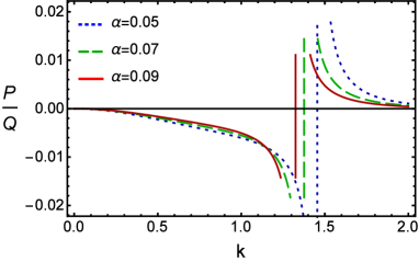
Figure 1: The variation of $P/Q$ with $k$ for different values of $\alpha$ when $\delta=1.2$, $\lambda=1.5$, $\kappa=2$, $\mu_{1}=0.7$, and $\mu_{2}=0.5$.

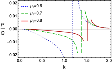
Figure 2: The variation of $P/Q$ with $k$ for different values of $\mu_{1}$ when $\alpha=0.07$, $\delta=1.2$, $\lambda=1.5$, $\kappa=2$, and $\mu_{2}=0.5$.

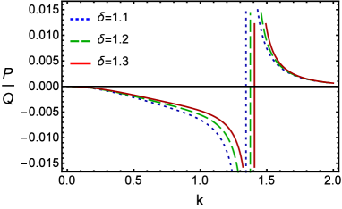
Figure 3: The variation of $P/Q$ with $k$ for different values of $\delta$ when $\alpha=0.07$, $\lambda=1.5$, $\kappa=2$, $\mu_{1}=0.7$, and $\mu_{2}=0.5$.

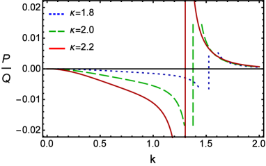
Figure 4: The variation of $P/Q$ with $k$ for different values of $\kappa$ when $\alpha=0.07$, $\delta=1.2$ $\lambda=1.5$, $\mu_{1}=0.7$, and $\mu_{2}=0.5$.

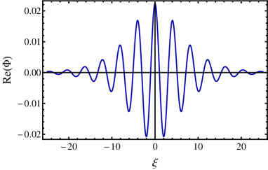
Figure 5: The bright envelope solitons for $\alpha=0.07$, $\delta=1.2$, $\lambda=1.5$, $\kappa=2$, $\mu_{1}=0.8$, $\mu_{2}=0.5$, $\tau=0$, $\psi_{0}=0.0005$, $U=0.2$, $\Omega_{0}=0.4$, and $k=1.6$.

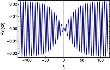
Figure 6: The dark envelope solitons for $\alpha=0.07$, $\delta=1.2$, $\lambda=1.5$, $\kappa=2$, $\mu_{1}=0.8$, $\mu_{2}=0.3$, $\tau=0$, $\psi_{0}=0.0005$, $U=0.2$, $\Omega_{0}=0.4$, and $k=1.2$.

4 Modulational instability

The stable and unstable parametric regimes of IAWs are organised by the sign of $P$ and $Q$ of Eq. (26) [23, 24, 25, 26, 27, 28, 29, 30]. When $P$ and $Q$ have the same sign (i.e., $P/Q>0$), the evolution of IAWs amplitude is modulationally unstable in the presence of external perturbations. On the other hand, when $P$ and $Q$ have opposite signs (i.e., $P/Q<0$), the IAWs are modulationally stable in the presence of external perturbations. The plot of $P/Q$ against $k$ yields stable and unstable parametric regimes of the IAWs. The point, at which the transition of $P/Q$ curve intersects with the $k$-axis, is known as the threshold or critical wave number $k~{}(=k_{c})$ [23, 24, 25, 26, 27, 28, 29, 30].

5 Envelope Solitons

The bright (when $P/Q>0$) and dark (when $P/Q<0$) envelope solitonic solutions, respectively, can be written as [23, 24]

$$\Phi(\xi,\tau)=\left[\psi_{0}~{}\mbox{sech}^{2}\left(\frac{\xi-U\tau}{W}\right)\right]^{\frac{1}{2}}$$

$$\times\exp\left[\frac{i}{2P}\left\{U\xi+\left(\Omega_{0}-\frac{U^{2}}{2}\right)\tau\right\}\right],$$ (29)

$$\Phi(\xi,\tau)=\left[\psi_{0}~{}\mbox{tanh}^{2}\left(\frac{\xi-U\tau}{W}\right)\right]^{\frac{1}{2}}$$

$$\times\exp\left[\frac{i}{2P}\left\{U\xi-\left(\frac{U^{2}}{2}-2PQ\psi_{0}\right)\tau\right\}\right],$$ (30)

where $\psi_{0}$ is the amplitude of localized pulse for both bright and dark envelope soliton, $U$ is the propagation speed of the localized pulse, $W$ is the soliton width, and $\Omega_{0}$ is the oscillating frequency at $U=0$. The soliton width $W$ and the maximum amplitude $\psi_{0}$ are related by $W=\sqrt{2\mid P/Q\mid/\psi_{0}}$. We have observed the bright and dark envelope solitons in Fig. 5-6.

6 Results and discussion

We have graphically examined the effects of the temperature of warm ion and super-thermal electron as well as the charge state of the warm ion in recognizing the stable and unstable domains of the IAWs in Fig. 1, and it is clear from this figure that (a) the stable domain decreases with the increase in the value of warm ion temperature but increases with the increase of the value of super-thermal electron temperature when the charge state of the warm ion remains constant; (b) the stable domain increases with $Z_{+}$ for constant value of $T_{+}$ and $T_{e1}$ (via $\alpha=3T_{+}/Z_{+}T_{e1}$). So, the charge state and temperature of warm ion play an opposite role in manifesting the stable and unstable domains of IAWs.

Both stable (i.e., $k<k_{c}$) and unstable (i.e., $k>k_{c}$) domains for the IAWs can be observed from Fig. 2, and it is obvious from this figure that (a) when $\mu_{1}=0.6$, $0.7$, and $0.8$, then the corresponding value of $k_{c}$ is $1.20$ (dotted blue curve), $1.40$ (dashed green curve), and $1.50$ (solid red curve); (b) $k_{c}$ is shifted to higher values with the increase (decrease) of $n_{e10}$ ($n_{+0}$) when the value of $Z_{+}$ is constant. Finally, $\mu_{1}$ would cause to increase the stable domain of IAWs;

We have numerically analyzed the effect of temperature of the super-thermal electron and super-thermal positron on the stability conditions of IAWs in Fig. 3. It can be seen from this figure that the stable domain increases with the increase (decrease) in the value of super-thermal electron (positron) temperature. Figure 4 describes the effects of super-thermality of plasma species in the stable and unstable parametric domains. It is clear from this figure that for large values of $\kappa$, the IAWs become unstable for small values of $k$ while for small values of $\kappa$, the IAWs become unstable for large values of $k$.

7 Conclusion

We have studied an unmagnetized realistic space plasma system consists of warm ions, iso-thermal electrons, $\kappa$-distributed electrons and positrons. The RPM is used to derive the NLSE. The existence of both stable and unstable regions of IAWs has been found, and the interaction between the $k_{c}$ with various plasma parameters (i.e., $\alpha$, $\mu_{1}$, $\delta$, and $\kappa$, etc.) has also been observed. Finally, these results may be applicable in understanding the conditions of the MI of IAWs and associated envelope solitons in astrophysical environments.

References

- [1] A. Panwar, et al., Phys. Plasmas 21 (2014) 122105.
- [2] I. Kourakis, et al., J. Phys. A Math. Gen. 36 (2003) 11901.
- [3] H. Alinejad, et al., Astrophys. Space Sci. 352 (2014) 571.
- [4] M.A. Rehman, et al., Phys. Plasmas 23 (2016) 012302.
- [5] M. Shahmansouri, et al., Phys. Plasmas 20 (2013) 082130.
- [6] Shalini, et al., Phys. Plasmas 22 (2015) 092124.
- [7] T.K. Baluku, et al., Phys. Plasmas 19 (2012) 012106.
- [8] T.K. Baluku, et al., J. Geophys. Res. 116 (2011) A04227.
- [9] R.E. Ergun, et al., Geophy. Res. Lett. 25 (1998) 2061.
- [10] M. Temerin, et al., Phys. Rev. Lett. 48 (1982) 1175.
- [11] N.A. Chowdhury, et al., Chaos 27 (2017) 093105.
- [12] N.A. Chowdhury, et al., Vacuum 147 (2018) 31.
- [13] E.C. Sittler, et al., J. Geophys. Res. 88 (1983) 8847.
- [14] D.T. Young, et al., Science 307 (2005) 1262.
- [15] R. Pottelette, et al., Geophys. Res. Lett. 26 (1999) 2629.
- [16] V.M. Vasyliunas, J. Geophys. Res. 73 (1968) 2839.
- [17] N.A. Chowdhury, et al., Contrib. Plasma Phys. 58 (2018) 870.
- [18] R.K. Shikha, et al., Eur. Phys. J. D 73 (2019) 177.
- [19] M. Hassan, et al., Commun. Theor. Phys. 71 (2019) 1017.
- [20] S.K. Paul, et al., Pramana-J Phys 94 (2020) 58.
- [21] T.I. Rajib, et al., Phys. plasmas 26 (2019) 123701.
- [22] N. Ahmed, et al., Chaos 28 (2018) 123107.
- [23] I. Kourakis, et al., Nonlinear Proc. Geophys. 12 (2005) 407.
- [24] S. Sultana, et al., Plasma Phys. Control. Fusion 53 (2011) 045003.
- [25] N.A. Chowdhury, et al., Phys. plasmas 24 (2017) 113701.
- [26] M.H. Rahman, et al., Phys. Plasmas 25 (2018) 102118.
- [27] S. Jahan, et al., Commun. Theor. Phys. 71 (2019) 327.
- [28] S. Jahan, et al., Plasma Phys. Rep. 46 (2020) 90.
- [29] N.A. Chowdhury, et al., Plasma Phys. Rep. 45 (2019) 459.
- [30] M.H. Rahman, et al., Chinese J. Phys. 56 (2018) 2061.