A General Automatic Method for Optimal Construction of Matrix Product Operators Using Bipartite Graph Theory

Abstract

Constructing matrix product operators (MPO) is at the core of the modern density matrix renormalization group (DMRG) and its time dependent formulation. For DMRG to be conveniently used in different problems described by different Hamiltonians, in this work we propose a new generic algorithm to construct the MPO of an arbitrary operator with a sum-of-products form based on the bipartite graph theory. We show that the method has the following advantages: (i) It is automatic in that only the definition of the operator is required; (ii) It is symbolic thus free of any numerical error; (iii) The complementary operator technique can be fully employed so that the resulting MPO is globally optimal for any given order of degrees of freedom; (iv) The symmetry of the system could be fully employed to reduce the dimension of MPO. To demonstrate the effectiveness of the new algorithm, the MPOs of Hamiltonians ranging from the prototypical spin-boson model and Holstein model to the more complicated ab initio electronic Hamiltonian and the anharmonic vibrational Hamiltonian with sextic force field are constructed. It is found that for the former three cases, our automatic algorithm can reproduce exactly the same MPOs as the optimally hand-crafted ones already known in the literature.

I Introduction

The density matrix renormalization group (DMRG) method originally proposed by White to solve the electronic structure of one-dimensional strongly correlated lattice models White (1992) has made great progress in quantum chemistry in the last decade and has been widely recognized as a state-of-the-art method for problems with a large active space. Chan and Sharma (2011); Ren, Yi, and Shuai (2016); Ma et al. (2017); Yanai et al. (2017); Li and Chan (2017); Luo et al. (2018); Baiardi and Reiher (2020); Brandejs et al. (2020) In addition to the electronic correlation, DMRG also shows great potential to solve the vibrational correlated problems. Rakhuba and Oseledets (2016); Baiardi et al. (2017, 2019) More recently, the time dependent (TD) formulation of DMRG called TD-DMRG attracts a lot of attention and quickly emerges as an efficient and “nearly exact” method for quantum dynamics in complex systems. TD-DMRG has been used to simulate the spectroscopy and quantum dynamics, including not only electron dynamics Ronca et al. (2017); Frahm and Pfannkuche (2019) but also electron-vibrational correlated dynamics. Greene and Batista (2017); Yao et al. (2018); Ren, Shuai, and Kin-Lic Chan (2018); Kurashige (2018); Baiardi and Reiher (2019); Xie et al. (2019); Li, Ren, and Shuai (2020a, b) For high-dimensional quantum dynamics, the multi-configuration time-dependent Hartree (MCTDH) method has long been considered as the gold standard. Meyer, Manthe, and Cederbaum (1990); Beck et al. (2000) However, it is limited by the exponential growth of computational cost with the system size – the curse of dimensionality. The multilayer MCTDH (ML-MCTDH) overcomes this limitation and has been successfully applied to simulate dynamics of model systems with thousands of degrees of freedom (DoF). Wang and Thoss (2003) Like ML-MCTDH, (TD-)DMRG could also achieve arbitrarily high accuracy with only polynomial computational effort. It has been demonstrated in a number of models with hundreds of DoFs to have the same accuracy as ML-MCTDH. Ren, Shuai, and Kin-Lic Chan (2018); Xie et al. (2019); Yao et al. (2018); Kurashige (2018); Larsson (2019)

The recent rapid advances in quantum chemistry DMRG can be attributed to the formulation of DMRG as matrix product state (MPS) Östlund and Rommer (1995) and the corresponding operator could be represented as matrix product operator (MPO). Crosswhite and Bacon (2008) The introduction of MPS and MPO not only establishes a rigorous mathematical foundation of DMRG, but also makes the algorithm more powerful and convenient. Schollwöck (2011) Furthermore, it also opens the door to the development of more general tensor network states (TNS) such as tree tensor network states (TTNS) Nakatani and Chan (2013); Gunst et al. (2018) and projected entangled pair states (PEPS). Li, O’Rourke, and Chan (2019) DMRG is actually a special type of TNS with an one-dimensional matrix product ansatz, which is mathematically known as a tensor train (TT) format. Interestingly, from the TNS point of view, ML-MCTDH has a TTNS wavefunction ansatz with all physical DoF (primitive basis) at the leaf-node (lowest layer), which is mathematically called hierarchical Tucker format. In this sense, the ansatz of DMRG and ML-MCTDH are both low-rank approximations to the exact high-rank wavefunction, although historically they are independently developed in different research fields White (1992); Meyer, Manthe, and Cederbaum (1990); Wang and Thoss (2003). The modern formulation of the DMRG algorithm based on MPS and MPO is usually called the second generation DMRG algorithm, Keller et al. (2015) which could be seamlessly combined with the variational principle to obtain the ground state and the time dependent variational principle to carry out the time propagation. Haegeman et al. (2016); Li, Ren, and Shuai (2020a) In addition, the exact global arithmetic, such as additions $\Psi_{1}+\Psi_{2},\hat{O}_{1}+\hat{O}_{2}$ and multiplications $\hat{O}\Psi,\hat{O}_{1}\hat{O}_{2}$, are only possible based on MPS and MPO. In this new formulation, the starting point is to construct the MPO representation of the Hamiltonian and all the other required operators as an input to the rest DMRG calculations.

Generally speaking, there are two different types of operators. One is the analytical operators, such as the ab initio electronic Hamiltonian in quantum chemistry, the nuclear kinetic energy operator in an appropriate set of coordinates and most of the physical and chemical model Hamiltonians. In addition, these analytical operators are commonly in a sum-of-products (SOP) form. The other type is the potential energy operator of real molecules met in molecular nuclear Schrödinger equation. More specifically, the potential energy “operator” here is a complex $N$-dimensional potential energy surface (PES) $V(\bm{q})=V(q_{1},q_{2},\cdots q_{N})$ and has no analytical forms. The potential energy (or energy derivative) at a specific structure $\bm{q}$ could be calculated by electronic structure calculation. For small-sized molecules with several atoms, very high accurate PESs are usually constructed globally by fitting and interpolating the available dataset of ab initio data points. The recent developed algorithm based on the neural network (NN) has made great progress in the direction. Raff et al. (2012); Jiang and Guo (2013) For medium- and large-sized molecules, constructing full-dimensional global PESs is not even possible. The local PES around the equilibrium or saddle point could be expanded as a Taylor series with the high order energy derivatives. Though the Taylor expansion of PES has several known limitations such as that it could not describe double well potential and large amplitude motion, it is still very useful to calculate the anharmonic frequency of semi-rigid molecules and obtain a more accurate IR/Raman spectrum beyond the harmonic approximation. Barone, Biczysko, and Bloino (2014); Barone (2005); Barone et al. (2012) For most numerical methods to solve the nuclear Schrödinger equation such as (ML-)MCTDH, one difficulty is to calculate the matrix element such as $\langle\Psi|V(\bm{q})|\Psi\rangle$, which is an $N$-dimensional quadrature problem. To reduce the cost, it is preferred to decompose the potential into an SOP form. In this way, the matrix elements could be calculated as a sum of product of $N$ one-dimensional quadrature. The Taylor series expansion of the local potential apparently has an SOP form. For a general PES, Potfit Jäckle and Meyer (1996) and the more efficient multigrid Potfit method Peláez and Meyer (2013) could decompose the PES numerically into a Tucker format from the energy grid points, which is suitable to the MCTDH calculation. The recently developed multilayer Potfit could integrate more effectively with ML-MCTDH. Otto (2014) Besides the Potfit-like methods, in the NN algorithm to fit the PES, if the activation function is an exponential function instead of the common hyperbolic tangent or sigmoid function, the NN with a single hidden layer also gives an analytical SOP form. Manzhos and Carrington Jr (2006) In addition to the SOP form, one of the other widely used methods to overcome the $N$-dimensional quadrature is called $n$-mode representation ($n$-MR), in which the PES is expanded as a sum of one-mode potential, two-mode potential and so on, expecting that the series could converge with a small number of terms. Carter, Culik, and Bowman (1997) Thus, only low dimensional quadrature is needed. If necessary, each term in $n$-MR could be further fitted as a sum of products of analytical functions such as polynomial and Morse types for each individual mode. Klinting et al. (2018) It is also worth mentioning that several methods could directly use the $N$-dimensional PES, like the MCTDH combined with correlation discrete variable (CDVR) representation Manthe (1996) and its multilayer generalization Manthe (2008) proposed by Manthe and the collocation method proposed by Carrington et al. Avila and Carrington Jr (2013)

In this work, we focus on the construction of MPO for those operators that have an SOP form by definition or have been transformed into an SOP form by fitting a high-dimensional function (discrete points) as introduced above. For the same operator, the form of MPO could be completely different as long as the final product is correct. However, a more compact MPO will save computational cost in practice. In order to construct a compact MPO, several methods have been proposed. The most commonly used method in quantum chemistry is to design MPO symbolically (or sometimes called analytically) by hand through inspecting the recurrence relation between neighboring sites. Chan et al. (2016) The so-called complementary operator technique is always fully explored to make the MPO more compact, which is essential to the operators with long-range interactions, Xiang (1996) such as the ab initio electronic Hamiltonian. Though usually this method could give the optimal answer by a smart design, it is not automatic in that different operators need a re-design and a re-implementation. The second one is a numerically “top-down” algorithm in which a naive MPO is first constructed and then compressed by the singular value decomposition (SVD) or by removing the linearly dependent terms. Hubig, McCulloch, and Schollwöck (2017) This algorithm is generic and automatic for different operators, while a numerical error is introduced and its effect on the following calculations cannot be well quantified in advance. Apart from this, the time cost spent on the numerical compression is not negligible when the number of terms in the operator is large. The third one which is not widely used in quantum chemistry is to construct a finite-state automaton to mimic the interaction terms in the operator. Crosswhite and Bacon (2008) The automaton is easy to be constructed for a translationally invariant lattice model with short-range interactions, but becomes extremely complicated for long-range interactions.

Unlike the ab-initio electronic Hamiltonian which has the same formula for different systems and thus could be hard-coded in implementation, a general Hamiltonian could be completely different according to the different interactions within the system. Thus, it is not efficient to use the first hand-crafting method mentioned above to construct MPOs on a case-by-case basis. In addition to the inefficiency, it is also difficult to obtain a globally optimal MPO when the Hamiltonian is very complicated. Therefore, it is necessary and desired to have a better MPO construction algorithm which has all the advantages of the methods introduced above: (i) It is generic for all types of operators with an analytical SOP form; (ii) It is automatic, directly from the symbolic operator strings to the MPO; (iii) It gives an optimal MPO. Here, “optimal” means that the MPO is as compact as possible globally in a given order of DoF; (iv) It is symbolic thus free of any numerical error. In this work, we propose a new MPO construction algorithm which meets all the four requirements based on the graph theory for a bipartite graph. The remaining sections of this paper are arranged as follows. In section II, we will present the idea of the new algorithm and the implementation details. In section III, several typical Hamiltonians are examined ranging from the simple spin-boson model and Holstein model to the more complicated ab initio electronic Hamiltonian and vibrational Hamiltonian described by a sextic force field. All the calculations are carried out with our in-house code Renormalizer. ren The resulting MPOs are compared with the optimally hand-crafted ones reported in the literature.

II Methodology and Implementation

II.1 MPO and complementary operator technique

The wavefunction ansatz in DMRG is called the matrix product states or tensor train, which is

$$|\Psi\rangle=\sum_{\{a\},\{\sigma\}}A[1]^{\sigma_{1}}_{a_{1}}A[2]^{\sigma_{2}}_{a_{1}a_{2}}\cdots A[N]^{\sigma_{N}}_{a_{N-1}}|\sigma_{1}\sigma_{2}\cdots\sigma_{N}\rangle.$$ (1)

For a system of distinguishable particles, $N$ is the number of DoFs in the system and $\{|\sigma_{i}\rangle\}$ is the local basis such as the discrete variable representation (DVR) basis for nuclear motion. For electronic systems, $N$ is the number of orbitals and $\{|\sigma_{i}\rangle\}$ is the occupation configuration of each orbital (if using spatial-orbital, $\{|\sigma_{i}\rangle\}=\{|\textrm{vacuum}\rangle,|\uparrow\rangle,|\downarrow\rangle,|\uparrow\downarrow\rangle\}$; if using spin-orbital, $\{|\sigma_{i}\rangle\}=\{|\textrm{vacuum}\rangle,|\textrm{occupied}\rangle\}$.). $\{A[i]^{\sigma_{i}}_{a_{i-1}a_{i}}\}$ are the local matrices connected by the indices $a_{i}$, which is commonly called (virtual) bond with bond dimension $M_{\textrm{S}}$ or denoted as $|a_{i}|$. $\sigma_{i}$ is called the physical bond with dimension $d$. One good feature of DMRG is that the accuracy is only determined by the dimension of the virtual bond, and thus could be systematically improved.

Similar to MPS, any operator $\hat{O}$ could be expressed as a matrix product operator: Schollwöck (2011); Chan et al. (2016)

$$\hat{O}=\sum_{\{w\},\{\sigma\},\{\sigma^{\prime}\}}W[1]^{\sigma^{\prime}_{1},\sigma_{1}}_{w_{1}}W[2]^{\sigma^{\prime}_{2},\sigma_{2}}_{w_{1}w_{2}}\cdots W[N]^{\sigma^{\prime}_{N},\sigma_{N}}_{w_{N-1}}|\sigma^{\prime}_{1}\sigma^{\prime}_{2}\cdots\sigma^{\prime}_{N}\rangle\langle\sigma_{N}\sigma_{N-1}\cdots\sigma_{1}|.$$ (2)

MPO could be constructed by sequential singular value decompositions from the matrix element representation $\mathbf{O}_{\sigma_{1}^{\prime}\sigma_{2}^{\prime}\cdots\sigma_{N}^{\prime},\sigma_{1}\sigma_{2}\cdots\sigma_{N}}$ numerically, but it is not practical for a large system since the exact decomposition needs the bond dimension $M_{O}$ to increase exponentially, which is $d^{2},d^{4},\cdots,d^{N-2},d^{N},d^{N-2},\cdots,d^{2}$ if $N$ is even. In practice, if an operator has an SOP form, MPO is usually first constructed symbolically,

$$\hat{O} =\sum_{\{z\}}\gamma_{z_{1}z_{2}\cdots z_{N}}\hat{z}_{1}\hat{z}_{2}\cdots\hat{z}_{N}$$ (3)

$$=\sum_{\{w\},\{z\}}W[1]^{z_{1}}_{w_{1}}W[2]^{z_{2}}_{w_{1}w_{2}}\cdots W[N]^{z_{N}}_{w_{N-1}}\hat{z}_{1}\hat{z}_{2}\cdots\hat{z}_{N}$$ (4)

$$=\sum_{\{w\}}\hat{W}[1]_{w_{1}}\hat{W}[2]_{w_{1}w_{2}}\cdots\hat{W}[N]_{w_{N-1}}.$$ (5)

In Eq. (3), $\{\hat{z}_{i}\}$ represents the elementary operators of each local site such as $\{\hat{I},\hat{p}^{2},\hat{x},\hat{x}^{2},f(\hat{x},\hat{p}),\textrm{etc}\}$ for a vibrational site or $\{\hat{I},\hat{a}^{\dagger},\hat{a},\hat{a}^{\dagger}\hat{a}\}$ for an electronic site. The prefactor $\gamma_{z_{1}z_{2}\cdots z_{N}}$ is commonly very sparse. For example, in the ab initio electronic Hamiltonian, $\gamma_{z_{1}z_{2}\cdots z_{N}}=0$ if more than four $\hat{z}_{i}$ are $\hat{a}^{\dagger}$ or $\hat{a}$. $\gamma_{z_{1}z_{2}\cdots z_{N}}$ could be regarded as the coefficient of $\hat{O}$ on the operator basis $\hat{z}_{1}\hat{z}_{2}\cdots\hat{z}_{N}$ and its matrix product representation in Eq. (4) is very similar to an MPS in Eq. (1). In Eq. (5), $\hat{W}[i]=\sum_{z_{i}}W[i]^{z_{i}}\hat{z}_{i}$ is a matrix composed of some prefactor attached symbolic operators acting locally on site $i$. From this symbolic MPO, it is easy to obtain the matrix element representation as Eq. (2) by expanding $\hat{W}[i]$ on the local basis $\{|\sigma_{i}\rangle\}$.

From $\gamma_{z_{1}z_{2}\cdots z_{N}}$, if all terms with a nonzero prefactor are extracted, $\hat{O}$ can also be expressed as

$$\hat{O}=\sum_{o=1}^{K}\hat{O}[1:N]_{o}=\sum_{o=1}^{K}(\gamma_{o}\prod_{i=1}^{N}\hat{z}_{i}^{o}).$$ (6)

$K$ is the number of nonzero terms in total. $\hat{z}_{i}^{o}$ is the local operator of the $o$th term at site $i$ and could be any of the elementary operators in $\hat{z}_{i}$. The slice $[1:N]$ indicates that the operator is from site $1$ to site $N$. The MPO representation of each term $\hat{O}[1:N]_{o}$ in Eq. (6) has $M_{O}=1$ with $\hat{W}[i]=\hat{z}_{i}^{o}$ and the prefactor $\gamma_{o}$ could be attached to any site. The global arithmetic addition of any two MPOs (not necessary to have $M_{O}=1$) is

$$\gamma_{1}\hat{O}[1:N]_{1}+\gamma_{2}\hat{O}[1:N]_{2}=\begin{bmatrix}\hat{z}_{1}^{1}&\hat{z}_{1}^{2}\end{bmatrix}\big{(}\prod_{i=2}^{N-1}\begin{bmatrix}\hat{z}_{i}^{1}&\mathbf{0}\\ \mathbf{0}&\hat{z}_{i}^{2}\end{bmatrix}\big{)}\begin{bmatrix}\gamma_{1}\hat{z}_{N}^{1}\\ \gamma_{2}\hat{z}_{N}^{2}\end{bmatrix},$$ (7)

which merges the local matrices block-diagonally. Therefore, the naive way to construct MPO of $\hat{O}$ in Eq. (6) will give $M_{O}=K$.

A more systematic way to derive MPO is to use the recurrence relation between the neighboring sites. When the system is split between site $i$ and site $i+1$ into the respective left (L, from site 1 to $i$) and right (R, from site $i+1$ to $N$) blocks, $\hat{O}$ could be expressed as

$$\hat{O}=\sum_{o_{i}=1}^{K}\gamma_{o_{i}}\cdot\hat{O}[1:i]_{o_{i}}\otimes\hat{O}[i+1:N]_{o_{i}}$$ (8)

$\hat{O}[1:i]_{o_{i}}=\prod_{j=1}^{i}\hat{z}_{j}^{o_{i}}$ and $\hat{O}[i+1:N]_{o_{i}}=\prod_{j=i+1}^{N}\hat{z}_{j}^{o_{i}}$ are usually called the normal operators. A recurrence relation between the neighboring $\hat{O}[1:i-1]_{o_{i-1}}$ and $\hat{O}[1:i]_{o_{i}}$ could be defined as

$$\hat{O}[1:i]_{o_{i}}=\sum_{o_{i-1}=1}^{K}\hat{O}[1:i-1]_{o_{i-1}}\hat{O}[i]_{o_{i-1}o_{i}},$$ (9)

from which the symbolic MPO in Eq. (5) could be obtained directly with $\hat{W}[i]=\hat{O}[i]$ and again the prefactor $\gamma_{o_{i}}$ could be attached to any site. This construction gives the same result as the global arithmetic addition of $K$ MPOs with $M_{O}=1$ in Eq. (7). However, it is apparently not optimal in that some of the interaction terms in Eq. (8) may share the common operators in the set $\{\hat{O}[1:i]_{o_{i}}\}$ or $\{\hat{O}[i+1:N]_{o_{i}}\}$. For example, if $K=2$ and $\hat{O}[i+1:N]_{1}\equiv\hat{O}[i+1:N]_{2}$ while $\hat{O}[1:i]_{1}\neq\hat{O}[1:i]_{2}$, $\hat{O}[1:i]_{1}$ and $\hat{O}[1:i]_{2}$ could be summed up with the prefactors to create a complementary operator $\hat{\tilde{O}}[1:i]_{1}=\gamma_{1}\hat{O}[1:i]_{1}+\gamma_{2}\hat{O}[1:i]_{2}$ on the L-block and meanwhile $\hat{O}[i+1:N]_{2}$ is removed from the R-block so that $\hat{O}=\hat{\tilde{O}}[1:i]_{1}\otimes\hat{O}[i+1:N]_{1}$. Thus, $|o_{i}|$, the number of columns of $\hat{O}[i]$, is reduced by 1. This example shows that the MPO representation of the same operator is not unique as long as the product result is correct. Generally speaking, to make the MPO compact, if there are redundant operators in $\{\hat{O}[i+1:N]_{o_{i}}\}$($\{\hat{O}[1:i]_{o_{i}}\}$), the corresponding left (right) complementary operators could be created. This complementary operator technique Xiang (1996) is of essential importance in constructing MPO for ab initio electronic Hamiltonian by assembling all the 4-index operators $\sum_{pqrs}g_{pqrs}a^{\dagger}_{p}a^{\dagger}_{q}a_{r}a_{s}$ and 3-index operators $\sum_{pqr}g_{pqrs}a^{\dagger}_{p}a^{\dagger}_{q}a_{r}$ and part of the 2-index operators in one block, reducing $M_{O}$ from $\mathcal{O}(N^{4})$ to $\mathcal{O}(N^{2})$. Keller et al. (2015); Chan et al. (2016) However, the complexity of designing complementary operators comes from that in most Hamiltonian both $\hat{O}[1:i]_{o_{i}}$ and $\hat{O}[i+1:N]_{o_{i}}$ in one interaction term are correlated to other interaction terms. For instance, we add another two terms in the former example, $\hat{O}[1:i]_{1}\equiv\hat{O}[1:i]_{3}$ and $\hat{O}[1:i]_{2}\equiv\hat{O}[1:i]_{4}$. In this case, the optimal solution is to create complementary operators $\hat{\tilde{O}}[i+1:N]_{1}=\gamma_{1}\hat{O}[i+1:N]_{1}+\gamma_{3}\hat{O}[i+1:N]_{3}$ and $\hat{\tilde{O}}[i+1:N]_{2}=\gamma_{2}\hat{O}[i+1:N]_{2}+\gamma_{4}\hat{O}[i+1:N]_{4}$, which will give $|o_{i}|=2$. While creating the complementary operator $\hat{\tilde{O}}[1:i]_{1}$ as above will result in $|o_{i}|=3$. This toy example shows that the design of complementary operators is nontrivial. A typical real example is that when constructing MPO of the ab initio electronic Hamiltonian, a different design strategy of the complementary operators of the 2-index operators within one block will lead to a different $M_{O}$ shown in Figure 10 of Ref. 49 though all of them are $\mathcal{O}(N^{2})$. Therefore, the key to construct a compact MPO is to design and select the normal and complementary operators smartly at each bond to make the number of retained operators as small as possible. As far as we know, up to now it is still an art to design the complementary operators by hand on a case-by-case basis rather than by a rigorous and automatic procedure.

II.2 MPO construction algorithm via bipartite graph theory

We propose to use the theory of bipartite graph to set a rigorous foundation to construct MPO automatically. We first reinterpret the operator selection problem at each bond mentioned in section II.1 as a minimum vertex cover problem in a bipartite graph and then prove that the locally optimal solution is also globally optimal.

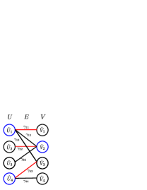
Figure 1: An example of mapping the operator $\hat{O}=\gamma_{11}\hat{U}_{1}\hat{V}_{1}+\gamma_{12}\hat{U}_{1}\hat{V}_{2}+\gamma_{13}\hat{U}_{1}\hat{V}_{3}+\gamma_{22}\hat{U}_{2}\hat{V}_{2}+\gamma_{32}\hat{U}_{3}\hat{V}_{2}+\gamma_{43}\hat{U}_{4}\hat{V}_{3}+\gamma_{44}\hat{U}_{4}\hat{V}_{4}$ to a bipartite graph $G=(U,V,E)$. The vertices represent the non-redundant operators in the L- and R- block. The edges represent the interactions with a nonzero prefactor. The vertices in blue form a minimum vertex cover. The edges in red form a maximum matching.

The non-redundant operator set by removing the duplicated operators in $\{\hat{O}[1:i]_{o_{i}}\},\{\hat{O}[i+1:N]_{o_{i}}\}$ of Eq. (8) are denoted as $U=\{\hat{U}[1:i]_{u_{i}}\},V=\{\hat{V}[i+1:N]_{v_{i}}\}$, which are represented as the vertices in Fig. 1. Unlike that the interaction pattern is one-to-one between $\{\hat{O}[1:i]_{o_{i}}\}$ and $\{\hat{O}[i+1:N]_{o_{i}}\}$, it would be one-to-many between $\{\hat{U}[1:i]_{u_{i}}\}$ and $\{\hat{V}[i+1:N]_{v_{i}}\}$. The $K$ interaction terms are represented as the edges denoted as $E$ each connecting one vertex in $U$ to one vertex in $V$ with a prefactor (weight) $\gamma_{u_{i}v_{i}}$. A bipartite graph is often denoted as $G=(U,V,E)$. If the $p$th vertex in $U$ is selected, the corresponding operator $\hat{U}[1:i]_{p}$ in the L-block is retained. Meanwhile, the operators $\hat{V}[i+1:N]_{q}$ corresponding to the vertices in $V$ which are linked to $\hat{U}[1:i]_{p}$ through edges are multiplied by the prefactor of the certain edge and then are added up to create a new complementary operator in the R-block $\sum_{q}\gamma_{pq}\hat{V}[i+1:N]_{q}$. The same rule is applied if a vertex in $V$ is selected. Therefore, the minimal number of retained operators in one block which could cover all the $K$ interaction terms is equal to the minimal number of selected vertices in $(U,V)$ which could cover all the edges in $E$ (shown in blue in Fig. 1). The latter problem is called the minimum vertex cover in graph theory. For a bipartite graph described here, König theorem proves that the number of vertices in the minimum vertex cover is equal to the number of edges in the maximum matching. Bondy, Murty et al. (1976) A matching is an edge set in which any two edges do not share one vertex. The maximum matching shown in red in Fig. 1 is the matching having the maximal number of edges, which could be solved efficiently by the Hungarian algorithm Kuhn (1955) with complexity $\mathcal{O}(nm)$ or the Hopcroft–Karp algorithm Hopcroft and Karp (1973) with complexity $\mathcal{O}(\sqrt{n}m)$ through finding an augmenting path. Bondy, Murty et al. (1976) Here, $n$ and $m$ are the total number of vertices and edges in the bipartite graph. Once the maximum matching is found, the vertices in the minimum vertex cover could be obtained easily and the retained operators are optimally selected according to the rules above.

For a DMRG chain with a certain order, the whole procedure to construct the MPO of $\hat{O}$ from site $1$ to $N$ (from $N$ to $1$ is similar) is summarized as follows.

1. The incoming non-redundant operator set of site $i$ is known as $\{\hat{W}[1:i-1]_{w_{i-1}}\}$ ($\{\hat{W}[1:0]\}$ is $\{1\}$), which are also the outgoing operators of site $i-1$. Commonly, $\{\hat{W}[1:i-1]_{w_{i-1}}\}$ includes both normal operators and complementary operators. Next, $\{\hat{W}[1:i-1]_{w_{i-1}}\}$ is multiplied by the local elementary operators $\{\hat{z}_{i}\}$ on site $i$ to form a non-redundant operator set $\{\hat{U}[1:i]_{u_{i}}\}=\{\hat{W}[1:i-1]_{w_{i-1}}\}\otimes\{\hat{z}_{i}\}$. The R-block non-redundant operator set is $\{\hat{V}[i+1:N]_{v_{i}}\}$, in which all operators are normal operators. Note that for efficiency only the interaction terms with a nonzero prefactor are necessary to be included in the operator sets $\{\hat{U}[1:i]_{u_{i}}\}$ and $\{\hat{V}[i+1:N]_{v_{i}}\}$. Hence, at this boundary between site $i$ and $i+1$, $\hat{O}=\sum_{u_{i}v_{i}}\gamma_{u_{i}v_{i}}\hat{U}[1:i]_{u_{i}}\otimes\hat{V}[i+1:N]_{v_{i}}$.

2. The operators in $\{\hat{U}[1:i]_{u_{i}}\}$, $\{\hat{V}[i+1:N]_{v_{i}}\}$ and the interactions between them are represented as vertices and edges to form a bipartite graph $G=(U,V,E)$ (see Fig. 1). Afterward, the maximum matching and the corresponding minimum vertex cover of this bipartite graph is found with the Hungarian algorithm or the Hopcroft–Karp algorithm. Next, iterating through each vertex in the minimum vertex cover once:

   1. If the vertex is the $p$th vertex in $U$, the operator $\hat{U}[1:i]_{p}$ is retained and meanwhile the edges linked to it are removed from the graph.

   2. If the vertex is the $q$th vertex in $V$, the complementary operator linked through edges to $\hat{V}[i+1:N]_{q}$ is created and retained, which is $\hat{\tilde{U}}[1:i]_{q}=\sum_{p}\gamma_{pq}\hat{U}[1:i]_{p}$. Meanwhile, the edges are removed.

   The reason to remove the edges after each visit is to avoid the double-counting of the interactions. After all the vertices in the minimum vertex cover are visited once, there will be no edge in the graph.

3. The retained operators $\hat{U}[1:i]_{p}$ and $\hat{\tilde{U}}[1:i]_{q}$ together form a new non-redundant operator set $\{\hat{W}[1:i]_{w_{i}}\}$ in the L-block. It is the outgoing operator set of site $i$ and meanwhile is the incoming operator set of site $i+1$. After that, with $\{\hat{W}[1:i-1]_{w_{i-1}}\}$ and $\{\hat{W}[1:i]_{w_{i}}\}$, the local symbolic MPO $\hat{W}[i]$ is easy to obtain according to the recurrence relation $\hat{W}[1:i]=\hat{W}[1:i-1]\hat{W}[i]$. In fact, the local prefactor matrix $W[i]^{z_{i}}_{w_{i-1}w_{i}}$ in $\hat{W}[i]_{w_{i-1}w_{i}}=\sum_{z_{i}}W[i]^{z_{i}}_{w_{i-1}w_{i}}\hat{z}_{i}$ is the transformation matrix (reshaped to be $W[i]_{w_{i-1}z_{i},w_{i}}$) of operator basis from $\{\hat{W}[1:i-1]_{w_{i-1}}\}\otimes\{\hat{z}_{i}\}$ to $\{\hat{W}[1:i]_{w_{i}}\}$.

   Return back to step 1..

The procedure described above is apparently a locally optimal solution, since the selected operators have already been the minimum vertex cover at each boundary when sweeping from the left to the right. To prove that the locally optimal solution is also globally optimal, we should prove that at each boundary between site $i$ and $i+1$, the number of edges in the maximum matching (the number of vertices in the minimum vertex cover) is the same no matter whether the operator set of L-block is composed of all normal operators or is composed of both normal operators and complementary operator as $\{\hat{W}[1:i]_{w_{i}}\}$ according to step 1. to step 3.. Following Eq. (3), if the coefficient tensor $\gamma_{z_{1}z_{2}\cdots z_{N}}$ is reshaped as a matrix $\gamma_{i}=\gamma_{z_{1}z_{2}\cdots z_{i},z_{i+1}\cdots z_{N}}$, it could be regarded as the coefficient matrix of $\hat{O}$ expanded on the operator basis $\{\hat{z}_{1}\otimes\cdots\otimes\hat{z}_{i}\}\otimes\{\hat{z}_{i+1}\otimes\cdots\otimes\hat{z}_{N}\}$ in the operator space. $\gamma_{i}$ is called the unfolding matrix of $\gamma$ in Ref. 56, whose rank is denoted as $r_{i}$ called TT-rank. The bipartite graph $G[i]=(U[i],V[i],E[i])$ at the boundary between site $i$ and site $i+1$ is $U[i]=\{\hat{z}_{1}\otimes\cdots\otimes\hat{z}_{i}\}$, $V[i]=\{\hat{z}_{i+1}\otimes\cdots\otimes\hat{z}_{N}\}$, the edges $E[i]$ has a one-to-one correspondence to the nonzero matrix elements in $\gamma_{i}$. In the bipartite graph theory, the matrix $\gamma_{i}$ could also be regarded as a symbolic bipartite adjacency matrix, for which only that the matrix elements are zero or nonzero is important. Lovász proposed the theorem that the rank of the symbolic adjacency matrix is equal to the number of edges of a maximum matching. Lovász (1979) Therefore, since $U[i]$ and $V[i]$ are composed of all normal operators, using the rules described above to select the normal and complementary operators, the ideally minimal number of retained operators at this boundary is equal to $r_{i}$, the rank of matrix $\gamma_{i}$. In Appendix A, we prove that sweeping from left to right as the procedure above will not change the rank of the adjacency matrix at the same boundary. It is worth noting that in Ref. 51, the ideal rank $r_{i}$ of MPO at the $i$th bond is expected to be approached by numerical SVD compression, deparallelization and delinearization, but it is not guaranteed because of the numerical error. But here, it is guaranteed symbolically via the bipartite graph theory. In addition, the scaling of the current algorithm is roughly $\mathcal{O}(K^{3/2}N)$ with Hopcroft–Karp algorithm. In comparison, The scaling of the SVD-based algorithm is roughly $\mathcal{O}(K^{3}d^{2}N)$. Thus, the current algorithm is much cheaper.

Several other advantages of the algorithm are that (i) The sparsity of MPO is fully maintained, which could be used to reduce the computational cost during the tensor contraction in DMRG single state or time evolution algorithms. (ii) The symmetry could be directly implemented by attaching the good quantum numbers on each normal and complementary operator. (iii) The algorithm not only works for MPO construction, but also works for MPS construction if the wavefunction in the Fock space representation has already been known. For the same reason, the obtained MPS is the most compact one to represent the wavefunction exactly.

Finally, it should be mentioned that for a system in which the interaction pattern is inhomogeneous, the order of DoFs will affect the size of MPO. It is still unclear whether there is an algorithm which could efficiently find out a specific order giving the minimal MPO. However, in our opinion, this problem is less of a priority than the widely known ordering problem with respect to the accuracy of DMRG calculation. Legeza and Sólyom (2003); Moritz, Hess, and Reiher (2005)

III Results

In this section, we will demonstrate the effectiveness of the new algorithm by constructing the MPOs of Hamiltonians ranging from the simple spin-boson model and Holstein model to the more complicated ab initio electronic Hamiltonian and vibrational Hamiltonian with a sextic force field.

III.1 Spin-boson model and Holstein model

The spin-boson model (expressed in the first quantization formalism in Eq. (10)) describes a two-level system coupled with a harmonic bath, which is widely used to investigate the quantum dissipation.

$$\hat{H}_{\textrm{SBM}}=\epsilon\hat{\sigma}_{z}+\Delta\hat{\sigma}_{x}+\frac{1}{2}\sum_{i}(\hat{p}_{i}^{2}+\omega^{2}_{i}\hat{q}_{i}^{2})+\hat{\sigma}_{z}\sum_{i}c_{i}\hat{q}_{i}$$ (10)

Holstein model (expressed in the second quantization formalism in Eq. (11)) is also a widely used electron-vibrational coupling model to describe the charge transport, energy transfer and spectroscopy of molecular aggregates. Schröter et al. (2015); Ren, Shuai, and Kin-Lic Chan (2018); Li, Ren, and Shuai (2020a); Jiang et al. (2020); Li, Ren, and Shuai (2020b) It could be regarded as a group of two-level systems as the spin-boson model coupled with each other through coupling constant $J_{ij}$.

$$\hat{H}_{\textrm{Holstein}}=\sum_{i}\varepsilon_{i}a_{i}^{\dagger}a_{i}+\sum_{i\neq j}J_{ij}a_{i}^{\dagger}a_{j}+\sum_{in}\omega_{in}b_{in}^{\dagger}b_{in}+\sum_{in}\omega_{in}g_{in}a_{i}^{\dagger}a_{i}(b_{in}^{\dagger}+b_{in})$$ (11)

Both of the two models are often adopted to benchmark the quantum dynamics methods. We put the two models in the same section because spin-boson model could be regarded as a one-site Holstein model with an additional interstate coupling $\Delta$ and thus the MPOs of them are very similar. We test a spin-boson model with 100 discrete modes and the order is $[\textrm{spin},v_{1},v_{2}\cdots,v_{100}]$. We also test two Holstein models with 20 electronic sites and both of them have two vibrational modes of each electronic site but the former only has one-dimensional nearest-neighbor electronic hopping while the latter has long-range hoppings between any two electronic sites. The order of the Holstein model is $[e_{1},v_{1,1},v_{1,2},e_{2},v_{2,1},v_{2,2},\cdots,e_{20},v_{20,1},v_{20,2}]$. The MPO bond dimension $M_{O}$ versus the bond index is shown in Fig. 2. The reference results (blue line) are based on a hand-crafted strategy, in which the normal operators for the electronic coupling terms are switched to the complementary operators $\hat{P}_{j}=\sum_{i}J_{ij}a_{i}$ and $\hat{P}_{j}^{\dagger}=\sum_{i}J_{ij}a^{\dagger}_{i}$ after passing the middle electronic site. The details are provided in the appendix in our former work, Ren, Shuai, and Kin-Lic Chan (2018) which is believed to be near-optimal for the two models (from the results shown below, it is optimal except at the first bond for the Holstein model.).

For the spin-boson model shown in Fig. 2a, $M_{O}$ is a constant independent of system size because $\hat{W}[1:i]=\{\hat{H}[1:i],\hat{\sigma}_{z},\hat{I}\}$ where $\hat{H}[1:i]$ is the complete Hamiltonian from site 1 to $i$. The new automatic algorithm gives exactly the same result as the hand-crafted one. For the Holstein model shown in Fig. 2b and  2c, $M_{O}$ is independent of the number of the electronic site when the electronic coupling is one-dimensional nearest-neighbor coupling, while it is linearly dependent on the number of the electronic site if the long-range hopping is allowed. The new automatic algorithm gives the same results as the hand-crafted ones except at the first bond, where the new algorithm gives one less bond dimension. This minor difference comes from that the hand-crafted strategy gives $\hat{W}[1]=\{\varepsilon_{1}a_{1}^{\dagger}a_{1},a^{\dagger}_{1}a_{1},a^{\dagger}_{1},a_{1},\hat{I}\}$ while the automatic algorithm gives $\hat{W}[1]=\{a^{\dagger}_{1}a_{1},a^{\dagger}_{1},a_{1},\hat{I}\}$ and the local energy of the first site $\varepsilon_{1}a^{\dagger}_{1}a$ is considered in $\hat{W}[2]_{0,0}=\varepsilon_{1}\hat{I}$. Though this small improvement will not make a noticeable difference on the actual computational cost, it is clear to demonstrate that since the new algorithm is globally optimal, it could find out the redundancy which will be neglected sometimes with the common hand-crafted strategy.

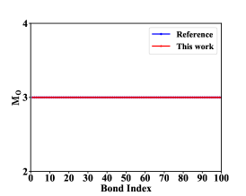
(a)

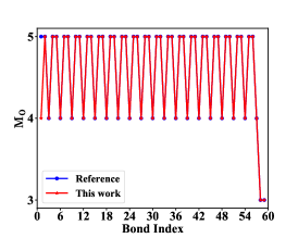
(b)

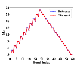
(c)

Figure 2: The bond dimension $M_{O}$ versus the bond index in (a) spin-boson model with 100 discrete vibrational modes. (b) Holstein model of 20 electronic sites with only one-dimensional electronic coupling and each electronic site has two vibrational modes. (c) same as (b) except with arbitrary long-range electronic couplings. The reference results (blue line) are based on the hand-crafted complementary operator strategy provided in our former work. Ren, Shuai, and Kin-Lic Chan (2018)

III.2 Ab initio electronic Hamiltonian

The second Hamiltonian considered is the ab initio electronic Hamiltonian, in which up to 4 sites interact with each other. Thus it is much more complicated than the spin-boson model and Holstein model. With spin-orbitals, the Hamiltonian is written as

$$\hat{H}_{\textrm{el}}=\sum_{p,q=1}^{N}h_{pq}a_{p}^{\dagger}a_{q}+\frac{1}{2}\sum_{p,q,r,s=1}^{N}v_{pqrs}a_{p}^{\dagger}a_{q}^{\dagger}a_{r}a_{s}=\sum_{p,q=1}^{N}h_{pq}a_{p}^{\dagger}a_{q}+\sum_{p<q,r<s}^{N}g_{pqrs}a_{p}^{\dagger}a_{q}^{\dagger}a_{r}a_{s}$$ (12)

where the two-electron integral $v_{pqrs}$ is $(ps|qr)$ in chemist’s notation. The second equality takes advantage of the symmetry in $v_{pqrs}$ ($g_{pqrs}=v_{pqrs}-v_{qprs}=v_{pqrs}-v_{pqsr}$).

Firstly, we introduce the optimal hand-crafted strategy to construct the MPO of ab initio electronic Hamiltonian. For more implementation details, please refer to Ref. 49. For convenience, $\hat{H}_{\textrm{el}}$ is divided into three components. The first part is $\hat{H}_{1}=\hat{H}_{L}+\hat{H}_{R}$, in which $\hat{H}_{L}$ and $\hat{H}_{R}$ are respectively the full Hamiltonian of the orbitals in the L-block and R-block. In fact, $\hat{H}_{L}$ and $\hat{H}_{R}$ could be regarded as the complementary operators of identity operator $\hat{I}_{R}$ and $\hat{I}_{L}$ in the R-block and L-block, reducing $\mathcal{O}(N^{4})$ normal operators to 1 complementary operator. Apparently, $\hat{H}_{1}$ gives $M_{O,1}=2$ at each bond. The second part with two fermionic creation or annihilation (elementary) operators in each block is written as

$$\hat{H}_{2}=\sum_{p<q,r<s} -g_{p_{L}q_{R}r_{L}s_{R}}\left(a_{p_{L}}^{\dagger}a_{r_{L}}\right)\left(a_{q_{R}}^{\dagger}a_{s_{R}}\right)$$

$$+g_{p_{L}q_{L}r_{R}s_{R}}\left(a_{p_{L}}^{\dagger}a_{q_{L}}^{\dagger}\right)\big{(}a_{r_{R}}a_{s_{R}}\big{)}$$

$$+g_{p_{R}q_{R}r_{L}s_{L}}\big{(}a_{r_{L}}a_{s_{L}}\big{)}\left(a_{p_{R}}^{\dagger}a_{q_{R}}^{\dagger}\right)$$ (13)

The optimal strategy to design the complementary operator depends on the number of orbitals denoted as $n_{L}$ and $n_{R}$ in each block. For instance, if $n_{L}>n_{R}$, the complementary operators of the first term in Eq. (13) is $\hat{P}_{qs}=\sum_{pr}-g_{p_{L}q_{R}r_{L}s_{R}}\left(a_{p_{L}}^{\dagger}a_{r_{L}}\right)$, which have $n_{R}^{2}$ terms in total. Therefore, the ideally minimal bond dimension is $M_{O,2}=\min(n_{L}^{2},n_{R}^{2})+2\cdot\min(n_{L}(n_{L}-1)/2,n_{R}(n_{R}-1)/2)$. The third part with one creation or annihilation operator in one block and three in the other is commonly written as

$$\hat{H}_{3}= \sum_{p}a_{p_{L}}^{\dagger}\left(\sum_{q}\frac{1}{2}h_{p_{L}q_{R}}a_{q_{R}}+\sum_{qrs}g_{p_{L}q_{R}r_{R}s_{R}}a_{q_{R}}^{\dagger}a_{r_{R}}a_{s_{R}}\right)$$

$$+\sum_{r}a_{r_{L}}\left(\sum_{s}-\frac{1}{2}h_{s_{R}r_{L}}a_{s_{R}}^{\dagger}+\sum_{pqs}g_{p_{R}q_{R}r_{L}s_{R}}a_{p_{R}}^{\dagger}a_{q_{R}}^{\dagger}a_{s_{R}}\right)$$

$$+\sum_{q}\left(\sum_{p}-\frac{1}{2}h_{q_{R}p_{L}}a_{p_{L}}+\sum_{psr}g_{p_{L}q_{R}r_{L}s_{L}}a_{p_{L}}^{\dagger}a_{r_{L}}a_{s_{L}}\right)a_{q_{R}}^{\dagger}$$

$$+\sum_{s}\left(\sum_{r}\frac{1}{2}h_{r_{L}s_{R}}a_{r_{L}}^{\dagger}+\sum_{pqr}g_{p_{L}q_{L}r_{L}s_{R}}a_{p_{L}}^{\dagger}a_{q_{L}}^{\dagger}a_{r_{L}}\right)a_{s_{R}}$$ (14)

The terms in the parentheses are the complementary operators which should be firstly summed up. This kind of complementary operators is adopted to construct MPO of ab initio electronic Hamiltonian, because it greatly reduces $M_{O,3}$ from $\mathcal{O}(N^{3})$ to $\mathcal{O}(N)$. However, it is only near-optimal because near the left boundary of the chain, there are more 1-index operators in the R-block than 3-index operators in the L-block. Thus, the optimal way to construct the complementary operator at this boundary is

$$\hat{H}_{3}= \sum_{p}a_{p_{L}}^{\dagger}\left(\sum_{q}h_{p_{L}q_{R}}a_{q_{R}}+\sum_{qrs}g_{p_{L}q_{R}r_{R}s_{R}}a_{q_{R}}^{\dagger}a_{r_{R}}a_{s_{R}}\right)$$

$$+\sum_{r}a_{r_{L}}\left(\sum_{s}-h_{s_{R}r_{L}}a_{s_{R}}^{\dagger}+\sum_{pqs}g_{p_{R}q_{R}r_{L}s_{R}}a_{p_{R}}^{\dagger}a_{q_{R}}^{\dagger}a_{s_{R}}\right)$$

$$+\sum_{prs}a_{p_{L}}^{\dagger}a_{r_{L}}a_{s_{L}}\left(\sum_{q}g_{p_{L}q_{R}r_{L}s_{L}}a_{q_{R}}^{\dagger}\right)$$

$$+\sum_{pqr}a_{p_{L}}^{\dagger}a_{q_{L}}^{\dagger}a_{r_{L}}\left(\sum_{s}g_{p_{L}q_{L}r_{L}s_{R}}a_{s_{R}}\right)$$ (15)

The case is the same near the right boundary of the chain. Therefore, the minimal $M_{O,3}$ equals $2\cdot\min(n_{L}^{2}(n_{L}-1)/2,n_{R})+2\cdot\min(n_{L},n_{R}^{2}(n_{R}-1)/2)$. It is clear that $M_{O,2}$ contributes most to the total $M_{O}=M_{O,1}+M_{O,2}+M_{O,3}$, and thus this improvement of $M_{O,3}$ is rarely considered. But it could be considered automatically with our new algorithm. Adding up the contributions of the three components, the largest bond dimension always lies in the middle of the chain, which is $M_{O,\textrm{max}}=2(\frac{N}{2})^{2}+3(\frac{N}{2})+2$.

To consider the antisymmetry of fermions in the algorithm described in section  II.2, the Jordan-Wigner transformation Jordan and Wigner (1928) for the elementary creation and annihilation operators is introduced. Keller et al. (2015); Li and Chan (2017)

$$|\textrm{vacuum}\rangle=|\alpha\rangle$$ (16)

$$|\textrm{occupied}\rangle=|\beta\rangle$$ (17)

$$a^{\dagger}_{j}=\prod_{i=1}^{j-1}\sigma_{z}[i]\times\sigma_{-}[j]$$ (18)

$$a_{j}=\prod_{i=1}^{j-1}\sigma_{z}[i]\times\sigma_{+}[j]$$ (19)

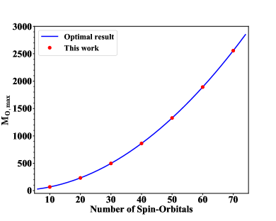
(a)

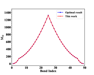
(b)

Figure 3: (a) The maximal MPO bond dimension $M_{O,\textrm{max}}$ of ab initio electronic Hamiltonian with different number of spin-orbitals. The blue curve $M_{O,\textrm{max}}=2(\frac{N}{2})^{2}+3(\frac{N}{2})+2$ is the optimal result from the hand-crafted complementary operator strategy (see text for details). The red circles are the results obtained from the new automatic MPO construction algorithm. (b) The MPO bond dimension $M_{O}$ at each bond of ab initio electronic Hamiltonian of a 50 spin-orbitals system.

Fig. 3a shows the maximal $M_{O}$ of systems with 10 to 70 spin-orbitals and Fig. 3b shows $M_{O}$ at each bond of a system with 50 spin-orbitals. The correctness of the MPOs generated by the automatic algorithm has been verified by checking the residue $\|\textrm{MPO}_{1}-\textrm{MPO}_{2}\|=0$ with respect to the MPOs developed by Li et al. in Ref. 6 and implemented in package QCMPO. QCM $M_{O}$ at each bond and $M_{O,\textrm{max}}$ (red asterisks) of the automatically generated MPO exactly match what the optimally hand-crafted strategy described above would give (blue circles), except that at the first bond the automatic algorithm gives $M_{O}=4$ ($\hat{W}[1]=[\sigma_{-}\sigma_{+},\sigma_{z}\sigma_{-},\sigma_{z}\sigma_{+},\hat{I}]$) while the hand-crafted strategy gives $M_{O}=5$ ($\hat{W}[1]=[h_{11}\sigma_{-}\sigma_{+},\sigma_{-}\sigma_{+},\sigma_{z}\sigma_{-},\sigma_{z}\sigma_{+},\hat{I}]$). The reason is the same as that in the case of Holstein models. In addition, in Fig. 3b, $M_{O}$ versus the bond index is symmetric as expected and the kink at the bond index 5 and 45 is due to the switch of the complementary operators from Eq. (15) to Eq. (14), indicating that the new algorithm could really find out the optimal solution.

We also calculate the ground state energy of water molecule with 6-31g basis by the MPO-based DMRG algorithm. The structure of H₂O in the Cartesian coordinates is $\textrm{O}(0,0,-0.0644484)$, $\textrm{H}(\pm 0.7499151,0,0.5114913)$ in Angstroms. The electron integral and the reference full configuration interaction (FCI) result are calculated by PySCF. Sun et al. (2018) The DMRG results with different $M_{S}$ are shown in Fig. 4. The error of ground state energy with $M_{S}=800$ is less than $1\times 10^{-6}\,E_{\textrm{h}}$, which verifies the correctness of the MPO generated by the automatic algorithm.

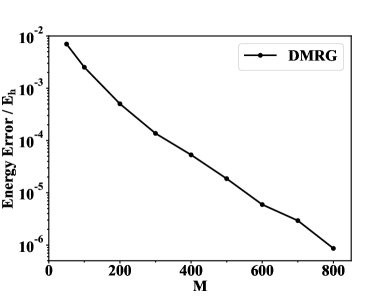
Figure 4: The error of the ground state energy of H₂O with 6-31g basis calculated by MPO based DMRG algorithm with different MPS bond dimension $M_{S}$. The two-site algorithm is adopted to optimize the ground state MPS. The reference is the FCI energy $E_{\textrm{FCI}}=-76.11969704\,E_{\textrm{h}}$. The MPO is generated by the new automatic MPO construction algorithm.

III.3 Anharmonic vibrational Hamiltonian

The third example considered is the anharmonic vibrational Hamiltonian. There are two difficulties to solve the vibrational problems. One is how to calculate the matrix elements of high-dimensional PES as introduced in the first section. The other is how to calculate the eigenstates or simulate the dynamics. Both of these two difficulties stem from the curse of dimensionality. To overcome the second difficulty, there have been a series of methods at different hierarchical levels including vibrational self consistent field (VSCF), vibrational perturbation theory (VPT), vibrational configuration interaction (VCI), vibrational coupled cluster (VCC) and multi-reference approaches. Barone (2005); Christiansen and Luis (2005); Christiansen (2012); Qu and Bowman (2019); Mizukami and Tew (2013); Pfeiffer and Rauhut (2014) (ML-)MCTDH combined with the improved relaxation algorithm Doriol et al. (2008) is another efficient method to obtain the eigenstates of vibrational Hamiltonian. Recently, DMRG has also been proposed to solve the anharmonic vibrational problem. Rakhuba and Oseledets (2016); Baiardi et al. (2017, 2019) Herein we use an approximate form of the Watson Hamiltonian, in which only the second-order Coriolis terms are included, Carbonniere and Barone (2004); Baiardi et al. (2017); Sibaev and Crittenden (2016)

$$\hat{H}=\hat{H}_{\textrm{vib}}+\hat{H}_{\textrm{Cor}}$$ (20)

$$\hat{H}_{\textrm{vib}}=-\frac{1}{2}\sum_{i}\frac{\partial^{2}}{\partial q_{i}^{2}}+V(\{\bm{q}\})$$ (21)

$$\hat{H}_{\textrm{Cor}}=-\sum_{\alpha}B_{\alpha}\sum_{i<j}\sum_{k<l}\zeta_{ij}^{\alpha}\zeta_{kl}^{\alpha}\left(q_{i}\frac{\partial}{\partial q_{j}}-q_{j}\frac{\partial}{\partial q_{i}}\right)\left(q_{k}\frac{\partial}{\partial q_{l}}-q_{l}\frac{\partial}{\partial q_{k}}\right)$$ (22)

$B_{\alpha}$ are the rotational constants and $\zeta_{ij}^{\alpha}$ the Coriolis coupling constants. In this numerical example, $V(\{\bm{q}\})$ is approximated as a sixth order Taylor expansion around the equilibrium geometry.

$$V(\{\bm{q}\})=V_{0}+\frac{1}{2}\sum_{i}\omega_{i}^{2}q_{i}^{2}+\frac{1}{3!}\sum_{ijk}F_{ijk}q_{i}q_{j}q_{k}+\frac{1}{4!}\sum_{ijkl}F_{ijkl}q_{i}q_{j}q_{k}q_{l}$$

$$+\frac{1}{5!}\sum_{ijklm}F_{ijklm}q_{i}q_{j}q_{k}q_{l}q_{m}+\frac{1}{6!}\sum_{ijklmn}F_{ijklmn}q_{i}q_{j}q_{k}q_{l}q_{m}q_{n}$$ (23)

It is a nontrivial task to construct a compact MPO of the operator in Eq.(23), because up to six sites are coupled together in a DMRG chain, more complicated than the ab initio electronic Hamiltonian. We note that two methods have been used to construct MPO of this type of operators. In Ref. 10 a compact MPO is constructed by SVD compression and in Ref. 11 a symbolic MPO is constructed in the second quantization formalism as the electronic Hamiltonian. Keller et al. (2015) We will use the automatic MPO construction algorithm to demonstrate its effectiveness and generality. Though we use a PES expanded as a Taylor series in this example, it is worth mentioning that the algorithm is suitable to any PES expressed as an analytical SOP form. The molecule we choose is the widely studied C₂H₄ molecule Baiardi et al. (2017, 2019); Christiansen and Luis (2005); Sibaev and Crittenden (2015, 2016). The PES of C₂H₄ used here is a sextic force field as Eq. (23) from PyPES library, Sibaev and Crittenden (2015) which is an adaptation of the PES constructed at CCSD(T) level with quadruple-zeta basis in internal coordinates. Delahaye et al. (2014) The constant $V_{0}$ is set to 0 for simplicity. Since C₂H₄ at equilibrium geometry has D_2h point group symmetry, there are only 2644 nonzero potential energy terms in the Hamiltonian otherwise it would be 18485 terms.

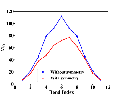
Figure 5: The MPO bond dimension $M_{O}$ versus bond index of C₂H₄ described by a sextic force field with or without considering D_2h point group symmetry.

Fig. 5 shows the MPO bond dimension at each bond of $\hat{H}_{\textrm{vib}}$ of C₂H₄ with or without considering the point group symmetry. The 12 vibrational DoFs within the DMRG chain are arranged according to their harmonic frequencies $\omega_{i}$. With point group symmetry, the largest MPO bond dimension is reduced from 112 to 77, which will reduce the computational cost spent in the DMRG static state or the time evolution calculations. Because the construction is automatic, the gain by utilizing symmetry to reduce the size of MPO is for free. Therefore, for Hamiltonian with negligible terms, it would be efficient to use the current algorithm to construct MPO after pre-screening the prefactors.

We use the linear response DMRG method under the Tamm-Dancoff approximation (DMRG-TDA) to calculate the vibrational excited states. Wouters et al. (2013); Nakatani et al. (2014) Compared to the other DMRG based algorithms for the high-lying excited states, such as DMRG with shift-and-invert scheme Dorando, Hachmann, and Chan (2007); Yu, Pekker, and Clark (2017); Baiardi et al. (2019), DMRG with the folded operator Baiardi et al. (2019) and DMRG with projector and energy-shift Baiardi et al. (2017); Larsson (2019), DMRG-TDA has the advantage that all the required eigenstates could be calculated in a single calculation and there is no need to track a specific state during the DMRG optimization procedure in order to avoid the root flipping problem. Hu and Chan (2015); Baiardi et al. (2019) To the best of our knowledge, it is the first time that DMRG-TDA is applied to the vibrational correlation problem. In our calculation, the maximal occupation number (quanta) of each mode is limited to 6. The ground state is calculated by state-averaged DMRG (SA-DMRG) for the lowest 9 states to make the renormalized basis more balanced for not only the ground state itself but also the excited states. Based on this ground state, we use DMRG-TDA to calculate all the eigenstates below 4000 cm^-1. In Table 1, we list the zero point energy, all 12 fundamental bands and the combination bands below 4000 cm^-1 composed of a high-frequency C-H stretch and a low-frequency bend motion. The energy levels with or without considering the Coriolis coupling are both listed. Each DMRG-TDA wavefunction is compressed to a rank one Hartree product state to assign the main configuration in the correlated wavefunction. The label of each normal mode follows Ref. 74 and is listed in Table S1 of the supplementary material. For comparison, the VCI(8) results calculated by the PyVCI package  Sibaev and Crittenden (2016) and the variational results reported in the literature  Delahaye et al. (2014) are also listed. Table 1 shows that the DMRG-TDA results have already converged within $1\,\textrm{cm}^{-1}$ with only $M_{S}=50$ for the fundamental bands. For the combination bands listed, the convergence within $1\,\textrm{cm}^{-1}$ could be reached with $M_{S}=100$ except the energy level $v_{1}+v_{8}$ ($<1.5\,\textrm{cm}^{-1}$). One of the reasons for this difference is that DMRG-TDA is a single site excitation method on a correlated ground state reference. Thus, it is more efficient to target the fundamental bands than the combination bands. More sophisticated DMRG-CISD method Wouters et al. (2013), in which the second-order tangent space of MPS is also included, could further improve the accuracy of the combination bands. All the energy levels below 4000 cm^-1 are listed in Table S2 in the supplementary material. The root mean square deviation of the DMRG-TDA results ($M_{S}=200$) including the effect of Coriolis coupling compared to the available theoretical data in Ref. 74 is $0.74\,\textrm{cm}^{-1}$ for the fundamental bands and $9.12\,\textrm{cm}^{-1}$ for all bands below 4000 cm^-1. We expect that if the same form of PES is used, the deviation would be smaller. Though we choose a small molecule C₂H₄ as a numerical example here, VDMRG is suitable for much larger molecules, such as that in Ref. 11 a peptide molecule is calculated.

Table 1: The zero point energy (ZPE), twelve fundamental frequencies and eight stretch-bend combination frequencies below 4000 cm^-1 of C₂H₄ calculated by DMRG-TDA.

assignment	without Coriolis term					with Coriolis term
	harmonic	DMRG-TDA			VCI(8) a	DMRG-TDA			VCI(8) a	Ref. 74
		$M_{S}=50$	$M_{S}=100$	$M_{S}=200$		$M_{S}=50$	$M_{S}=100$	$M_{S}=200$
ZPE	11164.45	11011.62	11011.62	11011.62	11011.63	11017.10	11016.95	11016.95	11016.96	11014.91
$v_{10}$	824.97	820.25	820.01	819.99	820.11	823.69	823.55	823.53	823.66	822.42
$v_{8}$	950.19	926.68	926.35	926.33	926.45	935.43	935.21	935.18	935.31	934.29
$v_{7}$	966.39	942.03	941.68	941.65	941.78	950.89	950.64	950.61	950.74	949.51
$v_{4}$	1050.81	1017.81	1017.48	1017.45	1017.56	1026.05	1025.83	1025.80	1025.92	1024.94
$v_{6}$	1246.76	1222.41	1222.17	1222.15	1222.23	1224.91	1224.81	1224.79	1224.87	1225.41
$v_{3}$	1369.38	1342.26	1341.97	1341.95	1342.01	1342.94	1342.80	1342.79	1342.85	1342.46
$v_{12}$	1478.48	1438.61	1438.33	1438.31	1438.39	1441.90	1441.77	1441.76	1441.84	1441.11
$v_{2}$	1672.57	1623.23	1622.93	1622.90	1622.97	1625.51	1625.37	1625.34	1625.41	1624.43
$v_{11}$	3140.91	2978.69	2978.09	2978.01	2978.20	2985.73	2985.35	2985.28	2985.48	2985.38
$v_{1}$	3156.84	3017.93	3017.17	3017.06	3017.05	3020.17	3019.20	3019.07	3019.15	3018.99
$v_{5}$	3222.89	3072.75	3071.86	3071.20	3071.51	3079.63	3079.27	3079.17	3079.36	3079.86
$v_{9}$	3248.71	3092.41	3091.58	3091.39	3091.98	3101.40	3101.14	3101.07	3101.26	3101.69
$v_{11}+v_{10}$		3792.91	3790.82	3790.53	3791.73	3805.76	3804.14	3803.85	3805.05	3803.51
$v_{1}+v_{10}$		3831.52	3828.88	3828.57	3829.80	3836.10	3834.30	3834.02	3835.17	3833.27
$v_{5}+v_{10}$		3889.77	3886.71	3885.77	3887.13	3899.93	3897.17	3896.77	3897.92
$v_{11}+v_{8}$		3902.58	3897.06	3897.02	3897.86	3926.18	3914.00	3914.03	3914.74	3912.73
$v_{9}+v_{10}$		3910.79	3909.17	3908.85	3910.21	3922.38	3921.02	3920.79	3921.83	3921.08
$v_{11}+v_{7}$		3917.10	3911.44	3911.39	3912.24	3936.35	3929.24	3929.22	3930.05	3927.84
$v_{1}+v_{8}$		3936.71	3937.59	3936.20	3931.12	3952.56	3943.27	3942.03	3944.20	3946.68
$v_{5}+v_{8}$		3974.11	3969.67	3970.02	3970.30	4006.88	4000.06	4000.43	4000.66

^a the VCI(8) results are calculated by Package PyVCI from Ref. 73; 72. VCI(8) means that up to 8 quanta could be excited in the CI calculation $\sum_{i}^{N}n_{i}\leq 8$ ($n_{i}$ is the number of quanta of the $i$th mode).

Finally, we briefly discuss the computational scaling when using the MPO based DMRG algorithms. When dealing with the ab initio electronic Hamiltonian, it has been pointed out that directly treating the MPO as a dense matrix will result in an incorrect scaling $\mathcal{O}(N^{5})$ compared to $\mathcal{O}(N^{4})$ of the original DMRG algorithm in which only the renormalized operator matrix is retained. Keller et al. (2015); Chan et al. (2016) The same problem will arises for the vibrational Hamiltonian with sextic force field. The $M_{O,\textrm{max}}$ of $\hat{H}_{\textrm{vib}}$ with the number of vibrational modes is shown in Fig. 6 (blue curve). For $\hat{H}_{\textrm{vib}}$, $M_{O,\textrm{max}}=\frac{1}{48}N^{3}+\frac{3}{8}N^{2}+\frac{5}{3}N+2$ when $N$ is even. The leading term $\mathcal{O}(N^{3})$ comes from the 3-index normal operators in each block and the prefactor is $\binom{N/2}{3}$. When calculating the expectation value $\langle\Psi|\hat{H}|\Psi\rangle$ or optimizing the ground state, the cost spent in each blocking process is $\mathcal{O}(N^{6})$, because the size of each local matrix in MPO is $\mathcal{O}(N^{3})\times\mathcal{O}(N^{3})$. Hence, the total cost after each sweep is $\mathcal{O}(N^{7})$. However, with the original DMRG algorithm, the bottleneck in the blocking process is to contract the 3-index normal operators $q_{i}q_{j}q_{k}$ in the L-block (R-block) and 1-index operator $q_{l}$ in the center site to the complementary operator of $q_{m}q_{n}$ in the R-block (L-block), which is $\hat{P}_{mn}=\sum_{ijk}F_{ijklmn}q_{i}q_{j}q_{k}q_{l}$, with a local computational scaling $\mathcal{O}(N^{5})$ and in total $\mathcal{O}(N^{6})$ in one sweep. To recover the correct scaling in the MPO based algorithm, two approaches have been proposed. One is to fully employ the sparsity of MPO when contracting tensors. Keller et al. (2015) The other method is to split the total $\hat{H}_{\textrm{vib}}$ into a sum of $\hat{H}_{i}$, Li and Chan (2017); Chan et al. (2016) $\hat{H}_{\textrm{vib}}=\sum_{i=1}^{N}\hat{H}_{i}$, where

$$\hat{H}_{i}=-\frac{1}{2}\frac{\partial^{2}}{\partial q_{i}^{2}}+V_{0}/N+\frac{1}{2}\omega_{i}^{2}q_{i}^{2}+\frac{1}{3!}\sum_{jk}F_{ijk}q_{i}q_{j}q_{k}+\frac{1}{4!}\sum_{jkl}F_{ijkl}q_{i}q_{j}q_{k}q_{l}$$

$$+\frac{1}{5!}\sum_{jklm}F_{ijklm}q_{i}q_{j}q_{k}q_{l}q_{m}+\frac{1}{6!}\sum_{jklmn}F_{ijklmn}q_{i}q_{j}q_{k}q_{l}q_{m}q_{n}.$$ (24)

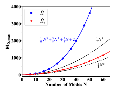
Figure 6: The maximal MPO bond dimension $M_{O,\textrm{max}}$ of the vibrational Hamiltonian $\hat{H}_{\textrm{vib}}$ in Eq. (21) (blue circle) and $\hat{H}_{i}$ in Eq. (24) (red star) versus the number of modes. The blue curve $\frac{1}{48}N^{3}+\frac{3}{8}N^{2}+\frac{5}{3}N+2$ exactly fits the $M_{O,\textrm{max}}$ of $\hat{H}_{\textrm{vib}}$. The two black dashed curves $\frac{1}{4}N^{2}$ and $\frac{1}{2}N^{2}$ indicate the scaling of $M_{O,\textrm{max}}$ of $\hat{H}_{i}$ is $\mathcal{O}(N^{2})$ and the prefactor is between $\frac{1}{4}$ and $\frac{1}{2}$.

For $\hat{H}_{i}$ with index $i$ fixed, the maximal 5-free-index operator will give an MPO with $M_{O,\textrm{max}}=\mathcal{O}(N^{2})$. The red curve in Fig. 6 shows $M_{O,\textrm{max}}$ of $\hat{H}_{i}$ with the number of modes. The prefactor of the leading term is between $\frac{1}{4}$ and $\frac{1}{2}$. If all the $N$ sub-MPOs are added up according to Eq. (7), the total MPO of $\hat{H}_{\textrm{vib}}$ will be recovered with the same scaling of the bond dimension $\mathcal{O}(N^{3})$ but with a larger prefactor. The advantage to introduce $\hat{H}_{i}$ is that the contraction of $\hat{H}$ could be first divided into contractions of $\hat{H}_{i}$ and then are summed up together. Even though the MPO of $\hat{H}_{i}$ is treated as a dense matrix, the computational scaling in the blocking process is $\mathcal{O}(N^{4})$ for each of them and the total $N$ MPOs will result in $\mathcal{O}(N^{5})$. Therefore, this “sum of MPO” algorithm not only recovers the correct computational scaling but also is easy to be parallelized.

IV Conclusion and Outlook

In this work, we propose a new generic algorithm for the construction of matrix product operator of any operator with an analytical sum-of-products form based on the bipartite graph theory. The most important feature of the algorithm is that it could translate the operator expression to the MPO representation automatically. Therefore, it is very useful for the current (TD-)DMRG methods to be easily extended to more problems described by different Hamiltonians. The idea of the new algorithm is to map the complementary operator selection problem to a minimum vertex cover problem in a bipartite graph, which could be elegantly solved by several well-established algorithms to get a locally optimal solution. We also prove that the constructed MPO is globally optimal. In addition, the new algorithm is symbolic and the sparsity of the Hamiltonian is fully preserved, which could be utilized to reduce the computational cost when contracting the tensors. We demonstrate the generality of the new algorithm by constructing MPOs ranging from the simple spin-boson model, Holstein model to the more complicated ab initio electronic Hamiltonian, and vibrational Hamiltonian described by a sextic force field. In all of the examples, the new algorithm performs well in that it could find out the small redundancy in the near-optimal hand-crafted MPO and it could take advantage of the symmetry to reduce the dimension of MPO. Finally, one potential use-case of the presented algorithm not covered in the former examples is that if the coordinates system in the vibrational problem is curvilinear coordinates instead of normal mode rectilinear coordinates, the nuclear kinetic energy operators could be very complicated. The polyspherical approach developed by Gatti and co-workers, Gatti and Iung (2009); Ndong et al. (2012) provides a general and analytical form of the kinetic energy operators expressed in terms of curvilinear coordinates, which often have thousands of summands and are very sensitive to numerical errors due to singularities. We expect that the symbolic feature of the current algorithm may be useful to contract the kinetic energy operators in these cases to reduce the computational cost when calculating the matrix elements.

supplementary material

See the supplementary material for the label of each normal mode of C₂H₄ and the energy levels below 4000 cm^-1 calculated by DMRG-TDA.

DATA AVAILABILITY

The data that support the findings of this study are available from the corresponding author upon reasonable request.

Appendix A Proof of the global optimality

We will prove that sweeping from left to right with the procedure described in section II.2 will not change the rank of the adjacency matrix at the same boundary. Starting from the left at the boundary between site $1$ and $2$, after the first loop through step 1. to step 3., the coefficient matrix $\gamma_{1}$ is factorized as

$$\gamma_{1}=\gamma_{z_{1},z_{2}\cdots z_{N}}=\sum_{w_{1}}W[1]_{z_{1},w_{1}}C[2:N]_{w_{1},z_{2}z_{3}\cdots z_{N}}$$ (25)

The matrix $W[1]_{z_{1},w_{1}}$ is the transformation matrix given in step 3.. According to Lovász’s theorem, the dimension of $w_{1}$, $|w_{1}|$, is equal to $r_{1}$. Eq. (25) is nothing but a special rank decomposition of matrix $\gamma_{1}$. Hence, both $W[1]$ (columns are linearly independent) and $C[2:N]$ (rows are linearly independent) have rank $r_{1}$. Thus,

$$C[2:N]_{w_{1},z_{2}z_{3}\cdots z_{N}}=(W[1]^{T}W[1])^{-1}W[1]^{T}\gamma_{1}=X[1]\gamma_{1}$$ (26)

We will show that the unfolding matrices of $C[2:N]$, which are $C[2:N]_{2}=C[2:N]_{w_{1}z_{2},z_{3}\cdots z_{N}}$, $C[2:N]_{3}=C[2:N]_{w_{1}z_{2}z_{3},z_{4}\cdots z_{N}}$,$\cdots$, $C[2:N]_{N-1}=C[2:N]_{w_{1}z_{2}\cdots z_{N-1},z_{N}}$ all have $\textrm{rank}(C[2:N]_{i})=r_{i}$. Since $\gamma_{i}$ has rank $r_{i}$, a rank decomposition exists

$$\gamma_{i}=\gamma_{z_{1}\cdots z_{i},z_{i+1}\cdots z_{N}}=\sum_{\beta=1}^{r_{i}}H_{z_{1}\cdots z_{i},\beta}F_{\beta,z_{i+1}\cdots z_{N}}$$ (27)

Thus,

$$C[2:N]_{i} =C[2:N]_{w_{1}z_{2}\cdots z_{i},z_{i+1}\cdots z_{N}}$$

$$=\sum_{z_{1}}X[1]_{w_{1}z_{1}}\gamma_{z_{1}z_{2}\cdots z_{i},z_{i+1}\cdots z_{N}}$$

$$=\sum_{z_{1}}X[1]_{w_{1}z_{1}}\big{(}\sum_{\beta=1}^{r_{i}}H_{z_{1}\cdots z_{i},\beta}F_{\beta,z_{i+1}\cdots z_{N}}\big{)}$$

$$=\sum_{\beta=1}^{r_{i}}\big{(}\sum_{z_{1}}X[1]_{w_{1}z_{1}}H_{z_{1}\cdots z_{i},\beta}\big{)}F_{\beta,z_{i+1}\cdots z_{N}}$$

$$=\sum_{\beta=1}^{r_{i}}M_{w_{1}z_{2}\cdots z_{i},\beta}F_{\beta,z_{i+1}\cdots z_{N}}$$ (28)

Therefore, $\textrm{rank}(C[2:N]_{i})\leq r_{i}$. On the other hand, if $\textrm{rank}(C[2:N]_{i})<r_{i}$,

$$\gamma_{i} =\sum_{w_{1}}W[1]_{z_{1},w_{1}}C[2:N]_{w_{1},z_{2}z_{3}\cdots z_{N}}$$

$$=\sum_{w_{1}}W[1]_{z_{1},w_{1}}\big{(}\sum_{\beta=1}^{\textrm{rank}(C[2:N]_{i})}M^{\prime}_{w_{1}z_{2}\cdots z_{i},\beta}F^{\prime}_{\beta,z_{i+1}\cdots z_{N}}\big{)}$$

$$=\sum_{\beta=1}^{\textrm{rank}(C[2:N]_{i})}\big{(}\sum_{w_{1}}W[1]_{z_{1},w_{1}}M^{\prime}_{w_{1}z_{2}\cdots z_{i},\beta}\big{)}F^{\prime}_{\beta,z_{i+1}\cdots z_{N}}\big{)}$$

$$=\sum_{\beta=1}^{\textrm{rank}(C[2:N]_{i})}H^{\prime}_{z_{1}\cdots z_{i},\beta}F^{\prime}_{\beta,z_{i+1}\cdots z_{N}}$$ (29)

The decomposition is contradictory to that the rank of $\gamma_{i}$ is $r_{i}$. Thus, $\textrm{rank}(C[2:N]_{i})=r_{i}$. The symbolic bipartite adjacency matrix between site 2 and 3 is $C[2:N]_{2}$, which has rank $r_{2}$. $C[2:N]_{2}$ could be further symbolically decomposed by finding the maximum matching and then the transformation matrix in step 3..

$$C[2:N]_{2}=\sum_{w_{2}=1}^{r_{2}}W[2]_{w_{1}z_{2},w_{2}}C[3:N]_{w_{2},z_{3}\cdots z_{N}}$$ (30)

The process can be continued by induction. This whole proof is very similar to Theorem 2.1 of Ref. 56. The difference is that the equality $\textrm{rank}(C[i:N]_{j})=r_{j}\quad(j\geq i)$ always holds. The proof above could be intuitively understood from the fact that the rank of the coefficient matrix between two sub-systems will not change after sequential linear combinations of the basis in each sub-system as long as the new basis is linearly independent. Therefore, after sweeping from the left to the boundary between site $i$ and $i+1$, since the rank of the bipartite adjacency matrix $C[i:N]_{i}$ is $r_{i}$, the minimal number of retained operators is the same as the case that all normal operators are retained without any combination (complementary operators). As a result, the locally optimal solution is also globally optimal.

References

- White (1992) S. R. White, “Density matrix formulation for quantum renormalization groups,” Phys. Rev. Lett. 69, 2863 (1992).
- Chan and Sharma (2011) G. K.-L. Chan and S. Sharma, “The density matrix renormalization group in quantum chemistry,” Annu. Rev. Phys. Chem. 62, 465–481 (2011).
- Ren, Yi, and Shuai (2016) J. Ren, Y. Yi, and Z. Shuai, “Inner space perturbation theory in matrix product states: Replacing expensive iterative diagonalization,” J. Chem. Theory Comput. 12, 4871–4878 (2016).
- Ma et al. (2017) Y. Ma, S. Knecht, S. Keller, and M. Reiher, “Second-order self-consistent-field density-matrix renormalization group,” J. Chem. Theory Comput. 13, 2533–2549 (2017).
- Yanai et al. (2017) T. Yanai, M. Saitow, X.-G. Xiong, J. Chalupsky, Y. Kurashige, S. Guo, and S. Sharma, “Multistate complete-active-space second-order perturbation theory based on density matrix renormalization group reference states,” J. Chem. Theory Comput. 13, 4829–4840 (2017).
- Li and Chan (2017) Z. Li and G. K.-L. Chan, “Spin-projected matrix product states: Versatile tool for strongly correlated systems,” J. Chem. Theory Comput. 13, 2681–2695 (2017).
- Luo et al. (2018) Z. Luo, Y. Ma, X. Wang, and H. Ma, “Externally-contracted multireference configuration interaction method using a dmrg reference wave function,” J. Chem. Theory Comput. 14, 4747–4755 (2018).
- Baiardi and Reiher (2020) A. Baiardi and M. Reiher, “The density matrix renormalization group in chemistry and molecular physics: Recent developments and new challenges,” J. Chem. Phys. 152, 040903 (2020).
- Brandejs et al. (2020) J. Brandejs, J. Višňák, L. Veis, M. Maté, Ö. Legeza, and J. Pittner, “Toward dmrg-tailored coupled cluster method in the 4c-relativistic domain,” J. Chem. Phys. 152, 174107 (2020).
- Rakhuba and Oseledets (2016) M. Rakhuba and I. Oseledets, “Calculating vibrational spectra of molecules using tensor train decomposition,” J. Chem. Phys. 145, 124101 (2016).
- Baiardi et al. (2017) A. Baiardi, C. J. Stein, V. Barone, and M. Reiher, “Vibrational density matrix renormalization group,” J. Chem. Theory Comput. 13, 3764–3777 (2017).
- Baiardi et al. (2019) A. Baiardi, C. J. Stein, V. Barone, and M. Reiher, “Optimization of highly excited matrix product states with an application to vibrational spectroscopy,” J. Chem. Phys. 150, 094113 (2019).
- Ronca et al. (2017) E. Ronca, Z. Li, C. A. Jimenez-Hoyos, and G. K.-L. Chan, “Time-step targeting time-dependent and dynamical density matrix renormalization group algorithms with ab initio hamiltonians,” J. Chem. Theory Comput. 13, 5560–5571 (2017).
- Frahm and Pfannkuche (2019) L.-H. Frahm and D. Pfannkuche, “Ultrafast ab initio quantum chemistry using matrix product states,” J. Chem. Theory Comput. 15, 2154–2165 (2019).
- Greene and Batista (2017) S. M. Greene and V. S. Batista, “Tensor-train split-operator fourier transform (tt-soft) method: Multidimensional nonadiabatic quantum dynamics,” J. Chem. Theory Comput. 13, 4034–4042 (2017).
- Yao et al. (2018) Y. Yao, K.-W. Sun, Z. Luo, and H. Ma, “Full quantum dynamics simulation of a realistic molecular system using the adaptive time-dependent density matrix renormalization group method,” J. Phys. Chem. Lett. 9, 413–419 (2018).
- Ren, Shuai, and Kin-Lic Chan (2018) J. Ren, Z. Shuai, and G. Kin-Lic Chan, “Time-dependent density matrix renormalization group algorithms for nearly exact absorption and fluorescence spectra of molecular aggregates at both zero and finite temperature,” J. Chem. Theory Comput. 14, 5027–5039 (2018).
- Kurashige (2018) Y. Kurashige, “Matrix product state formulation of the multiconfiguration time-dependent hartree theory,” J. Chem. Phys. 149, 194114 (2018).
- Baiardi and Reiher (2019) A. Baiardi and M. Reiher, “Large-scale quantum dynamics with matrix product states.” J. Chem. Theory Comput. 15, 3481–3498 (2019).
- Xie et al. (2019) X. Xie, Y. Liu, Y. Yao, U. Schollwöck, C. Liu, and H. Ma, “Time-dependent density matrix renormalization group quantum dynamics for realistic chemical systems,” J. Chem. Phys. 151, 224101 (2019).
- Li, Ren, and Shuai (2020a) W. Li, J. Ren, and Z. Shuai, “Numerical assessment for accuracy and gpu acceleration of td-dmrg time evolution schemes,” J. Chem. Phys. 152, 024127 (2020a).
- Li, Ren, and Shuai (2020b) W. Li, J. Ren, and Z. Shuai, “Finite-temperature td-dmrg for the carrier mobility of organic semiconductors,” J. Phys. Chem. Lett. 11, 4930–4936 (2020b).
- Meyer, Manthe, and Cederbaum (1990) H.-D. Meyer, U. Manthe, and L. S. Cederbaum, “The multi-configurational time-dependent hartree approach,” Chem. Phys. Lett. 165, 73–78 (1990).
- Beck et al. (2000) M. H. Beck, A. Jäckle, G. A. Worth, and H.-D. Meyer, “The multiconfiguration time-dependent hartree (mctdh) method: a highly efficient algorithm for propagating wavepackets,” Phys. Rep. 324, 1–105 (2000).
- Wang and Thoss (2003) H. Wang and M. Thoss, “Multilayer formulation of the multiconfiguration time-dependent hartree theory,” J. Chem. Phys. 119, 1289–1299 (2003).
- Larsson (2019) H. R. Larsson, “Computing vibrational eigenstates with tree tensor network states (ttns),” J. Chem. Phys. 151, 204102 (2019).
- Östlund and Rommer (1995) S. Östlund and S. Rommer, “Thermodynamic limit of density matrix renormalization,” Phys. Rev. Lett. 75, 3537 (1995).
- Crosswhite and Bacon (2008) G. M. Crosswhite and D. Bacon, “Finite automata for caching in matrix product algorithms,” Phys. Rev. A 78, 012356 (2008).
- Schollwöck (2011) U. Schollwöck, “The density-matrix renormalization group in the age of matrix product states,” Ann. Phys. 326, 96–192 (2011).
- Nakatani and Chan (2013) N. Nakatani and G. K.-L. Chan, “Efficient tree tensor network states (ttns) for quantum chemistry: Generalizations of the density matrix renormalization group algorithm,” J. Chem. Phys. 138, 134113 (2013).
- Gunst et al. (2018) K. Gunst, F. Verstraete, S. Wouters, O. Legeza, and D. Van Neck, “T3ns: three-legged tree tensor network states,” J. Chem. Theory Comput. 14, 2026–2033 (2018).
- Li, O’Rourke, and Chan (2019) Z. Li, M. J. O’Rourke, and G. K.-L. Chan, “Generalization of the exponential basis for tensor network representations of long-range interactions in two and three dimensions,” Phys. Rev. B 100, 155121 (2019).
- Keller et al. (2015) S. Keller, M. Dolfi, M. Troyer, and M. Reiher, “An efficient matrix product operator representation of the quantum chemical hamiltonian,” J. Chem. Phys. 143, 244118 (2015).
- Haegeman et al. (2016) J. Haegeman, C. Lubich, I. Oseledets, B. Vandereycken, and F. Verstraete, “Unifying time evolution and optimization with matrix product states,” Phys. Rev. B 94, 165116 (2016).
- Raff et al. (2012) L. Raff, R. Komanduri, M. Hagan, and S. Bukkapatnam, Neural networks in chemical reaction dynamics (OUP USA, 2012).
- Jiang and Guo (2013) B. Jiang and H. Guo, “Permutation invariant polynomial neural network approach to fitting potential energy surfaces,” J. Chem. Phys. 139, 054112 (2013).
- Barone, Biczysko, and Bloino (2014) V. Barone, M. Biczysko, and J. Bloino, “Fully anharmonic ir and raman spectra of medium-size molecular systems: accuracy and interpretation,” Phys. Chem. Chem. Phys. 16, 1759–1787 (2014).
- Barone (2005) V. Barone, “Anharmonic vibrational properties by a fully automated second-order perturbative approach,” J. Chem. Phys. 122, 014108 (2005).
- Barone et al. (2012) V. Barone, M. Biczysko, J. Bloino, M. Borkowska-Panek, I. Carnimeo, and P. Panek, “Toward anharmonic computations of vibrational spectra for large molecular systems,” Int. J. Quantum Chem. 112, 2185–2200 (2012).
- Jäckle and Meyer (1996) A. Jäckle and H.-D. Meyer, “Product representation of potential energy surfaces,” J. Chem. Phys. 104, 7974–7984 (1996).
- Peláez and Meyer (2013) D. Peláez and H.-D. Meyer, “The multigrid potfit (mgpf) method: Grid representations of potentials for quantum dynamics of large systems,” J. Chem. Phys. 138, 014108 (2013).
- Otto (2014) F. Otto, “Multi-layer potfit: an accurate potential representation for efficient high-dimensional quantum dynamics,” J. Chem. Phys. 140, 014106 (2014).
- Manzhos and Carrington Jr (2006) S. Manzhos and T. Carrington Jr, “Using neural networks to represent potential surfaces as sums of products,” J. Chem. Phys. 125, 194105 (2006).
- Carter, Culik, and Bowman (1997) S. Carter, S. J. Culik, and J. M. Bowman, “Vibrational self-consistent field method for many-mode systems: A new approach and application to the vibrations of co adsorbed on cu (100),” J. Chem. Phys. 107, 10458–10469 (1997).
- Klinting et al. (2018) E. L. Klinting, B. Thomsen, I. H. Godtliebsen, and O. Christiansen, “Employing general fit-bases for construction of potential energy surfaces with an adaptive density-guided approach,” J. Chem. Phys. 148, 064113 (2018).
- Manthe (1996) U. Manthe, “A time-dependent discrete variable representation for (multiconfiguration) hartree methods,” J. Chem. Phys. 105, 6989–6994 (1996).
- Manthe (2008) U. Manthe, “A multilayer multiconfigurational time-dependent hartree approach for quantum dynamics on general potential energy surfaces,” J. Chem. Phys. 128, 164116 (2008).
- Avila and Carrington Jr (2013) G. Avila and T. Carrington Jr, “Solving the schrödinger equation using smolyak interpolants,” J. Chem. Phys. 139, 134114 (2013).
- Chan et al. (2016) G. K.-L. Chan, A. Keselman, N. Nakatani, Z. Li, and S. R. White, “Matrix product operators, matrix product states, and ab initio density matrix renormalization group algorithms,” J. Chem. Phys. 145, 014102 (2016).
- Xiang (1996) T. Xiang, “Density-matrix renormalization-group method in momentum space,” Phys. Rev. B 53, R10445 (1996).
- Hubig, McCulloch, and Schollwöck (2017) C. Hubig, I. McCulloch, and U. Schollwöck, “Generic construction of efficient matrix product operators,” Phys. Rev. B 95, 035129 (2017).
- (52) “Renormalizer,” https://github.com/shuaigroup/Renormalizer.
- Bondy, Murty et al. (1976) J. A. Bondy, U. S. R. Murty, et al., Graph theory with applications, Vol. 290 (Macmillan London, 1976).
- Kuhn (1955) H. W. Kuhn, “The hungarian method for the assignment problem,” Nav. Res. Logist. 2, 83–97 (1955).
- Hopcroft and Karp (1973) J. E. Hopcroft and R. M. Karp, “An n^5/2 algorithm for maximum matchings in bipartite graphs,” SIAM Journal on computing 2, 225–231 (1973).
- Oseledets (2011) I. V. Oseledets, “Tensor-train decomposition,” SIAM J. Sci. Comput 33, 2295–2317 (2011).
- Lovász (1979) L. Lovász, “On determinants, matchings, and random algorithms.” in FCT, Vol. 79 (1979) pp. 565–574.
- Legeza and Sólyom (2003) Ö. Legeza and J. Sólyom, “Optimizing the density-matrix renormalization group method using quantum information entropy,” Phys. Rev. B 68, 195116 (2003).
- Moritz, Hess, and Reiher (2005) G. Moritz, B. A. Hess, and M. Reiher, “Convergence behavior of the density-matrix renormalization group algorithm for optimized orbital orderings,” J. Chem. Phys. 122, 024107 (2005).
- Schröter et al. (2015) M. Schröter, S. Ivanov, J. Schulze, S. Polyutov, Y. Yan, T. Pullerits, and O. Kühn, “Exciton–vibrational coupling in the dynamics and spectroscopy of frenkel excitons in molecular aggregates,” Phys. Rep. 567, 1–78 (2015).
- Jiang et al. (2020) T. Jiang, W. Li, J. Ren, and Z. Shuai, “Finite temperature dynamical density matrix renormalization group for spectroscopy in frequency domain,” J. Phys. Chem. Lett. 11, 3761–3768 (2020).
- Jordan and Wigner (1928) P. Jordan and E. P. Wigner, “About the pauli exclusion principle,” Z. Phys. 47, 631–651 (1928).
- (63) “Qcmpo,” https://github.com/zhendongli2008/QCMPO.
- Sun et al. (2018) Q. Sun, T. C. Berkelbach, N. S. Blunt, G. H. Booth, S. Guo, Z. Li, J. Liu, J. D. McClain, E. R. Sayfutyarova, S. Sharma, et al., “Pyscf: the python-based simulations of chemistry framework,” Wiley Interdiscip Rev Comput Mol Sci 8, e1340 (2018).
- Christiansen and Luis (2005) O. Christiansen and J. M. Luis, “Beyond vibrational self-consistent-field methods: Benchmark calculations for the fundamental vibrations of ethylene,” Int. J. Quantum Chem. 104, 667–680 (2005).
- Christiansen (2012) O. Christiansen, “Selected new developments in vibrational structure theory: potential construction and vibrational wave function calculations,” Phys. Chem. Chem. Phys. 14, 6672–6687 (2012).
- Qu and Bowman (2019) C. Qu and J. M. Bowman, “Quantum approaches to vibrational dynamics and spectroscopy: is ease of interpretation sacrificed as rigor increases?” Phys. Chem. Chem. Phys. 21, 3397–3413 (2019).
- Mizukami and Tew (2013) W. Mizukami and D. P. Tew, “A second-order multi-reference perturbation method for molecular vibrations,” J. Chem. Phys. 139, 194108 (2013).
- Pfeiffer and Rauhut (2014) F. Pfeiffer and G. Rauhut, “Multi-reference vibration correlation methods,” J. Chem. Phys. 140, 064110 (2014).
- Doriol et al. (2008) L. J. Doriol, F. Gatti, C. Iung, and H.-D. Meyer, “Computation of vibrational energy levels and eigenstates of fluoroform using the multiconfiguration time-dependent hartree method,” J. Chem. Phys. 129, 224109 (2008).
- Carbonniere and Barone (2004) P. Carbonniere and V. Barone, “Coriolis couplings in variational computations of vibrational spectra beyond the harmonic approximation: implementation and validation,” Chem. Phys. Lett. 392, 365–371 (2004).
- Sibaev and Crittenden (2016) M. Sibaev and D. L. Crittenden, “Pyvci: A flexible open-source code for calculating accurate molecular infrared spectra,” Comput. Phys. Commun. 203, 290–297 (2016).
- Sibaev and Crittenden (2015) M. Sibaev and D. L. Crittenden, “The pypes library of high quality semi-global potential energy surfaces,” J. Comput. Chem. 36, 2200–2207 (2015).
- Delahaye et al. (2014) T. Delahaye, A. Nikitin, M. Rey, P. G. Szalay, and V. G. Tyuterev, “A new accurate ground-state potential energy surface of ethylene and predictions for rotational and vibrational energy levels,” J. Chem. Phys. 141, 104301 (2014).
- Wouters et al. (2013) S. Wouters, N. Nakatani, D. Van Neck, and G. K.-L. Chan, “Thouless theorem for matrix product states and subsequent post density matrix renormalization group methods,” Phys. Rev. B 88, 075122 (2013).
- Nakatani et al. (2014) N. Nakatani, S. Wouters, D. Van Neck, and G. K.-L. Chan, “Linear response theory for the density matrix renormalization group: Efficient algorithms for strongly correlated excited states,” J. Chem. Phys. 140, 024108 (2014).
- Dorando, Hachmann, and Chan (2007) J. J. Dorando, J. Hachmann, and G. K.-L. Chan, “Targeted excited state algorithms,” J. Chem. Phys. 127, 084109 (2007).
- Yu, Pekker, and Clark (2017) X. Yu, D. Pekker, and B. K. Clark, “Finding matrix product state representations of highly excited eigenstates of many-body localized hamiltonians,” Phys. Rev. Lett. 118, 017201 (2017).
- Hu and Chan (2015) W. Hu and G. K.-L. Chan, “Excited-state geometry optimization with the density matrix renormalization group, as applied to polyenes,” J. Chem. Theory Comput. 11, 3000–3009 (2015).
- Gatti and Iung (2009) F. Gatti and C. Iung, “Exact and constrained kinetic energy operators for polyatomic molecules: The polyspherical approach,” Phys. Rep. 484, 1–69 (2009).
- Ndong et al. (2012) M. Ndong, L. Joubert-Doriol, H.-D. Meyer, A. Nauts, F. Gatti, and D. Lauvergnat, “Automatic computer procedure for generating exact and analytical kinetic energy operators based on the polyspherical approach,” J. Chem. Phys. 136, 034107 (2012).