A connection between flavour anomaly, neutrino mass, and axion

Abstract

We propose a minimal model in which the flavour anomaly in the $b\to s\mu^{+}\mu^{-}$ transition is connected to the breaking of Peccei-Quinn (PQ) symmetry. The flavour anomaly is explained from new physics contribution by introducing one generation of heavy quark and heavy lepton which are vector-like under the standard model (SM) gauge group but charged under a local $U(1)_{X}$ group. They mix with the SM quarks and leptons, inducing flavour-changing $Z^{\prime}$ couplings, which generates the $b\to s\mu^{+}\mu^{-}$ anomaly at tree level. On the other hand the new fermions are chiral under the global Peccei-Quinn(PQ) symmetry. The pseudo-Goldstone boson coming from the spontaneous breaking of the PQ symmetry becomes an axion, solving the strong CP problem and providing a cold dark matter candidate. The same symmetry prevents the right-handed neutrino from having a Majorana mass term. But the introduction of a neutrino-specific Higgs doublet allows neutrino to have Dirac mass term without fine-tuning problem. The model shows an interplay between axion, neutrino, dark matter, and flavour physics.

1 Introduction

Although the standard model (SM) has passed the experimental tests successfully for decades, there are hints that suggest more fundamental theory beyond the SM. These include the existence of dark matter (DM), the neutrino mass and mixing, and the strong CP problem. In addition, there are some tantalizing anomalies in the $B$ decay data from the Belle and the LHCb experiments, which may also require new physics (NP) beyond the SM. In this paper we consider a NP model which addresses the above problems of the SM simultaneously.

The most popular solution of the strong CP problem is the introduction of axion which is a pseudo-Goldstone boson coming from the breaking of the global Peccei-Quinn (PQ) symmetry, $U(1)_{\rm PQ}$. In the paper Baek:2019wdn we suggested a NP model where the neutrino mass is generated from the breaking of PQ symmetry, thereby the explanation of the neutrino masses and axion can be unified. In the model two Higgs doublets are introduced, the SM-like Higgs doublet ($\Phi_{2}$) couples to the quarks and charged leptons, whereas the new Higgs doublet ($\Phi_{1}$) couples solely to the neutrino sector. In this neutrino-specific two Higgs doublet model ($\nu$THDM), the Higgs $\Phi_{1}$ and the right-handed neutrinos $\nu_{i_{R}}$ $(i=1,2,3)$ as well as $S$ whose phase is the main component of the axion are charged under the PQ symmetry Baek:2016wml ; Baek:2018wuo . The PQ symmetry prohibits the right-handed neutrino from having mass term, making the type-I seesaw mechanism not effective. But it allows the light neutrino to have Dirac-type mass without fine-tuning problem. There is a simple seesaw-like relation for the vacuum expectation value (VEV) of $\Phi_{1}$:

$$v_{1}\approx\frac{\mu v_{2}v_{S}}{M_{\Phi_{1}}^{2}},$$ (1)

where $v_{2}\equiv\sqrt{2}\langle\Phi_{2}^{0}\rangle$, $v_{S}\equiv\sqrt{2}\langle S\rangle$, $M_{\Phi_{1}}$ is the mass scale of $\Phi_{1}$, and $\mu$ is the coupling constant of trilinear interaction, $\mu\Phi_{1}^{\dagger}\Phi_{2}S$. For $M_{\Phi_{1}}\sim v_{S}\sim 10^{12}$ GeV, $v_{2}\simeq 246$ GeV, and $\mu\sim 1$ GeV, we get $v_{1}\sim 0.1$ eV, which renders the neutrino mass, $m_{\nu}(=y_{\nu}v_{1}/\sqrt{2})$, at sub-eV scale when neutrino Yukawa coupling is of order one, $y_{\nu}\sim{\cal O}(1)$. By introducing vector-like heavy quarks or additional Higgs doublets, we can introduce either KSVZ-type or DFSZ-type axions Baek:2019wdn .

The flavour-changing neutral current (FCNC) processes are very sensitive probes of NP Buchalla:1995vs ; Baek:1998yn ; Baek:2000sj ; Baek:2002rt . Especially the quark-level process, $b\to s\mu^{+}\mu^{-}$, has been drawing much interest during recent years due to discrepancies between the experimental measurements and the theoretical predictions. A measurement of particular interest is the ratio of branching fractions,

$$R_{K^{(*)}}[q_{\rm min}^{2}<q^{2}<q_{\rm max}^{2}]=\frac{\int_{q^{2}_{\rm min}}^{q^{2}_{\rm max}}\frac{d\Gamma[B\to K^{(*)}\mu^{+}\mu^{-}]}{dq^{2}}dq^{2}}{\int_{q^{2}_{\rm min}}^{q^{2}_{\rm max}}\frac{d\Gamma[B\to K^{(*)}e^{+}e^{-}]}{dq^{2}}dq^{2}},$$ (2)

where $q^{2}$ is the dilepton mass squared. In the SM the gauge interactions of all three charged leptons are identical, and the ratio is predicted to be $1$ up to small corrections related to the lepton mass. The experimental reports are

$$R_{K}[1.1\,{\rm GeV^{2}}<q^{2}<6.0\,{\rm GeV^{2}}] =0.846^{+0.060+0.016}_{-0.054-0.014}\;(\text{LHCb~{}\cite[cite]{\@@bibref{Authors Phrase1YearPhrase2}{Aaij:2019wad}{\@@citephrase{(}}{\@@citephrase{)}}}}),$$

$$R_{K^{*}}[1.1\,{\rm GeV^{2}}<q^{2}<6.0\,{\rm GeV^{2}}] =0.69^{+0.11}_{-0.07}\pm 0.05,\;(\text{LHCb~{}\cite[cite]{\@@bibref{Authors Phrase1YearPhrase2}{Aaij:2017vbb}{\@@citephrase{(}}{\@@citephrase{)}}}}),$$

$$R_{K^{*}}[0.1\,{\rm GeV^{2}}<q^{2}<8.0\,{\rm GeV^{2}}] =0.90^{+0.27}_{-0.21}\pm 0.10,\;(\text{Belle~{}\cite[cite]{\@@bibref{Authors Phrase1YearPhrase2}{Abdesselam:2019wac}{\@@citephrase{(}}{\@@citephrase{)}}}}),$$ (3)

which show violation of the lepton flavour universality (LFU). Combining with other $b\to s\ell^{+}\ell^{-}$ and $b\to s\gamma$ observables, the global fits show the SM is disfavoured with large significancies Alguero:2019ptt ; Alok:2019ufo ; Ciuchini:2019usw ; Datta:2019zca ; Aebischer:2019mlg ; Kowalska:2019ley ; Arbey:2019duh . For example, for the scenario $C_{9}^{\mu,{\rm NP}}=-C_{10}^{\mu,{\rm NP}}$ which we will take in this paper, the pull with respect to the SM is $5.2\sigma$ with the best fit value Alguero:2019ptt ,

$$C_{9}^{\mu,{\rm NP}}=-C_{10}^{\mu,{\rm NP}}=-0.46.$$ (4)

The 1$\sigma$ and 2$\sigma$ regions are $[-0.56,-0.37]$ and $[-0.66,-0.28]$, respectively Alguero:2019ptt .

Here the effective Hamiltonian for the $C_{9(10)}$ is defined as

$${\cal H}_{\rm eff}=-\frac{4G_{F}}{\sqrt{2}}\,\frac{\alpha_{\rm em}}{4\pi}\,V_{ts}^{*}V_{tb}\sum_{\ell=e,\mu,\tau}\overline{s}_{L}\gamma_{\mu}b_{L}\;(C_{9}^{\ell}\,\overline{\ell}\gamma^{\mu}\ell+C_{10}^{\ell}\,\overline{\ell}\gamma^{\mu}\gamma_{5}\ell).$$ (5)

The anomaly can be explained in numerous NP models. Among them, many models Sierra:2015fma ; Arnan:2016cpy ; Cline:2017lvv ; Kawamura:2017ecz ; Baek:2017sew ; Cline:2017aed ; Chiang:2017zkh ; Cline:2017qqu ; Vicente:2018xbv ; Falkowski:2018dsl ; Baek:2018aru ; Darme:2018hqg ; Barman:2018jhz ; Singirala:2018mio ; Vicente:2018frk ; Baek:2019qte ; Cerdeno:2019vpd ; Ko:2019tts ; Biswas:2019twf ; Arnan:2019uhr ; Trifinopoulos:2019lyo ; Han:2019diw ; Darme:2020hpo show an interesting interplay between the flavour physics and dark matter in which the WIMP cold DM (CDM) is related to the mechanism explaining the flavour anomaly or contributes to the $b\to s\mu^{+}\mu^{-}$ process through loop.

In this paper we present a NP model which shows connection between the $b\to s\mu^{+}\mu^{-}$ anomaly, the axion, and the neutrino mass. Since the axion is a good candidate for CDM, the model can address the dark matter candidate, the strong CP problem, the neutrino mass, and the flavour problem at the same time. In the model super-heavy scalar $S$, vector-like quark doublets $Q_{L,R}$, and lepton doublets $L_{L,R}$ are introduced. They are charged under the global $U(1)_{\rm PQ}$ symmetry. Thereby the pseudo-scalar component of $S$ becomes an axion of the KSVZ-type Kim:1979if ; Shifman:1979if .

The vector-like fermions are also charged under a local $U(1)_{X}$ symmetry. The SM fields are neutral under $U(1)_{X}$. The gauge boson $Z^{\prime}$ of the $U(1)_{X}$ can still interact with the SM fermions through the mixing with the heavy vector-like fermions after the gauge symmetry is spontaneously broken by the VEV of $U(1)_{X}$-charged scalar $\phi$. This allows tree-level diagrams to produce FCNC processes such as $b\to s\ell^{+}\ell^{-}$ and $B_{s}-\overline{B}_{s}$ mixing.

The paper is organised as follows: we introduce our model in the next section. In Section 3 we investigate the axion properties in our model and compare with those in the original KSVZ model. We also briefly review the neutrino mass generation. In Section 4 we resolve the flavour problem by introducing the NP $b\to s\mu^{+}\mu^{-}$ transition at tree-level. We discuss the constraints. In Section 5 we conclude the paper.

2 The Model

The new particles in the model as well as the SM ones are shown in Table 1 with their representations under the SM gauge group $SU(3)_{C}\times SU(2)_{L}\times U(1)_{Y}$ and their charges under the local $U(1)_{X}$ symmetry and the global $U(1)_{\rm PQ}$ symmetry.

	Scalars				Fermions
	$\Phi_{1}$	$\Phi_{2}$	$\phi$	$S$	$q_{i_{L}}$	$u_{i_{R}}$	$d_{i_{R}}$	$\ell_{i_{L}}$	$e_{i_{R}}$	$\nu_{i_{R}}$	$Q_{L}$	$Q_{R}$	$L_{L}$	$L_{R}$
$SU(3)_{C}$	$\boldsymbol{1}$	$\boldsymbol{1}$	$\boldsymbol{1}$	$\boldsymbol{1}$	$\boldsymbol{3}$	$\boldsymbol{3}$	$\boldsymbol{3}$	$\boldsymbol{1}$	$\boldsymbol{1}$	$\boldsymbol{1}$	$\boldsymbol{3}$	$\boldsymbol{3}$	$\boldsymbol{1}$	$\boldsymbol{1}$
$SU(2)_{L}$	$\boldsymbol{2}$	$\boldsymbol{2}$	$\boldsymbol{1}$	$\boldsymbol{1}$	$\boldsymbol{2}$	$\boldsymbol{1}$	$\boldsymbol{1}$	$\boldsymbol{2}$	$\boldsymbol{1}$	$\boldsymbol{1}$	$\boldsymbol{2}$	$\boldsymbol{2}$	$\boldsymbol{2}$	$\boldsymbol{2}$
$U(1)_{Y}$	$\frac{1}{2}$	$\frac{1}{2}$	$0$	$0$	$\frac{1}{6}$	$\frac{2}{3}$	$-\frac{1}{3}$	$-\frac{1}{2}$	$-1$	$0$	$\frac{1}{6}$	$\frac{1}{6}$	$-\frac{1}{2}$	$-\frac{1}{2}$
$U(1)_{X}$	$0$	$0$	$1$	$0$	$0$	$0$	$0$	$0$	$0$	$0$	$-1$	$-1$	$-1$	$-1$
$U(1)_{\rm PQ}$	$X_{1}$	$X_{2}$	$X_{\phi}$	$X_{S}$	$X_{q_{L}}$	$X_{u_{R}}$	$X_{d_{R}}$	$X_{\ell_{L}}$	$X_{e_{R}}$	$X_{\nu_{R}}$	$X_{Q_{L}}$	$X_{Q_{R}}$	$X_{L_{L}}$	$X_{L_{R}}$

Table 1: The particles and their charges under $SU(3)_{C}\times SU(2)_{L}\times U(1)_{Y}\times U(1)_{X}\times U(1)_{\rm PQ}$ in our model. The PQ charges, the $X$’s, are real numbers, satisfying (14) in the text.

The scalar potential is in the form

$$V =\mu_{1}^{2}\Phi_{1}^{\dagger}\Phi_{1}-\mu_{2}^{2}\Phi_{2}^{\dagger}\Phi_{2}-\mu_{S}^{2}S^{*}S-\mu_{\phi}^{2}\phi^{*}\phi-(\mu\Phi_{1}^{\dagger}\Phi_{2}S+h.c.)$$

$$+\lambda_{1}(\Phi_{1}^{\dagger}\Phi_{1})^{2}+\lambda_{2}(\Phi_{2}^{\dagger}\Phi_{2})^{2}+\lambda_{3}(\Phi_{1}^{\dagger}\Phi_{1})(\Phi_{2}^{\dagger}\Phi_{2})+\lambda_{4}(\Phi_{1}^{\dagger}\Phi_{2})(\Phi_{2}^{\dagger}\Phi_{1})$$

$$+\lambda_{\phi}(\phi^{*}\phi)^{2}+\lambda_{1\phi}(\Phi_{1}^{\dagger}\Phi_{1})(\phi^{*}\phi)+\lambda_{2\phi}(\Phi_{2}^{\dagger}\Phi_{2})(\phi^{*}\phi)$$

$$+\lambda_{S}(S^{*}S)^{2}+\lambda_{1S}(\Phi_{1}^{\dagger}\Phi_{1})(S^{*}S)+\lambda_{2S}(\Phi_{2}^{\dagger}\Phi_{2})(S^{*}S)+\lambda_{\phi S}(\phi^{*}\phi)(S^{*}S).$$ (6)

The scalar potential contains the $\mu$-term, $(-\mu\Phi_{1}^{\dagger}\Phi_{2}S+h.c.)$, which plays an essential role in the generation of the neutrino mass Baek:2019wdn . To keep the hierarchy between the PQ scale ($\sim 10^{12}$ GeV), the $U(1)_{X}$ scale ($\sim 10^{5}$ GeV), the EW scale ($\sim 100$ GeV), and the neutrino mass scale ($\sim 0.1$ eV) from the radiative corrections, we need to suppress the corresponding mixing parameters $\lambda_{\phi S}$, $\lambda_{1(2)S}$, $\lambda_{1(2)\phi}$. The smallness of these parameters is technically natural due to the extended Poincaré symmetry Foot:2013hna ; Baek:2019wdn .

The Yukawa interactions are

$${\cal L}_{\Phi} =-y^{u}_{ij}\overline{q}_{i_{L}}\widetilde{\Phi}_{2}u_{j_{R}}-y^{d}_{ij}\overline{q}_{i_{L}}\Phi_{2}d_{j_{R}}-y^{e}_{ij}\overline{\ell}_{i_{L}}\Phi_{2}e_{j_{R}}-y^{\nu}_{ij}\overline{\ell}_{i_{L}}\widetilde{\Phi}_{1}\nu_{j_{R}}+h.c.$$ (7)

$${\cal L}_{\phi} =-\lambda^{q}_{i}\overline{q}_{i_{L}}Q_{R}\phi-\lambda^{\ell}_{i}\overline{\ell}_{i_{L}}L_{R}\phi+h.c.$$ (8)

$${\cal L}_{S} =-y_{Q}\overline{Q}_{L}Q_{R}S-y_{L}\overline{L}_{L}L_{R}S+h.c.,$$ (9)

where $i,j=1,2,3$ are generation indices, and $\widetilde{\Phi}_{1(2)}=i\sigma^{2}\Phi^{*}_{1(2)}$. We assign the PQ charges in such a way that only the terms in the interactions (6), (7), (8), and (9) are allowed. The interactions are already invariant under the SM gauge group and $U(1)_{X}$. We notice that all the quarks and charged-leptons are coupled to the Higgs doublet $\Phi_{2}$, whereas the neutrinos are coupled to the Higgs doublet $\Phi_{1}$. It is also noted that the right-handed neutrinos do not have the Majorana mass terms because they are charged under $U(1)_{\rm PQ}$. The $Q$’s and $L$’s are vector-like under both the SM gauge and $U(1)_{X}$ gauge symmetries. Therefore gauge anomalies cancel in our model.

3 The Axion and the Dirac neutrino

To explain the flavour anomaly in $b\to s\mu^{+}\mu^{-}$ transition, we need to fix the properties of the heavy vector-like quarks and leptons. A minimal model for the scenario (4) is to introduce $SU(2)_{L}$-doublet vector-like quarks and leptons, $Q_{L,R}$ and $L_{L,R}$:

$$Q_{L,R}=\begin{pmatrix}U_{L,R}\\ D_{L,R}\\ \end{pmatrix},\quad L_{L,R}=\begin{pmatrix}N_{L,R}\\ E_{L,R}\\ \end{pmatrix}.$$ (10)

As a consequence they have a definite model-dependent predictions for the axion properties, such as axion couplings to the photons and to the other SM particles.

We first fix the PQ charges of the scalar fields. We can identify the axion by defining Peccei:2006as ,

$$\Phi_{1}={v_{1}\over\sqrt{2}}e^{iX_{1}a/v_{\rm PQ}}\begin{pmatrix}0\\ 1\end{pmatrix},\quad\Phi_{2}={v_{2}\over\sqrt{2}}e^{iX_{2}a/v_{\rm PQ}}\begin{pmatrix}0\\ 1\end{pmatrix},\quad\phi={v_{\phi}\over\sqrt{2}}e^{iX_{\phi}a/v_{\rm PQ}},\quad S={v_{S}\over\sqrt{2}}e^{iX_{S}a/v_{\rm PQ}},$$ (11)

where $a\to a+\alpha v_{\rm PQ}$ under $U(1)_{\rm PQ}$ transformation. We can determine the $X$’s as in Baek:2019wdn :

$$X_{1}=\frac{v_{2}^{2}}{v_{1}^{2}+v_{2}^{2}},\quad X_{2}=-\frac{v_{1}^{2}}{v_{1}^{2}+v_{2}^{2}},\quad X_{\phi}=0,\quad$$ (12)

where we take the nomalization, $X_{S}=1$. They satisfy $-X_{1}+X_{2}+X_{S}=0$ as required by the trilinear term in (6). The canonical normalization for the kinetic energy term of $a$ is obtained with

$$v_{\rm PQ}=\left(\sum_{i=1,2,\phi,S}X_{i}^{2}v_{i}^{2}\right)^{1/2}.$$ (13)

As can be seeen from (7), (8), and (9), the other PQ-charges are related as follows:

$$-X_{q_{L}}-X_{2}+X_{u_{R}}=0, \quad-X_{q_{L}}+X_{2}+X_{d_{R}}=0,$$

$$-X_{\ell_{L}}+X_{2}+X_{e_{R}}=0, \quad-X_{\ell_{L}}-X_{1}+X_{\nu_{R}}=0,$$

$$-X_{q_{L}}+X_{Q_{R}}=0, \quad-X_{\ell_{L}}+X_{L_{R}}=0,$$

$$-X_{Q_{L}}+X_{Q_{R}}+1=0, \quad-X_{L_{L}}+X_{L_{R}}+1=0.$$ (14)

By expanding (11) we can also write the axion $a$ as

$$a ={1\over v_{\rm PQ}}\sum_{i=1,2,\phi,S}X_{i}v_{i}a_{i},$$ (15)

where $a_{i}$’s ($i=1,2,\phi,S$) are the pseudo-scalar components of scalar fields $\Phi_{1},\Phi_{2},\phi,S$ whose VEVs are $v_{i}$.

The PQ-current

$$J_{\rm PQ}^{\mu} =v_{\rm PQ}\partial^{\mu}a-{X_{2}\over 2}\sum_{i}\overline{u}_{i}\gamma^{\mu}\gamma_{5}u_{i}+{X_{2}\over 2}\sum_{i}\overline{d}_{i}\gamma^{\mu}\gamma_{5}d_{i}+{X_{2}\over 2}\sum_{i}\overline{e}_{i}\gamma^{\mu}\gamma_{5}e_{i}$$

$$-{X_{1}\over 2}\sum_{i}\overline{\nu}_{i}\gamma^{\mu}\gamma_{5}\nu_{i}+{1\over 2}\overline{Q}\gamma^{\mu}\gamma_{5}Q+{1\over 2}\overline{L}\gamma^{\mu}\gamma_{5}L,$$ (16)

satisfies anomaly equation:

$$\partial_{\mu}J_{\rm PQ}^{\mu}=-{Ng_{s}^{2}\over 16\pi^{2}}G^{a}_{\mu\nu}\widetilde{G}^{a\mu\nu}-{Ee^{2}\over 16\pi^{2}}F_{\mu\nu}\widetilde{F}^{\mu\nu},$$ (17)

where $G^{a}_{\mu\nu}(F_{\mu\nu})$ is the gluon (electromagnetic) field strength tensor and $\widetilde{G}^{a}_{\mu\nu}(\widetilde{F}_{\mu\nu})$ is its dual tensor. We obtain

$$N=1,\quad E={8\over 3}.$$ (18)

We note that the QCD and the electromagnetic anomalies from the SM fermions cancel and the non-trivial contributions come entirely from the new heavy fermions. In this model the axion domain wall number, given by

$$N_{\rm DW}=2N=2,$$ (19)

is different from that of the KSVZ (DFSZ) model where $N_{\rm DW}=1(6)$ Kim:1979if ; Shifman:1979if ; Dine:1981rt ; Zhitnitsky:1980tq .

The axion mass is

$$m_{a}=\frac{f_{\pi}m_{\pi}}{f_{a}}\frac{\sqrt{z}}{1+z}\simeq 5.7\,{\rm\mu eV}\left(10^{12}\,{\rm GeV}\over f_{a}\right),$$ (20)

where $m_{\pi}\simeq 135$ MeV is the neutral pion mass, $f_{\pi}\simeq 92.3$ MeV is the pion decay constant, $f_{a}=v_{\rm PQ}/N_{\rm DW}$ is the axion decay constant, and $z=m_{u}/m_{d}\simeq 0.472$ is the light quarks mass ratio. The axion interaction with the photon can written in the form

$${\cal L}_{a\gamma\gamma}=-{g_{a\gamma\gamma}\over 4}F_{\mu\nu}\widetilde{F}^{\mu\nu}a=g_{a\gamma\gamma}\boldsymbol{E}\cdot\boldsymbol{B}a,$$ (21)

where

$$g_{a\gamma\gamma}=\frac{\alpha_{\rm em}}{2\pi f_{a}}\left({E\over N}-{2\over 3}\,\frac{4+z}{1+z}\right)\quad\text{with}\;{E\over N}={8\over 3}.$$ (22)

The axion-photon coupling (22) agrees with that of the DFSZ model not the KSVZ model. The axion interaction with fermions can be written in the form,

$${\cal L}_{aff}=\frac{C_{f}}{2f_{a}}\partial_{\mu}a\overline{f}\gamma^{\mu}\gamma_{5}f.$$ (23)

The tree-level axion coupling to electrons and neutrinos are

$$C_{e}={X_{2}\over 2},\quad C_{\nu}=-{X_{1}\over 2},$$ (24)

which can be compared with the KSVZ model where $C_{e}=C_{\nu}=0$. Since $X_{2}$ is tiny in our model, the loop-induced $C_{e}$ is much larger Srednicki:1985xd . However, the tree-level $C_{\nu}$ is of order unity, and may be probed at future neutrino oscillation experiments Huang:2018cwo .

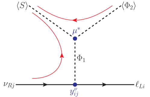
Figure 1: Feynman diagram for the neutrino mass generation. The red (black) arrows represent the flow of $U(1)_{\rm PQ}$ (lepton number) current.

Now we briefly review the mechanism for the neutrino mass generation suggested in Baek:2019wdn . The tree-level diagram shown in Fig. 1 generates the neutrino mass. The red (black) arrows represent the flow of $U(1)_{\rm PQ}$ (lepton number) current when we set $X_{\ell_{L}}=0$. The Yukawa interaction and the $\mu$-term generates the Dirac neutrino masses after the $S$ and $\Phi_{2}$ fields get VEVs:

$$m_{ij}^{\nu}=\frac{y_{ij}^{\nu}\mu v_{2}v_{S}}{2M^{2}_{\Phi_{1}}}\sim 0.1\,y_{ij}^{\nu}\left(\mu\over 1\,{\rm GeV}\right)\left(v_{2}\over 246\,{\rm GeV}\right)\left(v_{S}\over 10^{12}\,{\rm GeV}\right)\left(10^{12}\,{\rm GeV}\over M_{\Phi_{1}}\right)^{2}\,{\rm eV}.$$ (25)

The seesaw-like formula shows that the neutrino masses are ${\cal O}(0.1)$ eV for $y_{ij}^{\nu}\sim 1$, when $\mu\sim 1$ GeV, $v_{S}\sim M_{\Phi_{1}}\sim 10^{12}$ GeV. Other studies on the link between $U(1)_{\rm PQ}$ symmetry and neutrino/flavour can be found in Berezhiani:1989fp ; Gu:2006dc ; Chen:2012baa ; Dasgupta:2013cwa ; Bertolini:2014aia ; Ahn:2015pia ; Gu:2016hxh ; Ma:2017zyb ; Suematsu:2017kcu ; Ahn:2018cau ; Reig:2018yfd ; Carvajal:2018ohk ; Ahn:2019add ; delaVega:2020jcp ; CentellesChulia:2020bnf .

4 The $b\to s\mu^{+}\mu^{-}$ transition

The new colored fermions $Q_{L,R}$ induce the QCD anomaly, making $a$ an axion candidate to solve the strong CP problem. The heavy quarks (heavy leptons) can also mix with the SM quarks (leptons). The mixing can generate $Z^{\prime}-b-s$ ($Z^{\prime}-\mu-\mu$) vertex at tree-level, which can induce $b\to s\mu^{+}\mu^{-}$ transition at tree-level.

In Table 1 we introduced heavy vector-like quarks $Q_{L,R}$ and leptons $L_{L,R}$ in the same representation under the SM gauge group with $q_{L}$ and $\ell_{L}$, respectively. The heavy vector-like fermions $Q_{L}(L_{L})$ can mix with the left-handed quarks (leptons) $q_{i_{L}}(\ell_{i_{L}})$ when $\phi$ gets VEV, $v_{\phi}$. Since the $Z^{\prime}$ couples only to the left-handed quarks and leptons, we can achieve the scenario in (4).

In the CKM basis where the SM Yukawa couplings are diagonal, we can write (8) as

$${\cal L}=-(\overline{u}_{i_{L}}V^{\rm CKM}_{ij}\lambda^{q}_{j}U_{R}+\overline{d}_{i_{L}}\lambda^{q}_{i}D_{R})\phi+h.c.,$$ (26)

where we assumed the quark mixing represented by the CKM matrix $V_{\rm CKM}$ arises only in the up-quark sector. When we include the new heavy quark, the down-type quark mass matrix in the CKM basis has off-diagonal components,

$${\cal L}_{\rm mass}=-(\overline{d}_{L},\overline{s}_{L},\overline{b}_{L},\overline{D}_{L})\begin{pmatrix}m_{d}&0&0&{1\over\sqrt{2}}\lambda_{d}v_{\phi}\\ 0&m_{s}&0&{1\over\sqrt{2}}\lambda_{s}v_{\phi}\\ 0&0&m_{b}&{1\over\sqrt{2}}\lambda_{b}v_{\phi}\\ 0&0&0&M_{Q}\\ \end{pmatrix}\begin{pmatrix}d_{R}\\ s_{R}\\ b_{R}\\ D_{R}\end{pmatrix}+h.c.,$$ (27)

where $M_{Q}\equiv M_{D}=M_{U}=y_{Q}v_{S}/\sqrt{2}$, and $(\lambda_{d},\lambda_{s},\lambda_{b})\equiv(\lambda^{q}_{1},\lambda^{q}_{2},\lambda^{q}_{3})$. The corresponding up-quark mass matrix is in the same form with replacement $(m_{d},m_{s},m_{b})$ and $\lambda^{q}_{i}$ by $(m_{u},m_{c},m_{t})$ and $(V_{\rm CKM}\lambda^{q})_{i}$, respectively. The mass matrix (27) can be diagonalized by biunitary transformation:

$${\cal V}_{L}^{d\dagger}\,{\cal M}_{d}\,{\cal V}_{R}^{d}\simeq{\rm diag}(m_{d},m_{s},m_{b},M_{Q}),$$ (28)

where ${\cal M}_{d}\equiv$ (4 $\times$ 4 mass matrix) in (27). We obtain approximately

$${\cal V}_{R}^{d} \simeq{\rm diag}(1,1,1,1),$$

$${\cal V}_{L}^{d} \simeq\begin{pmatrix}1&0&0&\frac{\lambda_{d}v_{\phi}}{\sqrt{2}M_{Q}}\\ 0&1&0&\frac{\lambda_{s}v_{\phi}}{\sqrt{2}M_{Q}}\\ 0&0&1&\frac{\lambda_{b}v_{\phi}}{\sqrt{2}M_{Q}}\\ -\frac{\lambda_{d}^{*}v_{\phi}}{\sqrt{2}M_{Q}}&-\frac{\lambda_{s}^{*}v_{\phi}}{\sqrt{2}M_{Q}}&-\frac{\lambda_{b}^{*}v_{\phi}}{\sqrt{2}M_{Q}}&1\\ \end{pmatrix}.$$ (29)

The relations (28) and (29) are correct up to ${\cal O}(\lambda_{\rm max}v_{\phi}/\sqrt{2}M_{Q})^{2}$ with $\lambda_{\rm max}=\text{max}(\lambda_{d},\lambda_{s},\lambda_{b})$.

Then the effective $Z^{\prime}-s-b$ vertex for $b\to s$ transition is

$$\Lambda_{L}^{sb}\,Z^{\prime\alpha}\,\overline{s}_{L}\gamma_{\alpha}b_{L}+h.c.\equiv g_{X}\left({\cal V}_{L}^{d}\right)^{*}_{42}\left({\cal V}_{L}^{d}\right)_{43}\,Z^{\prime\alpha}\,\overline{s}_{L}\gamma_{\alpha}b_{L}+h.c.,$$ (30)

where $g_{X}$ is the $U(1)_{X}$ gauge coupling constant and

$$\Lambda_{L}^{sb}=\frac{g_{X}\lambda_{s}\lambda^{*}_{b}v_{\phi}^{2}}{2M_{Q}^{2}}.$$ (31)

This result is consistent with the one in Altmannshofer:2014cfa ; Sierra:2015fma where diagrammatic method was used. The $Z^{\prime}$ boson does not couple directly to $\mu$ either, and the effective $Z^{\prime}-\mu-\mu$ vertex is obtained by a similar procedure:

$$\Lambda_{L}^{\mu\mu}\,Z^{\prime\alpha}\,\overline{\mu}_{L}\gamma_{\alpha}\mu_{L}+h.c.,$$ (32)

where

$$\quad\Lambda_{L}^{\mu\mu}=\frac{g_{X}|\lambda_{\mu}|^{2}v_{\phi}^{2}}{2M_{L}^{2}}.$$ (33)

The prediction of Wilson coefficients $C_{9},C_{10}$ in the model can be made simply by integrating the mediating $Z^{\prime}$ gauge boson out in Fig. 2:

$$C_{9}=-C_{10}=-\frac{\pi}{\sqrt{2}G_{F}\alpha_{\rm em}}\frac{1}{V_{ts}^{*}V_{tb}}\frac{\Lambda_{L}^{sb}\Lambda_{L}^{\mu\mu}}{m_{Z^{\prime}}^{2}}.$$ (34)

By defining $x_{i}\equiv\lambda_{i}v_{\phi}/\sqrt{2}M_{Q}$, $x_{\mu}\equiv\lambda_{\mu}v_{\phi}/\sqrt{2}M_{L}$, and using the relation $m_{Z^{\prime}}=g_{X}v_{\phi}$, the above results can be rewritten as

$$C_{9}=-C_{10} =-\frac{\pi}{\sqrt{2}G_{F}\alpha_{\rm em}V_{ts}^{*}V_{tb}}\frac{x_{sb}|x_{\mu}|^{2}}{v_{\phi}^{2}}$$

$$\approx-0.43\,\left(x_{sb}\over-0.001\right)\left|x_{\mu}\over 0.5\right|^{2}\left(0.6\,{\rm TeV}\over v_{\phi}\right)^{2},$$ (35)

where $x_{sb}\equiv x_{s}x_{b}^{*}$. We can explain (4) with relatively low $v_{\phi}(=0.6\,{\rm TeV})$ when $x_{sb}=-0.001$ and $x_{\mu}=0.5$.

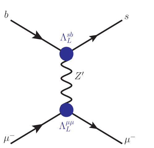
Figure 2: Feynman diagram for $b\to s\mu^{+}\mu^{-}$.

The effective vertex (30) also generates $B_{s}-\overline{B}_{s}$ mixing at tree-level, which turns out the most stringent constraint in our model Sierra:2015fma ; DiLuzio:2017fdq . In our model the effective Hamiltonian for the mixing is

$${\cal H}_{\rm eff}^{\Delta B=2}=\frac{4G_{F}}{\sqrt{2}}(V_{ts}^{*}V_{tb})^{2}[C_{sb}^{LL}(\overline{s}_{L}\gamma_{\mu}b_{L})(\overline{s}_{L}\gamma^{\mu}b_{L})+h.c.].$$ (36)

The Wilson coefficient $C_{sb}^{LL}$ is constrained by the mass difference $\Delta M_{s}$ of the $B_{s}$ system. The experimental measurement Amhis:2016xyh

$$\Delta M_{s}^{\rm exp}=(17.757\pm 0.021)\,\text{ps}^{-1}$$ (37)

is smaller than the SM prediction DiLuzio:2017fdq

$$\Delta M_{s}^{\rm SM}=(19.9\pm 1.5)\,\text{ps}^{-1}.$$ (38)

For the NP model which interferes with the SM constructively, as in our case when we take the coupling constants to be real, the constraint is very severe. The NP contributes to $C_{sb}^{LL}$ through the $Z^{\prime}$-exchanging tree-level diagram with its effective vertex in (30):

$$C_{sb}^{LL}=\frac{1}{4\sqrt{2}G_{F}(V_{ts}^{*}V_{tb})^{2}}\frac{\left(\Lambda_{L}^{sb}\right)^{2}}{m^{2}_{Z^{\prime}}}=\frac{1}{4\sqrt{2}G_{F}(V_{ts}^{*}V_{tb})^{2}}\frac{x_{sb}^{2}}{v_{\phi}^{2}}.$$ (39)

Then we get 2$\sigma$ upper bound

$$\frac{x_{sb}}{v_{\phi}}\leq 2.05\times 10^{-3}\,\text{TeV}^{-1}.$$ (40)

In Figure 3 we show the region which can explain the $b\to s\mu^{+}\mu^{-}$ puzzle in $(v_{\phi},|x_{sb}|)$ plane. The solid red line is the central value (4) to solve the $b\to s\mu^{+}\mu^{-}$ puzzle. The dashed (dotted) lines represent 1$\sigma$ (2$\sigma$) region. The gray region is diafavoured by the $B_{s}-\overline{B}_{s}$ mixing. We fixed $x_{\mu}=0.5$.

For $v_{\phi}=0.6$ TeV, $|x_{sb}|=10^{-3}$, and $|\lambda_{s}\lambda_{b}^{*}|=1$, we get $M_{Q}\approx 13$ TeV. This heavy quark mass is much smaller than the PQ-breaking scale, and therefore the Yukawa coupling should be very small $y_{Q}\sim 10^{-8}$. Since the symmetry is enhanced in the $y_{Q}\to 0$ limit, the small $y_{Q}$ is technically natural.

Since $Q_{L}(L_{L})$ has the same quantum number with the SM $q_{L}(\ell_{L})$ and $Q_{R}(L_{R})$ does not mix with the SM $u_{R},d_{R}(e_{R},\nu_{R})$, the SM $Z$ boson coupling to the SM fermions are flavour-diagonal. Therefore the $Z$-mediated FCNC interactions are not generated, which makes the constraint from the $Z$ boson interactions mild. For other constraints for the model, we refer the reader to Sierra:2015fma where possible constraints are considered in detail.

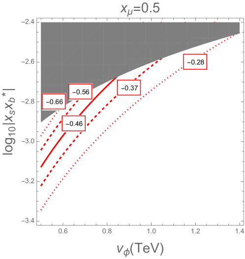
Figure 3: The solid red line is the central value (4) to solve the $b\to s\mu^{+}\mu^{-}$ puzzle. The dashed (dotted) line represents 1$\sigma$ (2$\sigma$) region. The gray region is diafavoured by the $B_{s}-\overline{B}_{s}$ mixing. We fixed $x_{\mu}=0.5$.

5 Conclusions

There are several clues which suggest new physics beyond the standard model of particle physics: dark matter, neutrino mass, strong CP problem, and possibly the flavour anomaly in $b\to s\mu^{+}\mu^{-}$ transition. We have considered a minimal model which can address the above hints simultaneously.

The neutrino mass is obtained when neutrino-specific Higgs-doublet gets a VEV, $v_{1}$ Baek:2016wml ; Baek:2018wuo ; Baek:2019wdn . The value $v_{1}$ is due to the breaking of the PQ symmetry as shown in Figure 1, is related to the high energy scale via seesaw-like relation (25), and is naturally small. Since the PQ symmetry does not allow the right-handed neutrino mass term, the neutrinos are Dirac-type.

The axion is KSVZ-type, but is distinguished from the original KSVZ model in that the axion-photon coupling is that of DFSZ-type axion model and the axion-neutrino coupling is sizable. The heavy quarks carrying PQ charges are also at 10 TeV scale without causing fine-tuning problem, and also can be tested in near future experiments.

The heavy quarks and heavy leptons also carry the charges of $U(1)_{X}$ gauge symmetry. The $U(1)_{X}$-gauge-boson-mediating tree-level diagram generates the quark-level $b\to s\mu^{+}\mu^{-}$ transition, which can explain the flavour puzzle. We considered the constraint from the existing experiments including $B_{s}-\overline{B}_{s}$ mixing.

In the model, the neutrino mass and the axion are generated by the breaking the PQ-symmetry. The PQ-charged heavy quarks which generate the QCD anomaly also induce the flavour-changing $Z^{\prime}$ couplings. The axion is also a good candidate for the cold dark matter. Therefore our model shows an interplay between neutrino mass, flavour physics, axion, and dark matter.

- (1) S. Baek, Dirac neutrino from the breaking of Peccei-Quinn symmetry, Phys. Lett. B805 (2020) 135415, [1911.04210].
- (2) S. Baek and T. Nomura, Dark matter physics in neutrino specific two Higgs doublet model, JHEP 03 (2017) 059, [1611.09145].
- (3) S. Baek, A. Das and T. Nomura, Scalar dark matter search from the extended THDM, JHEP 05 (2018) 205, [1802.08615].
- (4) G. Buchalla, A. J. Buras and M. E. Lautenbacher, Weak decays beyond leading logarithms, Rev. Mod. Phys. 68 (1996) 1125–1144, [hep-ph/9512380].
- (5) S. Baek and P. Ko, Probing SUSY induced CP violations at B factories, Phys. Rev. Lett. 83 (1999) 488–491, [hep-ph/9812229].
- (6) S. Baek, T. Goto, Y. Okada and K.-i. Okumura, Neutrino oscillation, SUSY GUT and B decay, Phys. Rev. D 63 (2001) 051701, [hep-ph/0002141].
- (7) S. Baek, P. Ko and W. Y. Song, Implications on SUSY breaking mediation mechanisms from observing B(s) —> mu+ mu- and the muon (g-2), Phys. Rev. Lett. 89 (2002) 271801, [hep-ph/0205259].
- (8) LHCb collaboration, R. Aaij et al., Search for lepton-universality violation in decays, Phys. Rev. Lett. 122 (2019) 191801, [1903.09252].
- (9) LHCb collaboration, R. Aaij et al., Test of lepton universality with decays, JHEP 08 (2017) 055, [1705.05802].
- (10) Belle collaboration, A. Abdesselam et al., Test of lepton flavor universality in decays at Belle, 1904.02440.
- (11) M. Algueró, B. Capdevila, A. Crivellin, S. Descotes-Genon, P. Masjuan, J. Matias et al., Emerging patterns of New Physics with and without Lepton Flavour Universal contributions, Eur. Phys. J. C 79 (2019) 714, [1903.09578].
- (12) A. K. Alok, A. Dighe, S. Gangal and D. Kumar, Continuing search for new physics in decays: two operators at a time, JHEP 06 (2019) 089, [1903.09617].
- (13) M. Ciuchini, A. M. Coutinho, M. Fedele, E. Franco, A. Paul, L. Silvestrini et al., New Physics in confronts new data on Lepton Universality, Eur. Phys. J. C 79 (2019) 719, [1903.09632].
- (14) A. Datta, J. Kumar and D. London, The anomalies and new physics in , Phys. Lett. B 797 (2019) 134858, [1903.10086].
- (15) J. Aebischer, W. Altmannshofer, D. Guadagnoli, M. Reboud, P. Stangl and D. M. Straub, B-decay discrepancies after Moriond 2019, Eur. Phys. J. C 80 (2020) 252, [1903.10434].
- (16) K. Kowalska, D. Kumar and E. M. Sessolo, Implications for new physics in transitions after recent measurements by Belle and LHCb, Eur. Phys. J. C 79 (2019) 840, [1903.10932].
- (17) A. Arbey, T. Hurth, F. Mahmoudi, D. M. Santos and S. Neshatpour, Update on the bs anomalies, Phys. Rev. D 100 (2019) 015045, [1904.08399].
- (18) D. Aristizabal Sierra, F. Staub and A. Vicente, Shedding light on the anomalies with a dark sector, Phys. Rev. D 92 (2015) 015001, [1503.06077].
- (19) P. Arnan, L. Hofer, F. Mescia and A. Crivellin, Loop effects of heavy new scalars and fermions in , JHEP 04 (2017) 043, [1608.07832].
- (20) J. M. Cline, J. M. Cornell, D. London and R. Watanabe, Hidden sector explanation of -decay and cosmic ray anomalies, Phys. Rev. D 95 (2017) 095015, [1702.00395].
- (21) J. Kawamura, S. Okawa and Y. Omura, Interplay between the b anomalies and dark matter physics, Phys. Rev. D 96 (2017) 075041, [1706.04344].
- (22) S. Baek, Dark matter contribution to anomaly in local model, Phys. Lett. B 781 (2018) 376–382, [1707.04573].
- (23) J. M. Cline, decay anomalies and dark matter from vectorlike confinement, Phys. Rev. D 97 (2018) 015013, [1710.02140].
- (24) C.-W. Chiang and H. Okada, A simple model for explaining muon-related anomalies and dark matter, Int. J. Mod. Phys. A 34 (2019) 1950106, [1711.07365].
- (25) J. M. Cline and J. M. Cornell, from dark matter exchange, Phys. Lett. B 782 (2018) 232–237, [1711.10770].
- (26) A. Vicente, Anomalies in transitions and dark matter, Adv. High Energy Phys. 2018 (2018) 3905848, [1803.04703].
- (27) A. Falkowski, S. F. King, E. Perdomo and M. Pierre, Flavourful portal for vector-like neutrino Dark Matter and , JHEP 08 (2018) 061, [1803.04430].
- (28) S. Baek and C. Yu, Dark matter for anomaly in a gauged model, JHEP 11 (2018) 054, [1806.05967].
- (29) L. Darmé, K. Kowalska, L. Roszkowski and E. M. Sessolo, Flavor anomalies and dark matter in SUSY with an extra U(1), JHEP 10 (2018) 052, [1806.06036].
- (30) B. Barman, D. Borah, L. Mukherjee and S. Nandi, Correlating the anomalous results in decays with inert Higgs doublet dark matter and muon , Phys. Rev. D 100 (2019) 115010, [1808.06639].
- (31) S. Singirala, S. Sahoo and R. Mohanta, Exploring dark matter, neutrino mass and anomalies in model, Phys. Rev. D 99 (2019) 035042, [1809.03213].
- (32) A. Vicente, Flavor and Dark Matter connection, Springer Proc. Phys. 234 (2019) 393–400, [1812.03028].
- (33) S. Baek, Scalar dark matter behind anomaly, JHEP 05 (2019) 104, [1901.04761].
- (34) D. Cerdeño, A. Cheek, P. Martín-Ramiro and J. Moreno, B anomalies and dark matter: a complex connection, Eur. Phys. J. C 79 (2019) 517, [1902.01789].
- (35) P. Ko, T. Nomura and C. Yu, anomalies and related phenomenology in flavor gauge models, JHEP 04 (2019) 102, [1902.06107].
- (36) A. Biswas and A. Shaw, Reconciling dark matter, anomalies and in an scenario, JHEP 05 (2019) 165, [1903.08745].
- (37) P. Arnan, A. Crivellin, M. Fedele and F. Mescia, Generic loop effects of new scalars and fermions in and a vector-like generation, JHEP 06 (2019) 118, [1904.05890].
- (38) S. Trifinopoulos, B -physics anomalies: The bridge between R -parity violating supersymmetry and flavored dark matter, Phys. Rev. D 100 (2019) 115022, [1904.12940].
- (39) Z.-L. Han, R. Ding, S.-J. Lin and B. Zhu, Gauged scotogenic model in light of anomaly and AMS-02 positron excess, Eur. Phys. J. C 79 (2019) 1007, [1908.07192].
- (40) L. Darmé, M. Fedele, K. Kowalska and E. M. Sessolo, Flavour anomalies from a split dark sector, 2002.11150.
- (41) J. E. Kim, Weak Interaction Singlet and Strong CP Invariance, Phys. Rev. Lett. 43 (1979) 103.
- (42) M. A. Shifman, A. I. Vainshtein and V. I. Zakharov, Can Confinement Ensure Natural CP Invariance of Strong Interactions?, Nucl. Phys. B166 (1980) 493–506.
- (43) R. Foot, A. Kobakhidze, K. L. McDonald and R. R. Volkas, Poincaré protection for a natural electroweak scale, Phys. Rev. D 89 (2014) 115018, [1310.0223].
- (44) R. Peccei, The Strong CP problem and axions, Lect. Notes Phys. 741 (2008) 3–17, [hep-ph/0607268].
- (45) M. Srednicki, Axion Couplings to Matter. 1. CP Conserving Parts, Nucl. Phys. B260 (1985) 689–700.
- (46) M. Dine, W. Fischler and M. Srednicki, A Simple Solution to the Strong CP Problem with a Harmless Axion, Phys. Lett. 104B (1981) 199–202.
- (47) A. R. Zhitnitsky, On Possible Suppression of the Axion Hadron Interactions. (In Russian), Sov. J. Nucl. Phys. 31 (1980) 260.
- (48) G.-Y. Huang and N. Nath, Neutrinophilic Axion-Like Dark Matter, Eur. Phys. J. C 78 (2018) 922, [1809.01111].
- (49) Z. G. Berezhiani and M. Yu. Khlopov, Cosmology of Spontaneously Broken Gauge Family Symmetry, Z. Phys. C49 (1991) 73–78.
- (50) P.-H. Gu and H.-J. He, Neutrino Mass and Baryon Asymmetry from Dirac Seesaw, JCAP 0612 (2006) 010, [hep-ph/0610275].
- (51) C.-S. Chen and L.-H. Tsai, Peccei-Quinn symmetry as the origin of Dirac Neutrino Masses, Phys. Rev. D88 (2013) 055015, [1210.6264].
- (52) B. Dasgupta, E. Ma and K. Tsumura, Weakly interacting massive particle dark matter and radiative neutrino mass from Peccei-Quinn symmetry, Phys. Rev. D89 (2014) 041702, [1308.4138].
- (53) S. Bertolini, L. Di Luzio, H. Kolešová and M. Malinský, Massive neutrinos and invisible axion minimally connected, Phys. Rev. D91 (2015) 055014, [1412.7105].
- (54) Y. H. Ahn and E. J. Chun, Minimal Models for Axion and Neutrino, Phys. Lett. B752 (2016) 333–337, [1510.01015].
- (55) P.-H. Gu, Peccei-Quinn symmetry for Dirac seesaw and leptogenesis, JCAP 1607 (2016) 004, [1603.05070].
- (56) E. Ma, D. Restrepo and Ó. Zapata, Anomalous leptonic U(1) symmetry: Syndetic origin of the QCD axion, weak-scale dark matter, and radiative neutrino mass, Mod. Phys. Lett. A33 (2018) 1850024, [1706.08240].
- (57) D. Suematsu, Dark matter stability and one-loop neutrino mass generation based on Peccei–Quinn symmetry, Eur. Phys. J. C78 (2018) 33, [1709.02886].
- (58) Y. H. Ahn, Compact model for Quarks and Leptons via flavored-Axions, Phys. Rev. D98 (2018) 035047, [1804.06988].
- (59) M. Reig and R. Srivastava, Spontaneous proton decay and the origin of Peccei–Quinn symmetry, Phys. Lett. B790 (2019) 134–139, [1809.02093].
- (60) C. D. R. Carvajal and Ó. Zapata, One-loop Dirac neutrino mass and mixed axion-WIMP dark matter, Phys. Rev. D99 (2019) 075009, [1812.06364].
- (61) Y. Ahn and X. Bi, Predictions of QCD axion and Neutrino induced by Hidden flavor structure, 1912.09038.
- (62) L. M. de la Vega, N. Nath and E. Peinado, Dirac neutrinos from Peccei-Quinn symmetry: two examples, 2001.01846.
- (63) S. Centelles Chuliá, C. Döring, W. Rodejohann and U. J. Saldaña-Salazar, Natural axion model from flavour, 2005.13541.
- (64) W. Altmannshofer, S. Gori, M. Pospelov and I. Yavin, Quark flavor transitions in models, Phys. Rev. D 89 (2014) 095033, [1403.1269].
- (65) L. Di Luzio, M. Kirk and A. Lenz, Updated -mixing constraints on new physics models for anomalies, Phys. Rev. D 97 (2018) 095035, [1712.06572].
- (66) HFLAV collaboration, Y. Amhis et al., Averages of -hadron, -hadron, and -lepton properties as of summer 2016, Eur. Phys. J. C 77 (2017) 895, [1612.07233].