Spectral convergence of diffusion maps: improved error bounds and an alternative normalisation

Abstract

Diffusion maps is a manifold learning algorithm widely used for dimensionality reduction. Using a sample from a distribution, it approximates the eigenvalues and eigenfunctions of associated Laplace-Beltrami operators. Theoretical bounds on the approximation error are however generally much weaker than the rates that are seen in practice. This paper uses new approaches to improve the error bounds in the model case where the distribution is supported on a hypertorus. For the data sampling (variance) component of the error we make spatially localised compact embedding estimates on certain Hardy spaces; we study the deterministic (bias) component as a perturbation of the Laplace-Beltrami operator’s associated PDE, and apply relevant spectral stability results. Using these approaches, we match long-standing pointwise error bounds for both the spectral data and the norm convergence of the operator discretisation.

We also introduce an alternative normalisation for diffusion maps based on Sinkhorn weights. This normalisation approximates a Langevin diffusion on the sample and yields a symmetric operator approximation. We prove that it has better convergence compared with the standard normalisation on flat domains, and present a highly efficient algorithm to compute the Sinkhorn weights.

35P15, 60J60, 62M05, 65D99

1 Introduction

Many problems in data science revolve around the extraction of information about the geometry of some probability distribution given only a sample that may possibly be embedded in an ambient space of much higher dimension: examples of these problems include clustering and dimension reduction. The intrinsic geometry of such a distribution may be encoded by various weighted Laplace-Beltrami operators, from whose spectral data various desiderata can be extracted: for example, the operator’s eigenfunctions may be used to define intrinsic coordinates for the support of the distribution (Coifman et al. 2005, Coifman & Lafon 2006), or may be used in spectral clustering algorithms (Nadler et al. 2006).

Diffusion maps is a widely-used algorithm to recover the relevant eigendata (Coifman et al. 2005, Coifman & Lafon 2006): the idea is to construct a particle discretisation of the evolution of a weighted Laplace-Beltrami operator $\mathcal{L}$ over some short timestep $\varepsilon$. To this end, a kernel matrix $K$ is first constructed:

(1) $$K=\left(\tfrac{1}{M}k_{\varepsilon}(d(x^{i},x^{j}))\right)_{i,j=1,\ldots,M},$$

where the $x^{i}\sim\rho\,{\rm d}x$ are the sample points, $k_{\varepsilon}$ is a symmetric probability kernel with covariance matrix $\varepsilon I$. The kernel matrix is then normalised to be Markov (i.e. row-stochastic)

(2) $$P=\operatorname{diag}(Ku)^{-1}K\operatorname{diag}(u),$$

for some appropriately chosen weight vector $u\in\mathbb{R}^{M}$.

As the sample size $M$ is taken to infinity and the diffusion timestep $\varepsilon$ is taken to zero with an appropriate dependence on $M$ (Lindenbaum et al. 2017), the spectral data of $P$ should approximate that of the Laplace-Beltrami operator semigroup $e^{\varepsilon\mathcal{L}}$, enabling reconstruction of the spectral data of the operator $\mathcal{L}$ itself. (Indeed, this problem is often formulated as the graph Laplacian $L=\varepsilon^{-1}(P-I)$ approximating $\mathcal{L}$.) The Markov nature of the normalised matrix $P$ means that the intrinsic coordinates provided by its leading eigenvectors faithfully reconstruct the intrinsic geometry of the distribution’s support (Coifman & Lafon 2006).

Standard choices of weights for these operators are of the form $\check{u}_{\alpha}\equiv(K1)^{-\alpha}$, for some $\alpha\in[0,1]$. In this case, the weighted Laplace-Beltrami operators to which the convergence occurs are

(3) $$\check{\mathcal{L}}_{\alpha}\phi:=\tfrac{1}{2}\Delta\phi+(1-\alpha)\nabla\log\rho\cdot\nabla\phi=\tfrac{1}{2}\rho^{-(2-2\alpha)}\,\nabla\cdot(\rho^{2-2\alpha}\nabla\phi),$$

where $\rho$ is the density of the distribution with respect to Lebesgue measure. The case $\alpha=0$ (i.e. $\check{u}\equiv 1$) is the standard graph Laplacian normalisation; on the other hand, we recover for $\alpha=1$ the unweighted Laplace-Beltrami operator, and for $\alpha=\tfrac{1}{2}$ the generator of the Langevin diffusion with invariant measure $\rho$ (Coifman & Lafon 2006).

The last twenty years have seen a range of rigorous work establishing and bounding the convergence of diffusion maps and related methods. Because both a space and time discretisation occur, the error decomposes into two parts: a “variance” error of finite samples size $M$ with the timestep $\varepsilon$ held fixed, and a “bias” error from the positive timestep $\varepsilon$, which is independent of $M$. (Often instead of the timestep, the kernel bandwidth $\varepsilon^{1/2}$ is used, sometimes notated by $h$ or $\epsilon$.) For pointwise estimates on the kernel matrix $P$, the errors associated with the two limits have been shown to be bounded respectively by $\mathcal{O}(M^{-1/2}\varepsilon^{-d/4})$ (Hein et al. 2005) and, on flat manifolds, $\mathcal{O}(\varepsilon^{2})$ (Singer 2006). There are clear intuitions to these error rates: the first is a central limit theorem error between $K$ and its infinite data limit, taking into account that of the $M$ sample points, we expect $M_{\mathrm{eff}}=\mathcal{O}(M\varepsilon^{d/2})$ to be in the effective support of the kernel; the second is a standard first-order discretisation error for a diffusion operator over timestep $\varepsilon$. It is natural to expect that the pointwise error of the discretisation should transfer to the spectral data: with the short timestep magnifying the errors by a factor of $\mathcal{O}(\varepsilon^{-1})$, this would yield an $\mathcal{O}(M^{-2/(8+d)})$ error for the optimal scaling of $\varepsilon$ with $M$.

However, theoretical estimates for spectral data in the literature have been much weaker than this. The standard bound on the bias error in the spectral data, in both $L^{2}$ and $L^{\infty}$ norms, has been the naive estimate of $\mathcal{O}(\varepsilon^{1/2})$, corresponding to the $L^{p}\to L^{p}$ operator error (Hein et al. 2005, Shi 2015, Trillos et al. 2019, Lu 2020, Dunson et al. 2019).

While the decay of the variance error as $M\to\infty$ with $\varepsilon$ fixed has been long known using compact embedding of Glivenko-Cantelli function classes (von Luxburg et al. 2004, 2008, Belkin & Niyogi 2007, Dunson et al. 2019), this approach has yielded only weak quantitative bounds on the variance error, the best to date being $\mathcal{O}(M^{-1/2}\varepsilon^{-d-3})$ in $L^{\infty}$ (Shi 2015). Due to the dependence of the weights $\check{u}_{\alpha}$ on the sample for $\alpha\neq 0$, this approach has also largely been specialised to the graph Laplacian normalisation $\alpha=0$. More recently optimal transport techniques have been applied to bound the variance error. These necessarily sacrifice the central limit theorem convergence in $M$ for the much slower optimal transport rate of $\mathcal{O}((\tfrac{\log M}{M})^{1/d})$, but yield an overall error of $\mathcal{O}((\tfrac{\log M}{M})^{1/2d})$ in the eigenvalues for dimensions $d\geq 2$ (Trillos et al. 2019, Lu 2020).

In Calder & Trillos (2019) these results were bootstrapped with (weaker) pointwise estimates to obtain a central limit theorem convergence in $M$ with overall $L^{2}$-convergence rate of $\mathcal{O}((\tfrac{\log M}{M})^{1/(d+4)})$ on general manifolds (although this was based on an assumption of $O(\varepsilon^{1/2})$ bias error on curved manifolds). However, only unweighted graph Laplacians were studied: more complex kernel estimation problems will require increasingly more complex concentration of measure estimates to obtain pointwise convergence. Furthermore, the spectral convergence was obtained from pointwise convergence via Rayleigh quotients, which are specific to self-adjoint operators.

The first goal of our paper is to prove that for diffusion maps normalisations, the pointwise error bounds hold for the spectral data. This work is independent of Calder & Trillos (2019) and takes a different, more dynamical approach that may in fact be applied very generally to Gaussian kernel-based discretisation problems. This is because we fully carry through the pointwise convergence rates of diffusion maps discretisations to norm convergence of the discretised operators. For simplicity, we will assume the support of the measure is a flat torus $\mathbb{D}=(\mathbb{R}/L\mathbb{Z})^{d}$ and the sample points $x^{i}$ are independent and identically distributed; we will use the standard Gaussian choice of kernel. Our only assumptions on the sample density $\rho$ are that it is bounded away from zero and $C^{3/2+\beta}$ Hölder for some $\beta>0$ (i.e. a $C^{\beta^{\prime}}$ first derivative for some $\beta>1/2$). We will show that convergence of eigenfunctions holds in the space $C^{0}$ of continuous functions (i.e. in $L^{\infty}$ norm).

To achieve this goal we will apply new approaches to both the bias and variance components of the error. To bound the bias error, we will reformulate the problem as one of compact PDE evolution operators for which the perturbations are bounded from a strong norm to a weak norm, and apply the relevant spectral approximation theory (Keller & Liverani 1999). For the standard weights, this is a more or less straightforward result in approximation of diffusion semigroups, except that we apply the theory of negative Sobolev spaces obtain convergence for $\rho$ of relatively low regularity. For the Sinkhorn weights discussed below, we will combine this with an averaging argument to prove the faster convergence.

On the other hand, our bounds on the variance error conservatively extend the pointwise error bound for kernels to operator errors in certain Hardy spaces via localised compact embedding estimates. These embedding estimates are obtained by considering Glivenko-Cantelli function classes on small subsets of the domain and harnessing the localisation of the kernel. The enabling factors in our techniques are thus the kernel function’s smoothness (in Proposition 8.7) and its fast decay away from zero (in Proposition 8.10); these results do not rely on differentiability of the sampling measure or of the underlying manifold, nor in fact do they rely on the Markov nature of the operator.

Combining these, we will obtain a spectral error of $\mathcal{O}(M^{-1/2}\varepsilon^{-1-d/4}(\log M\varepsilon^{-1})^{d-1/2}+\varepsilon)$. With optimal scaling $\varepsilon\sim M^{-2/(8+d)+o_{M}(1)}$, this gives a total error of $\mathcal{O}(M^{-2/(8+d)+o_{M}(1)})$. For larger dimensions $d\geq 3$, this is a major improvement over previous results for weighted Laplacians: for example, compared with Trillos et al. (2019) the accuracy is squared for $d=8$. It is also a significant improvement on the unweighted Laplacian results of Calder & Trillos (2019). Our convergence rate for the variance error of spectral data estimates still remains somewhat weaker than variance errors observed empirically. This is partly because we obtain convergence results for normalised operators directly from the convergence of the unnormalised kernel: we expect that making use of the Markov nature of the semigroup will give an $\mathcal{O}(\varepsilon^{1/2})$ improvement in variance error (Singer 2006), bringing it into line with previous results in the regime of pointwise convergence (Calder & Trillos 2019), to which our $L^{\infty}$ results must necessarily be limited. On the other hand, the $\mathcal{O}(\varepsilon)$ bias error bound appears optimal. These rates can be expected to carry across to general curved manifolds (for the bias error this was observed in Vaughn et al. (2019)).

Our theoretical approach facilitates the second goal of the paper: to study a superior normalisation using Sinkhorn weights for the Langevin dynamics whose generator is

(4) $$\mathcal{L}\phi:=\check{\mathcal{L}}_{0.5}\phi=\tfrac{1}{2}\Delta\phi+\tfrac{1}{2}\nabla\log\rho\cdot\nabla\phi.$$

So-called Sinkhorn weights $u,\,1/(Ku)$ for a general matrix $K$ are defined to be those making the row-stochastic matrix $P=\operatorname{diag}(Ku)^{-1}K\operatorname{diag}(u)$ also column-stochastic. This kind of matrix weighting problem has been studied since Sinkhorn (1964); it has been studied in the context of image processing (Kheradmand & Milanfar 2014) and in spectral clustering (Brand & Huang 2003, Wang et al. 2012, 2016, 2020); it has seen interest in the context of computing entropically regularised optimal transport plans (Cuturi 2013, Altschuler et al. 2017, Feydy et al. 2019), and has been recently been considered as a diffusion maps normalisation (Marshall & Coifman 2019). The Sinkhorn (also known as bi-stochastic or doubly stochastic) normalisation has been found to have superior properties to many standard Markovian kernels in many applications (Wang et al. 2020, Landa et al. 2020). In using Sinkhorn weights as a normalisation for diffusion maps, we will study the restricted case where the kernel matrix $K$ is symmetric (and so one is computing a coupling of the sample’s empirical measure $\rho^{M}$ with itself). In this restricted case, such weights solve the (quadratic) problem

(5) $$\operatorname{diag}(u)=\operatorname{diag}(Ku)^{-1}.$$

We will prove that, at least in the cases we consider, the Sinkhorn weights have an improved rate of convergence, with the bias error in eigendata improving to $\mathcal{O}(\varepsilon^{2})$ from $\mathcal{O}(\varepsilon)$ for standard weights, and the variance error remaining the same. This means that, compared with the standard weights, a larger timestep $\varepsilon\sim M^{-2/(12+d)+o(1)}$ may be chosen with a further improved overall convergence rate of $\mathcal{O}(M^{-4/(12+d)+o(1)})$, although in practice $\varepsilon$ has to be rather small, and thus $M$ very large, for this convergence rate to take hold. For this convergence to hold it is only necessary that the density $\rho$ be $C^{2+\beta}$ Hölder for $\beta>0$.

While Sinkhorn weights must be computed iteratively, we also present an accelerated algorithm to calculate the weights that, by harnessing the symmetric nature of the problem, converges in $\mathcal{O}(1)$ matrix-vector multiplications. This algorithm was first noted by Marshall & Coifman (2019): here we establish a convergence rate, with rigorous bounds. As a result, use of Sinkhorn weights has minimal numerical overhead.

This paper is structured as follows. In Section 2 we define the mathematical objects used in the paper; in Section 3 we state the main theorems with a brief numerical illustration; in Section 4 we describe our accelerated Sinkhorn algorithm. We then turn to studying the convergence of relevant operators as the timestep $\varepsilon\to 0$, focussing on the more interesting case of the Sinkhorn normalisation. After stating some relevant functional-analytic results in Section 5 and describing the convergence of Sinkhorn weights as $\varepsilon\to 0$ in Section 6, we prove the necessary operator convergence result for the bias error in Section 7. We then consider the variance error, i.e.  that of finite $M$: in Section 8 we bound the operator convergence of the kernel matrix $K$ to a continuum limit in appropriate norms, and in Section 9 we do the same for the normalised matrix $P$; in Section 10 we combine the two operator convergence results to prove the convergence of spectral data for the Sinkhorn weight case. Finally, we outline the corresponding results for standard weights in Section 11.

2 Notation

We now present some notation that will be used in the main theorems and throughout the paper. Notation used throughout this paper is tabulated in Tables 1-2.

$d$	The dimension of the domain
$L$	The side length of the domain
$\mathbb{D}$	The domain of the problem, a hypertorus (see Section 2.1)
$\rho$	The sampling density
$\varepsilon$	The timestep parameter; $\varepsilon^{1/2}$ the kernel bandwidth
$M$	The number of data points in the sample
$M_{\mathrm{eff}}$	The effective number of points in the bandwidth of the kernel
$x^{i}$	A data point sampled from $\rho$
$\rho^{M}$	The empirical measure of the sample $\{x_{i}\}_{i=1,\ldots,M}$
$\alpha$	The parameter for diffusion maps weights (see Section 1)
$\beta$	A Hölder parameter in $(0,1)$
$\delta$	The norm of an operator quantifying the variance error (see $(\ref{eq:DeltaDef})$)
$r,s$	Sobolev space differentiability parameters
$\lambda_{*}$	A ceiling on the magnitude of eigenvalues considered for convergence
$\zeta$	The width in the complex direction of $\mathbb{D}_{\zeta}$
$Z_{0}$	The constant of the scaling between $\zeta$ and $\varepsilon^{1/2}$
$\mathbb{D}_{\zeta}$	A complex fattening of the real domain $\mathbb{D}$ by $\zeta$ (see Section 2.2)
$g_{\varepsilon}$	The Gaussian kernel on $\mathbb{R}^{d}$
$g_{\varepsilon,L}$	The periodised Gaussian kernel on $\mathbb{D}$ (see Section 2.1)
$\gamma_{\varepsilon,L},\gamma^{\prime}_{\varepsilon,L}$	Small constants relating to the periodisation of the Gaussian kernel (see 8.2)
$\sigma$	The square root of the density, $\rho^{1/2}$ (see Section 6)
$u^{(n)}$	The $n$th iterate of matrix-vector Sinkhorn iteration (see Section 4)
$U^{(n)}$	The $n$th iterate of Sinkhorn iteration in function space (see Sections 4 and 6)
$w^{t}_{\varepsilon}$	The odd limit cycle of $(\ref{eq:SinkhornPDE})$
$\hat{w}^{t}_{\varepsilon}$	The periodic drift term in the PDE $(\ref{eq:SDMPDE})$
$\mathcal{L}$	The generator of the Langevin diffusion PDE $(\ref{eq:Generator})$
$\check{\mathcal{L}}_{\alpha}$	The generator of the diffusion PDE $(\ref{eq:GeneratorStandard})$
$S_{\varepsilon}$	The solution operator of the PDE $(\ref{eq:SDMPDE})$
$\check{S}_{\alpha,\varepsilon}$	The solution operator of the PDE $(\ref{eq:SDMPDEStandard})$
$J$	The Bessel operator $I-\Delta$ (see Section 2.2)
$K^{\cdot}_{\cdot}$	Various constants regarding Sobolev space inclusions (see Proposition 5.1)
$Z$	The vector space of functions that integrate to zero
$H^{\infty}(\mathbb{D}_{\zeta})$	The Hardy space of bounded analytic functions on $\mathbb{D}_{\zeta}$ (see Section 2.2)
$R_{\lambda}(\cdot)$	The resolvent at $\lambda$ (see $(\ref{eq:ResolventDef})$)
$\|\cdot\|_{0}$	The $C^{0}$ norm
$\|\cdot\|_{\zeta}$	The $H^{\infty}(\mathbb{D}_{\zeta})$ norm
$\|\cdot\|_{s,p}$	The $W^{s,p}$ norm
$d_{C^{0}}(\cdot,\cdot)$	The $C^{0}$ distance between eigenspaces (see $(\ref{eq:dCO})$)

Table 1: List of symbols (see also Table 2)

Gene-rator	Semi-group	Finite $\varepsilon$	Finite $M,\varepsilon$	Matx/ vector
$\Delta/2$	$\mathcal{C}_{\varepsilon}$				The Gaussian diffusion operator (see $(\ref{eq:Convolution})$)
		$\mathcal{K}_{\varepsilon}$	$\mathcal{K}^{M}_{\varepsilon}$	$K$	The unweighted kernel operator (see (9, 12, 1))
		$\rho_{\varepsilon}$	$\rho^{M}_{\varepsilon}$		The measure, slightly diffused (see $(\ref{eq:RhoEpsDef})$)
Sinkhorn weights
		$U_{\varepsilon}$	$U^{M}_{\varepsilon}$	$u$	The weight function (see Section 2.1, $(\ref{eq:SinkhornWeightsDiscrete})$)
$\mathcal{L}$	$e^{\varepsilon\cal L}$	$\mathcal{P}_{\varepsilon}$	$\mathcal{P}^{M}_{\varepsilon}$	$P$	The (Sinkhorn) weighted operator (see (11, 14, 2))
		$Y_{\varepsilon}$	$Y^{M}_{\varepsilon}$		The half-step (Sinkhorn) weight (see $(\ref{eq:Y})$)
		$\mathcal{G}_{\varepsilon}$	$\mathcal{G}^{M}_{\varepsilon}$		The left half-step operator (see $(\ref{eq:J})$)
		$\mathcal{H}_{\varepsilon}$	$\mathcal{H}^{M}_{\varepsilon}$		The right half-step operator (see $(\ref{eq:K})$)
		$\mathcal{Q}_{\varepsilon,n}$	$\mathcal{Q}^{M}_{\varepsilon,n}$		The semiconjugacy of $\mathcal{P}^{n}$ by half-step (see $(\ref{eq:M})$)
$-\lambda_{k}$	$e^{-\varepsilon\lambda_{k}}$	$e^{-\varepsilon\lambda_{k,\varepsilon}}$	$e^{-\varepsilon\lambda^{M}_{k,\varepsilon}}$		The $k$th eigenvalue of $\mathcal{L}$/$\mathcal{P}$ (see Section 2.3)
$-\lambda_{k}$		$-\tilde{\lambda}_{k,\varepsilon}$	$-\tilde{\lambda}^{M}_{k,\varepsilon}$		The $k$th graph Laplacian eigenvalue (see Section 27)
$E_{k}$	$E_{k}$	$\bar{E}_{k,\varepsilon}$	$\bar{E}^{M}_{k,\varepsilon}$		The $k$th eigenspace of $\mathcal{L}$/$\mathcal{P}$ (see Section 2.3)
$\Pi_{k}$	$\Pi_{k}$	$\Pi_{k,\varepsilon}$	$\Pi^{M}_{k,\varepsilon}$		The $k$th spectral projection operator (see $(\ref{eq:SemigroupProjectionDefinition}-\ref{eq:ProjectionDefinition})$)
Standard weights
		$\check{U}_{\varepsilon,\alpha}$	$\check{U}^{M}_{\varepsilon,\alpha}$	$\check{u}_{\alpha}$	The right-hand (standard) weight function (see $(\ref{eq:StandardDiscretisationU})$)
		$\check{V}_{\varepsilon,\alpha}$	$\check{V}^{M}_{\varepsilon,\alpha}$		The left-hand (standard) weight function (see $(\ref{eq:StandardDiscretisationV})$)
$\check{\mathcal{L}}_{\alpha}$	$e^{\varepsilon\check{\mathcal{L}}_{\alpha}}$	$\check{\mathcal{P}}_{\varepsilon,\alpha}$	$\check{\mathcal{P}}^{M}_{\varepsilon,\alpha}$		The (standard) weighted operator (see $(\ref{eq:StandardDiscretisationP})$)
		$\check{Y}_{\varepsilon}$	$\check{Y}^{M}_{\varepsilon}$		The half-step weight function (see $(\ref{eq:YStandard})$)
		$\check{\mathcal{G}}_{\varepsilon,\alpha}$	$\check{\mathcal{G}}^{M}_{\varepsilon,\alpha}$		The left half-step operator (see $(\ref{eq:JStandard})$)
		$\check{\mathcal{H}}_{\varepsilon,\alpha}$	$\check{\mathcal{H}}^{M}_{\varepsilon,\alpha}$		The right half-step operator (see $(\ref{eq:KStandard})$)
		$\check{\mathcal{Q}}_{\varepsilon,n}$	$\check{\mathcal{Q}}^{M}_{\varepsilon,n}$		The semiconjugacy of $\check{\mathcal{P}}^{n}$ by half-step (see $(\ref{eq:MStandard})$)
$-\check{\lambda}_{k,\alpha}$	$e^{-\varepsilon\check{\lambda}_{k,\alpha}}$	$e^{-\varepsilon\check{\lambda}_{k,\varepsilon,\alpha}}$	$e^{-\varepsilon\check{\lambda}^{M}_{k,\varepsilon,\alpha}}$		The $k$th eigenvalue of $\check{\mathcal{L}}$/$\check{\mathcal{P}}$ (see Section 2.3)
$-\check{\lambda}_{k,\alpha}$		$-\check{\tilde{\lambda}}_{k,\varepsilon,\alpha}$	$-\check{\tilde{\lambda}}^{M}_{k,\varepsilon,\alpha}$		The $k$th graph Laplacian eigenvalue (see $(\ref{eq:GraphLaplacianEigenvaluesStandard})$)
$\check{E}_{k,\alpha}$	$\check{E}_{k,\alpha}$	$\check{\bar{E}}_{k,\varepsilon,\alpha}$	$\check{\bar{E}}^{M}_{k,\varepsilon,\alpha}$		The $k$th eigenspace of $\check{\mathcal{L}}$/$\check{\mathcal{P}}$ (see Section 2.3)

Table 2: List of symbols dependent on different limits. Where a reference is not given for standard weights quantities, they are defined by analogy with the Sinkhorn equivalent.

2.1 Operators

Recall that our domain is $\mathbb{D}=(\mathbb{R}/L\mathbb{Z})^{d}$. We will use as our kernel function the periodic Gaussian kernel $k_{\varepsilon}(x,y)=g_{\varepsilon,L}(y-x)$:

(6) $$g_{\varepsilon,L}(x) =\sum_{\mathbf{j}\in\mathbb{Z}^{d}}g_{\varepsilon}(x+L\mathbf{j}),$$

where the standard Gaussian kernel is

(7) $$g_{\varepsilon}(x) =(2\pi\varepsilon)^{-d/2}e^{-\|x\|^{2}/2\varepsilon}.$$

Note that if, as is typical, the bandwidth $\sqrt{\varepsilon}\ll L$, all but one summand in $(\ref{eq:GaussianKernelL})$ will be superexponentially small.

We define convolution by the periodic Gaussian kernel $(\ref{eq:GaussianKernelL})$ as an operator

(8) $$(\mathcal{C}_{\varepsilon}\phi)(x)=\int_{\mathbb{D}}g_{\varepsilon,L}(y-x)\phi(y)\,{\rm d}x,$$

which has the semigroup property $\mathcal{C}_{s}\mathcal{C}_{t}=\mathcal{C}_{s+t}$.

In this paper we will interpolate the vectors and matrices introduced in the introduction by functions defined on the continuous domain $\mathbb{D}$. Our interpolation arises very naturally: the kernel matrix $K$ defined in $(\ref{eq:KernelMatrix})$ acting on vectors $(\phi(x^{i}))_{i=1,\ldots,M}$ extends to the following operator

(9) $$(\mathcal{K}^{M}_{\varepsilon}\phi)(x):=\frac{1}{M}\sum_{i=1}^{M}g_{\varepsilon,L}(x-x^{i})\phi(x^{i})=(\mathcal{C}_{\varepsilon}\rho^{M}\phi)(x),$$

where $\rho^{M}$ is the empirical measure of the sample. In particular, if we define the restriction to sample points $\varpi(\phi)=(\phi(x_{i}))_{i=1,\ldots,M}$, then $\varpi\circ\mathcal{K}^{M}_{\varepsilon}=K\circ\varpi$.

For Sinkhorn weights our weight vector $u$, defined in $(\ref{eq:SinkhornWeightsDiscrete})$, then extends to the function $U^{M}_{\varepsilon}$ given as the unique solution of

(10) $$U^{M}_{\varepsilon}(x)\,(\mathcal{K}^{M}_{\varepsilon}U^{M}_{\varepsilon})(x)\equiv 1,$$

so $\varpi(U^{M}_{\varepsilon})=u$.

Our normalised matrix then extends to the operator

(11) $$(\mathcal{P}^{M}_{\varepsilon}\phi)(x) =U^{M}_{\varepsilon}(x)(\mathcal{K}^{M}_{\varepsilon}U^{M}_{\varepsilon}\phi)(x).$$

Since $P\circ\varpi=\varpi\circ\mathcal{P}^{M}_{\varepsilon}$, $P$ and $\mathcal{P}^{M}_{\varepsilon}$ will have identical (non-zero) spectra and identical eigenvectors (up to $\varpi$).

We will study a range of weighted operators of a form similar to $(\ref{eq:SemigroupDiscrete})$ and we will write them for short in the following manner:

$$\mathcal{P}^{M}_{\varepsilon} =U^{M}_{\varepsilon}\mathcal{K}^{M}_{\varepsilon}U^{M}_{\varepsilon}.$$

In this paper we are required to consider two limits and their associated errors: the stochastic, so-called “variance” error as the finite sample size $M\to\infty$ for fixed timestep $\varepsilon$, and the deterministic, so-called “bias” error, in the spatial continuum limit as the timestep $\varepsilon\to 0$. We will show in Section 8 that the discrete kernel operator $\mathcal{K}^{M}_{\varepsilon}$ converges in the $M\to\infty$ data limit to a continuum kernel operator

(12) $$(\mathcal{K}_{\varepsilon}\phi)(x)=\int g_{\varepsilon}(x-y)\phi(y)\rho(y)\,{\rm d}y=(\mathcal{C}_{\varepsilon}\rho\phi)(x).$$

In the infinite data limit we will show in Section 9 that the $U^{M}_{\varepsilon}$ converge to functions $U_{\varepsilon}$ that satisfy a continuum version of the Sinkhorn problem

(13) $$U_{\varepsilon}(x)\,(\mathcal{K}_{\varepsilon}U_{\varepsilon})(x)\equiv 1.$$

From this we have a deterministic approximation to the semigroup $e^{\varepsilon\mathcal{L}}$

(14) $$\mathcal{P}_{\varepsilon} =U_{\varepsilon}\mathcal{K}_{\varepsilon}U_{\varepsilon},$$

to which we expect the normalised discrete operator $\mathcal{P}^{M}_{\varepsilon}$ to converge.

Because the two limits require the use of different function spaces to attain the appropriate convergence rates we will consider semi-conjugacies of our operators $\mathcal{P}^{M}_{\varepsilon}$ and $\mathcal{P}_{\varepsilon}$ that will be bounded on the space of continuous functions $C^{0}$. For concision, in this discussion we will take “$\mathcal{A}^{(M)}_{\varepsilon}$” to mean “$\mathcal{A}_{\varepsilon}$ (resp. $\mathcal{A}^{M}_{\varepsilon}$)”.

Using that $\mathcal{K}^{(M)}_{\varepsilon}=\mathcal{C}_{\varepsilon/2}\mathcal{K}^{(M)}_{\varepsilon/2}$ we will define the half-step weight functions

(15) $$Y^{(M)}_{\varepsilon}(x)=(\mathcal{K}^{(M)}_{\varepsilon/2}U^{(M)}_{\varepsilon})(x)$$

and the half-step operators

(16) $$\mathcal{G}^{(M)}_{\varepsilon} =U^{(M)}_{\varepsilon}\mathcal{C}_{\varepsilon/2}Y^{(M)}_{\varepsilon}$$

(17) $$\mathcal{H}^{(M)}_{\varepsilon} =(Y^{(M)}_{\varepsilon})^{-1}\mathcal{K}^{(M)}_{\varepsilon/2}U^{(M)}_{\varepsilon}.$$

These operators $\mathcal{G}^{(M)}_{\varepsilon},\mathcal{H}^{(M)}_{\varepsilon}$ are positive, preserve constant functions and have

$$\mathcal{P}^{(M)}_{\varepsilon}=\mathcal{G}^{(M)}_{\varepsilon}\mathcal{H}^{(M)}_{\varepsilon}.$$

We then define the following operators that are semi-conjugate to $(\mathcal{P}^{M}_{\varepsilon})^{n}$

(18) $$\mathcal{Q}^{(M)}_{n,\varepsilon} =(\mathcal{H}^{(M)}_{\varepsilon}\mathcal{G}^{(M)}_{\varepsilon})^{n}.$$

To study the situation for the standard weights, we will define the kernel density estimate of the distribution using the sample:

(19) $$\rho^{(M)}_{\varepsilon}=\mathcal{K}^{(M)}_{\varepsilon}1$$

The weight vectors $\check{u}_{\alpha}:=(K1)^{-\alpha}$ and $1/(K\check{u}_{\alpha})$ then extend respectively to the functions

(20) $$\check{U}^{(M)}_{\varepsilon,\alpha}(x) =(\rho^{(M)}_{\varepsilon}(x))^{-\alpha}.$$

(21) $$\check{V}^{(M)}_{\varepsilon,\alpha}(x) =1/(\mathcal{K}^{(M)}_{\varepsilon}\check{U}^{(M)}_{\varepsilon,\alpha})(x).$$

We then have the approximations to the semigroup $e^{\varepsilon\check{\mathcal{L}}_{\alpha}}$

(22) $$\check{\mathcal{P}}^{(M)}_{\varepsilon,\alpha}=\check{V}^{(M)}_{\varepsilon,\alpha}\mathcal{K}^{(M)}_{\varepsilon,\alpha}\check{U}^{(M)}_{\varepsilon,\alpha},$$

We then define operators $\check{\mathcal{G}}^{(M)}_{\varepsilon,\alpha},\check{\mathcal{H}}^{(M)}_{\varepsilon,\alpha},\check{\mathcal{Q}}^{(M)}_{\varepsilon,\alpha}$ analogously to the Sinkhorn weight case (see $(\ref{eq:YStandard}-\ref{eq:MStandard})$).

2.2 Function spaces

We will use two different classes of function spaces to study the bias and variance error. To study the variance error, we will need spaces with very strongly compact embeddings into $C^{0}$, specifically Hardy spaces of analytic functions. On the other hand, when considering the bias error we are comparing against the semigroup $e^{\varepsilon\mathcal{L}}$, and because of our relaxed conditions on the regularity of $\rho$, we can only expect the image of the semigroup to be contained in spaces of low differentiability.

To study the bias error, we will therefore make use of the scales of Sobolev spaces $W^{s,p}\subseteq L^{p}(\mathbb{D},{\rm d}x)$ for $s\geq 0,p\in(1,\infty]$, which each consist of function classes $[\phi]$ for which the norm

$$\|\phi\|_{W^{s,p}}:=\|J^{s/2}\phi\|_{L^{p}},$$

is finite and well-defined, where the operator $J=I-\Delta$. For some operator $\mathcal{A}$ that is sectorial (see Section 5) and thus for which a semigroup $e^{-\mathcal{A}t},t\geq 0$ is defined, we define fractional powers as inverses of the injections (Henry 2006)

(23) $$\mathcal{A}^{-s/2}:=\Gamma(s/2)^{-1}\int_{0}^{\infty}t^{-s/2-1}e^{-t\mathcal{A}}\,{\rm d}t,\,s>0.$$

The operator $J$ is sectorial on all $W^{s,p}$ (Haase 2006).

For integer $k\geq 0$ the space of $k$-times continuously differentiable functions $C^{k}$ is a subset of $W^{k,\infty}$ with equivalent norms. Furthermore, for all $s^{\prime}<s$, the Hölder space $C^{s^{\prime}}\subseteq W^{s,\infty}$, and each $[\phi]\in W^{s,\infty}$ has an element $\phi\in C^{s}$: the inclusion maps between these function spaces are continuous.

On the other hand, to study the convergence of the particle discretisation (i.e. the variance error), we will use spaces of bounded analytic functions on narrow strips around the domain $\mathbb{D}$. We therefore define for $\zeta\geq 0$ the complex domains

$$\mathbb{D}_{\zeta}=\{x+iz\mid x\in\mathbb{D},z\in[-\zeta,\zeta]^{d}\},$$

and the corresponding Hardy space

$$H^{\infty}(\mathbb{D}_{\zeta})=\{\phi\in C^{0}(\mathbb{D}_{\zeta}):\phi\textrm{ analytic on }\operatorname*{int}\mathbb{D}_{\zeta}\}$$

with norm

(24) $$\|\phi\|_{\zeta}=\sup_{z\in\mathbb{D}_{\zeta}}|\phi(z)|.$$

Note that the Hardy space norm $\|\cdot\|_{\zeta}$ is always equal to or greater than $\|\cdot\|_{0}$, the $C^{0}$ norm on the real domain $\mathbb{D}$.

These Hardy spaces encode the smoothness of the Gaussian kernel: unlike if we used a $C^{k}$ space, this allows for very good local compact embedding results into $C^{0}$. On the other hand, our choice of thin strips $\mathbb{D}_{\zeta}$ as our complex domain allows the kernel to have $\mathcal{O}(1)$ norm as an operator $C^{0}\to H^{\infty}(\mathbb{D}_{\zeta})$, if we take $\zeta$ to scale with the $\mathcal{O}(\varepsilon^{1/2})$ kernel bandwidth.

In this paper we will assume that our measure density $\rho$ is strictly bounded away from zero, and that it lies in the Sobolev space $W^{s,\infty}$, where $s>3/2$ for the standard normalisation and $s>2$ for the Sinkhorn normalisation: it is equivalent to assume that $\rho\in C^{3/2+\beta}$ (resp. $\rho\in C^{2+\beta}$) for some $\beta>0$.

2.3 Eigendata

The generator $\mathcal{L}$ has eigenvalues $0=-\lambda_{0}>-\lambda_{1}\geq-\lambda_{2}\geq\cdots$, and the semigroup approximations $\mathcal{P}^{(M)}_{\varepsilon}$ have respective eigenvalues $1=e^{-\varepsilon\lambda_{0,\varepsilon}^{(M)}}>e^{-\varepsilon\lambda_{1,\varepsilon}^{(M)}}\geq e^{-\varepsilon\lambda_{2,\varepsilon}^{(M)}}\geq\cdots\geq 0$. That is, $-\lambda_{0,\varepsilon}^{(M)},-\lambda_{1,\varepsilon}^{(M)},\ldots$ are the estimates of the Laplacian eigenvalues obtained from the semigroup approximations.

Note that the non-negativity of these eigenvalues is guaranteed via positive semi-definiteness of $\mathcal{P}^{(M)}_{\varepsilon}$ in $L^{2}(\rho^{(M)})$. We denote the corresponding eigenspaces $E_{k},E_{k,\varepsilon}^{(M)}$, and merge discretised eigenspaces whose eigenvalues will converge in the limit:

$$\bar{E}_{k,\varepsilon}^{(M)}:=\bigoplus_{\lambda_{j}=\lambda_{k}}E_{k,\varepsilon}^{(M)}.$$

For the standard weights we define equivalent quantities: $\check{\lambda}_{k,\alpha}$ the eigenvalues of $\check{\mathcal{L}}_{\alpha}$ with eigenspaces $\check{E}_{k,\alpha}$, and $e^{-\varepsilon\check{\lambda}^{(M)}_{k,\varepsilon,\alpha}}$ the eigenvalues of $\check{\mathcal{P}}^{(M)}_{\varepsilon,\alpha}$ with eigenspaces $\check{\bar{E}}^{(M)}_{k,\varepsilon,\alpha}$ (merged appropriately for degenerate eigenvalues of the limiting generator $\check{\mathcal{L}}_{\alpha}$). Note that we have positive semi-definiteness of $\check{\mathcal{P}}^{(M)}_{\varepsilon,\alpha}$ in $L^{2}(\rho^{(M)}(\check{U}^{(M)}_{\varepsilon,\alpha}/\check{V}^{(M)}_{\varepsilon,\alpha})^{1/2})$).

Finally, to quantify the convergence of eigenspaces, we define the distance between vector subspaces:

(25) $$d_{C^{0}}(E,F)=\max\left\{\sup_{\phi\in B_{C^{0}}(1)\cap E}\inf_{\psi\in F}d_{C^{0}}(\phi,\psi),\sup_{\phi\in B_{C^{0}}(1)\cap F}\inf_{\psi\in E}d_{C^{0}}(\psi,\phi)\right\}.$$

This distance $d_{C^{0}}$ therefore quantifies the distance between subspaces in the $L^{\infty}$ norm.

2.4 Dependency of constants

All constants in our paper depend only on: the dimension of the manifold $d$, the side-length of the domain $L$, the Sobolev differentiability parameter of the density $s$, the Sobolev norm of the log-density $\|\log\rho\|_{W^{s,\infty}}$, and the upper limit on the timestep $\varepsilon_{0}$.

Constants specifically pertaining to eigendata (i.e. those in Section 10, Theorems 3.2-3.3, and Corollary 3.4) also depend on the eigendata of the generator $\mathcal{L}$ or $\check{\mathcal{L}}_{\alpha}$, specifically the lower bound $-\lambda_{*}$ on the eigenvalues under consideration, and the minimum separation between points in $(\sigma(\mathcal{L})\cap(-\lambda_{*},0])\cup\{-\lambda_{*}\}$ (respectively for $\check{\mathcal{L}}_{\alpha}$).

3 Main results

In this paper we will deterministically bound the “variance” errors, which depend on the empirical measure $\rho^{M}$, exclusively via an operator error $\delta$:

(26) $$\delta:=\left\|\mathcal{K}^{M}_{\varepsilon/2}-\mathcal{K}_{\varepsilon/2}\right\|_{H^{\infty}(\mathbb{D}_{\zeta})\to C^{0}},$$

where $\zeta=Z_{0}\varepsilon^{1/2}$ for some constant $Z_{0}$, and $H^{\infty}(\mathbb{D}_{\zeta})$ is defined in $(\ref{eq:HardyNormDefinition})$. Thus, results in terms of $\delta$ can be applied to any point sample, including weighted, dependent and deterministic samples.

When the empirical measure is an i.i.d. sample from the true density $\rho$, we have the following probabilistic bound on $\delta$:

Theorem 3.1.

Suppose $\rho\in L^{\infty}$. There exist constants ${{C}}_{1},{{C}}_{2}$ depending only on $L$, $d$, $\|\rho\|_{0}$, $\varepsilon_{0}$, $Z_{0}$ such that for all $\varepsilon<\varepsilon_{0}$ and $c<\tfrac{3}{4}\|\rho\|_{0}$,

$$\mathbb{P}\left(\delta>c\right)\leq\exp\left\{{{C}}_{1}(\log c+\log\varepsilon^{-1})^{2d+1}-{{C}}_{2}M\varepsilon^{d/2}c^{2}\right\}.$$

In other words, with very high probability

$$\delta=\mathcal{O}\left(M^{-1/2}\varepsilon^{-d/4}(\log M+\log\varepsilon^{-1})^{d-1/2}\right).$$

We can now state the main theorems, on convergence of spectral data for the diffusion maps approximations:

Theorem 3.2 (Spectral convergence for standard weights).

Suppose $\rho\in W^{s,\infty},\,s>3/2$. For all $\alpha\in[0,1]$ and $\lambda_{*}>0$ there exist constants $\check{{C}}_{3},\check{{C}}_{4},\check{{C}}_{5}$ such that if $\varepsilon+\varepsilon^{-1}\delta<\check{{C}}_{3}$, then for $-\lambda_{k,\alpha}\geq-\lambda_{*}$ we have

1. Convergence of eigenvalues of $\check{\mathcal{P}}_{\varepsilon,\alpha}$ and $\check{\mathcal{P}}^{M}_{\varepsilon,\alpha}$:

   $$|\check{\lambda}_{k,\varepsilon,\alpha}-\check{\lambda}_{k,\alpha}| \leq\check{{C}}_{4}\varepsilon$$

   $$|\check{\lambda}_{k,\varepsilon,\alpha}^{M}-\check{\lambda}_{k,\alpha}| \leq\check{{C}}_{4}(\varepsilon+\varepsilon^{-1}\delta).$$

2. Sup-norm convergence of the respective eigenspaces:

   $$d_{C^{0}}(\check{\bar{E}}_{k,\varepsilon,\alpha},\check{E}_{k,\alpha}) \leq\check{{C}}_{5}\varepsilon$$

   $$d_{C^{0}}(\check{\bar{E}}_{k,\varepsilon,\alpha}^{M},\check{E}_{k,\alpha}) \leq\check{{C}}_{5}(\varepsilon+\varepsilon^{-1}\delta).$$

(Recall that checked quantities $\check{\lambda}_{k,\alpha}$, etc. are defined analogously to their unchecked weights $\lambda_{k}$, etc. using standard rather than Sinkhorn normalisations.)

Theorem 3.3 (Spectral convergence for Sinkhorn weights).

Suppose $\rho\in W^{s,\infty},\,s>2$. For all $\lambda_{*}>0$ there exist constants ${{C}}_{3},{{C}}_{4},{{C}}_{5}$ such that if $\varepsilon^{2}+\varepsilon^{-1}\delta<{{C}}_{3}$, then for $-\lambda_{k}\geq-\lambda_{*}$ we have

1. Convergence of eigenvalues of $\mathcal{P}_{\varepsilon}$ and $\mathcal{P}^{M}_{\varepsilon}$:

   $$|\lambda_{k,\varepsilon}-\lambda_{k}| \leq{{C}}_{4}\varepsilon^{2}$$

   $$|\lambda_{k,\varepsilon}^{M}-\lambda_{k}| \leq{{C}}_{4}(\varepsilon^{2}+\varepsilon^{-1}\delta).$$

2. Sup-norm convergence of the respective eigenspaces:

   $$d_{C^{0}}(\bar{E}_{k,\varepsilon},E_{k}) \leq{{C}}_{5}\varepsilon^{2}$$

   $$d_{C^{0}}(\bar{E}_{k,\varepsilon}^{M},E_{k}) \leq{{C}}_{5}(\varepsilon^{2}+\varepsilon^{-1}\delta).$$

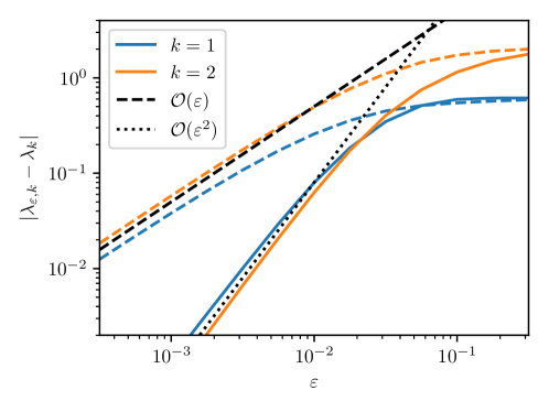
An empirical comparison of the bias errors for the standard and Sinkhorn normalisations on a $C^{2+\beta}$ sampling distribution is given in Figure 1, demonstrating the optimality of the bias error bounds, and the better convergence of the Sinkhorn normalisation for $\alpha=\tfrac{1}{2}$.

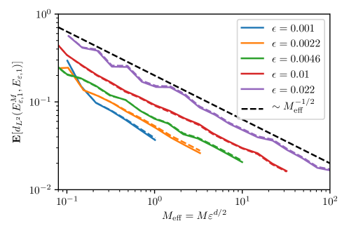
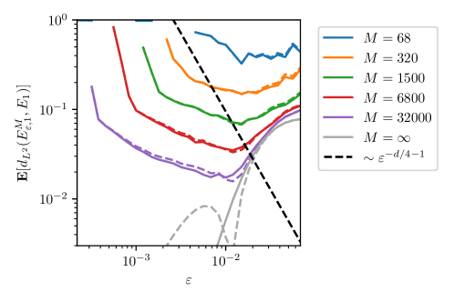
The empirical behaviour of variance errors for a three-dimensional example is given in Figure 2. Here the variance error in the spectral data appears to have the central limit theorem convergence in the sample size $M$ that we have shown. However, this convergence occurs in the regime $M_{\mathrm{eff}}=M\varepsilon^{d/2}\gg 1$, i.e. up to log terms that $\delta\ll 1$: this regime is larger than that covered by our results, $\varepsilon^{-1}\delta\ll 1$. Furthermore, the dependence on the timestep $\varepsilon$ appears to be more gentle than our results would suggest: as $\varepsilon$ is decreased with $M_{\mathrm{eff}}$ fixed, the variance error in fact appears to decrease rather than increasing as $\mathcal{O}(\varepsilon^{-1})$. This is in accordance with previous observations that spectral estimates have better convergence than the pointwise estimates that our results match up to (Trillos et al. 2019, Calder & Trillos 2019).

Figure 1: Bias error in eigenvalues for $C^{2.2^{-}}$ function density $\rho(x)=1+\tfrac{1-3^{-2.2}}{2}\sum_{j=1}^{\infty}3^{-2.2j}\cos(3^{j}\cdot 2\pi x)$ on $\mathbb{D}=\mathbb{R}/\mathbb{Z}$ using a Sinkhorn normalisation (solid lines) and $\alpha=\tfrac{1}{2}$ standard normalisation (dashed lines). A Fourier operator discretisation with $2001$ modes was used to compute the spectrum of the generator $\mathcal{L}$ and discrete-time approximations $\mathcal{P}_{\varepsilon},\check{\mathcal{P}}_{\varepsilon,1/2}$.

Figure 2: $L^{2}(\rho^{M})$ error in diffusion maps estimates of eigenspace $E_{1}$ for function density $\rho(x,y,z)\propto e^{\cos 4\pi x+f(y)+f(z)}$ where $f(x)=0.4\cos 2\pi x+0.12\sin 4\pi x$ on $\mathbb{D}=(\mathbb{R}/\mathbb{Z})^{3}$. Sinkhorn normalisation (solid lines) and $\alpha=\tfrac{1}{2}$ standard normalisation (dashed lines) are compared. At top, the variance error plotted against local sample size $M_{\mathrm{eff}}$ for different $\varepsilon$; at bottom the combined bias and variance error are plotted against timestep $\varepsilon$ for different sample sizes $M$. Expectations were computed using $30$ samples each. An adaptive Fourier discretisation (Olver 2019) was used to approximate the eigenfunctions of the generator $\mathcal{L}$ and of the continuum semigroup approximations $\mathcal{P}_{\varepsilon},\check{\mathcal{P}}_{\varepsilon,1/2}$.

Rather than the semigroup, one is often interested in approximating the Laplace-Beltrami operator $\mathcal{L}$ itself via the (possibly weighted) graph Laplacian $\varepsilon^{-1}(P-I)$: as an operator, we are thus interested in

$$\mathcal{L}^{(M)}_{\varepsilon}:=\varepsilon^{-1}(\mathcal{P}^{(M)}_{\varepsilon}-I),$$

and similarly for the standard weights. The eigenfunctions of these operators are the same as that of the respective $\mathcal{P}^{(M)}_{\varepsilon}$, thus with the same convergence. On the other hand, if we let the eigenvalues of the generator $\mathcal{L}^{(M)}_{\varepsilon}$ be

(27) $$-\tilde{\lambda}_{k,\varepsilon}^{(M)}=\varepsilon^{-1}(e^{-\lambda_{k,\varepsilon}^{(M)}}-1),$$

and similarly for standard weights

(28) $$-\check{\tilde{\lambda}}_{k,\alpha,\varepsilon}^{(M)}=\varepsilon^{-1}(e^{-\check{\lambda}_{k,\alpha,\varepsilon}^{(M)}}-1),$$

then we also have convergence of eigenvalues.

Corollary 3.4 (Eigendata of the graph Laplacian).

For all $\alpha\in[0,1]$ and $\lambda_{*}>0$ there exist constants ${{C}}_{3},{{C}}_{6},\check{{C}}_{3},\check{{C}}_{6}$ such that

1. The eigenspaces of the graph Laplacians $\mathcal{L}^{(M)}_{\varepsilon}$ are those of the respective semigroup approximations $\mathcal{P}^{(M)}_{\varepsilon}$ given in Theorems 3.2 and 3.3.

2. If $\rho\in C^{3/2+\beta}$ and $\varepsilon+\varepsilon^{-1}\delta<\check{{C}}_{3}$, then for $-\check{\lambda}_{k,\alpha}\geq-\lambda_{*}$ we have convergence of eigenvalues for the standard weights

   $$|\tilde{\check{\lambda}}_{k,\varepsilon,\alpha}-\check{\lambda}_{k,\alpha}| \leq\check{{C}}_{6}\varepsilon,$$

   $$|\tilde{\check{\lambda}}_{k,\varepsilon,\alpha}^{M}-\check{\lambda}_{k,\alpha}| \leq\check{{C}}_{6}(\varepsilon+\varepsilon^{-1}\delta).$$

3. If $\rho\in C^{2+\beta}$ and $\varepsilon^{2}+\varepsilon^{-1}\delta<{{C}}_{3}$, then for $-\lambda_{k}\geq-\lambda_{*}$ we have convergence of eigenvalues for the Sinkhorn weights

   $$|\tilde{\lambda}_{k,\varepsilon}-\lambda_{k}| \leq{{C}}_{6}\varepsilon,$$

   $$|\tilde{\lambda}_{k,\varepsilon}^{M}-\lambda_{k}| \leq{{C}}_{6}(\varepsilon+\varepsilon^{-1}\delta).$$

Note however that for purely linear-algebraic reasons the improvement in the bias error to $\mathcal{O}(\varepsilon^{2})$ for Sinkhorn weights is lost.

Our proof of the main results rely on bounds of the deviations of (powers of) our discretised half-step operators $\mathcal{G}^{(M)}_{\varepsilon},\mathcal{H}^{(M)}_{\varepsilon}$ from their respective limits.

Thus for the Sinkhorn weights, the bias error is bounded according to the following theorem:

Theorem 3.5.

Suppose $\rho\in W^{s,\infty},\,s>2$, and let $S_{\varepsilon}(t_{1},t_{0})$ be the solution operator of the PDE

(29) $$\partial_{t}\phi^{t}=\mathcal{L}\phi^{t}+\nabla\hat{w}^{t}_{\varepsilon}\cdot\nabla\phi^{t},$$

where we define $\hat{w}^{t}_{\varepsilon}:=\log(\mathcal{K}_{t}U_{\varepsilon})-\tfrac{1}{2}\log\rho$ for $t\in[0,\varepsilon)$ and extend $\varepsilon$-periodically.

Then

$$\mathcal{G}_{\varepsilon} =S_{\varepsilon}(\varepsilon,\tfrac{1}{2}\varepsilon)$$

$$\mathcal{H}_{\varepsilon} =S_{\varepsilon}(\tfrac{1}{2}\varepsilon,0)$$

$$\mathcal{P}_{\varepsilon} =S_{\varepsilon}(\varepsilon,0)$$

$$\mathcal{Q}_{\varepsilon,n} =S_{\varepsilon}((n+\tfrac{1}{2})\varepsilon,\tfrac{1}{2}\varepsilon).$$

Furthermore, for all $T>0$ and $\beta\in(0,\min\{s-2,1\})$ there exists a constant ${{C}}_{7,T,\beta}$ such that for all $0\leq t_{1}-t_{0}\leq T$ and $\varepsilon\leq\varepsilon_{0}$,

(30) $$\|S_{\varepsilon}(t_{1},t_{0})-e^{(t_{1}-t_{0})\mathcal{L}}\|_{C^{3+\beta}\to C^{0}}\leq{{C}}_{7,T,\beta}\varepsilon^{2}.$$

If the sampling density $\rho$ has higher regularity, we have the stronger result, which follows from a simplification of the proof of Theorem 3.5 and implies an $\mathcal{O}(\varepsilon^{2})$ pointwise bias error of the Sinkhorn-weighted graph Laplacian:

Proposition 3.6.

Suppose $\rho\in W^{s,\infty}$ for $s>4$. Then for all $\beta\in(0,1)$ there exists a constant ${{C}}_{8,\beta}$ such that for all $t\in\mathbb{R}$, $\varepsilon\leq\varepsilon_{0}$,

$$\|S_{\varepsilon}(t+\varepsilon,t)-e^{\varepsilon\mathcal{L}}\|_{C^{3+\beta}\to C^{0}}\leq{{C}}_{8,\beta}\varepsilon^{3}.$$

This is the best possible asymptotic rate of convergence to the semigroup for operators of the form $V_{\varepsilon}\mathcal{K}_{\varepsilon}U_{\varepsilon}$ for all non-uniform distributions $\rho$ (see Remark 7.2).

Bounds on the variance error proceed from Theorem 3.1. In particular, we have the following result on the convergence of the operator $\mathcal{K}^{M}_{\varepsilon}$ (an interpolation of the kernel matrix $K$) to its continuum limit:

Theorem 3.7.

Let $\zeta=Z_{0}\varepsilon^{1/2}$. Then

$$\left\|\mathcal{K}^{M}_{\varepsilon}-\mathcal{K}_{\varepsilon}\right\|_{H^{\infty}(\mathbb{D}_{\zeta})}\leq e^{2dZ_{0}^{2}}\delta.$$

Note here that the imaginary-direction thickness $\zeta$ of the domain of the Hardy space $H^{\infty}(\mathbb{D}_{\zeta})$ scales proportionally with the $\mathcal{O}(\varepsilon^{1/2})$ bandwidth of the kernel. A useful consequence of this is that it is also possible to bound the error of the $k$th derivative of the spatial discretisation, with a penalty in the error of $\mathcal{O}(\varepsilon^{-k/2})$.

As a consequence of Theorem 3.7, we also have operator convergence of the normalised operator $\mathcal{P}^{M}_{\varepsilon}$, which interpolates the matrix $P$, as well as the various auxiliary operators:

Theorem 3.8.

There exist constants $Z_{0},{{C}}_{9},{{C}}_{10}$ such that if $\zeta=Z_{0}\varepsilon^{1/2}$ and $\delta\leq{{C}}_{9}$ then for all $\varepsilon\leq\varepsilon_{0}$ and $n\in\mathbb{N}$,

$$\|\mathcal{P}^{M}_{\varepsilon}-\mathcal{P}_{\varepsilon}\|_{\zeta},\,\|\mathcal{G}^{M}_{\varepsilon}-\mathcal{G}_{\varepsilon}\|_{0\to\zeta},\,\|\mathcal{H}^{M}_{\varepsilon}-\mathcal{H}_{\varepsilon}\|_{\zeta\to 0}\leq{{C}}_{10}\delta,$$

and

$$\|\mathcal{Q}^{M}_{\varepsilon,n}-\mathcal{Q}_{\varepsilon,n}\|_{0}\leq{{C}}_{10}\delta n.$$

4 Numerical computation of Sinkhorn weights

While the use of Sinkhorn weights gives improved convergence in spectral data, it is necessary to calculate them iteratively: the usual Sinkhorn iteration is known to converge quite slowly in other problems, and indeed substantial efforts have been dedicated to finding ways to accelerate the convergence (Thibault et al. 2017, Altschuler et al. 2017, Feydy et al. 2019, Peyré & Cuturi 2019).

However, in our case the extra numerical work necessary to obtain the Sinkhorn weights is small, as in this section we will present a simple, general, well-conditioned algorithm to estimate the Sinkhorn weights that converges exponentially at a rate that is independent of the matrix input.

Let us first note that the traditional way that Sinkhorn weights are calculated is using so-called Sinkhorn iteration: for symmetric matrices this amounts to repeatedly iterating

$$u^{(n+1)}=1/(Ku^{(n)}),$$

which is interpolated as

(31) $$U^{(n+1)}=1/\mathcal{K}^{M}_{\varepsilon}[U^{(n)}].$$

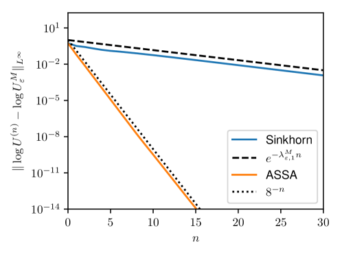
As $n\to\infty$, it is well-known that $U^{(n)}\to c^{(-1)^{n}}U^{M}_{\varepsilon}$ for some constant $c>0$ (Peyré & Cuturi 2019). The asymptotic rate of convergence can be bounded, since at the fixed point Sinkhorn iteration is a contraction by $\lambda^{M}_{\varepsilon,1}$, the second eigenvalue of the re-weighted operator $\mathcal{P}^{M}_{\varepsilon}$. This is because the Jacobian at the fixed point is conjugate to $-\mathcal{P}^{M}_{\varepsilon}$. However, from Theorem 3.3, the spectral gap $1-\lambda^{M}_{\varepsilon,1}=\mathcal{O}(\varepsilon)$, so $\mathcal{O}(\varepsilon^{-1})$ iterates are needed to estimate the Sinkhorn weights to a given tolerance.

0:  Unweighted kernel matrix $K$, timestep $\varepsilon$, eigendata error tolerance $\tau$

0:  Estimated Sinkhorn weight vector $u$ with log-$L^{\infty}$ error less than $\varepsilon\tau$

  $u\leftarrow 1/\sqrt{K\mathbf{1}}$

  repeat

     $u_{o}\leftarrow u$

     $v\leftarrow 1/(Ku_{o})$

     $u\leftarrow\sqrt{v/(Kv)}$

  until $\|\log(u_{o}/u)\|_{\ell_{2}}\leq\varepsilon\tau$

Algorithm 1 Accelerated symmetric Sinkhorn algorithm (ASSA)

To improve this, we propose an accelerated symmetric Sinkhorn algorithm (ASSA, Algorithm 1), which harnesses the symmetry and positive definiteness of the iteration problem to accelerate the local convergence rate to $\mathcal{O}(8^{-n})$, as well as automatically removing the constant $c$. An iteration step of ASSA involves taking two successive Sinkhorn iterates (c.f. $(\ref{eq:SinkhornIteration})$), followed by a geometric mean of the two steps. This algorithm was first noted as a heuristic by Marshall & Coifman (2019).

We can write this in the case of a kernel operator $\mathcal{K}$ as

(32) $$U^{(n)}_{a} =1/\mathcal{K}[U^{(n)}]$$

(33) $$U^{(n)}_{b} =1/\mathcal{K}[U^{(n)}_{a}]$$

(34) $$U^{(n+1)} =\sqrt{U^{(n)}_{a}U^{(n)}_{b}}.$$

Because the Jacobian of a Sinkhorn iteration step $(\ref{eq:SinkhornIteration})$ around the fixed point $U$ is conjugate to $-\mathcal{P}:=-U\mathcal{K}U$, the Jacobian of the ASSA step is conjugate to $-\tfrac{1}{2}\mathcal{P}(I-\mathcal{P})$. In our case $\mathcal{P}=\mathcal{P}^{M}_{\varepsilon}$ is a self-adjoint, positive definite Markov operator on $L^{2}(\rho^{M})$, so its spectrum is contained in $[0,1]$ and so the spectrum of the Jacobian is contained in $[-\tfrac{1}{8},0]$, leading to $\mathcal{O}(8^{-n})$ local rate of contraction. The geometric mean step additionally removes the constant $c$ that is an artefact of the usual Sinkhorn algorithm. In Theorem 4.1, whose proof is in Appendix A, we show in a general setting that Algorithm 1 is guaranteed to converge for any positive initial guess, and, assuming a good initial guess, converges at the $\mathcal{O}(8^{-n})$ rate with a valid stopping condition. Around $40$ ASSA iterates are typically sufficient to obtain an estimate of the Sinkhorn weight accurate to double floating point.

Theorem 4.1.

Suppose $\mu$ is a measure and $\mathcal{K}$ a positive operator that is bounded, positive semi-definite and self-adjoint on $L^{2}(\mu)$ and bounded on $L^{\infty}(\mu)$.

Let $U$ solve the Sinkhorn problem for this operator, and let $U^{(n)}$ be the $n$th iterate of the accelerated symmetric Sinkhorn algorithm $(\ref{eq:ASSA1}-\ref{eq:ASSA3})$ with $U^{(0)}>0$ . Then

1. (Global convergence) For all $n\geq 0$ and $U^{(0)}>0$,

   $$\|\log U^{(n)}-\log U\|_{L^{\infty}(\mu)}\leq 2\left(\theta\tfrac{1+\theta}{2}\right)^{n}\|\log U^{(0)}-\log U\|_{L^{\infty}(\mu)},$$

   where $\theta<1$ is the worst-case contraction rate of standard Sinkhorn iteration, given in the proof $(\ref{eq:ConeContractionRate})$.

2. (Local convergence rate) If $\|\log U^{(0)}-\log U\|_{L^{\infty}(\mu)}\leq k<0.1$, then if $k^{\prime\prime}:=ke^{4k}(2+\tfrac{1}{2}ke^{4k})<\tfrac{3}{8}$, the faster convergence holds

   $$\|\log U^{(n)}-\log U\|_{L^{2}(\mu)}\leq(\tfrac{1}{8}+k^{\prime\prime})^{n}\|\log U^{(0)}-\log U\|_{L^{2}(\mu)}.$$

3. (Stopping condition) Under the conditions of part (b),

   $$\|\log U^{(n)}-\log U\|_{L^{2}(\mu)}\leq(1-(\tfrac{1}{8}+k^{\prime\prime})^{-1})^{-1}\|\log U^{(n)}-\log U^{(n-1)}\|_{L^{2}(\mu)}.$$

Proposition 4.2.

The empirical measure $\rho^{(M)}$ and kernel operator $\mathcal{K}^{(M)}_{\varepsilon}$ respectively satisfy the conditions for Theorem 4.1.

Note that when $\mu$ is a discrete measure (e.g. $\mu=\rho^{M}$) we can recover bounds on the $L^{\infty}$ norm using norm equivalence:

$$\|\cdot\|_{L^{\infty}(\rho^{M})}\leq M^{-1/2}\|\cdot\|_{L^{2}(\rho^{M})}.$$

It is also possible to relax the positive semi-definiteness constraint on the kernel operator $\mathcal{K}$, as long as the negative spectrum of the weighted operator $\mathcal{P}$ is far away from $-1$.

Because the only steps in ASSA are standard Sinkhorn iteration and a geometric mean, ASSA is very well-conditioned, and can be expected to perform well in more general circumstances, including for samples on curved manifolds and from distributions with non-compact support: in Figure 3 fast convergence of ASSA is shown for a Gaussian sampling distribution.

As an initial value for iteration we use the standard $\alpha=\tfrac{1}{2}$ right-hand weight $U^{(0)}=(\mathcal{K}^{M}_{\varepsilon}1)^{-1/2}$. According to the following proposition, when $\varepsilon,\delta\ll 1$, this guess should be close enough to the Sinkhorn weight that the fast local convergence rate takes hold immediately.

Proposition 4.3 (ASSA initialisation).

There exist constants ${{C}}_{11},{{C}}_{12}$ independent of $M,\varepsilon$ such that if $\delta<{{C}}_{11}$ and $\varepsilon\leq\varepsilon_{0}$, then

$$\|\log(\mathcal{K}^{M}_{\varepsilon}1)^{-1/2}-\log U^{M}_{\varepsilon}\|_{L^{\infty}(\rho^{M})}\leq{{C}}_{12}(\delta+\varepsilon),$$

where $(\mathcal{K}^{M}_{\varepsilon}1)^{-1/2}$ is the initial condition for ASSA.

Figure 3: Convergence of standard Sinkhorn iteration (blue) and ASSA (orange) for an $M=3000$ sample from the standard normal distribution in dimension 3 with kernel parameter $\varepsilon=0.5$.

These results are proven in Appendix A.

5 Function space results

Before we study the $\varepsilon\to 0$ operator limit, we state some useful results in functional analysis.

Recall from Section 2.2 that we defined scales of fractional Sobolev spaces $W^{s,p}$ of functions $\phi$ for which $J^{s}\phi\in L^{p}$, where the sectorial Bessel operator $J:=I-\Delta$.

A sufficient condition for a Banach space operator $\mathcal{A}:B\to B$ to be sectorial is that its spectrum is confined to a left open half-plane and there exists $C<\infty$ such that for $\lambda$ in the complement of this half-plane

$$\|(\lambda+\mathcal{A})^{-1}\|_{B}\leq C|\lambda|^{-1}.$$

The operators $J$ and $\tilde{J}:=I-2\mathcal{L}$ are both sectorial on $L^{p}=W^{0,p}$ provided that our measure density $\rho\in C^{1+\beta}$ (Haase 2006). The Bessel operator $J$ is also sectorial on $W^{s,p}$ for all positive $s$.

From Theorem 1.4.8 in Henry (2006) and using that $\nabla$ is bounded as an operator from $W^{s+1,p}\to W^{s,p}$, we have by induction that $\tilde{J}=I-2L$ is a sectorial operator on $W^{r,p},\,r\leq s,\,p>1$ and that for $\beta\in[0,1]$, $\tilde{J}^{\beta/2}$ is bounded as an operator $W^{r+\beta,p}\to W^{r,p},r\leq s$. The condition for this to hold is that multiplication by $J^{1/2}\log\rho$ is bounded on $W^{r,p},r\leq s$: this is assured by the Leibniz rule for fractional derivatives $J^{\beta/2}$ (Bourgain & Li 2014, Li 2019), provided $\rho\in W^{s,p}$ and $s\geq 1$.

Standard results, for instance in Chapter 1 of Henry (2006), and the aforementioned Leibniz rule, give the following, as well as analogues for $\check{\mathcal{L}}_{\alpha}$:

Proposition 5.1.

Suppose that $\rho\in W^{s,\infty}$ for $s\geq 1$. Then for all $p\in(1,\infty]$:

• There exist constants $K^{\nabla}_{p}$ such that for all $r\geq 0$

  $$\|\nabla\|_{W^{r+1,p}\to W^{r,p}},\|\nabla\cdot\|_{W^{r+1,p}\to W^{r,p}}\leq K^{\nabla}_{p};$$

• For all $0\leq q\leq r\leq s$ there exists a constant $K^{\times}_{p;r,s}$ such that for all $\phi\in W^{r,p},\psi\in W^{s,\infty}$,

  $$\|\phi\psi\|_{W^{r,p}}\leq K^{\times}_{p;q,r,s}\|\phi\|_{W^{r,p}}\|\phi\|_{W^{s,\infty}};$$

• For all $r<s-2$, there exists $K_{p;r}$ such that

  $$\|\mathcal{L}\|_{W^{r+2,p}\to W^{r,p}}\leq K_{p;r};$$

• For all $s<k+\beta$, $\beta\in(0,1)$, there exists $K^{C}_{k+\beta,s}$ such that the norm of the inclusion map $C^{k+\beta}\to W^{s,\infty}$ is bounded by $K^{C}_{k+\beta,s}$.

• For all $q\leq r\leq s$ and all $T>0$ there exists $K^{T}_{p;q,r}$ such that for $t\in[0,T]$

  $$\|e^{t\mathcal{L}}\|_{W^{q,\infty}\to W^{r,\infty}}\leq t^{-(r-q)/2}K^{T}_{p;q,r};$$

• There exists $a>0$ such that for all $q\leq r\leq s$ and all $T>0$ there exists $\tilde{K}^{T}_{p;q,r}$ such that for $t\in[0,T]$

  $$\|e^{t\mathcal{L}}|_{Z\cap W^{q,\infty}}\|_{W^{q,\infty}\to W^{r,\infty}}\leq t^{-(r-q)/2}e^{-at}\tilde{K}^{T}_{p;q,r},$$

  where the $\mathcal{L}$-invariant subspace

  (35) $$Z=\left\{\phi\in L^{\infty}:\int_{\mathbb{D}}\phi\,\rho\,{\rm d}x=0\right\}.$$

6 Convergence of Sinkhorn weights as $\varepsilon\to 0$

Our convergence analysis requires an understanding the behaviour of the continuum limit Sinkhorn weights $U_{\varepsilon}$. These satisfy the equation $(\ref{eq:SinkhornProblem})$, which in this section we will find useful to formulate as

(36) $$U_{\varepsilon}^{-1}=\mathcal{C}_{\varepsilon}(\sigma^{2}U_{\varepsilon}),$$

where $\mathcal{C}_{\varepsilon}$ is convolution with the Gaussian kernel $g_{\varepsilon,L}$ and $\sigma^{2}:=\rho$. We expect $U_{\varepsilon}$ to converge to $\sigma^{-1}=\rho^{-1/2}$ as $\varepsilon\to 0$, but because the kernel $g_{\varepsilon,L}$ becomes singular as $\varepsilon\to 0$ this is not trivial.

We consider this problem by formulating $U_{\varepsilon}$ as the fixed point (up to constant scaling) of the Sinkhorn iteration:

(37) $$U^{(n+1)} =1/(\mathcal{C}_{\varepsilon}(\sigma^{2}U^{(n)}))$$

Since for fixed $\varepsilon>0$ the operator $\mathcal{C}_{\varepsilon}\sigma^{2}$ is uniformly positive, Sinkhorn iteration is a contraction on the cone of positive functions and thus for all initial conditions $U_{0}>0$ the convergence holds (Sinkhorn 1964)

$$U^{(2n)}\to cU_{\varepsilon},U^{(2n+1)}\to c^{-1}U_{\varepsilon}$$

for some $c>0$ depending on $U^{(0)}$. Note that while the iteration $(\ref{eq:SinkhornIter1})$ in the $\varepsilon\to 0$ limit has 2-periodic dynamics for all initial conditions, we do recover a fixed point $U_{0}=\rho^{-1/2}=\sigma^{-1}$ that is the solution of the Sinkhorn problem $(\ref{eq:SinkhornProblemAgain})$ for $\varepsilon=0$.

Motivated by the log-space formulation of cone metrics we set

$$w^{n\varepsilon} =(-1)^{n}\log\sigma U^{(n)},$$

so that

(38) $$w^{(2n+1)\varepsilon} =\mathcal{N}_{\varepsilon}w^{2n\varepsilon}$$

(39) $$w^{(2n+2)\varepsilon} =-\mathcal{N}_{\varepsilon}(-w^{2n\varepsilon}),$$

where the nonlinear semigroup $(\mathcal{N}_{t})_{t\geq 0}$ is given by

$$\mathcal{N}_{t}\phi=\log(\sigma^{-1}\mathcal{C}_{t}(\sigma e^{\phi})).$$

Using that $\frac{{\rm d}}{{\rm d}t}\mathcal{C}_{t}=\tfrac{1}{2}\Delta\mathcal{C}_{t}$ it is straightforward to show that the infinitesimal generator of $\mathcal{N}_{t}$ is given by

$$\left.\frac{{\rm d}}{{\rm d}t}\mathcal{N}_{t}\phi\right|_{t=0}=\tfrac{1}{2}\Delta\phi+\tfrac{1}{2}|\nabla\phi|^{2}+\frac{\nabla\sigma}{\sigma}\cdot\nabla\phi+\frac{\Delta\sigma}{2\sigma}.$$

By using $\mathcal{N}_{t}$ to interpolate $(\ref{eq:SinkhornLogDiscrete1}-\ref{eq:SinkhornLogDiscrete2})$ in time, we can thus write Sinkhorn iteration as a nonlinear PDE

(40) $$\partial_{t}w^{t}=\mathcal{L}w^{t}+(-1)^{\lfloor\varepsilon^{-1}t\rfloor}\left(\tfrac{1}{2}|\nabla w^{t}|^{2}+\frac{\Delta\sigma}{2\sigma}\right).$$

This reformulation can be seen as the reverse of the Cole-Hopf transformation (Evans 1998).

Now, the the PDE $(\ref{eq:SinkhornPDE})$ can be decomposed as a sum of an autonomous linear part, in fact the limiting generator of the diffusion maps problem $\mathcal{L}$, with a non-autonomous, rapidly oscillating nonlinear part that has time integral zero. Consequently, we can apply averaging results to this system as $\varepsilon\to 0$. This will give us convergence of $w^{t}$ and thus $U_{\varepsilon}$:

Theorem 6.1.

Suppose $\rho\in W^{s,\infty},\,s\geq 2$.

Then the PDE $(\ref{eq:SinkhornPDE})$ has a unique limit cycle $w_{\varepsilon}^{t}$ with $w_{\varepsilon}^{t+\varepsilon}=-w_{\varepsilon}^{t}$ and $w_{\varepsilon}^{0}=\log\rho^{1/2}+\log U_{\varepsilon}$.

Furthermore for all $0\leq r<s+1$,

$$\lim_{\varepsilon\to 0}\sup_{t}\|w_{\varepsilon}^{t}\|_{W^{r,\infty}}=0,$$

and

$$\lim_{\varepsilon\to 0}\|\log U_{\varepsilon}-\log\rho^{-1/2}\|_{W^{r,\infty}}=0.$$

This has the following immediate corollary:

Corollary 6.2.

Suppose $\rho\in W^{s,\infty},\,s\geq 2$. Then there exists a constant ${{C}}_{22}$ such that for all $\varepsilon\leq\varepsilon_{0}$

$$\sup_{\varepsilon\leq\varepsilon_{0}}\|U_{\varepsilon}\|_{C^{3}}\leq{{C}}_{22}<\infty$$

and for all $r<s+1$ a constant ${{C}}_{23,r}$ such that that for all $\varepsilon\leq\varepsilon_{0}$

$$\sup_{\varepsilon\leq\varepsilon_{0}}\sup_{t}\|w_{\varepsilon}^{t}\|_{W^{r,\infty}}\leq{{C}}_{23,r}<\infty.$$

The uniform bounds on the ($2\varepsilon$-periodic) limit cycle $w^{t}_{\varepsilon}$ are of particular use to us, because $w^{t}_{\varepsilon}=(-1)^{\lfloor t/\varepsilon\rfloor}w^{t}_{\varepsilon}$: that is, up to a periodic change of sign, it is the same as the $\varepsilon$-periodic drift error term in the time discretisation of diffusion maps $(\ref{eq:SDMPDE})$.

Remark 6.3.

By applying instead Theorem 1.1 of Ilyin (1998), one can show that as $\varepsilon\to 0$, the solution of the Sinkhorn iteration PDE $(\ref{eq:SinkhornPDE})$, $w^{t}$, converges to an averaging limit

$$\partial_{t}\bar{w}^{t}=\mathcal{L}\bar{w}^{t}$$

over finite time scales (c.f. the Monge-Ampere PDE derived for non-symmetric Sinkhorn iteration in Berman (2017)). As a result, one recovers the asymptotic rate of (standard) Sinkhorn iteration

$$\lim_{n\to\infty}\frac{-\log\|U^{(n)}-U_{\varepsilon}\|}{n}=-\lambda_{1}\varepsilon,$$

where $-\lambda_{1}$ is the first non-zero eigenvalue of the Langevin dynamics $\mathcal{L}$.

Proof 6.4 (Proof of Theorem 6.1).

This amounts to checking the conditions of Theorem 1.2 of Ilyin (1998). Due to the invariance of constant functions under Sinkhorn iteration we will project our PDE $(\ref{eq:SinkhornPDE})$ onto the subspace of zero mean functions $Z$ defined in $(\ref{eq:ZeroSpace})$. We thus consider

(41) $$\partial_{t}w^{t}=\mathcal{L}w^{t}+\mathcal{F}(w^{t},\varepsilon^{-1}t)+\mathcal{X}(\varepsilon^{-1}t),$$

where

$$\mathcal{F}(\phi,\tau) =(-1)^{\lfloor\tau\rfloor}\tfrac{1}{2}(I-\mathcal{Z})\left(|\nabla\phi|^{2}\right)$$

$$\mathcal{X}(\tau) =(-1)^{\lfloor\tau\rfloor}(I-\mathcal{Z})\left(\frac{\Delta\sigma}{2\sigma}\right),$$

and the projection operator

$$(\mathcal{Z}\phi)(x):=\int_{\mathbb{D}}\phi(y)\rho(y)\,{\rm d}y.$$

Suppose $r\geq s-1$ (the result will then follow immediately for $r<s-1$). Set Banach spaces $E=W^{r,\infty}\cap Z,F=W^{r-1,\infty}\cap Z,X=W^{s-2,\infty}\cap Z$ and $\mathcal{E}=Z$.

Proposition 5.1 implies the various conditions on the linear operator $\mathcal{L}$ and the averaged semigroup $e^{\mathcal{L}t}$ required for Theorem 1.2 of Ilyin (1998). We also have that the nonlinear part $\mathcal{F}:E\times\mathbb{R}\to F$ is Lipschitz on bounded subsets of $E$ and the driver $\mathcal{X}$ has range in $X$. Both are locally integrable over $\tau$. As a result, we have that the attractor of $(\ref{eq:SinkhornPDEProj})$ converges in the strong space $E$ uniformly to the attractor of $\partial_{t}w^{t}=\mathcal{L}w^{t}$ in $E$, i.e. zero. In other words, if $\{w_{\varepsilon}^{t,\mathcal{Z}}\}_{t\in\mathbb{R}}$ is this attractor (which by the convergence of Sinkhorn iteration is necessarily a unique limit cycle), then

$$\lim_{\varepsilon\to 0}\sup_{t}\|w_{\varepsilon}^{t,\mathcal{Z}}\|_{E}=0.$$

If we let $w_{\varepsilon}^{t}$ be the solution of the unprojected PDE $(\ref{eq:SinkhornPDE})$ corresponding to the true Sinkhorn weights with $w_{\varepsilon}^{n\varepsilon}=(-1)^{n}\log\sigma U_{\varepsilon}$, then for all $t$ one has $w_{\varepsilon}^{t+\varepsilon}=-w_{\varepsilon}^{t}$; furthermore if $w_{\varepsilon}^{t,\mathcal{Z}}$ is the attractor (necessarily a limit cycle) of the projected PDE $(\ref{eq:SinkhornPDEProj})$ then

$$w_{\varepsilon}^{t}-w_{\varepsilon}^{t,\mathcal{Z}}=\mathcal{Z}w_{\varepsilon}^{t}=\int_{\mathbb{D}}w_{\varepsilon}^{t}\,\rho\,{\rm d}y.$$

From $(\ref{eq:SinkhornPDE})$ and using that $\nabla w_{\varepsilon}^{t}=\nabla w_{\varepsilon}^{t,\mathcal{Z}}$ we find that

$$\sup_{\varepsilon\leq\varepsilon_{0}}\left\|\partial_{t}\mathcal{Z}w_{\varepsilon}^{t}\right\|=\sup_{\varepsilon\leq\varepsilon_{0}}\left|\int_{\mathbb{D}}\left(\tfrac{1}{2}|\nabla w_{t,\mathcal{Z}}|^{2}+\frac{\Delta\sigma}{2\sigma}\right)\,\rho\,{\rm d}x\right|<\infty.$$

Then using that $\mathcal{Z}w_{\varepsilon}^{t+\varepsilon}=\tfrac{1}{2}(\mathcal{Z}w_{\varepsilon}^{t+\varepsilon}-\mathcal{Z}w_{\varepsilon}^{t})$ implies that

$$\lim_{\varepsilon\to 0}\sup_{t}\|w_{\varepsilon}^{t}-w_{\varepsilon}^{t,\mathcal{Z}}\|_{W^{r,\infty}}\to 0,$$

giving us what is required.

Because $w^{t}_{\varepsilon}$ is, up to a time-varying change of sign, the drift term in the temporally-discretised PDE $(\ref{eq:SDMPDE})$, we will find it useful to make some more specific estimates on $w^{t}_{\varepsilon}$ to prove the operator convergence in the next section. In particular, we will show that $w^{t}_{\varepsilon}=\mathcal{O}(\varepsilon)$, and that $w_{\varepsilon}^{t}$ is, up to $\mathcal{O}(\varepsilon^{2})$, symmetric in time.

Lemma 6.5.

Suppose $\rho\in W^{s,\infty}$, $s>2$ and $w^{t}_{\varepsilon}$ is as in Theorem 6.1. Then for all $r\in[2,s+1)$ there exist ${{C}}_{24,r},{{C}}_{25,r}$ such that for all $\varepsilon\leq\varepsilon_{0}$, $t\in[0,\varepsilon]$

(42) $$\|w^{t}_{\varepsilon}\|_{W^{r-2,\infty}}\leq\tfrac{1}{2}{{C}}_{25,r}\varepsilon$$

and

(43) $$\|J^{-r^{*}/2}(w^{t}_{\varepsilon}+w^{\varepsilon-t}_{\varepsilon})\|_{W^{r-4+{r^{*}},\infty}}\leq{{C}}_{24,r}\varepsilon^{2},$$

where $r^{*}=\max\{4-r,0\}$.

Proof 6.6 (Proof of Lemma 6.5).

Making use of Corollary 6.2 and Proposition 5.1, we have that

$$\|\partial_{t}w^{t}_{\varepsilon}\|_{W^{r-2,\infty}}\leq\tfrac{1}{2}K_{\infty;r-2}{{C}}_{23,r}+K^{\times}_{\infty;,r-2,r-1,r-1}(K^{\nabla}_{\infty}{{C}}_{23,r-1})^{2}+\left\|\frac{\Delta\rho^{1/2}}{2\rho^{1/2}}\right\|_{W^{r-2,\infty}}=:{{C}}_{25,r}.$$

From Theorem 6.1 we have that $w^{t}_{\varepsilon}=-w^{t-\varepsilon}_{\varepsilon}$, and so as a result

$$\sup_{t\in[0,\varepsilon]}\|w^{t}_{\varepsilon}\|_{W^{r-2,\infty}}=\sup_{t\in[0,\varepsilon]}\tfrac{1}{2}\|w^{t}_{\varepsilon}-w^{t-\varepsilon}_{\varepsilon}\|_{W^{r-2,\infty}}\leq\tfrac{1}{2}{{C}}_{25,r}\varepsilon,$$

as required for $(\ref{eq:WBound})$.

To obtain $(\ref{eq:WSymBound})$, we will want to take the second derivative in time: however, for $r\in(2,4)$ we do not have enough regularity in our function spaces to do that, so we will introduce an inverse fractional derivative $J^{-r^{*}/2}$ to compensate. In particular, we have that for $t\in(0,\varepsilon)$,

$$\partial_{tt}J^{-r^{*}/2}w^{t} =\partial_{t}J^{-r^{*}/2}\partial_{t}w^{t}$$

$$=\tfrac{1}{2}\partial_{t}J^{-r^{*}/2}(-Jw^{t}+w^{t}+\nabla\log\rho\cdot\nabla w^{t}+\nabla\partial_{t}w^{t}\cdot\nabla w^{t}+\Delta\sigma/\sigma)$$

$$=-\tfrac{1}{2}J^{1-r^{*}/2}\partial_{t}w^{t}+\tfrac{1}{2}J^{-r^{*}/2}\partial_{t}w^{t}+\tfrac{1}{2}J^{-r^{*}/2}\nabla(\log\rho+2w^{t})\cdot\nabla\partial_{t}w^{t},$$

and as a result this second time derivative is uniformly bounded in $W^{r-4+r^{*},\infty}$:

$$\|\partial_{tt}J^{-r^{*}/2}w^{t}\|_{W^{r-4+r^{*},\infty}} \leq\tfrac{1}{2}{{C}}_{25,r}+\tfrac{1}{2}{{C}}_{23,r}+$$

$$\qquad\tfrac{1}{2}K^{\times}_{\infty;r-4+r^{*},r-1,r-3}(K^{\nabla}_{\infty})^{2}{{C}}_{25,r}(\|\log\rho\|_{W^{r-1,\infty}}+2{{C}}_{23,r-1})$$

$$=:\tfrac{1}{2}{{C}}_{24,r}.$$

Thus, by applying Taylor’s theorem,

(44) $$\left\|J^{-r^{*}/2}\left(w^{t}_{\varepsilon}+w^{\varepsilon-t}_{\varepsilon}-2w^{\varepsilon/2}_{\varepsilon}\right)\right\|_{W^{r-4+r^{*},\infty}}\leq\sup_{t\in[0,\varepsilon]}\|\partial_{tt}J^{-r^{*}/2}w^{t}\|_{W^{r-4+r^{*},\infty}}\varepsilon^{2}\leq\tfrac{1}{2}{{C}}_{24,r}\varepsilon^{2}.$$

Since $w^{0}_{\varepsilon}=-w^{\varepsilon}_{\varepsilon}$, by setting $t=0$ in $(\ref{eq:SinkhornWeightTaylor})$ we have

(45) $$\|2J^{-r^{*}/2}w^{\varepsilon/2}_{\varepsilon}\|_{W^{r-4+r^{*},\infty}}\leq\tfrac{1}{2}{{C}}_{24,r}\varepsilon^{2}.$$

Recombining this with $(\ref{eq:SinkhornWeightTaylor})$ we obtain the necessary result.

Remark 6.7.

Since from $(\ref{eq:SinkhornWeightMidpoint})$ we have for $s>4$ (i.e. $\rho\in C^{4+\beta}$) that

$$\|\mathcal{K}_{\varepsilon/2}U_{\varepsilon}-\rho^{1/2}\|_{L^{\infty}}=\mathcal{O}(\varepsilon^{2}),$$

the Sinkhorn problem can be used to perform second-order non-parametric estimation on the density $\rho$.

7 Deterministic convergence of operators

Recall from $(\ref{eq:SemigroupDeterministic})$ that the deterministic approximation to the semigroup is

$$\mathcal{P}_{\varepsilon}=U_{\varepsilon}\mathcal{K}_{\varepsilon}U_{\varepsilon}.$$

In this section, we will harness our results on the Sinkhorn weight $U_{\varepsilon}$ from the previous section to Theorem 3.5 on convergence of $\mathcal{P}_{\varepsilon}$ to the semigroup $e^{\varepsilon\mathcal{L}}$. Before this, we will make some remarks on the rate of convergence to the semigroup.

Remark 7.1.

For the Sinkhorn normalisation the bias error convergence is of second order in the timestep $\varepsilon$, unlike the first-order convergence for standard weights (c.f. Proposition 11.5). This is actually a result of the self-adjointness of the normalised operator.

To be more specific (and to outline the strategy of the proof of Theorem 3.5), we can write the action of $\mathcal{P}_{\varepsilon}$ as solving the PDE $(\ref{eq:SDMPDE})$, which we recall here,

$$\phi^{0} =\phi$$

(46) $$\partial_{t}\phi^{t} =\mathcal{L}\phi^{t}+\nabla\hat{w}^{t}_{\varepsilon}\cdot\nabla\phi^{t},$$

so that $\phi^{\varepsilon}=\mathcal{P}_{\varepsilon}\phi$, where recall that the discrepancy in drift compared with the semigroup is

$$\hat{w}^{t}_{\varepsilon}=\log(\mathcal{K}_{t}U_{\varepsilon})-\tfrac{1}{2}\log\rho,\,t\in[0,\varepsilon).$$

Note that because the Sinkhorn normalisation $(\ref{eq:SinkhornProblem})$ is required to be symmetric,

$$\hat{w}^{0}_{\varepsilon}=\log U_{\varepsilon}+\tfrac{1}{2}\log\rho=-\lim_{t\uparrow\varepsilon}\hat{w}^{t}_{\varepsilon}.$$

If $\phi,\rho,U_{\varepsilon}$ are of sufficiently high regularity, for small $\varepsilon$ we can average the PDE $(\ref{eq:GoodBecauseSymmetricPDE})$ over $t\in[0,\varepsilon]$:

$$\partial_{t}\phi^{t}\approx\mathcal{L}\phi^{t}+\nabla\left(\varepsilon^{-1}\int_{0}^{\varepsilon}\hat{w}^{t}_{\varepsilon}\,{\rm d}\tau\right)\cdot\nabla\phi^{t}.$$

The averaged drift can then be approximated using the trapezoidal rule with

$$\varepsilon^{-1}\int_{0}^{\varepsilon}\hat{w}_{\tau}^{\varepsilon}\,{\rm d}\tau =\tfrac{1}{2}(\hat{w}_{\varepsilon}^{0}+\lim_{t\uparrow\varepsilon}\hat{w}^{t}_{\varepsilon})+\mathcal{O}(\varepsilon^{2})=\mathcal{O}(\varepsilon^{2}).$$

As a result the operator $\mathcal{P}_{\varepsilon}$ should closely approximate $e^{\varepsilon\mathcal{L}}$, as required.

Remark 7.2.

The $\mathcal{O}(\varepsilon^{3})$ rate of convergence $\mathcal{P}_{\varepsilon}\to e^{\varepsilon\mathcal{L}}$ is in general the best possible for operators of the form $V_{\varepsilon}\mathcal{K}_{\varepsilon}U_{\varepsilon}$. We can best see this by comparing the re-weighted operators for $n=1$:

$$\sigma V_{\varepsilon}\mathcal{K}_{\varepsilon}U_{\varepsilon}\sigma^{-1}=V_{\varepsilon}\sigma e^{\varepsilon\tfrac{1}{2}\Delta}\sigma U_{\varepsilon}$$

and

$$\sigma e^{\varepsilon\mathcal{L}}\sigma^{-1}=e^{\varepsilon(\tfrac{1}{2}\Delta-\tfrac{1}{2}\sigma^{-1}\Delta\sigma)},$$

where $\sigma=\rho^{1/2}$. Taking a power series in $\varepsilon$ and writing each side in the form

$$\sum_{k\geq 0}\left(\tfrac{1}{2^{k}}\Delta^{k}+\sum_{j=0}^{k-1}\left(\beta_{j,k}\Delta^{j}+\nabla\beta_{j,k}\cdot\nabla\Delta^{j-1}\right)\right)\varepsilon^{k},$$

we see that for the $\beta_{k-1,k}$ coefficients to match it is necessary that

$$\left.\frac{\partial}{\partial\varepsilon}(V_{\varepsilon}+U_{\varepsilon})\right|_{\varepsilon=0}=-\frac{1}{2(k-1)!}\sigma^{-2}\Delta\sigma.$$

Unless $\Delta\sigma\equiv 0$, i.e. $\sigma=\rho^{1/2}$ is constant, then this can only hold simultaneously for $k=1,2$: an $\mathcal{O}(\varepsilon^{3})$ error between $e^{\varepsilon\mathcal{L}}$ and $V_{\varepsilon}\mathcal{K}_{\varepsilon}U_{\varepsilon}$ is thus the best possible (and hence we expect also an $\mathcal{O}(\varepsilon^{2})$ error for the spectral data).

To prove Theorem 3.5, we will require the following result:

Proposition 7.3.

Suppose $\rho\in W^{s,\infty},\,s>2$. Then for all $T>0$, $\beta\in(0,\min\{s-2,1\})$, there exists a constant ${{C}}_{31,T,\beta}$ such that for all $|t_{1}-t_{0}|\leq T$,

$$\|S_{\varepsilon}(t_{1},t_{0})\|_{C^{3+\beta}}\leq{{C}}_{31,T,\beta}.$$

Proof 7.4 (Proof of Proposition 7.3).

From Corollary 6.2, we have for all $r<s+1$ an $\varepsilon$-uniform bound on the $W^{r,\infty}$ norm of $w^{t}_{\varepsilon}=(-1)^{\lfloor t/\varepsilon\rfloor}\hat{w}^{t}_{\varepsilon}$. We therefore also have uniform in $\varepsilon$ bounds on the $C^{3+\beta}$ norm of $\tfrac{1}{2}\log\rho+\hat{w}^{t}_{\varepsilon}$ for $2+\beta<s$. We can thus apply Theorem 1.2 of Lorenzi (2000) to (29) to obtain relevant uniform bounds on $\|S_{\varepsilon}(t_{1},t_{0})\|_{C^{2+\beta}}$. By observing that (29) implies that

(47) $$\partial_{t}\partial_{x_{i}}\phi^{t}=\mathcal{L}\partial_{x_{i}}\phi^{t}+\nabla\partial_{x_{i}}(\tfrac{1}{2}\log\rho+w^{t})\cdot\nabla\phi^{t},$$

we can then re-apply Lorenzi (2000) to obtain bounds on $\|S_{\varepsilon}(t_{1},t_{0})\|_{C^{3+\beta}}$.

We now prove Theorem 3.5.

Proof 7.5 (Proof of Theorem 3.5).

The definitions of $\mathcal{G}_{\varepsilon},\mathcal{H}_{\varepsilon},\mathcal{P}_{\varepsilon},\mathcal{Q}_{\varepsilon,n}$ follow immediately by observing that

$$S_{\varepsilon}(t_{1},t_{0})\phi=(\mathcal{K}_{t_{1}}U_{\varepsilon})^{-1}\mathcal{C}_{t_{1}-t_{0}}((\mathcal{K}_{t_{0}}U_{\varepsilon})\phi)$$

for $0\leq t_{0}<t_{1}\leq\varepsilon$.

Writing $S_{0}(t_{1},t_{0})=e^{(t_{1}-t_{0})\mathcal{L}}$, the discrepancy in the errors is

(48) $$S_{\varepsilon}(t_{1},t_{0})-S_{0}(t_{1},t_{0})=\int_{t_{0}}^{t_{1}}S_{0}(t_{1},\tau)\nabla\hat{w}_{\varepsilon}^{\tau}\cdot\nabla S_{\varepsilon}(\tau,t_{1})\,{\rm d}\tau.$$

We can then bound

$$\|S_{\varepsilon}(t_{1},t_{0})-S_{0}(t_{1},t_{0})\|_{C^{3+\beta}\to L^{\infty}} \leq(t_{1}-t_{0})\sup_{\tau\in[0,\varepsilon]}\left(\|S_{0}(t_{1},\tau)\|_{L^{\infty}}K^{\times}_{\infty;0,0,1}K^{\nabla}_{\infty}\|\hat{w}_{\varepsilon}^{\tau}\|_{W^{1,\infty}}\times\right.$$

$$\qquad\left.K^{\nabla}_{\infty}\|S_{\varepsilon}(\tau,t_{0})\|_{C^{3+\beta}\to W^{1,\infty}}\right)$$

$$\leq\varepsilon\,K^{\times}_{\infty;0,0,1}(K^{\nabla}_{\infty})^{2}{{C}}_{25,1}\varepsilon\,\|S_{\varepsilon}(\tau,t_{0})\|_{C^{3+\beta}\to W^{1,\infty}}\varepsilon$$

$$\leq\varepsilon\,K^{\times}_{\infty;0,0,1}(K^{\nabla}_{\infty})^{2}{{C}}_{25,1}K^{C}_{3+\beta,1}{{C}}_{31,T,\beta}\varepsilon^{2},$$

where in the second-last inequality we used that $\hat{w}^{t}_{\varepsilon}=(-1)^{\lfloor t/\varepsilon\rfloor}w^{t}_{\varepsilon}$, and then Lemma 6.5, and in the last inequality we used Proposition 7.3.

Using that $S_{\varepsilon}(t_{1},t_{0})L^{\infty}\subset C^{0}$ and that the $C^{3+\beta}$ norm dominates the $W^{1,\infty}$ norm, we obtain $(\ref{eq:GeneratorBound})$ for $t_{1}-t_{0}<\varepsilon$.

We can use this result to reduce from all $0<t_{1}-t_{0}<T$ to the case where $t_{1}-t_{0}$ is a multiple of $\varepsilon$: mathematically, this is because if $m=\lfloor(t_{1}-t_{0})/\varepsilon\rfloor$, then we have

$$\|S_{\varepsilon}(t_{1},t_{0})-S_{0}(t_{1},t_{0})\|_{C^{3+\beta}\to L^{\infty}}$$

$$\qquad\leq\|S_{\varepsilon}(t_{1},t_{0}+m\varepsilon)\|_{L^{\infty}}\|S_{\varepsilon}(t_{0}+m\varepsilon,t_{0})-S_{0}(t_{0}+m\varepsilon,t_{0})\|_{C^{3+\beta}\to L^{\infty}}$$

$$\qquad\qquad+\|S_{\varepsilon}(t_{1},t_{0}+m\varepsilon)-S_{0}(t_{1},t_{0}+m\varepsilon)\|_{C^{3+\beta}\to L^{\infty}}\|S_{0}(t_{0}+m\varepsilon,t_{0})\|_{C^{3+\beta}}$$

$$\qquad\leq\|S_{\varepsilon}(t_{0}+m\varepsilon,t_{0})-S_{0}(t_{0}+m\varepsilon,t_{0})\|_{C^{3+\beta}\to L^{\infty}}$$

$$\qquad\qquad+K^{T}_{\infty;3,3}\|S_{\varepsilon}(t_{1},t_{0}+m\varepsilon)-S_{0}(t_{1},t_{0}+m\varepsilon)\|_{C^{3+\beta}\to L^{\infty}}.$$

At the same time, simply applying the previous argument to $t_{1}-t_{0}=m\varepsilon$ will give an error of size $\mathcal{O}(\varepsilon)$ instead of $\mathcal{O}(\varepsilon^{2})$: we need to average over a cycle of $w^{t}_{\varepsilon}$. The aim is to move all the $\nabla\hat{w}_{\varepsilon}^{\tau}\cdot\nabla$ drift operators in $(\ref{eq:SolutionOperatorDifference})$ in a period of $\hat{w}_{\varepsilon}^{\tau}$ to the same point in time, and show that their average is small (c.f. Ilyin (1998), Chapter 7 of Henry (2006)).

To move the drift operators in time we will use that

$$\left\|\frac{d}{d\tau}S_{\varepsilon}(\tau,t_{0})\right\|_{C^{3+\beta}\to W^{1,\infty}} =\|\mathcal{L}+\nabla w_{\varepsilon}^{\tau}\cdot\nabla\|_{W^{3,\infty}\to W^{1,\infty}}K^{C}_{3+\beta,3}\|S_{\varepsilon}(\tau,t_{0})\|_{C^{3+\beta}}$$

$$\leq(K_{\infty;3}+K^{\times}_{\infty;1,1,1}{{C}}_{25,2}(K^{\nabla}_{\infty})^{2}\varepsilon_{0})K^{C}_{3+\beta,3}{{C}}_{31,T,\beta}:={{C}}_{32,T,\beta},$$

so that if $\bar{t}=s+\varepsilon\lfloor\varepsilon^{-1}(\tau-t_{0})\rfloor$,

$$\|S_{\varepsilon}(\tau,t_{0})-S_{\varepsilon}(\bar{t},t_{0})\|_{C^{3+\beta}\to W^{1,\infty}}\leq{{C}}_{32,T,\beta}\varepsilon,$$

and so using Lemma 6.5,

$$\|S_{0}(t_{1},\tau)\nabla\hat{w}_{\varepsilon}^{\tau}\cdot\nabla(S_{\varepsilon}(\tau,t_{0})-S_{\varepsilon}(\bar{t},t_{0}))\|_{C^{3+\beta}\to L^{\infty}}\leq(K^{\nabla}_{\infty})^{2}{{C}}_{25,1}{{C}}_{32,T,\beta}\varepsilon.$$

To change the length of the $S_{0}$ part, we use that, for any $r\in(3,\min\{s+1,4\})$,

$$\left\|\frac{d}{d\tau}S_{0}(t_{1},\tau)\right\|_{W^{r-2,\infty}\to L^{\infty}} =\|\mathcal{L}\|_{W^{2,\infty}\to L^{\infty}}\|S_{0}(t_{1},\tau)\|_{W^{r-2,\infty}\to W^{2,\infty}}$$

$$\leq K_{\infty;0}(t_{1}-\tau)^{r/2-2}K^{T}_{\infty;r-2,2},$$

so by integrating we have

$$\|S_{0}(t_{1},\tau)-S_{0}(t_{1},\bar{t})\|_{W^{r-2,\infty}\to L^{\infty}}\leq K_{\infty;0}K^{T}_{\infty;r-2,2}(\tfrac{r}{2}-1)^{-1}\left((t_{1}-\bar{t})^{r/2-1}-(t_{1}-\varepsilon-\bar{t})^{r/2-1}\right)\varepsilon.$$

We can then bound the remaining part as

$$\|\nabla\hat{w}_{\varepsilon}^{\tau}\cdot\nabla S_{\varepsilon}(\bar{t},t_{0})\|_{C^{3+\beta}\to W^{r-2,\infty}}\leq{{C}}_{31,T,\beta}K^{C}_{3+\beta,3}K^{\times}_{\infty;r-2,r-2,2}(K^{\nabla}_{\infty})^{2}{{C}}_{25,r-2}.$$

As a result, for some constant ${{C}}_{33,T,\beta}$ we have

$$\|S_{0}(t_{1},\tau)\nabla\hat{w}_{\varepsilon}^{\tau}\cdot\nabla S_{\varepsilon}(\tau,t_{1})-S_{0}(t_{1},\bar{t})\nabla\hat{w}_{\varepsilon}^{\tau}\cdot\nabla S_{\varepsilon}(\bar{t},t_{1})\|_{C^{3+\beta}\to L^{\infty}}$$

$$\qquad\leq{{C}}_{33,T,\beta}\left((t_{1}-\bar{t})^{r/2-1}-(t_{1}-\varepsilon-\bar{t})^{r/2-1}\right)\varepsilon,$$

and so using $(\ref{eq:SolutionOperatorDifference})$,

$$\|S_{\varepsilon}(t_{0}+m\varepsilon,t_{0})-S_{0}(t_{0}+m\varepsilon,t_{0})\|_{C^{3+\beta}\to L^{\infty}}$$

(49) $$\qquad\leq{{C}}_{33,T,\beta}\max\{m\varepsilon,(m\varepsilon)^{r/2-1}\}\varepsilon^{2}+\sum_{n=0}^{m-1}\left\|e^{(m-n)\varepsilon\mathcal{L}}\nabla\bar{w}_{\varepsilon}\cdot\nabla S_{\varepsilon}(t_{0}+n\varepsilon,t_{0})\right\|_{C^{3+\beta}\to L^{\infty}},$$

where

$$\bar{w}_{\varepsilon}:=\int_{t_{0}}^{t_{0}+\varepsilon}w_{\varepsilon}^{t}\,{\rm d}t.$$

Then, using that

$$\int_{t_{0}}^{t_{0}+\varepsilon}\hat{w}_{\varepsilon}^{t}\,{\rm d}t=\int_{0}^{\varepsilon}w_{\varepsilon}^{t}\,{\rm d}t=\int_{0}^{\varepsilon/2}(w_{\varepsilon}^{t}+w_{\varepsilon}^{\varepsilon-t})\,{\rm d}t,$$

we have from Lemma 6.5 that, for $r\in(3,\min\{4,s\})$,

$$\|J^{-(4-r)/2}\bar{w}_{\varepsilon}\|_{L^{\infty}}\leq\tfrac{1}{2}{{C}}_{24,r}\varepsilon^{3}.$$

This means that $\bar{w}_{\varepsilon}$, a function in $W^{r,\infty}$, is particularly small in the negative Sobolev norm $W^{r-4,\infty}$. To avoid dealing with negative Sobolev spaces (which are complex to negotiate particularly due to the endpoint parameter of integrability $p=\infty$), we make an excursion into spaces associated with $\infty>p\gg 1$, where we can easily apply dual norms to get the result we would like.

If we let $p\in(1,\infty)$ and set $q^{-1}=1-p^{-1}$, then we have that for $\phi\in W^{3,\infty}$,

$$\left\|e^{(m-n)\varepsilon\mathcal{L}/2}\nabla\bar{w}_{\varepsilon}\cdot\nabla\phi\right\|_{L^{p}}=\sup_{\|\psi\|_{q}=1}\int_{\mathbb{D}}\psi e^{(m-n)\varepsilon\mathcal{L}}\nabla\bar{w}_{\varepsilon}\cdot\nabla\phi\,{\rm d}x.$$

Since $e^{(m-n)\varepsilon\mathcal{L}/2}=e^{\tfrac{1}{2}(t-\bar{t})\mathcal{L}}$ is a symmetric kernel operator with respect to the measure $\rho\,{\rm d}x$, this and integration by parts give that

(50) $$\int_{\mathbb{D}}\psi e^{(m-n)\varepsilon\mathcal{L}/2}\nabla\bar{w}_{\varepsilon}\cdot\nabla\,{\rm d}x=-\int_{\mathbb{D}}\bar{w}_{\varepsilon}g\,{\rm d}x,$$

where

$$g:=\nabla\cdot\left((e^{(m-n)\varepsilon\mathcal{L}}\rho^{-1}\psi)\,\rho\nabla\phi\right).$$

This term can be bounded in the $W^{4-r,q}$ norm with liberal use of Proposition 5.1, by using that

$$\left\|\nabla\cdot\left(\left(e^{(m-n)\varepsilon\mathcal{L}/2}\rho^{-1}\psi\right)\rho\,\nabla\phi\right)\right\|_{W^{4-r,q}}$$

$$\qquad\leq K^{\nabla}_{q}K^{\times}_{q;5-r,5-r,2}\left\|\left(e^{(m-n)\varepsilon\mathcal{L}/2}\rho^{-1}\psi\right)\rho\right\|_{W^{5-r,q}}K^{\nabla}_{\infty}\|\phi\|_{W^{3,\infty}}$$

and

$$\|\left(e^{(m-n)\varepsilon\mathcal{L}/2}\rho^{-1}\psi\right)\rho\|_{W^{5-r,q}}\leq K^{\times}_{q;5-r,5-r,3}\|\rho\|_{W^{2,\infty}}K^{T}_{q;0,5-r}((m-n)\varepsilon/2)^{-(5-r)/2}\|\rho^{-1}\|_{\infty}.$$

Thus, there exist constants ${{C}}_{34,T,p,r}$ such that for all $(m-n)\varepsilon\leq T$,

$$\|g\|_{W^{4-r,q}}\leq{{C}}_{34,T,p}((m-n)\varepsilon)^{-(5-r)/2}.$$

Returning to $(\ref{eq:DualBound})$, we obtain that

$$\int_{\mathbb{D}}\bar{w}_{\varepsilon}g\,{\rm d}x=\int_{\mathbb{D}}(J^{-(4-r)/2}\bar{w}_{\varepsilon})(J^{(4-r)/2}g)\,{\rm d}x,$$

using firstly that $J^{-(r-2)/2}JJ^{(4-r)/2}$ is the identity, secondly that from $(\ref{eq:FractionalPower})$, $J^{-(r-2)/2}$ is a symmetric kernel operator, and finally integration by parts. Using this we can deduce that

$$\int_{\mathbb{D}}\bar{w}_{\varepsilon}g\,{\rm d}x \leq\|J^{-(4-r)/2}\bar{w}_{\varepsilon}\|_{L^{p}}\|g\|_{W^{4-r,q}}$$

$$\leq|\mathbb{D}|^{1/p}\|J^{-(4-r)/2}\bar{w}_{\varepsilon}\|_{L^{\infty}}{{C}}_{34,T,p,r}((m-n)\varepsilon)^{-(5-r)/2}$$

$$\leq L^{d/p}\tfrac{1}{2}{{C}}_{24,r}\varepsilon^{3}{{C}}_{34,T,p,r}((m-n)\varepsilon)^{-(5-r)/2}$$

$$:={{C}}_{35,T,p,r}((m-n)\varepsilon)^{-(5-r)/2}\varepsilon^{3}.$$

As a result, we can say that

(51) $$\left\|e^{(m-n)\varepsilon\mathcal{L}/2}\nabla\bar{w}_{\varepsilon}\cdot\nabla S_{\varepsilon}(t_{0}+n\varepsilon,t_{0})\right\|_{W^{3,\infty}\to L^{p}}\leq{{C}}_{35,T,p,r}((m-n)\varepsilon)^{-(5-r)/2}\varepsilon^{3}.$$

To obtain $(\ref{eq:AveragingSums})$ from $(\ref{eq:AveragingNablaPart})$, it only remains to bound the rest of the action of the semigroup $\|e^{(m-n)\varepsilon\mathcal{L}/2}\|_{L^{p}\to L^{\infty}}$. Recalling the definition of the Gaussian kernel $(\ref{eq:GaussianKernel})$, we have the Gaussian upper estimate (Liskevich & Semenov 2000) that for $t\leq T$, and some ${{C}}_{36},{{C}}_{37}$ depending on $\|\nabla\log\rho\|_{L^{\infty}},L,d,T$,

$$(e^{t\mathcal{L}/2}\phi)(x)\leq{{C}}_{36}\int g_{{{C}}_{37}t}(x-y)\phi(y){\rm d}y.$$

This gives us that

$$\|e^{t\mathcal{L}/2}\phi\|_{L^{\infty}}\leq{{C}}_{36}\|g_{{{C}}_{37}t/2}\|_{L^{q}}\|\phi\|_{L^{p}}\leq{{C}}_{36}q^{-d/2q}({{C}}_{37}t/2)^{-d/p}\|\phi\|_{L^{p}}:={{C}}_{38,p}t^{-d/p}\|\phi\|_{L^{p}}.$$

Then, applying also Proposition 7.3 for the norm of $S_{\varepsilon}(t_{0}+n\varepsilon,t_{0})$, we have

$$\left\|e^{(m-n)\varepsilon\mathcal{L}}\nabla\bar{w}_{\varepsilon}\cdot\nabla S_{\varepsilon}(t_{0}+n\varepsilon,t_{0})\right\|_{W^{3,\infty}\to L^{\infty}}$$

$$\qquad\leq{{C}}_{38,p}{{C}}_{35,T,p,r}K^{C}_{3+\beta,3}{{C}}_{31,T,\beta}((m-n)\varepsilon)^{-(5-r)/2-d/p}\varepsilon^{3}.$$

Fixing $r$ and choosing $p>2d/(r-3)$ we have $(5-r)/2+d/p<1$, and thus there exists a constant ${{C}}_{36,T,\beta}$ such that for $m\varepsilon\leq T$,

$$\sum_{n=0}^{m-1}\left\|e^{(m-n)\varepsilon\mathcal{L}}\nabla\bar{w}_{\varepsilon}\cdot\nabla S_{\varepsilon}(t_{0}+n\varepsilon,t_{0})\right\|_{W^{3,\infty}\to L^{\infty}}\leq{{C}}_{36,T,\beta}\varepsilon^{2}.$$

Combining this with $(\ref{eq:AveragingSums})$ gives us $(\ref{eq:GeneratorBound})$ for $t_{1}=t_{0}+m\varepsilon$ as required.

8 Convergence of kernel operator in finite data approximation

We now turn to the “variance” error, i.e. the convergence of the finite data approximation as the sample size $M\to\infty$. In this section we begin by showing the convergence of the discretised Gaussian kernel $\mathcal{K}^{M}_{\varepsilon}$ to the continuum limit $\mathcal{K}_{\varepsilon}$. We prove convergence first pointwise for fixed functions, then extend to convergence in norm on fixed functions, and then finally to norm-convergence of operators.

Recall from $(\ref{eq:DMeps}-\ref{eq:Deps})$ that we defined the operators $\mathcal{K}_{\varepsilon}$ and $\mathcal{K}^{M}_{\varepsilon}$ as

(52) $$(\mathcal{K}_{\varepsilon}\phi)(x)=\int g_{\varepsilon,L}(x-y)\phi(y)\rho(y)\,{\rm d}y$$

and

(53) $$(\mathcal{K}^{M}_{\varepsilon}\phi)(x)=\frac{1}{M}\sum_{i=1}^{M}g_{\varepsilon,L}(x-x^{i})\phi(x^{i}).$$

Since the $\{x_{i}\}$ are sampled from the measure $\rho$, the continuous operator $\mathcal{K}_{\varepsilon}\phi$ is the expectation of the discretised operator $\mathcal{K}^{M}_{\varepsilon}\phi$ with respect to this sampling. Because the discretised operator is the sum of independent random variables $g_{\varepsilon,L}(x-x^{i})\phi(x^{i})$, it is therefore natural to try to construct central limit theorems.

The basic result we will use for this purpose is the following Bernstein inequality that provides strong quantitative control on the tail probabilities:

Proposition 8.1.

Consider an i.i.d. collection of bounded, centred random variables $X_{i}$. Then if $\mathbb{E}[X^{2}]\leq\nu$ and $c\leq 6\nu/\|X\|_{0}$,

$$\mathbb{P}\left(\left|\frac{1}{M}\sum_{i=1}^{M}X_{i}\right|>c\right)\leq 2e^{-Mc^{2}/6\nu}.$$

To deal with the fact that we are using the periodised Gaussian kernel $g_{\varepsilon,L}$ rather than the standard one $g_{\varepsilon}$, we will require the following proposition:

Proposition 8.2.

Define the increasing functions of $\varepsilon$

$$\gamma_{\varepsilon,L} =\sum_{j\in\mathbb{Z}}e^{-j^{2}L^{2}/2\varepsilon},$$

$$\gamma_{\varepsilon,L}^{\prime} =\sum_{j=1}^{\infty}(2j+1)L\varepsilon^{-1/2}e^{-(2j-1)^{2}L^{2}/8\varepsilon}.$$

Then for all $x\in[-L/2,L/2]^{d}$,

$$g_{\varepsilon,L}(x) \leq(1+\gamma_{\varepsilon,L})^{d}g_{\varepsilon}(x),$$

$$\sup g_{\varepsilon,L} \leq\gamma_{\varepsilon,L}^{d}g_{\varepsilon}(0),$$

$$\operatorname*{Lip}g_{\varepsilon,L} \leq\gamma^{\prime}_{L,\varepsilon,d}\operatorname*{Lip}g_{\varepsilon},$$

where

$$\gamma^{\prime}_{L,\varepsilon,d}:=e^{-1}+d\gamma_{\varepsilon,L}^{\prime}\gamma_{\varepsilon,L}^{d-1}.$$

The next lemma, on pointwise evaluation of the operators we are interested in, follows from Proposition 8.1.

Lemma 8.3.

For all $\phi\in C^{0}$, $c\leq 3\|\rho\|_{0}$ and $x\in\mathbb{D}$,

$$\mathbb{P}\left(|(\mathcal{K}^{M}_{\varepsilon}\phi)(x)-(\mathcal{K}_{\varepsilon}\phi)(x)|>c\|\phi\|_{0}\right)\leq 2\exp\left\{-\frac{Mc^{2}}{6\gamma_{\varepsilon,L}^{d}(2\pi\varepsilon)^{-d/2}\|\rho\|_{0}}\right\}.$$

Proof 8.4 (Proof of Lemma 8.3).

Equations $(\ref{eq:DepsAgain}-\ref{eq:DMepsAgain})$ and the independent sampling of the $x^{i}$ from $\rho$ mean that $(\mathcal{K}^{M}_{\varepsilon}\phi)(x)$ is a sum of i.i.d. centred, bounded random variables:

$$(\mathcal{K}^{M}_{\varepsilon}\phi)(x)=\frac{1}{M}\sum_{i=1}^{M}\mathfrak{g}_{x}(x^{i}),$$

where

$$\mathfrak{g}_{x}(y)=g_{\varepsilon,L}(x-y)\phi(x^{i})-\mathbb{E}_{y}[g_{\varepsilon,L}(x-y)\phi(y)].$$

The sup-norm of this function is bounded as

$$\|\mathfrak{g}_{x}\|_{0}\leq 2\|g_{\varepsilon,L}(x-\cdot)\phi(\cdot)\|_{0}\leq 2(2\pi\varepsilon)^{-d/2}\gamma_{\varepsilon,L}^{d}\|\phi\|_{0},$$

and the $L^{2}$ norm as

$$\mathbb{E}[\mathfrak{g}_{x}^{2}] \leq\mathbb{E}_{y}[g_{\varepsilon,L}(x-y)^{2}\phi(y)^{2}]$$

$$=\int g_{\varepsilon,L}(x-y)^{2}\phi(y)^{2}\rho(y){\rm d}y$$

$$\leq(2\pi\varepsilon)^{-d/2}\gamma_{\varepsilon,L}^{d}\|\phi\|_{0}^{2}\|\rho\|_{0}.$$

From an application of Proposition 8.1 the result then follows.

By using the compactness of our domain $\mathbb{D}$ we can extend this to bounds on the function norms:

Lemma 8.5.

There exist constants ${{C}}_{41},{{C}}_{42}$ depending only on $L,d,\|\rho\|_{0},\varepsilon_{0}$ such that for all $\varepsilon<\varepsilon_{0}$, $\phi\in C^{0}$ and $c<3\|\rho\|_{0}$,

$$\mathbb{P}\left(\left\|(\mathcal{K}^{M}_{\varepsilon}-\mathcal{K}_{\varepsilon})\phi\right\|_{0}>2c\|\phi\|_{0}\right)\leq 2{{C}}_{42}c^{-d}\varepsilon^{-d(d+1)/2}\exp\left\{-{{C}}_{41}M\varepsilon^{d/2}c^{2}\right\}.$$

Proof 8.6 (Proof of Lemma 8.5).

Firstly, we have the deterministic bound that

(54) $$\operatorname*{Lip}(\mathcal{K}_{\varepsilon}-\mathcal{K}^{M}_{\varepsilon})\phi\leq\operatorname*{Lip}\mathcal{K}_{\varepsilon}\phi+\operatorname*{Lip}\mathcal{K}^{M}_{\varepsilon}\phi\leq 2\operatorname*{Lip}g_{\varepsilon}\|\phi\|_{0}=2\varepsilon^{-1/2}(2\pi\varepsilon)^{-d/2}\gamma^{\prime}_{L,\varepsilon,d}\|\phi\|_{0}.$$

Now, define the finite subset of the domain $\mathbb{D}=[0,L]^{d}$

$$S_{\xi}=\{(\xi n_{1},\ldots\xi n_{d}):n_{1},\ldots n_{d}=0,\ldots,\lceil L/\xi\rceil-1.\}.$$

No point in $\mathbb{D}$ is more than $\sqrt{d}\xi$ away from an element of $S_{\xi}$, and $S_{\xi}$ contains no more than $(L/\xi+1)^{d}$ points.

By applying Lemma 8.3 and a union bound, we obtain that for all $x\in S_{\xi}$

$$\mathbb{P}\left(\sup_{x\in S_{\xi}}|(\mathcal{K}^{M}_{\varepsilon}\phi)(x)-(\mathcal{K}_{\varepsilon}\phi)(x)|>c\|\phi\|_{0}\right)\leq 2(L/\xi+1)^{d}\exp\left\{-{{C}}_{41}M\varepsilon c^{2}\right\},$$

where the constant

$${{C}}_{41}:=\tfrac{1}{6}\gamma_{\varepsilon_{0},L}^{-d}(2\pi)^{d/2}\|\rho\|_{0}^{-1}.$$

Using the Lipschitz bound $(\ref{eq:LipBound})$ we can then say that

$$\mathbb{P}\left(\sup_{x\in\mathbb{D}}|(\mathcal{K}^{M}_{\varepsilon}\phi)(x)-(\mathcal{K}_{\varepsilon}\phi)(x)|>(c+2\varepsilon^{-1/2}(2\pi\varepsilon)^{-d/2}\sqrt{d}\gamma^{\prime}_{L,\varepsilon,d}\xi)\|\phi\|_{0}\right)$$

$$\qquad\leq 2(L/\xi+1)^{d}\exp\left\{-{{C}}_{41}M\varepsilon^{d/2}c^{2}\right\}.$$

Setting

$$\xi=\frac{c\varepsilon^{1/2}(2\pi\varepsilon)^{d/2}\gamma^{\prime}_{L,\varepsilon,d}}{2\sqrt{d}}$$

we obtain

$$\mathbb{P}\left(\|(\mathcal{K}^{M}_{\varepsilon}-\mathcal{K}_{\varepsilon})\phi\|_{0}>2c\|\phi\|_{0}\right)\leq 2\left(\frac{2L\sqrt{d}\varepsilon^{-1/2}(2\pi\varepsilon)^{-d/2}}{c\gamma^{\prime}_{L,\varepsilon,d}}+1\right)^{d}\exp\left\{-{{C}}_{41}M\varepsilon^{d/2}c^{2}\right\},$$

which requiring that $\varepsilon\leq\varepsilon_{0}$ and setting

$${{C}}_{42}=\left(2L\sqrt{d}(2\pi)^{-d/2}/\gamma^{\prime}_{L,\varepsilon_{0},d}+\varepsilon_{0}^{(d+1)/2}3\|\rho\|_{0}\right)^{d}$$

gives the required bound.

We would now like to extend this result to convergence as operators. Recall that we defined for $\zeta>0$ the complex domains

$$\mathbb{D}_{\zeta}=\{x+iz\mid x\in\mathbb{D},z\in[-\zeta,\zeta]^{d}\},$$

so that $\mathbb{D}\subset\mathbb{D}_{\zeta}\subset(\mathbb{C}/L\mathbb{Z})^{d}$; we also defined the Hardy spaces

$$H^{\infty}(\mathbb{D}_{\zeta})=\{\phi\in C^{0}(\mathbb{D}_{\zeta}):\phi\textrm{ analytic on }\operatorname*{int}\mathbb{D}_{\zeta}\}$$

with $\|\cdot\|_{\zeta}$ being the $C^{0}(\mathbb{D}_{\zeta})$ norm. In Theorems 3.1 and 3.7 (presented in Section 3) we show that when the size of $\zeta$ scales with the kernel bandwidth $\sqrt{\varepsilon}$, $\mathcal{K}^{M}_{\varepsilon}$ converges in operator norm to $\mathcal{K}_{\varepsilon}$.

To extend from function-wise convergence to uniform convergence across all functions, we will again make use of a compactness argument: this time, the compact embedding of $H^{\infty}(\mathbb{D}_{\zeta})$ in $C^{0}(\mathbb{D})$. This choice allows us to obtain good operator convergence bounds in the strong space $H^{\infty}(\mathbb{D}_{\zeta})$ as, Gaussian convolution $\mathcal{C}_{\varepsilon}$ maps the weak space $C^{0}(\mathbb{D})$ into the strong space $H^{\infty}(\mathbb{D}_{\zeta})$ with an $\mathcal{O}(1)$ penalty in norm, provided that $\zeta$ is $\mathcal{O}(\varepsilon^{1/2})$ (see Proposition 8.13).

However, this scaling restriction on $\zeta$, which arises from the width of the Gaussian kernel, leads to a complication. Because the larger complex domain $\mathbb{D}_{\zeta}$ is only a relatively small extension of the real domain $\mathbb{D}$, the number of $C^{0}(\mathbb{D})$ balls required for a covering of $H^{\infty}(\mathbb{D}_{\zeta})$ is exponentially large in $\varepsilon^{-1/2}$. This jeopardises the Central Limit Theorem bounds obtained in Lemma 8.5.

However, we can use the Gaussian kernel’s localisation to our advantage, as the values of $\mathcal{K}^{M}_{\varepsilon}\phi(x),\mathcal{K}_{\varepsilon}\phi(x)$ more or less depend only on values of $\phi$ inside a ball slightly larger than $\mathcal{O}(\varepsilon^{1/2})$. We thus divide our domain $\mathbb{D}$ up into small, overlapping cubes $\mathcal{E}$ of this size: the complex $\zeta$-fattening $\mathcal{E}_{\zeta}$ is a sufficiently large extension of $\mathcal{E}$ and on each of these cubes we therefore have acceptable covering numbers.

We will make use of the following quantitative compactness result, proved in Appendix B. Note that the analyticity of the Gaussian kernel is crucial for this result.

Proposition 8.7.

Let $\mathcal{E}\subset\mathbb{D}$ be a hypercube of side length $2\ell\geq 2\zeta/\eta_{0}$ and, $\mathcal{E}_{\zeta}$ the closed $\zeta$-fattening of $\mathcal{E}$

$$\mathcal{E}_{\zeta}=\{x\in\mathbb{D}_{\zeta}:d(x,\mathcal{E})\leq\zeta\}.$$

There exist constants ${{C}}_{43},{{C}}_{44}$ dependent only on $\eta_{0},d$ such that for each $\xi\in(0,\tfrac{1}{2})$ there exists a set $\mathcal{S}^{\ell,\zeta}_{\xi}$ such that for every function $\phi\in H^{\infty}(\mathcal{E}_{\zeta})$ with $\|\phi\|_{H^{\infty}(\mathcal{E}_{\zeta})}\leq 1$,

(55) $$\sup_{\psi\in\mathcal{S}^{\ell,\zeta}_{\xi}}\|\phi-\psi\|_{C^{0}(\mathcal{E})}\leq\xi,$$

and the cardinality of $\mathcal{S}^{\ell,\zeta}_{\xi}$ is bounded by

$$|\mathcal{S}^{\ell,\zeta}_{\xi}|\leq e^{({{C}}_{43}\log\xi^{-1}+{{C}}_{44}\log(\zeta^{-1}\ell))(\zeta^{-1}\ell\log\xi^{-1})^{d}}.$$

Using Proposition 8.7 we can prove central limit theorem-style bounds on the operator norm of $\mathcal{K}^{M}_{\varepsilon}-\mathcal{K}_{\varepsilon}$ from a strong space associated with a larger cube $\mathcal{E}$ to a weak space associated with a smaller cube $E$.

Proposition 8.8.

Let $\mathcal{E}$ be as in Proposition 8.7 and let $E$ be a hypercube of side length $2l<2\ell$ centred inside $\mathcal{E}$. Then there exist positive constants ${{C}}_{44},{{C}}_{45},{{C}}_{46}$ dependent only on $\|\rho\|_{0},d,L,\eta_{0},\varepsilon_{0}$ such that for $c\leq 3\|\rho\|_{0}$,

$$\mathbb{P}\left(\|(\mathcal{K}^{M}_{\varepsilon}-\mathcal{K}_{\varepsilon})\mathbb{1}_{\mathcal{E}}\|_{H^{\infty}(\mathcal{E}_{\zeta})\to C^{0}(E)}\geq 3c\right)$$

$$\qquad\leq\exp\left\{({{C}}_{45}\log\varepsilon^{-1}+{{C}}_{46}\log c^{-1}+{{C}}_{44}\log(\ell/\zeta))^{d+1}(\ell/\zeta)^{d}-\frac{Mc^{2}}{4(2\pi\varepsilon)^{-d/2}\|\rho\|_{0}}\right\},$$

where $\mathbb{1}_{\mathcal{E}}$ is the characteristic function of $\mathcal{E}$, considered as a multiplication operator.

Proof 8.9 (Proof of Proposition 8.8).

The proof proceeds analogously to the proof of Lemma 8.5.

Let $\mathcal{S}^{\ell,\zeta}_{\xi}$ be as in Proposition 8.7. The difference between the operators can be bounded deterministically by

$$\|\mathcal{K}^{M}_{\varepsilon}-\mathcal{K}_{\varepsilon}\|_{0}\leq\|\mathcal{K}^{M}_{\varepsilon}\|_{0}+\|\mathcal{K}_{\varepsilon}\|_{0}\leq 2\gamma_{\varepsilon,L}^{d}(2\pi\varepsilon)^{-d/2}$$

and so, using $(\ref{eq:HardyCovering})$,

(56) $$\sup_{\psi\in\mathcal{S}^{\ell,\zeta}_{\xi}}\left\|(\mathcal{K}^{M}_{\varepsilon}-\mathcal{K}_{\varepsilon})\mathbb{1}_{\mathcal{E}}(\|\phi\|_{\zeta}^{-1}\phi-\psi)\right\|_{C^{0}(E)}\leq 2\gamma_{\varepsilon,L}^{d}(2\pi\varepsilon)^{-d/2}\xi$$

for all $\phi$ in the unit ball of $H^{\infty}(\mathcal{E}_{\zeta})$.

On the other hand, we can apply Lemma 8.5 and a union bound to show that

(57) $$\mathbb{P}\left(\sup_{\psi\in\mathcal{S}^{\ell,\zeta}_{\xi}}\|(\mathcal{K}^{M}_{\varepsilon}-\mathcal{K}_{\varepsilon})\mathbb{1}_{\mathcal{E}}\psi\|_{0}>2c\right)\leq|\mathcal{S}^{\ell,\zeta}_{\xi}|{{C}}_{42}c^{-d}\varepsilon^{-d(d+1)/2}\exp\left\{-{{C}}_{41}M\varepsilon^{d/2}c^{2}\right\}.$$

By combining $(\ref{eq:HardyCoverDiff}-\ref{eq:HardyCoverProb})$ and setting $\xi=(2\pi\varepsilon)^{d/2}c/2\gamma_{\varepsilon,L}^{d}$ we obtain that

$$\mathbb{P}\left(\sup_{\|\phi\|_{H^{\infty}(\mathcal{E}_{\zeta})}\leq 1}\|(\mathcal{K}^{M}_{\varepsilon}-\mathcal{K}_{\varepsilon})\mathbb{1}_{\mathcal{E}}\phi\|_{0}>3c\right)$$

$$\qquad\leq|\mathcal{S}^{\ell,\zeta}_{(2\pi\varepsilon)^{d/2}c/2\gamma_{\varepsilon,L}^{d}}|{{C}}_{42}c^{-d}\varepsilon^{-d(d+1)/2}\exp\left\{-{{C}}_{41}M\varepsilon^{d/2}c^{2}\right\},$$

which using that $\varepsilon\leq\varepsilon_{0}$, $\ell/\zeta\geq\eta_{0}$ and $c\leq 3\|\rho\|_{0}$ and the bound on $\mathcal{S}^{\ell,\zeta}_{\xi}$ in Proposition 8.7 gives the required bound.

We can also make a deterministic bound on the error that this restriction to the larger cube $\mathcal{E}$ introduces relative to the full diffusion. In this proposition the Gaussian kernel’s exponential decay is crucial.

Proposition 8.10.

Let $\mathcal{E},E$ be as in Proposition 8.8. Then

$$\|(\mathcal{K}^{M}_{\varepsilon}-\mathcal{K}_{\varepsilon})\mathbb{1}_{\mathbb{D}\backslash\mathcal{E}}\|_{H^{\infty}(\mathbb{D}_{\zeta})\to C^{0}(E)}\leq 2(1+\gamma_{\varepsilon,L})^{d}(2\pi\varepsilon)^{-d/2}e^{-(\ell-l)^{2}/2\varepsilon}.$$

Proof 8.11 (Proof of Proposition 8.10).

For $x\in E$,

$$|\mathcal{K}^{M}_{\varepsilon}\mathbb{1}_{\mathbb{D}\backslash\mathcal{E}}\phi(x)| \leq\frac{1}{M}\sum_{i=1}^{M}|g(x-x^{i})|\mathbb{1}_{\mathbb{D}\backslash\mathcal{E}}(x^{i})\|\phi\|_{0}$$

$$\leq\sup_{y\in\mathbb{D}\backslash\mathcal{E}}g(x-y)\|\phi\|_{0}$$

$$\leq(2\pi\varepsilon)^{-d/2}(1+\gamma_{\varepsilon,L})^{d}e^{-(\ell-l)^{2}/2\varepsilon}\|\phi\|_{0}.$$

Similarly,

$$|\mathcal{K}_{\varepsilon}\mathbb{1}_{\mathbb{D}\backslash\mathcal{E}}\phi(x)| \leq(2\pi\varepsilon)^{-d/2}(1+\gamma_{\varepsilon,L})^{d}e^{-(\ell-l)^{2}/2\varepsilon}\|\phi\|_{0}$$

Combining these results and using that $\|\cdot\|_{0}\leq\|\cdot\|_{\zeta}$ we obtain what is required.

This is enough for us to prove Theorem 3.1:

Proof 8.12 (Proof of Theorem 3.1).

Set

$$\ell=2l=\sqrt{8\varepsilon\min\{1,\log(2(1+\gamma_{\varepsilon,L})^{d}c^{-1}(2\pi\varepsilon)^{-d/2})\}}.$$

From Proposition 8.10 we thus have

$$\|(\mathcal{K}^{M}_{\varepsilon}-\mathcal{K}_{\varepsilon})\mathbb{1}_{\mathbb{D}\backslash\mathcal{E}}\|_{H^{\infty}(\mathbb{D}_{\zeta})\to C^{0}(E)}\leq c.$$

Combining this with Proposition 8.8 and restricting $\ell/\zeta\leq{{C}}_{47}\log(c^{-1}\varepsilon^{-1})$ we have

$$\mathbb{P}\left(\|(\mathcal{K}^{M}_{\varepsilon}-\mathcal{K}_{\varepsilon})\mathbb{1}_{\mathcal{E}}\|_{H^{\infty}(\mathcal{E}_{\zeta})\to C^{0}(E)}\geq 4c\|\phi\|_{0}\right)$$

$$\qquad\leq\exp\left\{({{C}}_{48}\log\varepsilon^{-1}+{{C}}_{49}\log c^{-1})^{d+1}\log(c^{-1}\varepsilon^{-1})^{d}-\frac{Mc^{2}}{4(2\pi\varepsilon)^{-d/2}\|\rho\|_{0}}\right\}.$$

The full domain $\mathbb{D}$ can be covered by $\lceil L/l\rceil^{d}\leq(1+L/\sqrt{8\varepsilon})^{d}$ hypercubes of side-length $l$. Thus

(58) $$\mathbb{P}\left(\|(\mathcal{K}^{M}_{\varepsilon}-\mathcal{K}_{\varepsilon})\mathbb{1}_{\mathcal{E}}\|_{H^{\infty}(\mathcal{E}_{\zeta})\to C^{0}(\mathbb{D})}\geq 4c\|\phi\|_{0}\right)\leq\exp\left\{{{C}}_{1}(\log(2\varepsilon c)^{-1})^{2d+1}-{{C}}_{41}M\varepsilon^{d/2}c^{2}\right\},$$

which by relabelling $4c\to c$ and $\varepsilon\to\varepsilon/2$, and setting ${{C}}_{2}=2^{-d/2}{{C}}_{41}/64$ gives us $(\ref{eq:DeltaBound})$, as required.

The remaining necessary ingredient for the proof of Theorem 3.7 is a bound taking one from the weak space back into the strong space. Recall the definition of the Gaussian kernel operator $(\ref{eq:Convolution})$:

$$\mathcal{C}_{\varepsilon}\phi(x)=\int_{\mathbb{D}}g_{\varepsilon,L}(x-y)\phi(y)\,{\rm d}y.$$

Then the following proposition holds:

Proposition 8.13.

For all $\phi\in C^{0}(\mathbb{D})$,

$$\|\mathcal{C}_{\varepsilon}\phi\|_{\zeta}\leq e^{d\zeta^{2}/2\varepsilon}\|\phi\|_{0}.$$

Proof 8.14 (Proof of Proposition 8.13).

Extending $\phi$ periodically to $\mathbb{R}^{d}$, we find that

$$\|\mathcal{C}_{\varepsilon}\phi\|_{\zeta} =\sup_{x\in\mathbb{D},z\in[-\zeta,\zeta]^{d}}|\mathcal{C}_{\varepsilon}\phi(x+iz)|$$

$$\sup_{x\in\mathbb{D},z\in[-\zeta,\zeta]^{d}}\left|\int_{\mathbb{R}^{d}}(2\pi\varepsilon)^{-d/2}e^{-(x-y+iz)^{2}/2\varepsilon}\phi(y)\,{\rm d}y\right|$$

$$\leq\sup_{x\in\mathbb{D},z\in[-\zeta,\zeta]^{d}}\int_{\mathbb{R}^{d}}(2\pi\varepsilon)^{-d/2}e^{-\Re\sum_{j=1}^{d}(x_{j}-y_{j}+iz_{j})^{2}/2\varepsilon}\|\phi\|_{0}\,{\rm d}y$$

$$=\sup_{z\in[-\zeta,\zeta]^{d}}e^{|z|^{2}/2\varepsilon}\|\phi\|_{0},$$

giving the required result.

Proof 8.15 (Proof of Theorem 3.7).

We can decompose

$$\mathcal{K}^{M}_{\varepsilon}-\mathcal{K}_{\varepsilon}=\mathcal{C}_{\varepsilon/2}(\mathcal{K}^{M}_{\varepsilon/2}-\mathcal{K}_{\varepsilon/2}),$$

where we recall that $\mathcal{C}_{\varepsilon}$ is convolution by a Gaussian of variance $\varepsilon$. Combining Proposition 8.13 and Theorem 3.1, we obtain the necessary bound in the $H^{\infty}$ norm.

9 Convergence of the weighted operator in finite data approximation

We now turn to the normalised operator $\mathcal{P}^{M}_{\varepsilon}$. We must first bound the convergence of the function $U^{M}_{\varepsilon}$ solving the discretised Sinkhorn problem $(\ref{eq:SinkhornDiscretisation})$ converges to the continuum limit $U_{\varepsilon}$ solving $(\ref{eq:SinkhornProblem})$. To apply uniform bounds on $U_{\varepsilon}$ and $(I-\mathcal{P}_{\varepsilon})^{-1}$ in the $C^{0}$ norm to Hardy spaces, we will use the following proposition, whose proof is in Appendix C:

Proposition 9.1.

Suppose that $\phi>0$. Then if $\zeta=Z_{0}\epsilon^{1/2}$ with

$$Z_{0}\leq\frac{\pi}{8d}(\|\phi\|_{0}\|\phi^{-1}\|_{0}\|\rho\|_{0}\|\rho^{-1}\|_{0})^{-2},$$

then if $\psi=1/(\mathcal{K}\phi)$, the bounds in the Hardy norm $(\ref{eq:HardyNormDefinition})$ hold

$$\|\psi\|_{\zeta} \leq 2\|\phi^{-1}\|_{0}$$

$$\|\psi^{-1}\|_{\zeta} \leq e^{2dZ_{0}^{2}}\|\rho\|_{0}\|\phi\|_{0}.$$

As an immediate consequence we have

Proposition 9.2.

If $\zeta=Z_{0}\epsilon^{1/2}$ with $Z_{0}\leq\pi(\|\rho\|_{0}\|\rho^{-1}\|_{0}{{C}}_{22}^{2})^{-2}/8d$, where ${{C}}_{22}$ is defined in Theorem 6.1, then

(59) $$\|U_{\varepsilon}\|_{\zeta}\leq 2{{C}}_{22}^{-1},$$

We will also find the following proposition useful:

Proposition 9.3.

There exists a constant ${{C}}_{51}$ such that for all $\varepsilon<\varepsilon_{0}$ and $Z_{0}$ as in Proposition 9.2, then

(60) $$\|(I+\mathcal{P}_{\varepsilon})^{-1}\|_{\zeta}\leq{{C}}_{51}.$$

To prove this proposition we require the following result, whose proof is in Appendix C.

Lemma 9.4.

There exists a constant ${{C}}_{52}$ such that for all $\varepsilon\leq\varepsilon_{0}$,

$$\|(I+\mathcal{P}_{\varepsilon})^{-1}\|_{0}\leq{{C}}_{52}.$$

Proof 9.5 (Proof of Proposition 9.3).

We decompose

$$(I-\mathcal{P}_{\varepsilon})^{-1}=I+\mathcal{P}_{\varepsilon}(I-\mathcal{P}_{\varepsilon})^{-1}.$$

We then have for $\phi\in H^{\infty}(\mathbb{D}_{\zeta})$ that

$$\|\mathcal{P}_{\varepsilon}(I-\mathcal{P}_{\varepsilon})^{-1}\phi\|_{\zeta}\leq\|U_{\varepsilon}\|_{\zeta}\|D_{\varepsilon}\|_{0\to\zeta}\|U_{\varepsilon}\|_{0}\|(I-\mathcal{P}_{\varepsilon})^{-1}\|_{0}\|\phi\|_{0},$$

which by an application of Proposition 9.2 and Lemma 9.4 gives

$$\|\mathcal{P}_{\varepsilon}(I-\mathcal{P}_{\varepsilon})^{-1}\phi\|_{\zeta}\leq 2{{C}}_{22}^{2}e^{2dZ_{0}^{2}}{{C}}_{52}\|\phi\|_{0}.$$

Using that $\|\cdot\|_{0}\leq\|\cdot\|_{\zeta}$ we obtain the required result.

We can now prove convergence of the Sinkhorn weight as the number of particles $M\to\infty$:

Lemma 9.6.

Suppose $Z_{0}$ is as in Proposition 9.2. There exist constants ${{C}}_{9},{{C}}_{53}$ such that if $\delta\leq{{C}}_{9}$ then

$$\|U^{M}_{\varepsilon}-U_{\varepsilon}\|_{\zeta},\,\|Y^{M}_{\varepsilon}-Y_{\varepsilon}\|_{0},\,\|(Y^{M}_{\varepsilon})^{-1}-(Y_{\varepsilon})^{-1}\|_{0}\leq{{C}}_{53}\delta,$$

where $\zeta=Z_{0}\varepsilon^{1/2}$.

Proof 9.7 (Proof of Lemma 9.6).

We can rewrite $(\ref{eq:SinkhornProblem})$ and $(\ref{eq:SinkhornDiscretisation})$ as

$$U_{\varepsilon}(x)\,(\mathcal{K}_{\varepsilon}U_{\varepsilon})(x) \equiv 1$$

$$U^{M}_{\varepsilon}(x)\,(\mathcal{K}^{M}_{\varepsilon}U^{M}_{\varepsilon})(x) \equiv 1.$$

If for $\theta\in[0,1]$ we set

$$\mathcal{K}^{\theta}_{\varepsilon}:=(1-\theta)\mathcal{K}_{\varepsilon}+\theta\mathcal{K}^{M}_{\varepsilon}$$

then we obtain a one-parameter family of Sinkhorn weight functions $U^{\theta}_{\varepsilon}$ solving

(61) $$U^{\theta}_{\varepsilon}(x)\,(\mathcal{K}^{\theta}_{\varepsilon}U^{\theta}_{\varepsilon})(x)\equiv 1.$$

The existence and uniqueness of the $U^{\theta}_{\varepsilon}$ follow from the positivity of the operator $\mathcal{K}^{\theta}_{\varepsilon}$, on $L^{\infty}(\mathbb{D})$ for $\theta\in[0,1)$ and on $L^{\infty}(\{x^{i}\}_{i=1\ldots M})$ for $\theta=1$.

Furthermore, because

$$\frac{{\rm d}}{{\rm d}\theta}\mathcal{K}^{\theta}_{\varepsilon}=\mathcal{K}^{M}_{\varepsilon}-\mathcal{K}_{\varepsilon}$$

is a bounded operator on $H^{\infty}_{\zeta}$, we can apply the implicit function theorem to $(\ref{eq:SinkhornContinuum})$ as long as $U^{\theta}_{\varepsilon}$ stays in $H^{\infty}_{\zeta}$, so that

$$\frac{{\rm d}}{{\rm d}\theta}\log U^{\theta}_{\varepsilon}=-(I+U^{\theta}_{\varepsilon}\mathcal{K}^{\theta}_{\varepsilon}U^{\theta}_{\varepsilon})^{-1}U^{\theta}_{\varepsilon}(x)\left((\mathcal{K}^{M}_{\varepsilon}-\mathcal{K}_{\varepsilon})U^{\theta}_{\varepsilon}\right)(x).$$

We have from Propositions 9.2 and 9.3 that $\|U_{\varepsilon}\|_{\zeta}\leq 2{{C}}_{22}$, and $\|(I-\mathcal{P}_{\varepsilon})^{-1}\|_{\zeta}\leq{{C}}_{51}$, and from Theorem 3.7 that $\|\mathcal{K}^{M}_{\varepsilon}-\mathcal{K}_{\varepsilon}\|_{\zeta}\leq e^{2dZ_{0}^{2}}\delta$. Note that since $\mathcal{P}_{\varepsilon}$ has $1$ as an eigenvalue, ${{C}}_{51}\geq 1/2$.

If $B(\theta):=\|\log U^{\theta}_{\varepsilon}-\log U_{\varepsilon}\|_{\zeta}$, then

$$B^{\prime}(\theta)\leq\left\|\frac{{\rm d}}{{\rm d}\theta}\log U^{\theta}_{\varepsilon}\right\|_{\zeta}\leq{{C}}_{51}(1-{{C}}_{51}\|U^{\theta}_{\varepsilon}\mathcal{K}^{\theta}_{\varepsilon}U^{\theta}_{\varepsilon}-\mathcal{P}_{\varepsilon}\|_{\zeta})^{-1}e^{2dZ_{0}^{2}}\delta\|U^{\theta}_{\varepsilon}\|_{\zeta}.$$

Because $\|U^{\theta}_{\varepsilon}\|_{\zeta}\leq 2{{C}}_{22}e^{B(\theta)}$,

$$B^{\prime}(\theta)\leq\frac{4{{C}}_{22}^{2}{{C}}_{51}e^{2dZ_{0}^{2}}\delta e^{2B(\theta)}}{1-4{{C}}_{22}^{2}{{C}}_{51}(\|\mathcal{K}^{\theta}_{\varepsilon}\|_{\zeta}B(\theta)(e^{2B(\theta)}+e^{B(\theta)}+e^{2dZ_{0}^{2}}\delta e^{B(\theta)}))}$$

and because $\|\mathcal{K}^{\theta}_{\varepsilon}\|_{\zeta}\leq\|\mathcal{K}_{\varepsilon}\|_{\zeta}+\theta e^{2dZ_{0}^{2}}\delta\leq 1+e^{2dZ_{0}^{2}}\delta$,

$$B^{\prime}(\theta)\leq\frac{4{{C}}_{22}^{2}{{C}}_{51}e^{2dZ_{0}^{2}}\delta e^{2B(\theta)}}{1-4{{C}}_{22}^{2}{{C}}_{51}(2(1+e^{2dZ_{0}^{2}}\delta)B(\theta)e^{2B(\theta)}+e^{2dZ_{0}^{2}}\delta e^{B(\theta)}))}.$$

Thus, as long as $B(\theta)\leq\min\{e^{2dZ_{0}^{2}}\delta,{{C}}_{54}\}$ and $\delta\leq{{C}}_{55}/(4{{C}}_{22}^{2}{{C}}_{51}e^{2dZ_{0}^{2}})=:{{C}}_{59}$ for some fixed constants ${{C}}_{54},{{C}}_{55},{{C}}_{56}$,

$$B^{\prime}(\theta)\leq{{C}}_{56}4{{C}}_{22}^{2}{{C}}_{51}e^{2dZ_{0}^{2}}\delta$$

and thus

$$\|\log U_{\varepsilon}-\log U^{M}_{\varepsilon}\|_{\zeta}\leq B(1)\leq{{C}}_{56}4{{C}}_{22}^{2}{{C}}_{51}e^{2dZ_{0}^{2}}\delta.$$

Furthermore, for some fixed constant ${{C}}_{57}$,

$$\|U^{M}_{\varepsilon}-U_{\varepsilon}\|_{\zeta} \leq\|U_{\varepsilon}\|_{\zeta}\left(e^{\|\log U_{\varepsilon}-\log U^{M}_{\varepsilon}\|_{\zeta}}-1\right)$$

$$\leq{{C}}_{57}8{{C}}_{22}^{3}{{C}}_{51}e^{2dZ_{0}^{2}}\delta$$

$$\leq{{C}}_{57}8{{C}}_{22}^{3}{{C}}_{51}e^{2dZ_{0}^{2}}\delta=:{{C}}_{58}\delta,$$

as required.

To prove the second part, we use the definition of $Y^{(M)}_{\varepsilon}$ in $(\ref{eq:Y})$ to say that

$$Y^{M}_{\varepsilon}-Y_{\varepsilon}=(\mathcal{K}^{M}_{\varepsilon/2}-\mathcal{K}_{\varepsilon/2})U^{M}_{\varepsilon}-\mathcal{K}_{\varepsilon/2}(U^{M}_{\varepsilon}-U_{\varepsilon})$$

and so

$$\|Y^{M}_{\varepsilon}-Y_{\varepsilon}\|_{0}\leq(2{{C}}_{22}+{{C}}_{59}+{{C}}_{58})\delta=:{{C}}_{60}\delta.$$

Furthermore,

$$(Y^{M}_{\varepsilon})^{-1}-(Y_{\varepsilon})^{-1}=\frac{Y_{\varepsilon}^{-2}(Y^{M}_{\varepsilon}-Y_{\varepsilon})}{1-Y_{\varepsilon}^{-1}(Y_{\varepsilon}-Y^{M}_{\varepsilon})}$$

and so using that

$$\|Y_{\varepsilon}^{-1}\|_{0}\leq\|\rho^{-1}\|_{0}\|U_{\varepsilon}^{-1}\|_{0}\leq\|\rho^{-1}\|_{0}\|\rho U_{\varepsilon}\|_{0}=\|\rho^{-1}\|_{0}\|\rho\|_{0}{{C}}_{22},$$

we have that provided that $\delta<\min\{{{C}}_{59},({{C}}_{60}\tfrac{1}{2}\|\rho^{-1}\|_{0}\|\rho\|_{0}{{C}}_{22})^{-1}\}=:{{C}}_{9}$,

$$\|(Y^{M}_{\varepsilon})^{-1}-(Y_{\varepsilon})^{-1}\|_{0}\leq 2(\|\rho^{-1}\|_{0}\|\rho\|_{0}{{C}}_{22})^{2}{{C}}_{60}\delta=:{{C}}_{53}\delta.$$

Readjusting ${{C}}_{53}=\max\{{{C}}_{58},{{C}}_{60},{{C}}_{53}\}$, we have what is required.

The convergence of the Sinkhorn-weighted operator then follows in Theorem 3.8, which we prove here:

Proof 9.8 (Proof of Theorem 3.8).

We can decompose

$$\mathcal{P}^{M}_{\varepsilon}-\mathcal{P}_{\varepsilon}=U^{M}_{\varepsilon}(\mathcal{K}^{M}_{\varepsilon}-\mathcal{K}_{\varepsilon})U^{M}_{\varepsilon}+U^{M}_{\varepsilon}\mathcal{K}_{\varepsilon}(U^{M}_{\varepsilon}-U_{\varepsilon})+(U^{M}_{\varepsilon}-U_{\varepsilon})\mathcal{K}_{\varepsilon}U_{\varepsilon}.$$

Using Lemma 9.6, Propositions 9.2 and 9.3 and that $\|\mathcal{K}_{\varepsilon}\|_{\zeta}\leq\|\rho\|_{0}$ we have that

$$\|\mathcal{P}^{M}_{\varepsilon}-\mathcal{P}_{\varepsilon}\|_{\zeta} \leq\big{(}(2{{C}}_{22}+{{C}}_{53}{{C}}_{9})^{2}{{C}}_{53}+(2{{C}}_{22}+{{C}}_{53}{{C}}_{9})\|\rho\|_{0}{{C}}_{53}+$$

$$\qquad{{C}}_{53}\|\rho\|_{0}2{{C}}_{22}\big{)}e^{2dZ_{0}^{2}}\delta,$$

$$=:{{C}}_{10}\delta$$

for some constant ${{C}}_{10}$.

The corresponding bounds for the half-step operators $\mathcal{G}^{M}_{\varepsilon},\,\mathcal{H}^{M}_{\varepsilon}$ and the semi-conjugate operator $\mathcal{Q}^{M}_{\varepsilon,1}$ arise similarly, with an appropriate adjustment of ${{C}}_{10}$; this extends to general $\mathcal{Q}^{M}_{\varepsilon,n}=(\mathcal{Q}^{M}_{\varepsilon,1})^{n}$ by using that $\mathcal{Q}^{M}_{\varepsilon,1},\mathcal{Q}_{\varepsilon,n}$ are row-stochastic and thus have unit $C^{0}$ norm.

10 Convergence of spectral data

We can now combine our “bias” and “variance” operator errors to obtain the convergence of the spectral data. However, instead of studying the perturbed operators $\mathcal{P}^{(M)}_{\varepsilon}=\mathcal{G}^{(M)}_{\varepsilon}\mathcal{H}^{(M)}_{\varepsilon}$, we will consider semi-conjugacies $\mathcal{Q}^{(M)}_{\varepsilon,1}=\mathcal{H}^{(M)}_{\varepsilon}\mathcal{G}^{(M)}_{\varepsilon}$, so that we can use the function space $C^{0}$ consistently across the two limits. The outline of our attack is standard (Keller & Liverani 1999): we will first establish the convergence of resolvents in a strong space-to-weak space operator norm sense, and then use this to bound the error in the discretised operators’ spectrum, and in spectral projection operators (and thus eigenspaces).

While the variance error $\mathcal{Q}^{M}_{\varepsilon,n}-\mathcal{Q}_{\varepsilon,n}$ is just a perturbation in operator norm (from Theorem 3.8), the bias error $\mathcal{Q}_{\varepsilon,n}-e^{n\varepsilon\mathcal{L}}$ is only small from the strong space $C^{3+\beta}$ into the weak space $C^{0}$. To obtain convergence of resolvents we must therefore quantify the regularising behaviour of the operators $\mathcal{Q}_{\varepsilon,n}$ from the weak space into the strong space:

Proposition 10.1.

Suppose $\rho\in W^{s,\infty},\,s>2$, and $\beta\in(0,\min\{s-2,1\})$. For all $\tilde{T}>0$ there exists a constant ${{C}}_{61,\beta}$ depending on $\tilde{T},\rho,\beta$ such that for all $\varepsilon\leq\varepsilon_{0}$, $n\varepsilon\geq\tilde{T}$,

$$\|\mathcal{Q}_{\varepsilon,n}\|_{C^{0}\to C^{3+\beta}}\leq{{C}}_{61,\beta},$$

where $\mathcal{Q}_{\varepsilon,n}$ is defined in $(\ref{eq:M})$.

Proof 10.2.

For $\tilde{T}\leq n\varepsilon\leq\tilde{T}+\varepsilon_{0}$ this is a Schauder estimate (Knerr 1980), which can be extended from $C^{2+\beta}$ to $C^{3+\beta}$ along the lines of Proposition 7.3. For larger $n$, this follows by using that $\|\mathcal{Q}_{\varepsilon,1}\|_{C^{0}}=1$.

Let us denote the resolvent of an operator $\mathcal{A}$ as

(62) $$R_{\lambda}(\mathcal{A}):=(\lambda I-\mathcal{A})^{-1}.$$

We have the following bound on the resolvent of our semigroup in the $C^{0}$ norm:

Proposition 10.3.

For all $\tilde{T}>0$ there exists a constant ${{C}}_{62}$ depending on $\tilde{T},\rho$ such that for $t>\tilde{T}$

$$\|R_{\lambda}(e^{t\mathcal{L}})\|_{C^{0}}\leq|\lambda|^{-1}(1+{{C}}_{62}d(\lambda,e^{t\sigma(\mathcal{L})})^{{\color[rgb]{0,0,0}-1}}),$$

where the point-to-set distance $d(\lambda,A)=\inf_{\mu\in A}d(\lambda,\mu)$.

Proof 10.4.

Using that $\|\cdot\|_{C^{0}}\geq\|\cdot\|_{L^{2}(\rho)}$ we have

$$\|R_{\lambda}(e^{t\mathcal{L}})\|_{C^{0}}\leq|\lambda|^{-1}\left(1+\|e^{t\mathcal{L}}\|_{L^{2}(\rho)\to C^{0}}\|R_{\lambda}(e^{t\mathcal{L}})\|_{L^{2}(\rho)}\right).$$

Upper Gaussian estimates on $e^{\tilde{T}\mathcal{L}}$ (Liskevich & Semenov 2000) mean that we can bound

$$\|e^{t\mathcal{L}}\|_{L^{2}(\rho)\to C^{0}}\leq\|e^{\tilde{T}\mathcal{L}}\|_{L^{2}(\rho)\to C^{0}}\|e^{(t-\tilde{T})\mathcal{L}}\|_{L^{2}(\rho)}=\|e^{\tilde{T}\mathcal{L}}\|_{L^{2}(\rho)\to C^{0}}=:{{C}}_{62}.$$

Furthermore, since $e^{t\mathcal{L}}$ is normal in $L^{2}(\rho)$ with spectrum $\sigma(e^{t\mathcal{L}})=e^{t\sigma(\mathcal{L})}$, the resolvent’s norm is bounded by the reciprocal of the distance to the spectrum

$$\|R_{\lambda}(e^{t\mathcal{L}})\|_{L^{2}(\rho)}=d(\lambda,e^{t\sigma(\mathcal{L})})^{{\color[rgb]{0,0,0}-1}},$$

giving us what is required.

The following result then allows us to extend the previous bound to resolvents of the discretised operators:

Lemma 10.5.

Suppose $n\varepsilon\in[\tilde{T},T]$, and let the quantities

$$X_{1} =|\lambda|^{-2}(1+{{C}}_{62}d(\lambda,e^{t\sigma(\mathcal{L})})^{{\color[rgb]{0,0,0}-1}}){{C}}_{7,T},$$

$$X_{2} =1+|\lambda|^{-1}(1+{{C}}_{62}d(\lambda,e^{t\sigma(\mathcal{L})})^{{\color[rgb]{0,0,0}-1}}),$$

$$X_{3} =|\lambda|^{-1}{{C}}_{10}T\varepsilon^{-1}\delta X_{2}.$$

Then if $\delta<{{C}}_{10}$,

1. If ${{C}}_{61,\beta}X_{1}\leq 1$, then $R_{\lambda}(\mathcal{Q}_{\varepsilon,n})$ is bounded in $C^{0}$ and

   $$\|R_{\lambda}(\mathcal{Q}_{\varepsilon,n})-R_{\lambda}(e^{\mathcal{L}n\varepsilon})\|_{C^{3+\beta}\to C^{0}}\leq\frac{X_{2}}{1-{{C}}_{61,\beta}X_{1}}X_{1}.$$

2. If ${{C}}_{61,\beta}X_{1}+X_{3}\leq 1$, then $R_{\lambda}(\mathcal{Q}_{\varepsilon,n}^{M})$ is bounded in $C^{0}$ and

   $$\|R_{\lambda}(\mathcal{Q}_{\varepsilon,n}^{M})-R_{\lambda}(\mathcal{Q}_{\varepsilon,n})\|_{C^{0}}\leq\frac{|\lambda|^{-1}\tilde{X}_{1}X_{3}}{(1-{{C}}_{61,\beta}X_{1}-X_{3})(1-{{C}}_{61,\beta}X_{1})}.$$

Proof 10.6 (Proof of Lemma 10.5).

By algebraic manipulations we have both that

(63) $$R_{\lambda}(\mathcal{Q}_{\varepsilon,n})=\lambda^{-1}(I+\mathcal{Q}_{\varepsilon,n}R_{\lambda}(\mathcal{Q}_{\varepsilon,n}))$$

and

(64) $$R_{\lambda}(\mathcal{Q}_{\varepsilon,n})=R_{\lambda}(e^{\mathcal{L}n\varepsilon})+\lambda\mathcal{X}_{1}R_{\lambda}(\mathcal{Q}_{\varepsilon,n}),$$

where the operator

$$\mathcal{X}_{1}=\lambda^{-1}R_{\lambda}(e^{\mathcal{L}n\varepsilon})(\mathcal{Q}_{\varepsilon,n}-e^{\mathcal{L}n\varepsilon}).$$

By substituting $(\ref{eq:Resolvent2})$ into $(\ref{eq:Resolvent1})$, we then have that

$$(I-\mathcal{X}_{1}\mathcal{Q}_{\varepsilon,n})R_{\lambda}(\mathcal{Q}_{\varepsilon,n})=\lambda^{-1}\mathcal{X}_{2},$$

where

$$\mathcal{X}_{2}:=I+\mathcal{Q}_{\varepsilon,n}R_{\lambda}(e^{\mathcal{L}n\varepsilon}).$$

We then have using Theorem 3.5 that

$$\|\mathcal{X}_{1}\|_{C^{3+\beta}\to C^{0}} \leq|\lambda|^{-1}\|R_{\lambda}(e^{\mathcal{L}n\varepsilon})\|_{C^{0}}\|\mathcal{Q}_{\varepsilon,n}-e^{\mathcal{L}n\varepsilon}\|_{C^{3+\beta}\to C^{0}}\leq X_{1},$$

$$\|\mathcal{X}_{2}\|_{C^{0}} \leq 1+\|R_{\lambda}(e^{\mathcal{L}n\varepsilon})\|_{C^{0}}\|\mathcal{Q}_{\varepsilon,n}\|_{C^{0}}\leq X_{2},$$

so, using Proposition 10.1, if ${{C}}_{61,\beta}X_{1}<1$ then

(65) $$\|R_{\lambda}(\mathcal{Q}_{\varepsilon,n})\|_{C^{0}}\leq\frac{|\lambda|^{-1}X_{2}}{1-{{C}}_{61,\beta}X_{1}}<\infty.$$

Then, substituting $(\ref{eq:Resolvent1})$ instead into $(\ref{eq:Resolvent2})$ and rearranging, we obtain that

$$(I-\mathcal{X}_{1}\mathcal{Q}_{\varepsilon,n})(R_{\lambda}(\mathcal{Q}_{\varepsilon,n})-R_{\lambda}(e^{\mathcal{L}n\varepsilon}))=\mathcal{X}_{1}\mathcal{X}_{2}$$

so that again if ${{C}}_{61,\beta}X_{1}<1$,

$$\|R_{\lambda}(\mathcal{Q}_{\varepsilon,n})-R_{\lambda}(e^{\mathcal{L}n\varepsilon})\|_{C^{3+\beta}\to C^{0}}\leq\frac{X_{2}}{1-{{C}}_{61,\beta}X_{1}}X_{1},$$

as required for (a).

For part (b), we have that

$$(R_{\lambda}(\mathcal{Q}_{\varepsilon,n}^{M})-R_{\lambda}(\mathcal{Q}_{\varepsilon,n}))(I-(\mathcal{Q}_{\varepsilon,n}^{M}-\mathcal{Q}_{\varepsilon,n})R_{\lambda}(\mathcal{Q}_{\varepsilon,n}))=R_{\lambda}(\mathcal{Q}_{\varepsilon,n})(\mathcal{Q}_{\varepsilon,n}^{M}-\mathcal{Q}_{\varepsilon,n})R_{\lambda}(\mathcal{Q}_{\varepsilon,n}).$$

We also have from Theorem 3.8 that

$$\|\mathcal{Q}_{\varepsilon,n}^{M}-\mathcal{Q}_{\varepsilon,n}\|_{C^{0}}\leq{{C}}_{10}n\delta\leq{{C}}_{10}T\varepsilon^{-1}\delta,$$

and so, using $(\ref{eq:ResolventEpsBound})$,

$$\|(\mathcal{Q}_{\varepsilon,n}^{M}-\mathcal{Q}_{\varepsilon,n})R_{\lambda}(\mathcal{Q}_{\varepsilon,n})\|_{C^{0}}\leq\frac{X_{3}}{1-{{C}}_{61,\beta}X_{1}}.$$

Consequently if

$$X_{3}+{{C}}_{61,\beta}X_{1}<1,$$

then

$$\|R_{\lambda}(\mathcal{Q}_{\varepsilon,n}^{M})-R_{\lambda}(\mathcal{Q}_{\varepsilon,n})\|_{C^{0}}\leq\frac{|\lambda|^{-1}X_{2}X_{3}}{(1-{{C}}_{61,\beta}X_{1}-X_{3})(1-{{C}}_{61,\beta}X_{1})}$$

and in particular, $R_{\lambda}(\mathcal{Q}_{\varepsilon,n}^{M})$ is bounded.

Using Lemma 10.5, we can prove Theorem 3.3. This uses ideas from the Keller-Liverani spectral stability theorem (Keller & Liverani 1999), in particular restricting the spectrum of the perturbed operator to areas where we cannot show that it is bounded, and studying spectral projection operators that we construct from resolvents and which allow us to bound convergence of the eigenspaces.

Proof 10.7 (Proof of Theorem 3.3).

Fix $T$ and set $\tilde{T}=T+2\varepsilon_{0}$ and $n=\lceil\tilde{T}/\varepsilon\rceil$.

The eigenvalues of $\mathcal{Q}_{\varepsilon,n}^{(M)}$ are $e^{n\varepsilon\lambda_{k,\varepsilon}^{(M)}}$, and the eigenvalues of $e^{\mathcal{L}n\varepsilon}$ are $e^{n\lambda_{k}}$. On $[e^{-T\lambda_{*}},1]$, the logarithm function is bi-Lipschitz, so bounds on the errors in the eigenvalues of $\mathcal{Q}_{\varepsilon,n}^{(M)}$ translate to the bounds necessary for the theorem.

By considering the constants in Lemma 10.5 we find that for $\varepsilon^{2}$ and $\varepsilon^{-1}\delta$ sufficiently small, the resolvents of the iterated perturbed operators $R_{\lambda}(\mathcal{Q}_{\varepsilon,n}),R_{\lambda}(\mathcal{Q}_{\varepsilon,n}^{M})$ are bounded respectively for

$$d(\lambda,\sigma(e^{\mathcal{L}n\varepsilon})) >{{C}}_{5}\varepsilon^{2},$$

$$d(\lambda,\sigma(e^{\mathcal{L}n\varepsilon})) >{{C}}_{6}(\varepsilon^{2}+\varepsilon^{-1}\delta).$$

This restricts the spectrum of $\mathcal{Q}_{\varepsilon,n}^{(M)}$ to a small neighbourhood of the spectrum of $e^{\mathcal{L}n\varepsilon}$. Furthermore, if ${{C}}_{6}(\varepsilon^{2}+{\color[rgb]{0,0,0}\varepsilon^{-1}}\delta)$ and ${{C}}_{5}\varepsilon^{2}$ are both smaller than $r_{\lambda_{*}}$, which we define to be one-quarter the smallest gap between any elements of $\{e^{-\tilde{T}\lambda_{*}}\}\cup(\sigma(e^{-\tilde{T}\mathcal{L}})\cap[e^{-\tilde{T}\lambda_{*}},1])$, then this neighbourhood can be decomposed into disjoint open balls centered on the elements of $\lambda_{k}\in\sigma(e^{\mathcal{L}n\varepsilon})$. Furthermore, the multiplicity of the spectrum of $\mathcal{Q}_{\varepsilon,n}^{(M)}$ in each of these balls must be the same as the multiplicity of $\lambda_{k}$ as an eigenvalue of $\sigma(e^{\mathcal{L}n\varepsilon})$. This proves part (a).

For part (b), we will use the bounds on the error of the resolvents in Lemma 10.5 to obtain bounds on the eigenspaces using spectral calculus. Let use define the spectral projections $\Pi_{k},\Pi_{k,\varepsilon}^{(M)}$, where $\Pi_{k}$ is the $L^{2}(\rho)$-orthogonal projection onto $E_{k}$ satisfying

(66) $$\Pi_{k}:=\frac{r}{2\pi}\int_{0}^{2\pi}R_{e^{-nk\lambda_{k}}+re^{i\theta}}(e^{\mathcal{L}n\varepsilon})\,{\rm d}\theta.$$

and

(67) $$\Pi_{k,\varepsilon}^{(M)}:=\frac{r}{2\pi}\int_{0}^{2\pi}R_{e^{-nk\lambda_{k}}+re^{i\theta}}(\mathcal{Q}_{\varepsilon,n}^{(M)})\,{\rm d}\theta.$$

Suppose the condition for disjoint balls described in (a) is satisfied around $\lambda_{k}$, i.e. that ${{C}}_{5}(\varepsilon^{2}+\varepsilon^{-1}\delta),{{C}}_{6}\varepsilon<r_{\lambda_{*}}$, and $\lambda_{k}>\lambda_{*}$. Then the $\Pi_{k,\varepsilon}^{(M)}$ are projections onto the finite-dimensional spaces $\mathcal{H}^{(M)}_{\varepsilon}\bar{E}_{k,\varepsilon}^{(M)}$.

Choose $\beta\in(0,\min\{s-2,1\})$, where $s$ is such that $\rho\in W^{s,\infty}$. Lemma 10.5 and $(\ref{eq:SemigroupProjectionDefinition}-\ref{eq:ProjectionDefinition})$ give us that

$$\|\Pi_{k,\varepsilon}^{M}-\Pi_{k}\|_{C^{3+\beta}\to C^{0}}\leq{{C}}_{63}(\varepsilon^{2}+\varepsilon^{-1}\delta).$$

If $\phi\in E_{k}$ with $\|\phi\|_{C^{0}}=1$, then

$$\|e^{\varepsilon\mathcal{L}/2}\Pi_{k}\phi-\mathcal{G}^{M}_{\varepsilon}\Pi_{k,\varepsilon}^{M}\phi\|_{C^{0}} \leq\|(e^{\varepsilon\mathcal{L}/2}-\mathcal{G}^{M}_{\varepsilon})\Pi_{k}\phi-\mathcal{G}^{M}_{\varepsilon}(\Pi_{k}-\Pi_{k,\varepsilon}^{M})\phi\|_{C^{0}}$$

$$\leq\left((\|e^{\varepsilon\mathcal{L}/2}-\mathcal{G}_{\varepsilon}\|_{C^{3+\beta}\to C^{0}}+\|\mathcal{G}_{\varepsilon}-\mathcal{G}^{M}_{\varepsilon}\|_{C^{0}})\|\Pi_{k}\|_{C^{3+\beta}}\right.$$

$$\qquad+{{C}}_{63}(\varepsilon^{2}+\varepsilon^{-1}\delta)\Big{)}\|\phi\|_{C^{3+\beta}}$$

$$\leq\left({{C}}_{7,\tilde{T}}\varepsilon^{2}+{{C}}_{10}\delta)\|\Pi_{k}\|_{C^{3+\beta}}+{{C}}_{63}(\varepsilon^{2}+\varepsilon^{-1}\delta)\right)\|\phi\|_{C^{3+\beta}},$$

where in the last line we used Theorems 3.5 and 3.8.

We know that $\Pi_{k}$ is bounded on $C^{3+\beta}$ independent of $M$ and $\varepsilon$; we also know that $E_{k}$ is a finite-dimensional subspace of $C^{3+\beta}$ and thus the $C^{0}$ and $C^{3+\beta}$ norms are equivalent. (The relevant constants are bounded by the usual Schauder and Gaussian estimates on $\mathcal{L}$ since $\Pi_{k}$ is a contraction on $L^{2}(\rho)$ and the growth of elements of $E_{k}$ under $e^{t\mathcal{L}}$ is controlled.) As a result,for $\phi\in C^{0}$ we have

$$\|e^{\varepsilon\mathcal{L}/2}\Pi_{k}\phi-\mathcal{G}^{M}_{\varepsilon}\Pi_{k,\varepsilon}^{M}\phi\|_{C^{0}} \leq{{C}}_{64}(\varepsilon^{2}+\varepsilon^{-1}\delta)\|\phi\|_{C^{0}}$$

$$\leq e^{\lambda_{*}\varepsilon/2}{{C}}_{64}(\varepsilon^{2}+\varepsilon^{-1}\delta)e^{-\lambda_{k}\varepsilon/2}\|\phi\|_{C^{0}},$$

Now, $e^{\varepsilon\mathcal{L}/2}\Pi_{k}\phi=e^{-\lambda_{k}\varepsilon/2}\phi$, and $\mathcal{G}^{M}_{\varepsilon}\Pi_{k,\varepsilon}^{M}\phi\in\bar{E}_{k,\varepsilon}^{M}$, so

$$d(\phi,\bar{E}_{k,\varepsilon}^{M})\leq{{C}}_{65}(\varepsilon^{2}+\varepsilon^{-1}\delta).$$

As a result of Lemma 1 in Osborn (1975), we have what we need for $\bar{E}_{k,\varepsilon}^{M}$; the equivalent for $\bar{E}_{k,\varepsilon}$ holds similarly.

Proof 10.8 (Proof of Corollary 3.4).

The difference between the graph Laplacian eigenvalues and the semigroup eigenvalues can be bounded

$$|\tilde{\lambda}_{k,\varepsilon}^{(M)}-\lambda_{k,\varepsilon}^{(M)}| =\varepsilon^{-1}|-e^{-\varepsilon\lambda_{k,\varepsilon}^{(M)}}+1-\varepsilon\lambda_{k,\varepsilon}^{(M)}|$$

$$\leq\tfrac{1}{2}\varepsilon^{-1}(\varepsilon\lambda_{k,\varepsilon}^{(M)})^{2}$$

$$\leq\tfrac{1}{2}\lambda_{*}^{2}\varepsilon\leq{{C}}_{63}\varepsilon,$$

where in the second-last inequality we used from the proof of Theorem 3.3 that $-\lambda_{k,\varepsilon}^{(M)}$ is forced to be greater than $-\lambda_{*}$. Combining this bound with Theorem 3.3(a) gives part (b); part (a) follows similarly from Theorem 3.2(a).

11 Results for standard weights

In this section we will sketch the proof of Theorem 3.2 on the convergence of spectral data for standard weights. For the most part this closely follows the argument for the Sinkhorn weights, however it is somewhat simpler in that the weights are explicitly given, and the bias error is only first-order in the timestep so the averaging argument is not necessary.

We will again study the bias error by interpolating $\check{\mathcal{P}}_{\varepsilon,\alpha}$ in time as a PDE. We begin by bounding the associated drift term: as with the Sinkhorn weights, we will need to venture into bounding the norm of inverse derivatives of the drift terms.

Proposition 11.1.

Suppose $\rho\in W^{s,\infty},s>\tfrac{3}{2}$ and let $r^{*}=\max\{0,2-s\}$. Then there exists a constant ${{C}}_{71,s}$ such that for all $\varepsilon\geq 0$,

$$\|J^{-s_{*}/2}\log\rho_{\varepsilon}-\log\rho\|_{W^{s-2+r^{*},\infty}}\leq{{C}}_{71,s}\varepsilon.$$

Proof 11.2.

Because $J$ and $\Delta$ commute and $\|e^{t\Delta}\|_{L^{\infty}}\leq 1$, for all $t$

$$\|\rho_{t}\|_{W^{s,\infty}}=\|e^{t\Delta/2}\rho\|_{W^{s,\infty}}\leq\|\rho\|_{W^{s,\infty}}.$$

Consequently if we set $\omega^{t}:=J^{-s_{*}/2}\log\rho_{t}$, then because $\rho_{t}\geq\inf\rho$,

$$\|\omega^{t}\|_{W^{s+r^{*},\infty}}=\|\log\rho_{t}\|_{W^{s,\infty}}\leq{{C}}_{72,s}$$

for some ${{C}}_{72,s}$. Then, because

$$\partial_{t}\omega^{t} =\tfrac{1}{2}\Delta\omega^{t}+\tfrac{1}{2}J^{-s_{*}/2}|\nabla J^{r^{*}/2}\omega^{t}|^{2},$$

there exists ${{C}}_{71,s}$ such that for all $t\in[0,\varepsilon_{0}]$,

$$\|\partial_{t}\omega^{t}\|_{W^{s-2+r^{*},\infty}}\leq{{C}}_{71,s},$$

and so

$$\|J^{-s_{*}/2}(\log\rho_{\varepsilon}-\log\rho)\|_{W^{s-2+r^{*},\infty}}=\|\omega_{\varepsilon}-\omega_{0}\|_{W^{s-2+r^{*},\infty}}\leq{{C}}_{71,s}\varepsilon,$$

as required.

Proposition 11.3.

Suppose $\rho\in W^{s,\infty},s>\tfrac{3}{2}$. Let $\check{w}_{\varepsilon,\alpha}^{t}=\log(\mathcal{K}_{\varepsilon\{t/\varepsilon\}}\check{U}_{\varepsilon,\alpha})-(1-\alpha)\log\rho$, and let $r^{*}=\max\{0,2-s\}$. Then there exists a constant ${{C}}_{73,s}$ such that for all $\varepsilon\in[0,\varepsilon_{0}]$,

$$\|J^{-s_{*}/2}\check{w}_{\varepsilon,\alpha}^{t}\|_{W^{s-2+r^{*},\infty}}\leq{{C}}_{73,s}\varepsilon.$$

Proof 11.4.

Because $\rho_{\varepsilon}\leq\inf\rho$, we know that for all $\varepsilon\in[0,\varepsilon_{0}]$,

$$\|\rho\check{U}_{\varepsilon,\alpha}\|_{W^{s,\infty}}=\|\rho\rho_{\varepsilon}^{-\alpha}\|_{W^{s,\infty}}\leq{{C}}_{74,s}$$

for some constant ${{C}}_{74,s}$. As in Proposition 11.1 this gives us uniform boundedness of $J^{-s_{*}/2}\check{w}_{\varepsilon,\alpha}^{t}$ in $W^{s+r^{*},\infty}$, and so by a similar argument we obtain the required result.

At this point we recall that the following function and operators were defined in Section 2.1 implicitly, by analogy with the Sinkhorn-weighted operators:

(68) $$Y^{(M)}_{\varepsilon}(x) =(\mathcal{K}^{(M)}_{\varepsilon/2}\check{U}^{(M)}_{\varepsilon.\alpha})(x).$$

(69) $$\check{\mathcal{G}}^{(M)}_{\varepsilon,\alpha} =\check{V}^{(M)}_{\varepsilon,\alpha}\mathcal{C}_{\varepsilon/2}\check{Y}^{(M)}_{\varepsilon,\alpha}$$

(70) $$\check{\mathcal{H}}^{(M)}_{\varepsilon,\alpha} =(\check{Y}^{(M)}_{\varepsilon,\alpha})^{-1}\mathcal{K}^{(M)}_{\varepsilon/2}\check{U}^{(M)}_{\varepsilon,\alpha}.$$

(71) $$\check{\mathcal{Q}}^{(M)}_{n,\varepsilon,\alpha} =(\check{\mathcal{H}}^{(M)}_{\varepsilon,\alpha}\check{\mathcal{G}}^{(M)}_{\varepsilon,\alpha})^{n}.$$

The following proposition bounds the convergence of the continuum operator $\check{\mathcal{P}}_{\varepsilon,\alpha}$ as $\varepsilon\to 0$. In this case an averaging result is not necessary: we only need to bound the drift term.

Proposition 11.5.

Suppose $\rho\in W^{s,\infty},\,s>\tfrac{3}{2}$, and let $\check{S}_{\varepsilon,\alpha}(t_{1},t_{0})$ be the solution operator of the PDE

(72) $$\partial_{t}\phi^{t}=\check{\mathcal{L}}_{\alpha}\phi^{t}+\nabla\check{w}_{t}^{\varepsilon,\alpha}\cdot\nabla\phi^{t},$$

where $\check{w}_{t}^{\varepsilon,\alpha}:=\log(\mathcal{K}_{\varepsilon\{t/\varepsilon\}}\rho_{\varepsilon}^{-\alpha})-(1-\alpha)\log\rho$.

Then

$$\check{\mathcal{G}}_{\varepsilon,\alpha} =\check{S}_{\varepsilon,\alpha}(\varepsilon,\tfrac{1}{2}\varepsilon)$$

$$\check{\mathcal{H}}_{\varepsilon,\alpha} =\check{S}_{\varepsilon,\alpha}(\tfrac{1}{2}\varepsilon,0)$$

$$\check{\mathcal{P}}_{\varepsilon,\alpha} =\check{S}_{\varepsilon,\alpha}(\varepsilon,0)$$

$$\check{\mathcal{Q}}_{\varepsilon,n,\alpha} =\check{S}_{\varepsilon,\alpha}((n+\tfrac{1}{2})\varepsilon,\tfrac{1}{2}\varepsilon).$$

Furthermore, for all $T>0,\beta\in(\tfrac{1}{2},\min\{1,s-1\})$ there exists a constant $\check{{C}}_{7,T,\beta,\alpha}$ such that for all $0\leq t_{1}-t_{0}\leq T$ and $\varepsilon\leq\varepsilon_{0}$,

(73) $$\|\check{S}_{\varepsilon,\alpha}(t_{1},t_{0})-e^{(t_{1}-t_{0})\check{\mathcal{L}}_{\alpha}}\|_{C^{2+\beta}\to C^{0}}\leq\check{{C}}_{7,T,\beta,\alpha}\varepsilon.$$

Proof 11.6.

The first part is as in the proof of Theorem 3.5.

From Proposition 11.3 we have that for $r\in(\tfrac{3}{2},\min\{2,s\})$,

$$\|J^{-r_{*}/2-1}\nabla\check{w}_{\varepsilon,\alpha}^{t}\|_{W^{s-2+r^{*},\infty}}\leq K^{\nabla}{{C}}_{73,r}\varepsilon,$$

where $r^{*}=\max\{0,2-r\}$.

We then have that for $\beta\in(\tfrac{1}{2},\min\{1,r-1\})$,

$$\|\check{S}_{\varepsilon,\alpha}(t_{1},t_{0})-e^{(t_{1}-t_{0})\check{\mathcal{L}}_{\alpha}}\|_{C^{2+\beta}\to C^{0}}$$

(74) $$\qquad\leq\int_{t_{0}}^{t_{1}}\|e^{(\tau-t_{0})\check{\mathcal{L}}_{\alpha}}\nabla\check{w}_{t}^{\varepsilon}\cdot\nabla\|_{W^{r,\infty}\to C^{0}}\|S_{\varepsilon}(t_{1},\tau)\|_{C^{2+\beta}\to W^{r,\infty}}\,{\rm d}\tau.$$

By passing through $L^{p}$ spaces so as to consider the adjoint and thus implicitly pass into negative Sobolev spaces, as in the proof of Theorem 3.5, we find that there exist $\eta<2$ and ${{C}}_{75,r,\beta}$ such that

$$\|e^{(t_{1}-\tau)\check{\mathcal{L}}_{\alpha}}\nabla\check{w}_{t}^{\varepsilon}\cdot\nabla\|_{W^{r,\infty}\to C^{0}}\|S_{\varepsilon}(\tau,t_{0})\|_{C^{2+\beta}\to W^{r,\infty}}\leq{{C}}_{75,r,\beta}\varepsilon^{2}(t_{1}-\tau)^{-\eta/2},$$

which by integrating $(\ref{eq:SolutionIntegralStandard})$ gives the necessary result.

When $\rho$ has higher regularity, we have the following tighter result, comparable to Proposition 3.6:

Proposition 11.7.

Suppose $\rho\in W^{s,\infty}$ for $s>3$. Then for all $\alpha\in[0,1]$, $\beta\in(0,1)$ there exists a constant $\check{{C}}_{98,\alpha,\beta,T}$ such that for all $t_{0}\leq t_{1}$, $\varepsilon\leq\varepsilon_{0}$,

$$\|\check{S}_{\varepsilon,\alpha}(t_{1},t_{0})-e^{(t_{1}-t_{0})\check{\mathcal{L}}_{\alpha}}\|_{C^{1+\beta}\to C^{0}}\leq\check{{C}}_{98,\alpha,\beta}(t_{1}-t_{0})\varepsilon.$$

We now consider the variance error. The following proposition follows directly from Proposition 9.1 and Theorem 3.7.

Proposition 11.8.

There exists $Z_{0}$ such that if $\zeta=Z_{0}\varepsilon^{1/2}$, then for all $\varepsilon\in[0,\varepsilon_{0}]$,

$$\|\rho_{\varepsilon}\|_{\zeta} \leq e^{2dZ_{0}}\|\rho\|_{0}$$

$$\|\rho_{\varepsilon}^{-1}\|_{\zeta} \leq 2\|\rho^{-1}\|_{0}$$

(75) $$\|\rho^{M}_{\varepsilon}-\rho_{\varepsilon}\|_{\zeta} \leq e^{2dZ_{0}}\delta.$$

Using that $\check{U}_{\varepsilon,\alpha}=\rho_{\varepsilon}^{-\alpha}$ and another application of Proposition 9.1 allows us to bound the weights:

Proposition 11.9.

There exists $Z_{0}$ such that if $\zeta=Z_{0}\varepsilon^{1/2}$, then there exists a constant ${{C}}_{76,}$ such that for all $\varepsilon\in[0,\varepsilon_{0}]$, $\alpha\in[0,1]$,

$$\|\check{U}_{\varepsilon,\alpha}\|_{\zeta},\|1/\check{U}_{\varepsilon,\alpha}\|_{\zeta},\|\check{V}_{\varepsilon,\alpha}\|_{\zeta},\|1/\check{V}_{\varepsilon,\alpha}\|_{\zeta}\leq{{C}}_{76,}.$$

By combining these estimates with $(\ref{eq:KDEError})$, we obtain that

Proposition 11.10.

There exist constants $\check{Z}_{0},\check{{C}}_{9},\check{{C}}_{53}$ such that for all $\varepsilon\in[0,\varepsilon_{0}]$, $\alpha\in[0,1]$, if $\delta\leq\check{{C}}_{9}$ then

$$\|\check{U}^{M}_{\varepsilon,\alpha}-\check{U}_{\varepsilon,\alpha}\|_{\zeta},\,\|\check{V}^{M}_{\varepsilon,\alpha}-\check{V}_{\varepsilon,\alpha}\|_{\zeta},\,\|\check{Y}^{M}_{\varepsilon,\alpha}-\check{Y}_{\varepsilon,\alpha}\|_{0},\,\|(\check{Y}^{M}_{\varepsilon,\alpha})^{-1}-(\check{Y}_{\varepsilon,\alpha})^{-1}\|_{0}\leq\check{{C}}_{53}\delta,$$

where $\zeta=\check{Z}_{0}\varepsilon^{1/2}$.

The next proposition then follows along the lines of Theorem 3.8:

Proposition 11.11.

There exist $\check{Z}_{0},\check{{C}}_{10}$ such that if $\check{\zeta}=Z_{0}\varepsilon^{1/2}$ and $\delta\leq\check{{C}}_{9}$ then for all $\varepsilon\leq\varepsilon_{0}$ and $n\in\mathbb{N}$,

$$\|\check{\mathcal{P}}^{M}_{\varepsilon,\alpha}-\check{\mathcal{P}}_{\varepsilon,\alpha}\|_{\zeta},\,\|\check{\mathcal{G}}^{M}_{\varepsilon,\alpha}-\check{\mathcal{G}}_{\varepsilon,\alpha}\|_{0\to\zeta},\,\|\check{\mathcal{H}}^{M}_{\varepsilon,\alpha}-\check{\mathcal{H}}_{\varepsilon,\alpha}\|_{\zeta\to 0}\leq\check{{C}}_{10}\delta,$$

and

$$\|\check{\mathcal{Q}}^{M}_{\varepsilon,\alpha,n}-\check{\mathcal{Q}}_{\varepsilon,\alpha,n}\|_{0}\leq\check{{C}}_{10}\delta n.$$

Using Propositions 11.5 and 11.11, the proof of Theorem 3.2 then follows by analogy with Theorem 3.3.

Appendix A Proof of Theorem 4.1 and Proposition 4.3

Proof A.1 (Proof of Theorem 4.1).

In this proof, we will find it useful to define the functions $l^{(n)}=\log U^{(n)}-\log U$, and similarly $l^{(n)}_{a},l^{(n)}_{b}$.

We begin by proving (a) using Birkhoff cones. Let $\Lambda^{+}$ be the set of positive, bounded functions on the support of $\mu$, and let $d_{\Lambda^{+}}$ be the projective cone Hilbert metric on $\Lambda^{+}/\mathbb{R}^{+}$

$$d_{\Lambda^{+}}(\phi,\psi):=\sup\log\tfrac{\phi}{\psi}-\inf\log\tfrac{\phi}{\psi}\leq 2\|\log\phi-\log\psi\|_{L^{\infty}}.$$

Then it is well-known (Peyré & Cuturi 2019) that if

(76) $$\theta:=\tanh\left(\tfrac{1}{4}\sup_{x,y\in\operatorname*{supp}\mu}d_{\Lambda^{+}}(\mathcal{K}\delta_{x},\mathcal{K}\delta_{y})\right)<1,$$

then by the Birkhoff cone theorem, for any $\phi\in\Lambda^{+}$

$$d_{\Lambda^{+}}(1/\mathcal{K}[\phi],U)=d_{\Lambda^{+}}(\mathcal{K}[\phi],\mathcal{K}[U])\leq\theta d_{\Lambda^{+}}(\phi,U).$$

This gives the contraction rate of standard Sinkhorn iteration.

However, one can also check for any $\phi,\psi\in\Lambda^{+}$,

$$d_{\Lambda^{+}}(\sqrt{\phi\psi},U)\leq\tfrac{1}{2}(d_{\Lambda^{+}}(\phi,U)+d_{\Lambda^{+}}(\psi,U)).$$

Applying this to $(\ref{eq:ASSA1}-\ref{eq:ASSA3})$ gives that

$$d_{\Lambda^{+}}(U^{(n+1)},U)\leq\tfrac{1}{2}(\theta^{2}+\theta)d_{\Lambda^{+}}(U^{(n)},U).$$

Finally, since

$$e^{l^{(n)}}=\sqrt{e^{l^{(n-1)}_{a}}/\mathcal{P}e^{l^{(n-1)}_{a}}},$$

where we recall that $e^{l^{(n-1)}_{a}}=U^{(n-1)}_{a}/U$, and furthermore since

$$\int(\mathcal{P}e^{l^{(n)}_{a}}-e^{l^{(n)}_{a}})\,{\rm d}\mu=0,$$

we find that

$$\sup l^{(n)}\geq 0\geq\inf l^{(n)}$$

so

$$\|\log U^{(n)}-\log U\|_{L^{\infty}}\leq d(U^{(n)},U),$$

giving us what we need.

We now consider the local convergence rate. To use the spectral properties of the normalised operator $\mathcal{P}:=U\mathcal{K}U$ we will pass to the $L^{2}(\mu)$ norm.

Using that $\|l^{(0)}\|_{L^{\infty}}\leq k$, then by the previous part, for all $n$

$$\|l^{(n)}\|_{L^{\infty}}\leq 2k,$$

and the same holds for $l^{(n)}_{a},l^{(n)}_{b}$. Consequently, taking logarithms of exponentials of these functions is Lipschitz with constant $e^{2k}$; furthermore, for any function $l$ with $\|l\|_{L^{\infty}}\leq 2k$,

$$\|e^{l}-l\|_{L^{2}}\leq ke^{2k}\|l\|_{L^{2}},$$

and so since $\|\mathcal{P}\|_{L^{\infty}}=\|\mathcal{P}\|_{L^{2}}=1$,

$$\|e^{\mathcal{P}l}-\mathcal{P}e^{l}\|_{L^{2}}\leq\|e^{\mathcal{P}l}-\mathcal{P}l\|_{L^{2}}+\|\mathcal{P}(l-e^{l})\|_{L^{2}}\leq 2ke^{2k}\|l\|_{L^{2}}.$$

Since $l^{(n)}_{a}=-\log(\mathcal{P}e^{l^{(n)}})$,

$$\|l^{(n)}_{a}+\mathcal{P}l^{(n)}\|_{L^{2}} \leq e^{2k}\|e^{-l^{(n)}_{a}}-e^{-\mathcal{P}l^{(n)}}\|_{L^{2}}$$

$$=e^{2k}\|\mathcal{P}e^{-l^{(n)}}-e^{-\mathcal{P}l^{(n)}}\|_{L^{2}}$$

$$\leq k^{\prime}\|l^{(n)}\|_{L^{2}},$$

where $k^{\prime}=ke^{4k}$. Similarly,

$$\|l^{(n)}_{b}-(\mathcal{P})^{2}l^{(n)}\|_{L^{2}} \leq k^{\prime}\|l^{(n)}_{a}\|_{L^{2}}+\|l^{(n)}_{a}-\mathcal{P}l^{(n)}\|_{L^{2}}\leq k^{\prime}(2+k^{\prime})\|l^{(n)}\|_{L^{2}}$$

Then, since $l^{(n+1)}=\tfrac{1}{2}(l^{(n)}_{a}+l^{(n)}_{b})$,

(77) $$\|l^{(n+1)}-\tfrac{1}{2}\mathcal{P}(I-\mathcal{P})l^{(n)}\|_{L^{2}} \leq k^{\prime\prime}\|l^{(n)}\|_{L^{2}},$$

where $k^{\prime\prime}=k^{\prime}(2+\tfrac{1}{2}k^{\prime})$.

Now, $\mathcal{P}$ is a Markov operator which is self-adjoint in $L^{2}(\mu)$ and, furthermore, positive semi-definite on this space as $\mathcal{K}$ is and $U$ is positive. As a consequence, the spectrum of $\mathcal{P}$ is a subset of $[0,1]$. Hence, the spectrum of $\tfrac{1}{2}\mathcal{P}(I-\mathcal{P})$ is contained in $[-\tfrac{1}{8},0]$, and so its $L^{2}(\mu)$ norm is bounded by $\tfrac{1}{8}$. We thus have

$$\|l^{(n)}\|_{L^{2}}\leq\left(\tfrac{1}{8}+k^{\prime}(2+\tfrac{1}{2}k^{\prime})\right)^{n}\|l^{(0)}\|_{L^{2}}\leq\left(\tfrac{1}{8}+k^{\prime\prime}\right)^{n}\|l^{(0)}\|_{\infty}.$$

To prove part (c), we use $(\ref{eq:lDiffError})$, so that

$$\|l^{(n+1)}-l^{(n)}\|_{L^{2}} \geq\|-(I+\tfrac{1}{2}\mathcal{P}(1-\mathcal{P}))l^{(n)}\|_{L^{2}}-k^{\prime\prime}\|l^{(n)}\|_{L^{2}}$$

$$\geq(\tfrac{7}{8}-k^{\prime\prime})\|l^{(n)}\|_{L^{2}}$$

$$\geq\frac{\tfrac{7}{8}-k^{\prime\prime}}{\tfrac{1}{8}+k^{\prime\prime}}\|l^{(n+1)}\|_{L^{2}},$$

Proof A.2 (Proof of Proposition 4.3).

This proposition is a consequence of bounds in the rest of the paper. We have from Theorem 3.7 that

$$\|\mathcal{K}^{M}_{\varepsilon}1-\mathcal{K}_{\varepsilon}1\|_{L^{\infty}}\leq e^{2d\zeta^{2}}\delta.$$

It is a standard result on Gaussian kernels that

$$\|\mathcal{K}_{\varepsilon}1-\rho\|_{L^{\infty}}=\|(\mathcal{C}_{\varepsilon}-I)\rho\|_{L^{\infty}}\leq\tfrac{1}{2}\varepsilon\|\rho\|_{W^{2,\infty}}.$$

Lemma 9.6 gives us that if $\delta\leq{{C}}_{9}$ then

$$\|U^{M}_{\varepsilon}-U_{\varepsilon}\|_{L^{\infty}}\leq{{C}}_{53}\delta.$$

As a result of Theorem 6.1 and Lemma 6.5,

$$\|\log U_{\varepsilon}-\log\rho^{-1/2}\|_{L^{\infty}}\leq{{C}}_{25,2}\varepsilon.$$

These results together mean that there exist constants ${{C}}_{11},{{C}}_{12}$ such that if $\delta<{{C}}_{11}$ and $\varepsilon<\varepsilon_{0}$,

$$\|\log((\mathcal{K}^{M}_{\varepsilon}1)^{-1/2})-\log U^{M}_{\varepsilon}\|_{L^{\infty}}\leq{{C}}_{12}(\delta+\varepsilon),$$

as required.

Appendix B Proof of Proposition 8.7

Proof B.1 (Proof of Proposition 8.7).

Let $z_{\mathcal{E}}$ be the centre of $\mathcal{E}$, set $\eta=\operatorname{arcsinh}(\zeta/\ell)<\eta_{0}$ and define $\mathbb{T}_{\eta}^{d}$ as the complex $\eta$-fattening of the hyper-torus $\mathbb{T}^{d}$:

$$\mathbb{T}_{\eta}^{d}=\left((\mathbb{R}+i[-\eta,\eta])/2\pi\mathbb{Z}\right)^{d}$$

Define the map $\tau:\mathbb{T}_{\eta}^{d}\to\mathcal{E}_{\zeta}$

$$\tau(z)=\ell\cos z+z_{\mathcal{E}}.$$

Now the Hardy space $H^{\infty}(\mathcal{E}_{\zeta})$ is isometrically embedded in the Hardy space of bounded, even analytic functions on $\mathbb{T}_{\eta}^{d}$, $H^{\infty}_{\textrm{even}}(\mathbb{T}_{\eta}^{d})$, via the map $C_{\tau}:\phi\mapsto\phi\circ\tau$. This map is also an isometric embedding of $C^{0}(\mathcal{E})$ into $C^{0}(\mathbb{T}^{d})$.

The Hardy space $H^{\infty}_{\textrm{even}}(\mathbb{T}_{\eta}^{d})$ in turn is a subset of another Hardy space $H^{2}_{\textrm{even}}(\mathbb{T}_{\eta}^{d})$, consisting of even analytic functions on $\mathbb{T}_{\eta}^{d}$ that are bounded with respect to the norm

$$\|\phi\|_{H^{2}_{\textrm{even}}(\mathbb{T}_{\eta}^{d})}^{2}=(4\pi)^{-d}\int_{\partial\mathbb{T}_{\eta}^{d}}|\phi(z)|^{2}{\rm d}z.$$

Furthermore, $\|\phi\|_{H^{2}_{\textrm{even}}(\mathbb{T}_{\eta}^{d})}\leq\|\phi\|_{H^{\infty}_{\textrm{even}}(\mathbb{T}_{\eta}^{d})}$, so the image of the unit ball $C_{\tau}B_{H^{\infty}(\mathcal{E}_{\zeta})}(0,1)$ is contained in the unit ball of $H^{\infty}_{\textrm{even}}(\mathbb{T}_{\eta}^{d})$.

On $H^{2}_{\textrm{even}}(\mathbb{T}_{\eta}^{d})$ we have the compactness result:

Proposition B.2.

The unit ball in $H^{2}_{\textrm{even}}(\mathbb{T}_{\eta}^{d})$ may be covered by $C^{0}(\mathbb{T}^{d})$ balls with centres a the finite set $\hat{S}_{\xi}^{\eta}$, and for $\eta\in(0,\eta_{0})$ and $\xi\in(0,1/2)$ there exist constants ${{C}}_{83},{{C}}_{84}$ depending only on $\eta_{0},d$ such that

$$|\hat{S}_{\xi}^{\eta}|\leq e^{({{C}}_{83}\log\xi^{-1}+{{C}}_{84}\log\eta^{-1})(\eta^{-1}\log\xi^{-1})^{d}}$$

As a result, we can cover $B:=C_{\tau}B_{H^{\infty}(\mathcal{E}_{\zeta})}(0,1)$ by $C^{0}$ balls centred at the points in $\hat{S}_{\xi/2}^{\eta}$. It does not necessarily hold that $\hat{S}_{\xi/2}^{\eta}\subset B$, but because the diameter of a $\xi/2$-ball is bounded by $\xi$, around each $\xi/2$ ball that intersects $B$ we can choose a $\xi$-ball with a centres inside $B$. From the injectivity of the isometry $C_{\tau}$ we get the desired set $S_{\xi}^{\ell,\zeta}$.

Proof B.3 (Proof of Proposition B.2).

The functions

$$b_{k}(z)=\prod_{j=1}^{d}\cosh{2k_{j}\eta}^{-1/2}\cos k_{j}z_{j}$$

for $k\in\mathbb{N}^{d}$ form an orthonormal basis of $H^{2}_{\textrm{even}}(\mathbb{T}_{\eta}^{d})$.

Furthermore,

$$\|b_{k}(z)\|_{C^{0}(\mathbb{T}^{d})}\leq\prod_{j=1}^{d}\cosh{2k_{j}\eta}^{-1/2}\leq 2^{d/2}e^{\sum k_{j}\eta}.$$

Let us construct $\hat{S}_{\xi}^{\eta}$ so that a $\xi/2$-fattening of the subspace spanned by basis elements $\{b_{k}\}_{\sum k_{j}\leq k^{*}}$ for some $k^{*}$ covers the Hardy space ball, and then construct a lattice of functions inside this subspace.

If we set

$$k^{*}=\max\{d+2\log(2^{2+d}\sqrt{d/2\pi}\xi^{-2})/\eta,2+2d/\eta\}\leq{{C}}_{81}\eta^{-1}\log\xi^{-1},$$

for some positive constant ${{C}}_{81}$ dependent only on $d,\eta_{0}$), we can choose

$$\hat{S}_{\xi}^{\eta}=\left\{\sum_{\sum k_{j}\leq k^{*}}w_{k}b_{k}\mid w_{k}\in\left[-2^{-d/2}e^{-\sum k_{j}\eta},2^{-d/2}\eta^{-\sum k_{j}\eta}\right]\cap(\xi(k^{*})^{-d/2}/2)\mathbb{Z}\right\}.$$

A crude bound on the size of this set gives that

$$|\hat{S}_{\xi}^{\eta}| \leq(2^{4-d/2}(k^{*})^{d/2}\xi^{-1}+1)^{(k^{*})^{d}}$$

$$\leq({{C}}_{82}\xi^{-1}\eta^{-d/2}(\log\xi^{-1})^{d/2})^{({{C}}_{81}\eta^{-1}\log\xi)^{d}}$$

$$\leq e^{({{C}}_{83}\log\xi^{-1}+{{C}}_{84}\log\eta^{-1})(\eta^{-1}\log\xi^{-1})^{d}}$$

for positive constants (dependent only on $d,\eta_{0}$) ${{C}}_{82},{{C}}_{83},{{C}}_{84}$.

Appendix C Proof of Proposition 9.1 and Lemma 9.4

Proof C.1 (Proof of Proposition 9.1).

The second equation is a simple application of Proposition 8.13.

For the first equation we can say that

$$\psi(z)^{-1}=\int_{\mathbb{R}^{d}}g_{\varepsilon}(z-y)\rho(y)\phi(y)\,{\rm d}y$$

and consequently,

$$\|\psi\|_{\zeta}^{-1} =\inf_{z\in\mathbb{D}_{\zeta}}\left|\int_{\mathbb{R}^{d}}g_{\varepsilon}(z-y)\rho(y)\phi(y)\,{\rm d}y\right|$$

$$=\inf_{x\in\mathbb{D},s\in[-\zeta,\zeta]^{d}}\left|\int_{\mathbb{R}^{d}}e^{(|s|^{2}/2+is\cdot(x-y))/\varepsilon}g_{\varepsilon}(x-y)\rho(y)\phi(y)\,{\rm d}y\right|.$$

Using that $\phi>0$ on the real domain $\mathbb{D}$ and that $|e^{iw}-1|\leq|w|$ for real $w$, we have then that

$$\|\psi\|_{\zeta}^{-1}\geq\inf_{x\in\mathbb{D},s\in[-\zeta,\zeta]^{d}}e^{|s|^{2}/2\varepsilon}\left((\mathcal{K}_{\varepsilon}\phi)(x)-\left|\int_{\mathbb{R}^{d}}g_{\varepsilon}(x-y)\varepsilon^{-1}(s\cdot(x-y))\rho(y)\phi(y)\,{\rm d}y\right|\right).$$

Using that

$$\|g_{\varepsilon}(x)s\cdot x\|_{L^{1}(\mathbb{R}^{d},{\rm d}x)}\leq\sqrt{2\varepsilon/\pi}|s|\leq\sqrt{2\varepsilon/\pi}\sqrt{d\zeta^{2}}\leq\sqrt{2dZ_{0}/\pi}\varepsilon,$$

we have

$$\|\psi\|_{\zeta}^{-1}\geq\|\mathcal{K}_{\varepsilon}\phi\|_{0}-\sqrt{2dZ_{0}/\pi}\|\rho\|_{0}\|\phi\|_{0}.$$

Because

$$\|\mathcal{K}_{\varepsilon}\phi\|_{0}^{-1}\leq\|\rho^{-1}\|_{0}\|\phi^{-1}\|_{0},$$

our assumption on $Z_{0}$ gives us the required bound.

Proof C.2 (Proof of Lemma 9.4).

Consider the following forward equation on the domain $\mathbb{D}$ for $t\in[0,\varepsilon]$:

(78) $$\partial_{t}\phi^{t}=\mathcal{L}\phi^{t}+\nabla\hat{w}^{t}_{\varepsilon}\cdot\nabla\phi^{t},$$

recalling that

(79) $$e^{\hat{w}^{t}_{\varepsilon}}=\rho^{-1}e^{\tfrac{1}{2}t\Delta}(U_{\varepsilon}\rho).$$

We have from Theorem 3.5 that $\mathcal{P}_{\varepsilon}^{m}$ is given by

$$\mathcal{P}_{\varepsilon}\phi=S_{\varepsilon}(m\varepsilon,0)\phi(y)\,{\rm d}y,$$

where the solution operator $S_{\varepsilon}(t_{1},t_{0})$ is a kernel operator. We can thus use PDE results to study the functional behaviour of $\mathcal{P}_{\varepsilon}$.

We divide the operator

(80) $$(I+\mathcal{P}_{\varepsilon})^{-1}=I-\mathcal{P}_{\varepsilon}+(I-\mathcal{P}_{\varepsilon}^{2n^{*}})^{-1}\sum_{n=2}^{2n^{*}+1}(-1)^{n}\mathcal{P}_{\varepsilon}^{n},$$

where $n^{*}=\lceil(2\varepsilon^{-1})\rceil$, and consider in turn the norms of $(I-\mathcal{P}_{\varepsilon}^{2n^{*}})^{-1}$ and $\mathcal{P}_{\varepsilon}^{2n+2}-\mathcal{P}_{\varepsilon}^{2n+1}$.

We have from Corollary 6.2 that

$$\sup_{t}\|\log\rho+\hat{w}^{t}_{\varepsilon}\|_{0}\leq\|\log\rho\|_{0}+{{C}}_{23,0},$$

and consequently Gaussian lower estimates on the fundamental solution from Theorem 1 of Liskevich & Semenov (2000) imply that there exists a constant ${{C}}_{85}\in(0,1)$ depending on $L,d,{{C}}_{22},\|\rho\|_{0},\operatorname*{Lip}\log\rho,\varepsilon_{0}$ such that for all bounded non-negative functions $\phi$,

$$\inf S(2n^{*}\varepsilon,0)\phi\geq{{C}}_{85}\|\phi\|_{L^{\infty}},$$

where we recall that $2n^{*}\varepsilon\in[1,1+2\varepsilon_{0}]$. The Sinkhorn balancing $(\ref{eq:SinkhornProblem})$ makes $\mathcal{P}_{\varepsilon}$ bistochastic, so $\|\mathcal{P}_{\varepsilon}\|_{0}=1$: if $\|\phi\|_{0}=1$ and $\int_{\mathbb{D}}\phi\,{\rm d}x=0$ then

$$\mathcal{P}_{\varepsilon}^{2n^{*}}\phi=\mathcal{P}_{\varepsilon}^{2n^{*}}\phi^{+}-\mathcal{P}_{\varepsilon}^{2n^{*}}\phi^{-}=(\mathcal{P}_{\varepsilon}^{2n^{*}}\phi^{+}-{{C}}_{85})-(\mathcal{P}_{\varepsilon}^{2n^{*}}\phi^{-}-{{C}}_{85}),$$

where $\phi^{+},\phi^{-}\geq 0$ are the positive and negative parts of $\phi$ respectively.

Since the two bracketed quantities are non-negative, we have

$$\|\mathcal{P}_{\varepsilon}^{2n^{*}}\phi\|_{0}\leq\max\left\{\sup\mathcal{P}_{\varepsilon}^{2n^{*}}\phi^{+}-{{C}}_{85},\,\sup\mathcal{P}_{\varepsilon}^{2n^{*}}\phi^{-}-{{C}}_{85}\right\}=\|\mathcal{P}_{\varepsilon}\phi\|_{0}-{{C}}_{85}=1-{{C}}_{85}.$$

Thus,

$$\|\mathcal{P}_{\varepsilon}^{2n^{*}}\|_{0}\leq 1-{{C}}_{85}<1$$

and so

$$\|(I-\mathcal{P}_{\varepsilon}^{2n^{*}})^{-1}\|_{0}\leq{{C}}_{85}^{-1}.$$

On the other hand, we have the Schauder estimate from Theorem 1 of Knerr (1980) that there exists a constant ${{C}}_{86}$ depending on $d,L,\varepsilon_{0},{{C}}_{22}$ such that for $0<t_{0}<t_{1}<1+2\varepsilon_{0}$ and $\mathcal{A}\in\{\Delta,\nabla\}$,

$$\left\|\mathcal{A}S_{\varepsilon}(t_{1},0)\phi-\mathcal{A}S_{\varepsilon}(t_{0},0)\phi\right\|_{0} \leq{{C}}_{86}s^{-(1+\beta/2)}(t_{1}-t_{0})^{\beta/2}\|\phi\|_{0}.$$

Since $\hat{w}^{t}_{\varepsilon}$ is $\varepsilon$-periodic, we can apply these equations with the evolution of $S_{\varepsilon}$ $(\ref{eq:TransitionSDE})$ to say that for $t\in[0,1+\varepsilon_{0}]$,

$$\left\|\frac{\partial}{\partial t}S_{\varepsilon}(t+\varepsilon,0)\phi-\frac{\partial}{\partial t}S_{\varepsilon}(t,0)\phi\right\|_{0}\leq 2{{C}}_{86}t^{-(1+\beta/2)}\varepsilon^{\beta/2}\|\phi\|_{0}.$$

As a result,

$$\|\tfrac{1}{2}(\mathcal{P}_{\varepsilon}^{2n+2}-2\mathcal{P}_{\varepsilon}^{2n+1}+\mathcal{P}_{\varepsilon}^{2n})\| =\left\|\frac{1}{2}\int_{2n\varepsilon}^{(2n+1)\varepsilon}\left(\frac{\partial}{\partial t}S_{\varepsilon}(t+\varepsilon,0)-\frac{\partial}{\partial t}S_{\varepsilon}(t,0)\right)\,{\rm d}t\right\|$$

$$\leq{{C}}_{86}(2n\varepsilon)^{-(1+\beta/2)}\varepsilon^{1+\beta/2}$$

$$={{C}}_{86}(2n)^{-(1+\beta/2)}$$

Since, recalling $(\ref{eq:ResolventDivision})$,

$$\sum_{n=2}^{2n^{*}+1}(-1)^{n}\mathcal{P}_{\varepsilon}^{n}=\tfrac{1}{2}(-\mathcal{P}_{\varepsilon}^{2n^{*}+2}+\mathcal{P}_{\varepsilon}^{2})+\sum_{n=1}^{n^{*}}\tfrac{1}{2}(\mathcal{P}_{\varepsilon}^{2n+2}-2\mathcal{P}_{\varepsilon}^{2n+1}+\mathcal{P}_{\varepsilon}^{2n}),$$

we have

$$\left\|\sum_{n=2}^{2n^{*}+1}(-1)^{n}\mathcal{P}_{\varepsilon}^{n}\right\|_{0}\leq 1+{{C}}_{86}2^{-(1+\beta/2)}(1+2/\beta)$$

and so

$$\|(I+\mathcal{P}_{\varepsilon})^{-1}\|_{0}\leq 2+{{C}}_{85}^{-1}\left(1+{{C}}_{86}2^{-(1+\beta/2)}(1+2/\beta)\right)=:{{C}}_{52}$$

as required.

Acknowledgement. This research has been partially funded by Deutsche Forschungsgemeinschaft (DFG, German Science Foundation) - SFB 1294/1 - 318763901.

This research has also been supported by the European Research Council (ERC) under the European Union’s Horizon 2020 research and innovation programme (grant agreement No 787304)

CLW would like to thank Jakiw Pidstrigach, Daniel Daners, David Lee and Harry Crimmins for helpful discussions.

References

- (1)
- Altschuler et al. (2017) Altschuler, J., Niles-Weed, J. & Rigollet, P. (2017), Near-linear time approximation algorithms for optimal transport via Sinkhorn iteration, in ‘Advances in Neural Information Processing Systems’, pp. 1964–1974.
- Belkin & Niyogi (2007) Belkin, M. & Niyogi, P. (2007), Convergence of Laplacian eigenmaps, in ‘Advances in Neural Information Processing Systems’, pp. 129–136.
- Berman (2017) Berman, R. J. (2017), ‘The Sinkhorn algorithm, parabolic optimal transport and geometric Monge-Ampère equations’, arXiv preprint arXiv:1712.03082 .
- Bourgain & Li (2014) Bourgain, J. & Li, D. (2014), ‘On an endpoint Kato-Ponce inequality’, Differential and Integral Equations 27(11/12), 1037–1072.
- Brand & Huang (2003) Brand, M. & Huang, K. (2003), A unifying theorem for spectral embedding and clustering., in ‘AISTATS’.
- Calder & Trillos (2019) Calder, J. & Trillos, N. G. (2019), ‘Improved spectral convergence rates for graph Laplacians on epsilon-graphs and k-NN graphs’, arXiv preprint arXiv:1910.13476 .
- Coifman & Lafon (2006) Coifman, R. R. & Lafon, S. (2006), ‘Diffusion maps’, Applied and Computational Harmonic Analysis 21(1), 5–30.
- Coifman et al. (2005) Coifman, R. R., Lafon, S., Lee, A. B., Maggioni, M., Nadler, B., Warner, F. & Zucker, S. W. (2005), ‘Geometric diffusions as a tool for harmonic analysis and structure definition of data: Diffusion maps’, Proceedings of the National Academy of Sciences 102(21), 7426–7431.
- Cuturi (2013) Cuturi, M. (2013), Sinkhorn distances: Lightspeed computation of optimal transport, in ‘Advances in neural information processing systems’, pp. 2292–2300.
- Dunson et al. (2019) Dunson, D. B., Wu, H.-T. & Wu, N. (2019), ‘Diffusion based Gaussian process regression via heat kernel reconstruction’, arXiv preprint arXiv:1912.05680 .
- Evans (1998) Evans, L. (1998), Partial Differential Equations, Graduate studies in mathematics, American Mathematical Society.
- Feydy et al. (2019) Feydy, J., Séjourné, T., Vialard, F.-X., Amari, S.-i., Trouve, A. & Peyré, G. (2019), Interpolating between optimal transport and MMD using Sinkhorn divergences, in ‘The 22nd International Conference on Artificial Intelligence and Statistics’, pp. 2681–2690.
- Haase (2006) Haase, M. (2006), The functional calculus for sectorial operators, in ‘The Functional Calculus for Sectorial Operators’, Springer, pp. 19–60.
- Hein et al. (2005) Hein, M., Audibert, J.-Y. & Von Luxburg, U. (2005), From graphs to manifolds—weak and strong pointwise consistency of graph Laplacians, in ‘International Conference on Computational Learning Theory’, Springer, pp. 470–485.
- Henry (2006) Henry, D. (2006), Geometric theory of semilinear parabolic equations, Vol. 840, Springer.
- Ilyin (1998) Ilyin, A. A. (1998), ‘Global averaging of dissipative dynamical systems’, Rendiconti Academia Nazionale delle Scidetta dli XL. Memorie di Matematica e Applicazioni 116, 165–191.
- Keller & Liverani (1999) Keller, G. & Liverani, C. (1999), ‘Stability of the spectrum for transfer operators’, Annali della Scuola Normale Superiore di Pisa-Classe di Scienze 28(1), 141–152.
- Kheradmand & Milanfar (2014) Kheradmand, A. & Milanfar, P. (2014), ‘A general framework for regularized, similarity-based image restoration’, IEEE Transactions on Image Processing 23(12), 5136–5151.
- Knerr (1980) Knerr, B. F. (1980), ‘Parabolic interior Schauder estimates by the maximum principle’, Archive for Rational Mechanics and Analysis 75(1), 51–58.
- Landa et al. (2020) Landa, B., Coifman, R. R. & Kluger, Y. (2020), ‘Doubly-stochastic normalization of the Gaussian kernel is robust to heteroskedastic noise’, arXiv preprint arXiv:2006.00402 .
- Li (2019) Li, D. (2019), ‘On Kato–Ponce and fractional Leibniz’, Revista Matemática Iberoamericana 35(1), 23–100.
- Lindenbaum et al. (2017) Lindenbaum, O., Salhov, M., Yeredor, A. & Averbuch, A. (2017), ‘Kernel scaling for manifold learning and classification’, arXiv preprint arXiv:1707.01093 .
- Liskevich & Semenov (2000) Liskevich, V. & Semenov, Y. (2000), ‘Estimates for fundamental solutions of second-order parabolic equations’, Journal of the London Mathematical Society 62(2), 521–543.
- Lorenzi (2000) Lorenzi, L. (2000), ‘Optimal Schauder estimates for parabolic problems with data measurable with respect to time’, SIAM Journal on Mathematical Analysis 32(3), 588–28.
- Lu (2020) Lu, J. (2020), ‘Graph approximations to the Laplacian spectra’, Journal of Topology and Analysis .
- Marshall & Coifman (2019) Marshall, N. F. & Coifman, R. R. (2019), ‘Manifold learning with bi-stochastic kernels’, IMA Journal of Applied Mathematics 84(3), 455–482.
- Nadler et al. (2006) Nadler, B., Lafon, S., Kevrekidis, I. & Coifman, R. R. (2006), Diffusion maps, spectral clustering and eigenfunctions of Fokker-Planck operators, in ‘Advances in neural information processing systems’, pp. 955–962.
- Olver (2019) Olver, S. (2019), ‘ApproxFun’. Available at https://github.com/JuliaApproximation/ApproxFun.jl and in the Julia package repository.
- Osborn (1975) Osborn, J. E. (1975), ‘Spectral approximation for compact operators’, Mathematics of computation 29(131), 712–725.
- Peyré & Cuturi (2019) Peyré, G. & Cuturi, M. (2019), ‘Computational optimal transport’, Foundations and Trends in Machine Learning 11(5-6), 355–607.
- Shi (2015) Shi, Z. (2015), ‘Convergence of Laplacian spectra from random samples’, arXiv preprint arXiv:1507.00151 .
- Singer (2006) Singer, A. (2006), ‘From graph to manifold Laplacian: The convergence rate’, Applied and Computational Harmonic Analysis 21(1), 128–134.
- Sinkhorn (1964) Sinkhorn, R. (1964), ‘A relationship between arbitrary positive matrices and doubly stochastic matrices’, Ann. Math. Statist. 35(2), 876–879.
- Thibault et al. (2017) Thibault, A., Chizat, L., Dossal, C. & Papadakis, N. (2017), ‘Overrelaxed Sinkhorn-Knopp algorithm for regularized optimal transport’, arXiv preprint arXiv:1711.01851 .
- Trillos et al. (2019) Trillos, N. G., Gerlach, M., Hein, M. & Slepčev, D. (2019), ‘Error estimates for spectral convergence of the graph Laplacian on random geometric graphs toward the Laplace–Beltrami operator’, Foundations of Computational Mathematics pp. 1–61.
- Vaughn et al. (2019) Vaughn, R., Berry, T. & Antil, H. (2019), ‘Diffusion maps for embedded manifolds with boundary with applications to PDEs’, arXiv preprint arXiv:1912.01391 .
- von Luxburg et al. (2008) von Luxburg, U., Belkin, M. & Bousquet, O. (2008), ‘Consistency of spectral clustering’, The Annals of Statistics pp. 555–586.
- von Luxburg et al. (2004) von Luxburg, U., Bousquet, O. & Belkin, M. (2004), On the convergence of spectral clustering on random samples: the normalized case, in ‘International Conference on Computational Learning Theory’, Springer, pp. 457–471.
- Wang et al. (2012) Wang, F., Li, P., König, A. C. & Wan, M. (2012), ‘Improving clustering by learning a bi-stochastic data similarity matrix’, Knowledge and information systems 32(2), 351–382.
- Wang et al. (2020) Wang, Q., He, X., Jiang, X. & Li, X. (2020), ‘Robust bi-stochastic graph regularized matrix factorization for data clustering’, IEEE Transactions on Pattern Analysis and Machine Intelligence .
- Wang et al. (2016) Wang, X., Nie, F. & Huang, H. (2016), Structured doubly stochastic matrix for graph based clustering: Structured doubly stochastic matrix, in ‘Proceedings of the 22nd ACM SIGKDD International conference on Knowledge discovery and data mining’, pp. 1245–1254.