PILArNet: Public Dataset for Particle Imaging Liquid Argon Detectors in High Energy Physics

Abstract

Rapid advancement of machine learning solutions has often coincided with the production of a test public data set. Such datasets reduce the largest barrier to entry for tackling a problem – procuring data – while also providing a benchmark to compare different solutions. Furthermore, large datasets have been used to train high-performing feature finders which are then used in new approaches to problems beyond that initially defined. In order to encourage the rapid development in the analysis of data collected using liquid argon time projection chambers, a class of particle detectors used in high energy physics experiments, we have produced the PILArNet, first 2D and 3D open dataset to be used for a couple of key analysis tasks. The initial dataset presented in this paper contains 300,000 samples simulated and recorded in three different volume sizes. The dataset is stored efficiently in sparse 2D and 3D matrix format with auxiliary information about simulated particles in the volume, and is made available for public research use. In this paper we describe the dataset, tasks, and the method used to procure the sample.

I Introduction

Recently, revolutionary advancements in the field of Computer Vision (CV) have been made by machine learning (ML) techniques Krizhevsky et al. (2017); LeCun et al. (2015). Contributing factors to this success include: advancements in machine learning algorithms and optimization methods, evolution of computing hardware such as graphic processing units, and large, public image datasets LeCun and Cortes (2010); Krizhevsky et al. ; Deng et al. (2009); Lin et al. (2014); Everingham et al. (2010); Chang et al. (2015). The datasets each consist of a large number of photographs of real world objects (i.e. a cat, dog, car, airplane, etc.), which are annotated with one of more specific image analysis tasks in mind, e.g. classification, semantic segmentation, object detection. This annotation provides the answers for the associated tasks in order to enable the development of supervised ML algorithms. One famous example is the development of deep Convolutional Neural Networks (CNNs), which grew out of the CV community’s work on the large ImageNet dataset Krizhevsky et al. (2017); Simonyan and Zisserman (2014); Szegedy et al. (2014); He et al. (2015); Huang et al. (2016); Xie et al. (2016). Accurately labeled, large statistics datasets with public availability are thus highly valuable as drivers of machine learning innovation.

Modern ML algorithms developed in the field of CV are being applied across many domains of science. Examples include tomographic images of living cells Chen et al. (2017), the dynamics of electronic charge distribution in plasma Ferreira (2018), and the image formed from the spatial pattern of ionization energy deposited by charged particles traveling across a detector Acciarri et al. (2017a); Adams et al. (2018). These images are often different from real world photographs and carry unique features associated to both the image subjects and a technology used for recording image data. As such, challenges and developments toward solution become a domain-specific effort. The dataset we describe in this paper is for data coming from a specific class of detectors used in particle physics experiments.

Liquid Argon Time Projection Chambers (LArTPCs) are a proven technology for high precision imaging of charged particles in the field of high energy physics, in particular accelerator-based neutrino oscillation experiments Amerio et al. (2004); Acciarri et al. (2017b); Antonello et al. (2015); Acciarri et al. (2016). LArTPCs are capable of recording the trajectories of charged particles in the liquid argon medium at $\approx 1$ mm spatial resolution in many mega-pixel images with calorimetric information (i.e. energy deposited by a particle along the trajectory). Despite the quality of images produced by this detector technology (and in many ways because of the complexity and detail of data), the analysis of high-resolution images of particle trajectories with the purpose of extracting high-level physics information remains challenging. ML techniques, in particular deep neural networks, are a promising class of solutions Acciarri et al. (2017a); Adams et al. (2018); Radovic et al. (2018); Dominé and Terao (2019); Ju et al. (2020). The published ML applications to date employ supervised learning techniques trained on large statistics samples coming from Monte Carlo simulations. These simulations are able to produce artificial images which are increasingly better facsimiles of the real data to be analyzed. This is because several open source software suites Agostinelli et al. (2003); Snider and Petrillo (2017), developed over decades, can provide an accurate simulation of particle interactions in matter which is crucial for providing high quality training sample with labels.

In this paper, we present the Particle Imaging in Liquid Argon dataset, PILArNet, and the first public open simulation dataset for LArTPCs as an initial contribution. Following the successes enabled by a large public dataset in the field of ML and CV, this effort is intended to accelerate development effort for data reconstruction and analysis techniques in the domain of particle imaging with LArTPCs. A public dataset makes research output more transparent and seeds collaborative algorithm development across experiments and larger scientific research communities working on computer vision challenges in both academia and industries. This effort should directly benefit all particle physics experiments that employ a LArTPC detector including MicroBooNE Acciarri et al. (2017b), ICARUS Amerio et al. (2004), SBND Antonello et al. (2015), and DUNE Acciarri et al. (2016). DUNE, in particular, is a flagship experiment in the U.S. Department of Energy for the next decade to come, and PILArNet already enabled SBN-DUNE cross-experimental ML algorithm development Dominé and Terao (2019). Our contributions presented in this paper include the following:

• public particle imaging data hosting tier and the first open dataset for LArTPCs;

• description of the first simulation dataset; and

• software suites for interfacing with the dataset.

II Liquid Argon Time Projection Chambers

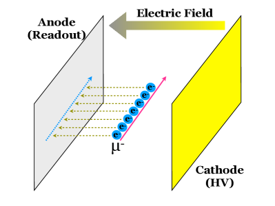
In this section, we describe the central working principle of a LArTPC detector in order to provide background as to what the images from LArTPCs capture. A LArTPC consists of a liquid argon volume sandwiched between anode and cathode planes. A large negative voltage is applied at the cathode plane in order to create a uniform electric field inside the rectangular volume. See Figure 1 for a drawing of the setup. When a charged particle traverses inside the volume (a muon in Figure 1), ionization electrons are created along its trajectory. The electric field pushes the electrons toward the anode plane at a constant velocity. Critically, the anode needs to be constructed with some method to read out the amount and location of ionization electrons which have drifted to it. Detailed summaries of existing LArTPC detectors cane be found in the references Acciarri et al. (2017b); Amerio et al. (2004).

Figure 1: A pictorial description of how a particle trajectory is recorded in a LArTPC, which consists of liquid argon volume sandwiched by cathode (right, yellow) and anode (left, gray) planes. When a muon traverses the argon volume, ionization electrons are created along the trajectory and subsequently drift toward the anode plane due to the electric field. The anode plane contains many electrodes for sensing the position and amount of the drifted charge. Their signals are amplified, digitized and recorded for later imaging.

II.1 Wire-based Detector

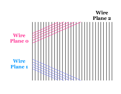
There are two major methods for constructing a LArTPC anode plane: “wire-based” and “pixel-based” readouts. The anode for a wire-based LArTPC consists of multiple planes where each plane, called a wire plane, is made out of many parallel wires. Among the multiple wire planes, the last – as seen from the drift electrons – is biased with the most positive electric potential and is called the collection plane, because the drift paths of the ionization electrons terminate on the collection wires and cause unipolar signals. The other wire planes, which are placed in front of the collection plane, are called induction planes. Wires on each induction plane are kept at a constant voltage such that ionization electrons will pass between wires toward the collection plane. Ionization electrons, as they pass the wires, induce a bipolar current signal on the wire which is the signal to be detected. From each wire plane, the digitized waveforms from the wires are combined in order to form a 2D image of particle trajectories. The time of arrival of the charge signal gives the location of the charge deposition along the drift axis because of the approximately constant drift velocity of the ionization electrons. Wires are separated by a constant pitch distance, typically a few mm. Each wire plane has a distinct wire orientation angle (Figure 2) which makes each 2D image a unique projection angle. The projection plane is the one perpendicular to the axis of the individual wires - for example, vertical wires project the 3D volume onto a plane in the horizontal axis.

The 3D shape of particle trajectories can be obtained only after combining information from multiple wire planes in the data analysis stage. Most existing and planned LArTPC detectors in neutrino oscillation experiments employ this “wire-based” design, including MicroBoone, ICARUS, SBND, and the DUNE far detectors Amerio et al. (2004); Acciarri et al. (2017b); Antonello et al. (2015); Acciarri et al. (2016). This design’s wide-spread use comes from the reduced number of readout electronics per detector volume. The use of wires to record projected positions means that the number of readout channels scales roughly with the length the anode plane as opposed to its area.

Figure 2: An illustration of an anode for a wire-based LArTPC. In this example, the wire-based anode consists of three wire planes and only a small portion of all wires are drawn for induction planes 0 and 1.

II.2 Pixel-based Detector

The anode plane of a pixel-based LArTPC consists of a 2D array of pixel electrodes, with each channel connected to its own charge-sensitive readout electronics. Example detectors of this class includes ArgonCube and the DUNE near detector Asaadi et al. (2018). The size of pixels is typically a few mm. Optimal combination of pixel size and shape is currently being investigated by R&D programs Dwyer et al. (2018). The pixelated anode records digitized waveforms of collected ionization electrons at each pixel pad. The location of each pixel provides 2D position of drift electrons when projected on the anode plane. Given the constant velocity of drift electrons, the digitization timing can be converted into a position of drift electrons along the drift direction. In combination, a pixel-based LArTPC allows imaging of 3D particle trajectories from raw waveform without the need of 3D point reconstruction - unlike wire-based LArTPCs. This relative ease of 3D position reconstruction is one of the pixel-based readout’s advantages, however the number of readout channels required scales with the area, not length, of the anode plane.

II.3 Physics Simulation for LArTPCs

Physics simulations of LArTPC experiments can be divided into three steps:

1. event generation, which creates a list of particles to be simulated in a detector,

2. tracking of particles, including decay and interactions with other particles and detector medium,

3. and simulation of the electronics signals from the result of particle tracking.

For most LArTPC experiments, the simulation routines are implemented within LArSoft Snider and Petrillo (2017), a community-driven software framework for simulation and data analysis. While LArSoft is open-source and many of the components are shared across experiments, each experiment must still specify many details such as detector materials, readout configurations, and more in order to build their respective simulation. Consequently, the experiment-specific implementations of LArSoft are not typically open-source. The experiment-specific components manifest primarily in step 1 and 3 in the list above, because each experiment has a different physics signal to look at as well as different detector configurations. On the other hand, step 2 above is almost identical among experiments except for the fact that the geometry of liquid argon volume may be different. This step uses Geant4 Agostinelli et al. (2003), a software developed over many decades in the field of High Energy Physics for tracking particle interactions in the detector medium (i.e. liquid argon).

In this paper, we present a data sample generated using our custom event generator (step 1) followed by a Geant4 particle tracking simulation run within LArSoft (step 2). This release of sample does not incorporate step 3 for which we need a dedicated effort to develop open-source algorithms for a hypothetical detector response. Instead, we applied spatial smearing of charge to every voxel in order to mimic a real detector resolution. This will be described in the following sections. While it lacks accurate detector-specific effects on signal, the generated images capture the geometrical and basic calorimetric features of particle trajectories in a LArTPC detector. The sample can be used for experiment-agnostic algorithm development including ML applications for reconstruction and analysis of LArTPC data.

III 2D/3D LArTPC Simulation Samples

Figure 3: Recorded energy deposition at the end of particle tracking simulation, visualized using the LArCV native data visualization tool. Left: energy deposition recorded per cubical cells. The color scale changes from dark blue, cyan, yellow, and red for increasing amount of energy per cell. Right: cells categorized into 5 colors based on the most dominating particle type in terms of deposited energy per cell. Five categories are protons (dark blue), Michel electrons (orange), delta rays (yellow), electromagnetic showers (green), and other particles (cyan) typically minimum ionizing particles such as muons and pions.

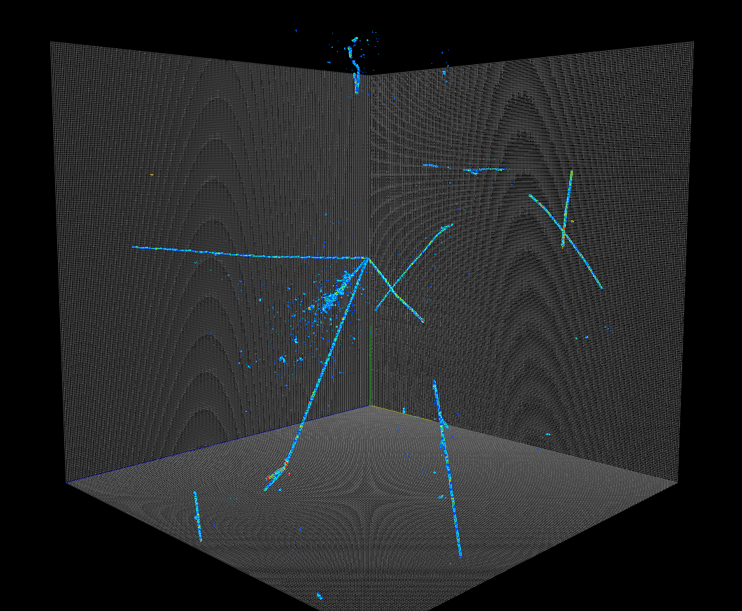
Our dataset is a simulation of particles created for the development of data analysis techniques for LArTPC detectors, and contains a total of 300,000 physics events generated using custom event generators  followed by a particle tracking simulation using Geant4. The samples are all independently simulated events, and consist of three different cubical volumes including $192^{3}$, $512^{3}$, and $768^{3}$ pixels, 100,000 samples each. In each event, two event generators, referred to as MultiPartVertex (MPV) and MultiPartRain (MPR), are used to generate a list of particles for tracking simulation. In this section, we describe the simulation process, recorded information, and data access methods.

III.1 Event Generator Simulation

In each event, the MPV generator simulates N particles all originating from a unique 3D point, called the vertex, where N is randomly set to an integer value between 1 and 6 with equal probability. There are five categories of particles that can be generated: electron, photon, (anti-)muon, charged (anti-)pion, and proton. Each category has two simulation parameters for generation: the range of kinetic energy and the maximum number of multiplicity per category as shown in Table 1. N particles are randomly drawn from available categories where multiplicity limit is not reached. The kinetic energy of a particle is determined within the specified range, and is distributed uniformly. Among the five categories, muon and pion can be either a particle or an anti-particle with equal probability. The reason for including both types is because the behaviors are different: stopped anti-muons decay 100% of the time with a positron emmission while stopped muons get captured by an argon nucleus more than half the time in LArTPCs. Thus including both types is possibly of interest for data reconstruction algorithm development. Neither existing nor future LArTPCs plan to observe anti-protons.

Category	Max. Multiplicity	Kinetic Energy [MeV]
Electron	1	50 to 1000
Photon	3	50 to 1000
(Anti-)Muon	1	50 to 1000
(Anti-)Pion	2	50 to 1000
Proton	2	50 to 400

Table 1: MPV generator configuration parameters including the maximum particle multiplicity limit per category and the range of kinetic energy allowed. Within this range the kinetic energy value is randomly assigned.

Category	Max. Multiplicity	Kinetic Energy [MeV]
Electron	5	50 to 1000
(Anti-)Muon	5	50 to 1000
Proton	5	50 to 400

Table 2: MPR generator configuration parameters including the maximum particle multiplicity limit per category and the range of kinetic energy allowed. Within this range the kinetic energy value is randomly assigned.

The MPR generator is similar to MPV except generated particles are not required to come out of the same vertex. The total number of particles generated by MPR is fixed to 10 in every event, and the start point is uniformly distributed in the simulated volume of liquid argon. Table 2 describes the list of categories and their configurations for MPR generator used for the public sample. The categories include electron, (anti-)muon, and proton. For MPR, the probability of each category to be chosen for a particle generation is not uniform across categories. It is set to 20%, 60%, and 20% for electron, (anti-)muon, and proton respectively. There is a weak motivation to populate the space with (anti-)muons which might make the simulated sample look closer to surface LArTPC detectors that are exposed to cosmic ray particles.

III.2 Particle Tracking Simulation

Following the generation of particles, tracking simulation is done using Geant4, version v4.10.1.p03 with physics list QGSP_BIC. within LArSoft. Geant4 propagates all particles and simulates both energy depositions in the medium as well as secondary interactions induced by the generated particles. In this simulation stage, the liquid argon volume is voxelized into many cubes of the same size with 3 mm side. Ionization energy deposition by charged particles traversing cells of the voxelized volume is recorded as a sparse matrix data for individual particles. This allows us to track energy depositions per cell per particle. In addition to energy deposition information, we also record summary information per particle that is generated by either an event generator or through secondary particle interactions during the tracking stage.

The recorded volume of the tracking simulation may be one of three different sizes: $192^{3}$, $512^{3}$, and $768^{3}$ pixels. In each case, the spatial resolution of each voxel is 3 mm. The location of the recorded cubic volume is determined under two conditions. First, it must contain the vertex defined by MPV event generator. Second, it must maximize the energy depositions of particles generated by MPV. Under these conditions, the position of the volume is set randomly. By construction, therefore, the MPV vertex can be found in an each event.

III.3 Spatial Smearing of Energy Deposition

The output of the particle tracking simulation is a collection of summary information per particle, and energy depositions per particle per cell of a voxelized volume. We refer to those outputs particle and particle-cluster information. For each pixel, smearing of the energy deposition is applied using a normal distribution with a spread of a unit voxel (3 mm). This makes a particle trajectory thicker as energy from a pixel is spread to its neighbor pixels. For every pixel, the value is computed again by summing contributing energy from neighbor pixels as a result of smearing. The sum of all pixel values remains the same before and after the smearing process.

III.4 Image of Particle Trajectories

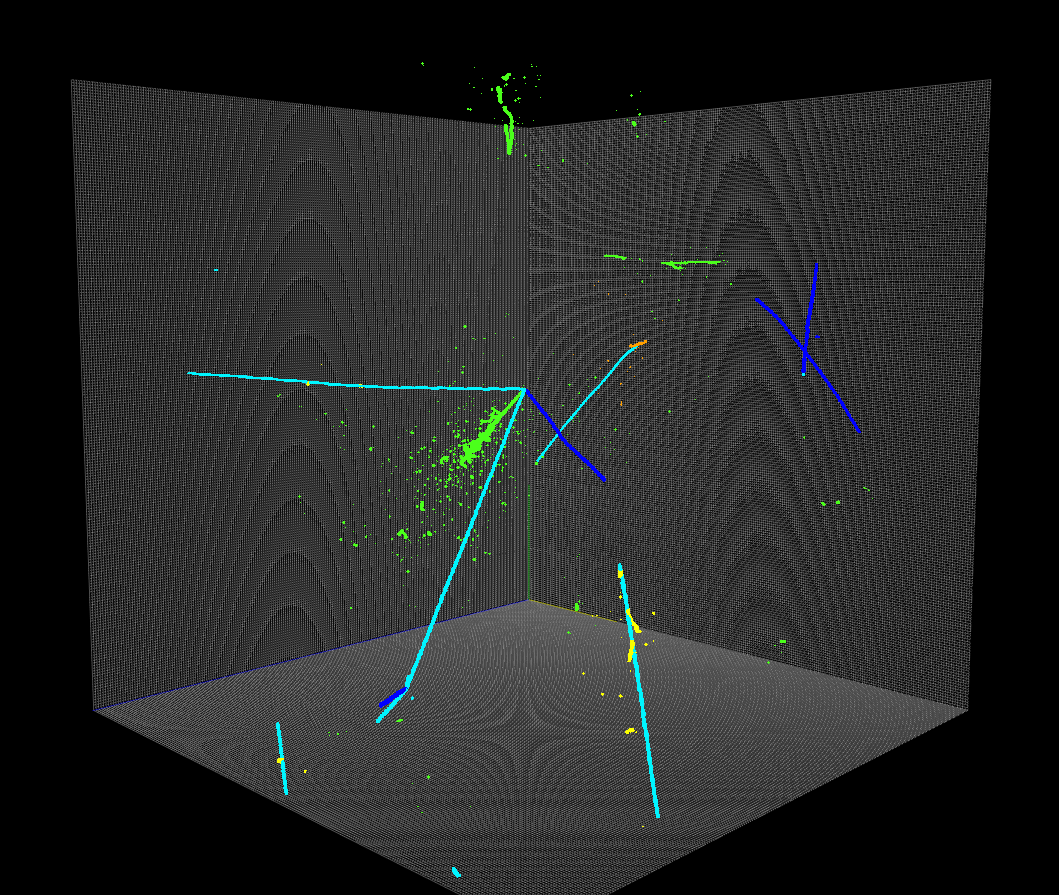
From the smeared energy depositions, we generate 3D energy deposition information, referred to as energy-3D information, in the detector by summing energy depositions per cell across all contributing particles. This is shown in the left of Figure 3, and resembles what a pixel LArTPC can detect in an ideal world where detector responses including readout electronics, electric field response, and recombination of ionization electrons are absent. While diffusion of ionization electrons in drift is not simulated, an artificial smearing of deposited energy is applied. Despite the lack of those simulation stages, topological and geometrical features in 3D images that pose challenges to LArTPC data reconstruction are still present.

In addition to energy-3D, segment-3D, which holds a category of particle types per pixel, is also created from particle information.

The segment-3D image is only different from the energy-3D by individual pixel values. The pixel values vary between 0 to 4 in integer steps and defined as follows.

1. Protons (a heavily ionizing particle), which have a “track” topology (1D line-shaped trajectory).

2. Other particles (typically minimum ionizing particles) with a “track” topology: (anti-)muon and charged (anti-)pion.

3. Electromagnetic (EM) particles (i.e. electrons, positrons and photons) which have a “shower” topology (containing many “Y”-shaped branches) .

4. Michel electrons, a decay electron and positron from a muon and anti-muon respectively.

5. Delta rays, knock-off electrons from track particles traversing the LAr volume.

The segment-3D information can be used to train an algorithm for pixel-level categorization, a task referred to as semantic segmentation in the field of CV, and is crucially useful for LArTPC data analysis Adams et al. (2018).

Finally, the 2D projections of energy-3D and segment-3D are created, referred to as energy-2D and segment-2D in this paper. Those projections are simple 2D projections along the principle 3D coordinate axis including x-y, y-z, and z-x plane projections. The contents of the output files can be used to train ML algorithms for all of tasks in the list of bullets above.

III.5 Simulation Output

Figure 4: LArTPC image data is generally sparse although locally dense. The top figure shows the number of total pixel count per 3D image. The blue, orange, and green colors of histograms correspond to $192^{3}$, $512^{2}$, and $768^{3}$ image size. The bottom figure shows the fraction of non-zero pixels in the cubic volume.

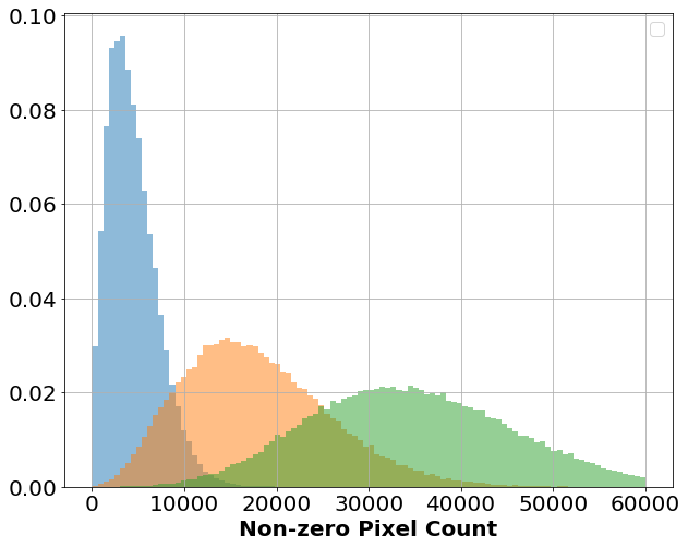
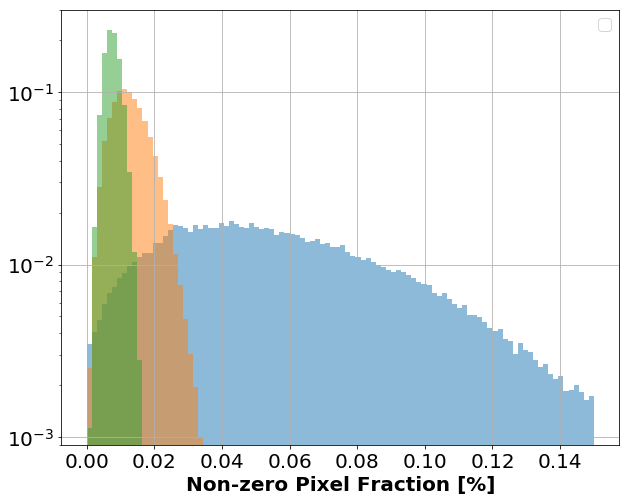
Sparse 2D and 3D matrix data representations in the LArCV software framework are used for efficient storage of all matrix data which includes particle-cluster, energy-3D, segment-label-3D, energy-2D, and segment-label-2D. LArTPC image data is generally sparse, but locally dense (i.e. no gap in a recorded particle trajectory). Figure 4 shows that, for energy-3D, the fraction of non-zero pixels in three simulated volume sizes are well below 1 %. Moreover, because in most cases a particle trajectory is locally a one-dimensional line, the increase in the number of non-zero pixels does not scale in the same manner as the total number pixels required for a volume to contain a longer trajectory. Therefore a zero-suppressed matrix data representation is crucial to keep a reasonable storage data file size.

III.6 Data Challenges

Physics Task	Input Data	Label	Computer Vision Task
Particle ID	particle-cluster	particle	Image-level classification (multinomial logistic regression)
Particle Kinematics	particle-cluster	particle	Image-level regression
(energy, direction)	or energy-2D/3D
Particle Trajectory	energy-2D/3D	particle-cluster	Object instance segmentation (pixel clustering)
Reconstruction
Position/Vertex	energy-2D/3D	particle	Object detection / position regression
Reconstruction
3D Point	energy-2D	energy-3D	2D to 3D image reconstruction (inverse process)
Reconstruction

Table 3: Physics tasks with input data and corresponding tasks for CV techniques development. The label column shows the label information that can be used for supervised training method.

The challenge of topological LArTPC data reconstruction is to start from energy-2D or energy-3D information and derive higher level information including:

• a pixel-level particle category information (i.e. segment-3D data),

• a cluster of pixels corresponding to individual particle trajectory (i.e. particle-cluster data),

• particle-level information including a particle type, momentum, start/end points and directions (i.e. particle data),

• image-level information including total energy, the interaction vertex, and hierarchical correlation (i.e. “flow”) of particles that can be retrieved from particle data.

These tasks follow the order of a typical data analysis workflow for LArTPC images, and each has an analog to an image analysis task in CV. Our dataset provides necessary information (i.e. “labels”) for supervised training of ML algorithms. Table 3 summarizes a set of challenges associated with this dataset, necessary label information from the dataset for supervised learning, and corresponding tasks in CV.

III.7 Hosting and Organization of Data

Our dataset is hosted currently by the Open Science Framework (OSF) under CC-by-Attribution 4.0 international license. The OSF is one of several free data hosting tiers that can be directly cited for publications in major journals. It also includes features to generate the digital object identifier (DOI) per data set. In addition, it provides a rich set of web browser and command-line interfaces for simple upload and download of data files.

Sub-folder Name	Contents
cluster	particle-cluster
data	energy-3D, segment-3D
data-2d	energy-2D, segment-2D
particle	particle

Table 4: Sub-folder name under 192px, 512px, and 768px top folders of the dataset and the contents in files.

The OSF data storage is organized in a hierarchical manner. The top level storage of the dataset contains three folders named as 192px, 512px, and 768px which contain datasets with corresponding volume size following the folder name. There are four sub-folders under each of them: cluster, data, data-2d, and particle. These sub-folders hold data files where the contents of each data file are summarized in Table 4. Under each sub-folder, there exist same number of data files with a common file suffix “XX.root” where XX is a zero-filled two digit integers to match the contents of files across sub-folders. There are 10 files under each sub-folder of 192px and 512px, and each file contains 10,000 events, which makes 100,000 events from 10 files for those two volume sizes. Under the sub-folders of 768px, there are 20 files where each file contains 5,000 events. The reason for splitting into more files for this volume size is the maximum single file size limitation imposed by OSF, which is 5 GB/file.

IV Interacting with the Dataset

Accessing the contents of the dataset can be done using LArCV, which is primarily written in C++ with an extensive Python API. LArCV is maintained by the Deep Learn Physics (DLP) organization and software containers are distributed for algorithm development and data analysis use. The currently supported container types are Docker Merkel (2014) and Singularity Sochat VV (2017). A dedicated data interface API is also prepared for this open data set, and is described in this section.

IV.1 Software Containers

Container images can be found in the DLP repositories hosted by docker-hub and singularity-hub. The recipe files used to build these containers can be found in DLP software repositories larcv2-docker and larcv2-singularity respectively. Built image tags and versions are closely mirrored between images among those two container types.

IV.2 Data Interface APIs

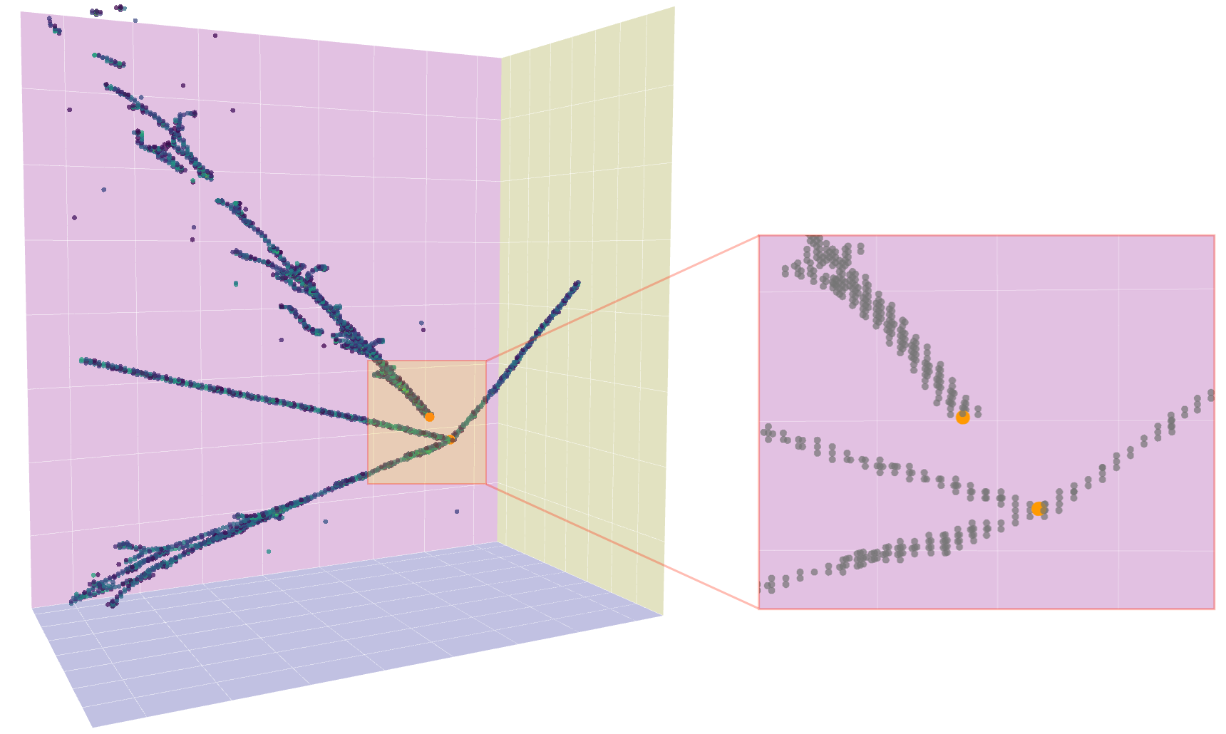
There are two recommended ways to open and interpret data files under the software container environment. A straightforward option is to use Python API functions from the dlp_opendata_api repository. The example script included in the repository demonstrates how one can open a file, move a data pointer among different samples, and retrieve data in numpy array data format, which is one of the most popular representations with connections to ML libraries. The example also shows how to match 3D imaging data with particle meta information, such as start and end points of a trajectory using plotly data visualization tool. Figure 5 shows an example visualization of a sample using plotly and numpy array of particle energy depositions and start positions obtained using the APIs. A similar visualization example is included in the prepared demo script.

Figure 5: Visualization of a particle trajectories (energy depositions) from a dataset sample using prepared Python APIs. The orange sphere indicates the start points of particles, which can be used for supervised training of ML algorithms to regress the three-dimensional start position of particles.

Separately, LArCV provides methods to interface to data using both Python and C++. While there is more overhead cost in learning the LArCV framework, this method provides multi-threaded routines for reading data from files and loading to computer memory. This scheme supports configurable options to load data in either dense or sparse matrix format. While these routines are written in C++, APIs are provided also in Python. Fast data loading using native APIs in the LArCV framework may be useful for training ML algorithms and running fast inference on a large set of data samples. A python interface is also provided to serve as a distributed IO interface for MPI based applications such as distributed learning. Examples on how to use LArCV file reader APIs for training deep neural networks is described in a tutorials and wiki.

V Conclusion

We have presented PILArNet and the first open LArTPC dataset of simulated particle trajectories as an initial contribution. The first set presented in this paper contains 300,000 sample statistics with various labels that can be used for supervised ML algorithm training. The dataset is produced using Geant4 and LArSoft, common public software frameworks in the community of LArTPC experiments, and stored in LArCV files with a sparse matrix data representation which serves well for sparse particle energy depositions in LArTPC detectors. The dataset is hosted within the Open Science Framework, which is a recognized scientific data sharing tier highly integrated with industrial cloud services. The software containers are the modern approach to establish an identical software execution and development environment, and therefore they improve reproducibility of research. Our Docker and Singularity software container images are made available to ease the preparation of a data analysis environment.

Recent advancements in ML have a potential to address many challenges in science research. The open datasets have been the core of evolution in the field of ML, and are most effective ways to form a connection between domain experts and researchers from outside fields. PILArNet follows this model, and it is aimed to seed cross-experimental, cross-disciplinary collaborations in order to address challenges in analyzing data of LArTPC and other particle imaging detectors. PILArNet will continue to evolve in both variety and maturity to aid domain-specific ML technique adaptations and to enable physics discoveries.

VI Acknowledgement

This work is supported by the U.S. Department of Energy, Office of Science, Office of High Energy Physics, and Early Career Research Program under Contract DE-AC02-76SF00515. This research used resources of the Argonne Leadership Computing Facility, which is a DOE Office of Science User Facility supported under Contract DE-AC02-06CH11357.

References

- Krizhevsky et al. (2017) A. Krizhevsky, I. Sutskever, and G. E. Hinton, Commun. ACM 60, 84 (2017).
- LeCun et al. (2015) Y. LeCun, Y. Bengio, and G. Hinton, Nature 521, 436 (2015).
- LeCun and Cortes (2010) Y. LeCun and C. Cortes, (2010).
- (4) A. Krizhevsky, V. Nair, and G. Hinton, .
- Deng et al. (2009) J. Deng, W. Dong, R. Socher, L. jia Li, K. Li, and L. Fei-fei, In CVPR, (2009).
- Lin et al. (2014) T. Lin, M. Maire, S. J. Belongie, L. D. Bourdev, R. B. Girshick, J. Hays, P. Perona, D. Ramanan, P. Dollár, and C. L. Zitnick, CoRR abs/1405.0312 (2014), arXiv:1405.0312 .
- Everingham et al. (2010) M. Everingham, L. V. Gool, C. K. I. Williams, J. Winn, and A. Zisserman, “The pascal visual object classes (voc) challenge,” (2010).
- Chang et al. (2015) A. X. Chang, T. A. Funkhouser, L. J. Guibas, P. Hanrahan, Q. Huang, Z. Li, S. Savarese, M. Savva, S. Song, H. Su, J. Xiao, L. Yi, and F. Yu, CoRR abs/1512.03012 (2015), arXiv:1512.03012 .
- Simonyan and Zisserman (2014) K. Simonyan and A. Zisserman, “Very deep convolutional networks for large-scale image recognition,” (2014), arXiv:1409.1556 [cs.CV] .
- Szegedy et al. (2014) C. Szegedy, W. Liu, Y. Jia, P. Sermanet, S. Reed, D. Anguelov, D. Erhan, V. Vanhoucke, and A. Rabinovich, “Going deeper with convolutions,” (2014), arXiv:1409.4842 [cs.CV] .
- He et al. (2015) K. He, X. Zhang, S. Ren, and J. Sun, “Deep residual learning for image recognition,” (2015), arXiv:1512.03385 [cs.CV] .
- Huang et al. (2016) G. Huang, Z. Liu, L. van der Maaten, and K. Q. Weinberger, “Densely connected convolutional networks,” (2016), arXiv:1608.06993 [cs.CV] .
- Xie et al. (2016) S. Xie, R. Girshick, P. Dollár, Z. Tu, and K. He, “Aggregated residual transformations for deep neural networks,” (2016), arXiv:1611.05431 [cs.CV] .
- Chen et al. (2017) W. Chen, Muyuan Cand Dai, S. Sun, D. Jonasch, C. He, M. Schmid, W. Chiu, and S. Ludtke, Nat Methods 14, 983 (2017).
- Ferreira (2018) D. R. Ferreira, (2018), arXiv:1811.00333 .
- Acciarri et al. (2017a) R. Acciarri et al. (MicroBooNE), Journal of instrumentation 12, P03011 (2017a).
- Adams et al. (2018) C. Adams et al. (MicroBooNE), (2018), arXiv:1808.07269 [physics.ins-det] .
- Amerio et al. (2004) S. Amerio et al. (ICARUS), Nuclear Instruments and Methods in Physics Research Section A: Accelerators, Spectrometers, Detectors and Associated Equipment 527, 329 (2004).
- Acciarri et al. (2017b) R. Acciarri et al. (MicroBooNE), Journal of Instrumentation 12, P02017 (2017b).
- Antonello et al. (2015) M. Antonello et al. (MicroBooNE, LAr1-ND, ICARUS-WA104), (2015), arXiv:1503.01520 [physics.ins-det] .
- Acciarri et al. (2016) R. Acciarri et al. (DUNE), (2016), arXiv:1601.02984 [physics.ins-det] .
- Radovic et al. (2018) A. Radovic, M. Williams, D. Rousseau, M. Kagan, D. Bonacorsi, A. Himmel, A. Aurisano, K. Terao, and T. Wongjirad, Nature 560, 41 (2018).
- Dominé and Terao (2019) L. Dominé and K. Terao, “Scalable deep convolutional neural networks for sparse, locally dense liquid argon time projection chamber data,” (2019), arXiv:1903.05663 [cs.CV] .
- Ju et al. (2020) X. Ju, S. Farrell, P. Calafiura, D. Murnane, Prabhat, L. Gray, T. Klijnsma, K. Pedro, G. Cerati, J. Kowalkowski, G. Perdue, P. Spentzouris, N. Tran, J.-R. Vlimant, A. Zlokapa, J. Pata, M. Spiropulu, S. An, A. Aurisano, J. Hewes, A. Tsaris, K. Terao, and T. Usher, “Graph neural networks for particle reconstruction in high energy physics detectors,” (2020), arXiv:2003.11603 [physics.ins-det] .
- Agostinelli et al. (2003) S. Agostinelli et al. (GEANT4), Nucl. Instrum. Meth. A506, 250 (2003).
- Snider and Petrillo (2017) E. L. Snider and G. Petrillo, Proceedings, 22nd International Conference on Computing in High Energy and Nuclear Physics (CHEP2016): San Francisco, CA, October 14-16, 2016, J. Phys. Conf. Ser. 898, 042057 (2017).
- Asaadi et al. (2018) J. Asaadi et al., (2018), arXiv:1801.08884 [physics.ins-det] .
- Dwyer et al. (2018) D. Dwyer, M. Garcia-Sciveres, D. Gnani, C. Grace, S. Kohn, M. Kramer, A. Krieger, C. Lin, K. Luk, P. Madigan, C. Marshall, H. Steiner, and T. Stezelberger, Journal of Instrumentation 13, P10007 (2018).
- Merkel (2014) D. Merkel, Linux J. 2014 (2014).
- Sochat VV (2017) K. G. Sochat VV, Prybol CJ, PLoS ONE 12 (2017).