Sensitivity and Dimensionality of Atomic Environment Representations
used for Machine Learning Interatomic Potentials

Abstract

Faithfully representing chemical environments is essential for describing materials and molecules with machine learning approaches. Here, we present a systematic classification of these representations and then investigate: (i) the sensitivity to perturbations and (ii) the effective dimensionality of a variety of atomic environment representations, and over a range of material datasets. Representations investigated include Atom Centred Symmetry Functions, Chebyshev Polynomial Symmetry Functions (CHSF), Smooth Overlap of Atomic Positions, Many-body Tensor Representation and Atomic Cluster Expansion. In area (i), we show that none of the atomic environment representations are linearly stable under tangential perturbations, and that for CHSF there are instabilities for particular choices of perturbation, which we show can be removed with a slight redefinition of the representation. In area (ii), we find that most representations can be compressed significantly without loss of precision, and further that selecting optimal subsets of a representation method improves the accuracy of regression models built for a given dataset.

I Introduction

Machine Learning (ML) as a predictive modelling tool has gained much attention in recent years in fields ranging from biologyBaldi and Brunak (2001), and chemistryNoordik (2004) to materials scienceHil (2016); Bartók et al. (2017), building on decades of successful applications in image recognition, natural language processing and artificial intelligence (AI) Huang et al. (2019); Zemmari and Benois-Pineau (2020) While machine learning has also been increasingly popular in many fields due to its relatively simplicity of application and powerful prediction features, a key driving force of is the increasing availability of information through data repositories, archives and databases of materials and molecule that include billions of structuresRuddigkeit et al. (2012); Hil (2016). In recent years, a large number of ML models for materials and molecules have been developed and many novel representation methods have been proposed Behler (2011); Bartók, Kondor, and Csányi (2013); Huo and Rupp (2017); Isayev et al. (2017); Schütt et al. (2018); Zhou et al. (2018); Ziletti et al. (2018); Novoselov et al. (2019). Representations are the feature sets used as input data for data-driven machine learning models, which, after training, can be used to predict quantities of interest.

Some of these databases are focused on molecular configurations such as PubChemKim et al. (2018), DrugBankWishart et al. (2017) and ChEMBLMendez et al. (2018) are widely used in biological, chemical, and pharmacological applications driven by high-throughput screening for drug design and novel molecule discovery. Other databases such as the Cambridge Structural Database (CSD)Groom et al. (2016) include crystals as well as small molecules. While these databases contain mostly molecular structures with their chemical or biological properties, recent efforts such as the Materials ProjectJain et al. (2013); materialsproject.org , Automatic FLOW for Material Discovery Library (AFLOWLIB.org)Curtarolo et al. (2012a, b), Open Quantum Materials Database (OQMD)Saal et al. (2013); Kirklin et al. (2015), and the NOMAD archivenomad coe.eu (2019) (which collates data from many other databases as well as contains data that are not available at them) now provide extensive electronic structure results for molecules, bulk materials, surfaces and nanostructures in a range of ordered and disordered phases, with chemical composition ranging from inorganic systems to metals, alloys, and semiconductors. With recent advancements in materials databases, access is available to billions of properties of materials and molecules and millions of high-accurate calculations through online archives. With such an extensive and diverse collection of molecular and materials data to hand, we can ask questions such as how to identify of the most informative subset of data for a particular class of materials, and how best to interpret it for prediction through ML models. These questions are relevant for both classification and regression applications: for example, classifying materials as metallic or semiconducting, or predicting the band-gap from structure, respectively. In both cases, the input data is constructed from information ranging from basic physical and chemical properties to precise geometrical information based on atomic structure and bonding topology. There have been many studies to determine these input information which are named as descriptors, fingerprints or representations Chen et al. (2018); Geiger and Dellago (2013); Collins et al. (2018); Muratov et al. (2020); Reveil and Clancy (2018); Zhou et al. (2018); Behler (2016)

Here, we define the prediction problem as,

$${\bf t}(\chi_{k})\simeq f(\{M_{a}(\{{\bf V}_{b}\})\})$$ (1)

where $\mathbf{t}$ is the target property of the material, $\chi_{k}$ represents the structure with index $k$ within the database, $M_{a}$ is the machine learning model with identifier $a$, and ${\bf V}_{b}$ is the input representation determined with identifier $b$ that is used for optimizing $f$. We define representations as

$${\bf V}_{b}(\chi_{k})=g(\{h_{i}(x_{j},\{\alpha_{1},\alpha_{2},...,\alpha_{m}\})\})$$ (2)

where, $x_{j}$ are the coordinates of atom with index $j$ within structure $k$, $\alpha_{m}$ is a physical or chemical property of the material and chemical environment, $h_{i}$ is the descriptor mapping from the input space to hyper-dimensional space with each dimension being an input feature of model $M$ and $g$ is the encoding function that combines all of the $h_{i}$ descriptors to make an overall representation. In Equation 1, the optimization of the parameters of $f$ can be performed either for a single model $M$ or for multiple models $M_{1},M_{2},\ldots$ in combination with potentially multiple different representations ${\bf V}_{b}$.

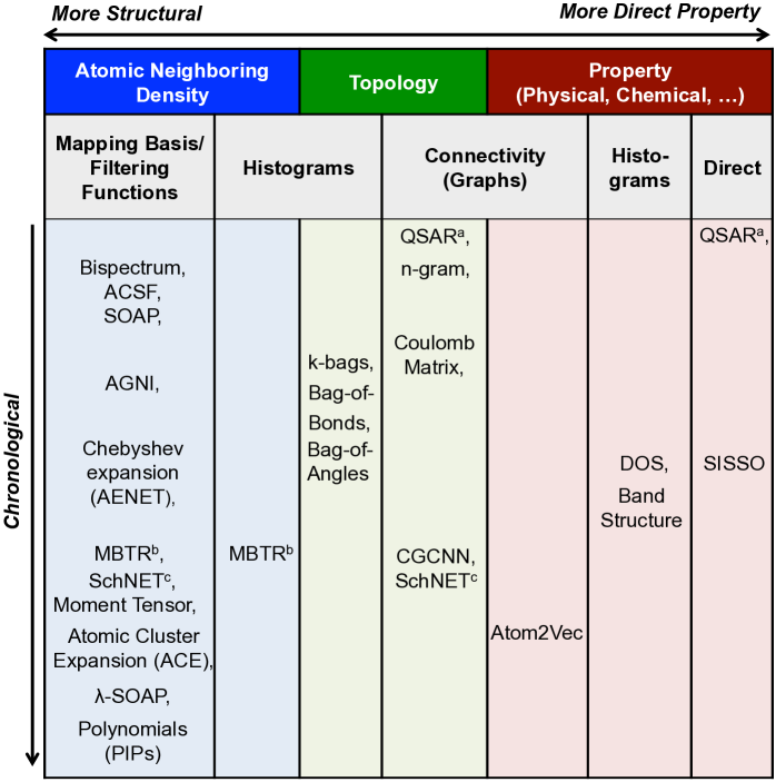
Figure 1: Classification of representations based on their method of construction (horizontal axis) and when they were first proposed (vertical axis). QSAR and SISSO do not indicate representations but instead indicates the representations that are constructed or selected using these methods (see text). ^a,b,c representations that are classified with multiple methods: Direct & Connectivity, Histogram & Mapping functions, and Connectivity & Mapping functions.

From this general perspective, many approaches can be combined to form a predictive model, raising the critical open question of how to optimally choose which pieces of information are needed to represent a material through descriptors and how to combine these to form representations. These can vary from defining sets of physical and chemical properties and atomic geometries to specialized hyper-dimensional mapping algorithms (see Figure 1). These representations and their building blocks, the descriptors can be classified into three broad classes based on their construction: (i) atomic neighborhood density definitions, (ii) topology expansions and (iii) property-based selections. The representations can be further grouped according to their combination rules, mapping basis or filtering functions, histograms, connectivity maps or graphs, and finally direct contributions from material properties. Within each category, there have been various developments of representations and many successful applications, which we review briefly in Section II below, before specialising on atomic neighbourhood densities in Section III. Section IV lists the data sources used here for evaluating representations, and Section V describes our analysis methodology. Results and discussion follow in Section VI.

II Representation Classes

II.1 Property-based representations

The idea of classification of molecules based on the relationships between their structure and the resulting activities or properties is an underpinning approach of modern chemistryRoy, Kar, and Das (2015). However, using theoretical descriptors to identify the relations was first utilised for quantitative structure-activity/property relationship (QSAR/QSPR) modellingLo et al. (2018); Roy, Kar, and Das (2015), starting with the work of Wiener and Platt in 1947, who used indices based on chemical graph theoryRoy, Kar, and Das (2015). We use the name QSAR refer to both QSAR/QSPR models.

QSAR models are highly successful predictive modelling approaches in chemistry and biology in various applications Lo et al. (2018); Roy, Kar, and Das (2015). These models are determined using sets of descriptors that are defined through a selection of physical, chemical properties of materials and/or structural descriptors of molecules such as atoms and their molecular bonds from chemical topology information to graphs where the fractions of the bonding information is simplified to indices.Roy, Kar, and Das (2015); Lo et al. (2018); Danishuddin and Khan (2016)

The success of QSAR mostly depends on the choice of descriptor sets, and in particular, determining the optimum number of descriptors in such sets Lo et al. (2018). For example, compressed-sensing approaches have been developed to systematic select the optimal set of the descriptors Shahlaei (2013); Danishuddin and Khan (2016).

Direct property-based approaches also employ reduction techniques to identify optimal models $\{M_{a}\}$ in Equation 1, by choosing mathematical operators for $g$ that combine descriptors from a given set of $\{h_{i}\}$ with $x_{j}$, $\{\alpha_{m}\}$ or both. This optimization scheme, referred to as sure independence screening and sparsifying operator (SISSO), has been successfully applied as a classification technique to group materials (e.g. metals vs. non-metals) and as a regression method to determine a target property of interest.Ouyang et al. (2018)

The connectivity information of each species in the chemical stoichiometry has also been introduced recently with atom2vecZhou et al. (2018) method as a representation where a single atom-to-environment connectivity matrix can be constructed. This simple approximation enables the approach to be used to screen billions of materials and make predictions such as identifying possible candidates for Li-ion battery elements Cubuk, Sendek, and Reed (2019) based only on chemical composition and stoichiometry.

Recent efforts also address the direct usage of electronic structure data to define descriptors. In these methods, the essence of the electronic structure information is extracted through histograms over density-of-states (DOS) Yeo et al. (2019) or over the selected band structures Oses, Toher, and Curtarolo (2018) into the descriptor vectors.

II.2 Topology-based representations

In this group of descriptors, topological information is derived from the full connectivity graph of the atomic environment instead of simplified indices. Examples of this class of methods include the Coulomb and Sine MatricesHimanen et al. (2019), n-gram graphsLiu, Demirel, and Liang ; Sutton et al. (2019), and Graph based Neural Network (NN) models such as DTNNSchütt et al. (2017), SchNETSchütt et al. (2018), CGCNNXie and Grossman (2018). While Coulomb and Sine matrices use atom-to-atom connection information directly and are thus based on the inferred chemical bonding between atoms, the input representations of Graph Neural Network models are defined through neighborhood analysis of atomic connectivity graphs and can be constructed from the full $n$-body topology.

Another approach to use topology information such as bonds, angles and higher-order many-body contributions is to group them into sets of building blocks and apply histograms on these blocks over the input datasets. Several successful implementations of these approach are Bag-of-Bonds (BoB)Hansen et al. (2015) and its analogy to higher order contributions for example, Bag-of-Angles and k-bags.

Topology information provides atomic connectivity data and is very useful for structural similarity comparison, since this information is automatically invariant under changes in the atomic positions. Topology is a blueprint of chemical bonding definitions for materials or molecules. However, it is not a physical observable and therefore it cannot be constructed uniquely. For novel material discovery one needs to use electronic structure calculations to generate new data comprising the properties and construction of structural representations of uncharted material compositions. However, such database construction for new structures is extremely expensive.

II.3 Atomic Neigbourhood Density representations

Modelling materials and molecules at the atomic scale is essential to identify novel materials for applications of interest or to determine candidate molecules with specific function in a desired medium. When accuracy and reliability of concern, preference is usually given to ab initio calculations. However, these first-principles calculations are inaccessible for systems requiring long time-scales and/or large numbers of atoms. To significantly reduce the computational cost, interatomic potentials or force fields are employed to define the interactions between atoms using parametrized forms of functions in place of the electronic interactions. Although these approaches allow larger numbers of atoms to be included in simulations and provide access to much longer time-scales, their prediction accuracies are typically limited as a result of simplified models describing interatomic interactions.

A prominent recent trend has been to address this limitation with machine learning interatomic potentials (MLIPs), i.e. by replacing fixed functional forms for the atomic interactions with data-driven machine learning models that map from atomic positions to potential energy surface, via descriptors based on the local neighbourhood of each atom. This approach based on atomic-densities extraction has been applied in pioneering models using symmetry functions Behler (2011) and more recently the so-called smooth-overlap of atomic positions (SOAP)Bartók et al. (2010); Bartók, Kondor, and Csányi (2013). Symmetry functions are widely used in neural network interatomic potentials (NNP)Behler (2011, 2016); Artrith, Morawietz, and Behler (2011); Artrith and Urban (2016) successfully for many molecules and materials including water, crystals with various phasesCubuk et al. (2017), amorphous solids in various concentrationsSosso et al. (2012); Onat et al. (2018), while SOAP is typically incorporated in Gaussian Approximation Potentials (GAP)Bartók et al. (2010); Bartók, Kondor, and Csányi (2013). GAP has been applied to many molecules and materials.Dragoni et al. (2018); Deringer, Caro, and Csányi (2019); Bernstein et al. (2019); Bartók et al. (2017)

In this final class of descriptors, there have been many developments in recent years. In addition to atom-centered symmetry functions (ACSF) and SOAP descriptors, different basis expansions such as Bispectrum and Chebyshev polynomials have also been utilized in SNAP potentialsThompson et al. (2015); Wood and Thompson (2018) and NNPsArtrith, Urban, and Ceder (2017), respectively. Further advances are also provided in ML models based on atomic and many-body expansions with tensor representations such as Many-Body Tensor Representation (MBTR)Huo and Rupp (2017).

An alternative approach is to employ linear regression using a symmetric polynomial basis. This approach was pioneered by Bowman and Braams Braams and Bowman (2009), while more recent symmetric bases are the Moment Tensor potentials (MTP) Novoselov et al. (2019) and the Atomic Cluster Expansion (ACE) Drautz (2019). The MTP and ACE basis are also based on density projections and therefore closely related to the descriptors described above. In particular, ACE can also be seen as a direct generalisation of SOAP and SNAP providing features of arbitrary correlation order.

Recent works have demonstrated that the atomic-density representations can be unified in a common mathematical frameworkWillatt, Musil, and Ceriotti (2019), and that the descriptors can be decorated with additional properties to extend their capabilities, such as in $\lambda$-SOAP representations for learning from tensor propertiesWillatt, Musil, and Ceriotti (2019).

For all these ML models, different combinations of descriptors and representations have been used in many studies and for a wide range of materials. Deringer et al. (2018); Bernstein et al. (2019); Zuo et al. (2020) As these descriptors and representations are general structural identifiers, they can also be utilized within different regression models other than the ML models for which they were primarily developed. A recent work also shows the comparison of different regressors with these representations.Sutton et al. (2019) While different approaches have been utilized in these studies, comparative assessments of the representation approaches have thus far been limited. Studies for the property and topology based descriptors on the QSAR feature sets and the performance of graph based NN models show that selection of optimal descriptor sets are very important to ensure high predictive accuracy of the ML modelsZuo et al. (2020). A number of studies of the atomic neighborhood density approaches provide analyses primarily based on trained models’ precision on available datasets Zuo et al. (2020) but so far there is no performance assessment on descriptors and representations for materials and molecules focused solely structure to hyper-dimensional encoding.

Following the works by HuoHuo and Rupp (2017) and JägerJäger et al. (2018), we identify the essential properties of descriptors and representations for encoding materials and molecules as follows:

1. Invariance: descriptors should be invariant under symmetry operations: permutation of atoms and translation and rotation of structure.

2. Sensitivity (local stability): small changes in the atomic positions should result in proportional changes in the descriptor, and vice versa.

3. Global Uniqueness/Faithfulness: the mapping of the descriptor should be unique for a given input atomic environment (i.e. the mapping is injective).

4. Dimensionality: relatedly, the dimension of the spanned hyper-dimensional space of the descriptor should be sufficient to ensure uniqueness, but not larger.

5. Differentiability: having continuous functions that are differentiable.

6. Interpretability: features of the encoding can be mapped directly to structural or material properties for easy interpretation of results.

7. Scalability: ideally, descriptors should be easily generalized to any system or structure with a preference to have no limitations on number of elements, atoms, or properties.

8. Complexity: to have a low computational cost so the method can be fast enough to scale to the required size of the simulations and to be used in high-throughput screening of big-data.

9. Discrete Mapping: always map to the same hyper-dimensional space with constant size feature sets, regardless of the input atomic environment.

In this article, we concentrate our efforts on analysing sensitivity (i.e. local stability) and compressibility (i.e. dimensionality) of the selected set of descriptors and representations, and do not address uniqueness/faithfullness; for an interesting recent investigation of this important issue see Ref. Pozdnyakov et al., 2020. Scalability, Complexity, and Discrete Mapping are also not addressed here as these are mainly related to the implementation and cost of methods in ML models such as the evaluation costs of MLIPs or scalability limits of ML models, which are outside the scope of this work. On the other hand, the hunt for the interpretability of ML models considering the construction of the descriptors is not a new concept and has been studied in the context of QSAR modelsMik (2019) and many-body descriptorsPronobis, Tkatchenko, and Müller (2018). As also discussed in property-based representations, interpretability is automatically inherited by models that are built directly from properties. As the concept depends on the application of the ML models, we leave addressing this for future studies. While there have been many related efforts on the analysis of property and topology based descriptors Shahlaei (2013); Danishuddin and Khan (2016); Ouyang et al. (2018), we choose to focus here on the atomic neighborhood density based descriptors along with representative descriptors from three groups of mapping basis functions, tensor representations, and polynomial representations as follows: ACSF, Chebyshev polynomials in SF (CHSF), SOAP, SOAPlite, MBTR, and ACEDrautz (2019). We provide an analysis of the sensitivity and local stability of the descriptors as well testing their invariance under symmetry operations. We further assess the descriptors information packing ability using CUR matrix decomposition, farthest point search (FPS) and principal component analysis (PCA) dimension reduction techniques. We also provide analyses using linear and kernel ridge regression methods on the selected features from CUR to showcase the effect of the dimensionality of representations on ML models.

III Atomic Neighborhood Density Representations

The descriptors sharing neighborhood density extraction can be unified in a general atomic expansion following the works in Ref. Drautz, 2019 and Willatt, Musil, and Ceriotti, 2019 and can be defined by,

$$V_{b}=\{b_{i,n},b_{i+1,n},...\},i=1,..,N$$ (3)

where

$$b_{i,n}=\sum_{j}R_{n}(x_{i},x_{j}).$$ (4)

Here, $x_{i}$ is the position of atom $i$ and $b_{i,n}$ can be expressed with radial and angular basis functions or as a polynomial expansion. In the following, we will give a brief summary of selected atomic neighborhood density representations based on the above definition. These are Atom Centered Symmetry Functions (ACSF), Chebyshev polynomial representations, Smooth Overlap of Atomic Positions (SOAP), Many-Body Tensor Representation (MBTR), and Atomic Cluster Expansion (ACE).

III.1 Atom Centered Symmetry Functions (ACSF)

The descriptors of atom centered symmetry functions were introduced by Behler and Parrinello with their atomic neural network potentials (NNP) Behler (2011); Artrith, Hiller, and Behler (2013) and further used in a wide variety of applications Behler (2011); Artrith, Hiller, and Behler (2013); Artrith, Morawietz, and Behler (2011); Cubuk et al. (2017); Onat et al. (2018); Jäger et al. (2018). The method extracts atomic environment information for each atom in the configuration using radial contributions given by

$$b^{r}_{i}=\sum_{j\neq i}^{N_{j}}g^{r}(R_{ij})$$ (5)

and angular contributions of the form

$$b^{a}_{i}=\sum_{j\neq i}^{N_{j}}\sum_{k\neq j\neq i}^{N_{k}}g^{a}(A_{ijk})$$ (6)

where the distances $R_{ij}=|\mathbf{R}_{j}-\mathbf{R}_{i}|$ and angle dependent contributions are defined through their cosines via $A_{ijk}=\cos\theta_{ijk}$ and $\cos\theta_{ijk}=\mathbf{R}_{ij}\cdot\mathbf{R}_{jk}/(|\mathbf{R}_{ij}||\mathbf{R}_{ik}|)$ and are invariant under symmetry operations of translations and rotations, hence the name symmetry functions. While many symmetry functions have been proposed Behler (2011), two choices of functions commonly used for $b^{r}$ and $b^{a}$ in many applicationsBehler (2011); Artrith and Kolpak (2014); Artrith and Urban (2016); Artrith, Urban, and Ceder (2017); Onat et al. (2018); Imbalzano et al. (2018) take the radial function to be centered on atom $i$ to be defined as

$$b^{r}_{i}=G^{2}_{i}=\sum_{j\neq i}e^{-\eta(R_{ij}-R_{s})^{2}}\cdot f_{c}(R_{ij})$$ (7)

and the angular function centred on atom $i$ as

$$\begin{split}b^{a}_{i}=G^{4}_{i}=&2^{1-\zeta}\sum_{j\neq i}\sum_{k\neq i,j}(1+\lambda A_{ijk})^{\zeta}\\ &\cdot e^{-\eta(R_{ij}^{2}+R_{ik}^{2}+R_{jk}^{2})}\\ &\cdot f_{c}(R_{ij})\cdot f_{c}(R_{ik})\cdot f_{c}(R_{jk})\end{split}$$ (8)

where $f_{c}$ is a cutoff function given by

$$f_{c}(R_{ij})=\begin{cases}0.5\left[\cos\left({{\pi R_{ij}}\over{R_{c}}}\right)+1\right],&\text{for}\quad R_{ij}\leq R_{c},\\ 0,&\text{for}\quad R_{ij}>R_{c}\end{cases}$$ (9)

and $R_{c}$ is the cutoff distance.

In this work, we used $G^{2}$ and $G^{4}$ with two parameter sets: one is the traditional parameter set taken from Ref. Behler, 2011; Artrith, Morawietz, and Behler, 2011; Artrith, Hiller, and Behler, 2013; Artrith and Urban, 2016 that is used in many ACSF-based NN potential models, and the second one is extracted from the automatic ACSF parameter generation proposed in Ref. Imbalzano et al., 2018. For the rest of this work, we label the representation of the original parameter set as ASCF and the newer systematic extended parameter set as ACSF-X, for which we take the same parameters as Ref. Imbalzano et al., 2018.

III.2 Chebyshev Polynomial Representation within Symmetry Functions (CHSF)

By introducing radial and angular basis that are invariant under translation and rotational symmetries, one can define different functions that provide invariance under symmetry operations. Another example that exploits this idea defines radial and angular functions with

$$b^{r}_{i}(R_{ij})=\sum_{\alpha=1}^{N_{\alpha}}c_{\alpha}^{(2)}\phi_{\alpha}(R_{ij}),$$ (10)

$$b^{a}_{i}(A_{ijk})=\sum_{\alpha=1}^{N_{\alpha}}c_{\alpha}^{(3)}\phi_{\alpha}(A_{ijk})$$ (11)

where $N_{\alpha}$ is the expansion order and the basis functions $\phi_{\alpha}$ and their duals $\bar{\phi}_{\alpha}$ are defined in terms of the Chebyshev polynomials $T_{\alpha}$ via

$$\phi_{\alpha}(x)={{k}\over{2\pi\sqrt{{x\over{T_{c}}}-{x^{2}\over{T_{c}^{2}}}}}}T_{\alpha}\left({{2x}\over{T_{c}}}-1\right).$$ (12)

In Equations 10 to 12, $\alpha$ is the order of the polynomials, $k=1$ except for $\alpha=0$ where $k=2$, and $(x,T_{c})$ are taken to be $(r,r_{c})$ for radial functions and $(A_{ijk},\pi)$ for angular functions, respectively.Artrith, Urban, and Ceder (2017) The atomic descriptors $V_{b}$ are then defined using the set of coefficients $c^{(2)}_{\alpha}$ and $c^{(3)}_{\alpha}$ corresponding to $b^{r}_{i}$ and $b^{a}_{i}$ with

$$c^{(2)}_{\alpha}=\sum_{j\neq i}\phi_{\alpha}(R_{ij})f_{c}(R_{ij})w_{t_{j}}$$ (13)

$$c^{(3)}_{\alpha}=\sum_{k\neq j\neq i}\phi_{\alpha}(A_{ijk})f_{c}(R_{ij})f_{c}(R_{ik})w_{t_{j}}w_{t_{k}}$$ (14)

where $w_{t}$ is the weight for species $t$. For single-species configurations $w_{t}=1$, while for multi-species configurations, both structural and compositional parts contribute to the final descriptor.

A practical advantage of using polynomial expansion for radial and angular functions is the reduced number of input parameters as the only parameter for the expansion is the expansion order $N_{\alpha}$ of the Chebyshev polynomials. In this work, we select $N_{\alpha}=9$ for both radial and angular polynomial functions.

In this representation, the radial and angular contributions $b^{r}$ and $b^{a}$ are separate functions of distances and angles, respectively. $b^{r}$ is defined by Equation 10 and provides a histogram of distances present in the atomic environment. However, angular contributions $b^{a}$ are significantly different. While Chebyshev polynomial variant defines $b^{a}$ to be a histogram of angles using only $A_{ijk}$ in Equation 11, ACSF combines both distances and angles in Equation 8 and thus defines histogram of triangles.

III.3 Smooth Overlap of Atomic Positions (SOAP)

Descriptors can be constructed for extracting neighboring atomic environments using the smooth overlap of atomic positions (SOAP) approach Bartók, Kondor, and Csányi (2013). In this method, atomic densities centered at atom positions are defined by a sum of atom-centered Gaussians with the overall atomic density of a structure $\chi$ is given by

$$\hat{\rho}_{\chi}(r)=\sum_{i\in\chi}e^{-{{1}\over{2\sigma^{2}}}|r-R_{i}|^{2}}$$ (15)

and one can build SOAP kernel $K(\chi,\chi^{\prime})$ with

$$K(\chi,\chi^{\prime})=\int d\hat{R}\left|\int\hat{\rho}_{\chi}(r)\hat{\rho}_{\chi^{\prime}}(\hat{R}r)dr\right|^{\zeta}$$ (16)

where the exponent $\zeta>1$ and the integral is calculated over all possible rotations $\hat{R}$ of the overlapping densities of $\chi$ and $\chi^{\prime}$ environments. In practice as is elegantly shown in Ref. Bartók, Kondor, and Csányi, 2013, an equivalent kernel can be rewritten in the form of $K(\chi,\chi^{\prime})=\mathbf{\hat{p}}(\chi)\cdot\mathbf{\hat{p}}(\chi^{\prime})$ by selecting a set of orthonormal radial basis functions $g_{n}(r)$ and angular basis functions with the spherical harmonic functions $Y_{lm}(\theta,\phi)$ to expand the atom centered density at atom $i$ with

$$b^{a}_{i}=\rho_{\chi}^{i}(r,\theta,\phi)=\sum_{nlm}c^{i}_{nlm}g_{n}(r)Y_{lm}(\theta,\phi)$$ (17)

and using the power spectrum of the expansion coefficients $c^{i}_{nlm}$, given by

$$\mathbf{\hat{p}}(\chi)=p_{nn^{\prime}l}^{i,j}(\chi)=\pi\sqrt{{8}\over{2l+1}}\sum_{m}(c_{nlm}^{i})^{*}c_{n^{\prime}lm}^{j}.$$ (18)

where $n$ and $n^{\prime}$ are indices for the radial basis functions and $l$, $m$ are the angular momentum numbers for the spherical harmonics. In SOAP as it is defined in Ref. 9, the radial basis functions are given by

$$g_{n}(r)=\sum_{n^{\prime}=1}^{n_{max}}w_{nn^{\prime}}\phi_{n^{\prime}}(r)$$ (19)

$$\phi_{n^{\prime}}(r)=(r-R_{c})^{n^{\prime}+2}$$ (20)

in terms of polynomials. The representation of atomic environment $\chi$ is then defined by $\mathbf{\hat{p}}(\chi)$, where $p^{i}(\chi)$ can be identified as atomic descriptors for atom $i$. The SOAP descriptors and representation are specified by the expansion orders $n_{max}$ for the radial basis and $l_{max}$ for the angular basis. In this work for compatibility with SOAPlite and with the polynomial expansion order of Chebyshev polynomials in SF, we select $n_{max}=9$ and $l_{max}=9$.

III.4 Modified Basis Expansion for SOAP (SOAPlite)

Introducing a different radial basis function and treatment of spherical harmonics basis, a modified version of SOAP referred to as SOAPlite has been proposed recentlyJäger et al. (2018). In this version of SOAP, radial basis functions are replaced by

$$g_{nl}(r)=\sum_{n^{\prime}=1}^{n_{max}}w_{nn^{\prime}l}\phi_{n^{\prime}l}(r)$$ (21)

$$\phi_{n^{\prime}l}(r)=r^{l}e^{-\alpha_{n^{\prime}l}r^{2}}$$ (22)

where $\alpha_{nl}$ are decay parameters of non-orthonormal functions $\phi_{nl}(r)$ that determines the decay of $\phi_{nl}$ to $10^{-3}$ at cutoff radius specified by $(R_{c}-1)/n_{max}$ steps between 1 Å and $R_{c}$. The method also selects the real (tesseral) spherical harmonics for the angular basis as described in Ref. 64. For fair comparison, we select $n_{max}=9$ and $l_{max}=9$ for SOAPlite with all other parameters taken as the defaults implemented in the GAPBartók et al. (2010); Bartók, Kondor, and Csányi (2013) and QUIPgithub.com/libAtoms/QUIP (2020); Csányi et al. (2007) codes.

III.5 Many-Body Tensor Representation (MBTR)

Many-body tensor representation (MBTR)Huo and Rupp (2017) constructs representations of structures by defining contributions from $k$ atoms in $k$-body terms with $g_{k}$ geometry functions. In MBTR, these contributions from $k$ atoms are smoothed with probability distribution function $D$ and the resulting contributions to the representation are given by

$$f_{k}(x,z)=\sum_{i=1}^{N_{a}}w_{k}(i)D(x,g_{k}(i))\prod_{j=1}^{k}C_{z_{j},Z_{i_{j}}}$$ (23)

where $Z$ are atomic numbers, $C_{z}$ is an element-element correlation matrix consisting of Kronecker $\delta$ values, $w_{k}$ are weighting functions and $g_{k}$ are scalars for $k$ atoms while $i$ and $j$ are neighbouring atoms in $i=(i_{1},\cdots,i_{k})$. Common selections for the functions $g_{k}$ are atomic number $g_{1}(Z_{i})=Z_{i}$, inverse distances of $i$-$j$ pairs with $g_{2}(i,j)=1/|R_{i}-R_{j}|$, and angles with $g_{3}(i,j,k)=\angle(R_{i}-R_{j},R_{i}-R_{k})$. In this work, we select $g^{r}=g_{2}$ and $g^{a}=g_{3}$ for geometry functions with exponential decay function

$$w_{k}=e^{-\beta|R_{i}-R_{j}|}$$ (24)

where $\beta$ is taken to be 4.0 for $k$=2 and 3.0 for $k$=3. We select Gaussian distribution for $D$ and the continuous broadened results are discretized to $N_{x}=(x_{\mathrm{max}}-x_{\mathrm{min}})/\Delta x$ values using $\Delta x$ steps where $N_{x}$ is 100 and $x_{\mathrm{min}}$, $x_{\mathrm{max}}$ with intervals of $[0.1,1.1]$ and $[-0.15,\pi+0.1\pi]$ for distances and angles, respectively. MBTR is the only global representation studied in this work, since it does not include any atomic descriptors but instead provides a representation for a given structure overall.

III.6 Atomic Cluster Expansion (ACE)

The ACE Drautz (2019) method constructs a complete basis of invariant polynomials. Each basis function may be interpreted as an invariant feature, which can then be collected into a descriptor map. Similarly to SOAP, the ACE starts with a density projection,

$$b^{a}(r,\theta,\phi)=C_{nlm}=\sum_{j}g_{n}(r_{j})Y_{l}^{m}(\hat{\bm{r}}_{j}),$$ (25)

where $g_{n}$ is a radial basis. The atomic positions are not smeared as in SOAP, SOAPlite and MBTR. Isometry invariant features are then obtained by integrating the $N$-correlations over the symmetry group: for ${\bm{n}}=(n_{\alpha})_{\alpha=1}^{N},{\bm{l}}=(l_{\alpha})_{\alpha=1}^{N},{\bm{m}}=(m_{\alpha})_{\alpha=1}^{N}$ we obtain

$$B_{{\bm{n}\bm{l}\bm{m}}}:=\int_{{\rm O}(3)}\prod_{\alpha=1}^{N}C_{n_{\alpha}l_{\alpha}m_{\alpha}}.$$ (26)

Finally, one selects a linearly independent subset of the $B_{{\bm{n}\bm{l}\bm{m}}}$ basis functions. A detailed description of this construction is provided in Ref 73.

Aside from the lack of smearing and the choice of radial basis the 2-correlation functions are equivalent to SOAP, while the 3-correlation functions are equivalent to SNAP. Since the ACE construction readily applies to higher order correlations we will use up to 5-body correlations in order to test the effect of introducing significantly higher correlations into the descriptor. To control the size of the feature set we use an a priori chosen sparse selection as described in Ref 73.

To complete the specification of the ACE descriptors we must define the radial basis: here we choose

$$g_{n}(r)=P_{n}(-r^{-2}),$$ (27)

where $(P_{n})$ is a basis of orthogonal polynomials such that $g_{n}(R_{c})=g_{n}^{\prime}(R_{c})=0$. In this work, the ACE method is used as implemented in the ACE.jl package in Ref 74.

In common with ACSF, SOAP and SOAPlite, ACE provides a histogram of triangles by combining radial basis and spherical harmonics in Equations 16 and 24. In all representations, we select a cutoff distance of $R_{c}$=6.5 Å.

III.7 Modified Chebyshev Polynomial Symmetry Functions (CHSF-mix)

Noting the histogram of triangles provided by ACSF, SOAP, SOAPlite and ACE through Equations 8, 17 and 25, we examine the contributions from the angular terms with $A_{ijk}$ and radial basis of CHSF. Combining radial $b^{r}$ and angular $b^{a}$ basis expansion of Chebyshev polynomials, we introduced a new $b^{a}$ that combines both with

$$b^{a}_{i}(R_{ij},A_{ijk})=\sum_{n=1}^{N_{n}}\sum_{n^{\prime}=1}^{N_{n}}\sum_{l=1}^{N_{l}}c_{nn^{\prime}l}^{(3)}\phi_{n}(R_{ij})\phi_{n^{\prime}}(R_{ij})\phi_{l}(A_{ijk})$$ (28)

where $c^{(3)}_{nn^{\prime}l}$ is defined as

$$c^{(3)}_{nn^{\prime}l}=\sum_{k\neq j\neq i}\phi_{n}(R_{ij})\phi_{n^{\prime}}(R_{ij})\phi_{l}(A_{ijk})f_{c}(R_{ij})f_{c}(R_{ik})w_{t_{j}}w_{t_{k}}$$ (29)

and $\alpha$ index is substituted with $l$ for angular basis and $n$, $n^{\prime}$ for radial basis sets with the choice of $(x,T_{c})$ that are selected in $\phi_{\alpha}(R_{ij})$ and $\phi_{\alpha}(A_{ijk})$ as in Equations 13 and 14, respectively.

We analyse the benefit of these novel modifications over CHSF-mix in Section VI.1 using $N_{n}=9$ and $N_{l}=9$.

III.8 Descriptor implementations

All our analyses are carried out using our DescriptorZoo code github.com/DescriptorZoo (2020) (github.com/DescriptorZoo) that includes implementations of the CUR, FPS and PCA analyses and uses AMPbitbucket.org/andrewpeterson/amp (2020), DscribeHimanen et al. (2019); github.com/SINGROUP/dscribe (2019), qmml-packgitlab.com/qmml/qmmlpack (2019), QUIPgithub.com/libAtoms/QUIP (2020); Csányi et al. (2007) and GAPBartók et al. (2010); Bartók, Kondor, and Csányi (2013) with its Python interface quippy, æpygithub.com/berkonat/aepy (2020) a wrapper code for ÆNETArtrith and Urban (2016); Artrith, Urban, and Ceder (2017); github.com/atomisticnet/aenet (2019) Fortran code of NN ML model based on ACSF and Chebyshev polynomial descriptors (CHSF), CHSF.jl for both CHSF and CHSF-mixgithub.com/DescriptorZoo/CHSF.jl (2020) and ACE.jlBachmayr et al. (2019) code for ACE representation (labelled ACE in results below).

IV Datasets of Materials and Molecules for Analysis

We used a wide range of materials and molecules databases to provide datasets to test the various representation methods. For diversity, we selected a range of materials and molecular systems: Si for single species tests, TiO₂ for metal-oxides, AlNiCu for metals and metal alloys, and molecular configurations containing the elements C, H, O, and N.

Si dataset: This dataset was constructed using the available GAP Si potential database from Ref. Bartók et al., 2018 plus Si molecular dynamics (MD) database from Ref. Cubuk et al., 2017. While the overall dataset includes various crystalline phases of Si, it also includes MD data. This dataset includes 3,583 structures with 242,139 atomic environments.

TiO₂ dataset: We used a TiO₂ dataset that was designed to build atom neural network potentials (ANN) by Artrith et al. Artrith and Urban (2016); Artrith, Urban, and Ceder (2017) using the ÆNET package. This dataset includes various crystalline phases of TiO₂ as well as MD data that is extracted from ab inito calculations. The dataset includes 7,815 structures with 165,229 atomic environments in the stochiometric ratio of 66% O to 34% Ti.

AlNiCu dataset: This dataset is formed from two parts: single species datasets for Al, Ni, and Cu from the NOMAD Encyclopaedia and multi-species datasets that include Al, Ni and Cu from NOMAD Archive. All single-specie data was fetched from the NOMAD Encyclopaedia, after removing duplicate records with degenerate atomic environments (e.g. equivalent structures from different ab initio calculations uploaded to NOMAD). For the multi-species data, we used only the last configuration steps for each NOMAD Archive record, since these records include all intermediate calculation cycles, with the last configuration entry typically corresponding to a fully relaxed configuration. In our dataset, the NOMAD unique reference access IDs are retained along with a subset of their meta information that includes whether the supplied configuration is from a converged calculation as well as the DFT code, version, and type of DFT functionals with the total, potential energies. This dataset consists of 39.1% Al, 30.7% Ni, 30.2% Cu and has 27,987 atomic environments in 3,337 structures.

CHON dataset: This dataset of molecular structures was extracted from all available structures in the NOMAD Archive that only include C, H, O, and N using the NOMAD API. The same procedure of selecting only the last entries in each record was applied. This dataset consists of 50.42% H, 30.41% C, 10.36% N, 8.81% O and includes 96,804 atomic environments in 5,217 structures.

V Analysis Methods

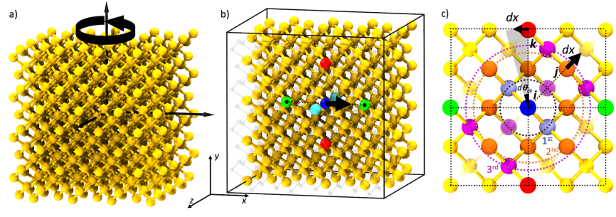
Figure 2: Perturbations on Si structure with $4\times 4\times 4$ conventional diamond unitcells. (a) Rotation of structure around $y$-axis with $\theta$ angle, (b) perturbation of central atom (dark blue) along $+x$ direction (Mixed Perturbation), and (c) radial and tangential perturbations of atoms at neighbouring shells of central atom. In (c), the cross section of the structure along $x$-$y$ plane is shown with 4 conventional surrounding units cells. Only the atoms within 4 layers along $-z$-axis (up to light blue atom in (b)) can be seen in (c). While green and red atoms are 4^th-shell neighbours along $x$- and $y$-axes, grey, orange and purple atoms are neighbours at 1^st, 2^nd and 3^rd shells, respectively. $d\theta_{ijk}$ shows the angle that corresponds to the tangential perturbation $dx$ on the sphere of 4^th-shell neighbours.

Our analyses for the representations are based on the desired features of encoding structural information of the materials that are listed above as invariance, sensitivity, dimensionality, differentiability, interpretability, scalability, complexity, and discrete mapping. While many of these features are important according to the application, we focus here on the invariance, sensitivity, and dimensionality.

Invariance of a representation or a descriptor under symmetry operations such as translation and rotation is of high concern in developing mapping methods since the properties of a material should be identical under these changes of the configuration description. The structural representations are constructed to follow these conditions otherwise every possible transformation of the material must be included in the training of the machine learning model, leading to unaffordable numbers of permutations. Even a successful construction of such a model can lead to undesired predictions for the uncharted permutations that are not in the training datasets.

Sensitivity is also an important property of a descriptor since any application needs distinguishable and unique values for the descriptors. How sensitive the descriptor is to changes in the structure of the material determines the outcome of similarity analysis or molecular dynamics simulations. For example, if a descriptor produces exactly the same values for any perturbation, the outcome will be indistinguishable. In MD simulations, such insensitivity will result in inaccurate dynamics due to inaccuracies in energy and force evaluations as a result of artefacts introduced by the descriptor.

Dimensionality, on the other hand is more related to the under- or over-determination of the feature space for the ML application. While under-determination in the mapping of hyper-dimensional space can easily lead to inaccurate predictions of an ML model, over-determination may also lead to undesired predictions according to how the over-determined features are eliminated.

V.1 Invariance and Sensitivity Analysis

Our analysis of invariance, local stability and sensitivity are carried out using diamond cubic Si structures. All the selected descriptors in this work start from neighbour analysis based on atom-centred perspective, as described in Section III and therefore the descriptors generate values invariant under translational symmetries by definition. However, whether they can maintain invariance under rotation needs to be verified. To evaluate this, we perturbed $4\times 4\times 4$ cubic diamond crystal Si (c-Si) as follows: rotating the structure around the $y$-axis in a non-periodic unitcell, we calculated the difference of descriptors and representations, $dV_{\mathrm{all}}$ from the reference non-rotated structure (see Figure 2a).

For the sensitivity analysis, we perform three types of perturbations to a $4\times 4\times 4$ c-Si unitcell as follows:

1. Mixed Perturbation: the central Si atom with dark blue color in Figure 2b is moved along the [100] direction (i.e. line joining the light green atoms on $x$-axis) within a periodic supercell by a distance $dx$, ranging from $10^{-8}$ Å to $0.1$ Å.

2. Radial Perturbations: The atoms in the groups of 1^st, 2^nd, 3^rd, and 4^th neighbour atom shells at different distances from the central dark blue atom are perturbed along radial and tangential directions (see Figure 2c). For the radial perturbation, atoms in each shell are moved along the vector that separates the atom from the central atom. Position change $dx$ ranges from $10^{-8}$ Å to $0.1$ Å.

3. Tangential Perturbation: Neighbouring atoms in the same shells are perturbed on the sphere inscribed by the distance vector $R_{ij}$ (see Figure 2c). This perturbation only changes angular contributions of the descriptors since the radial distances $R_{ij}$ are kept fixed. Position change ranges from $10^{-5}$ Å to $0.1$ Å.

For case 1, we look at the difference in the full structure representation $dV$ (comprising all atomic descriptors) with respected to the unperturbed crystal to investigate whether the full representation is sensitive to small perturbations of a single atom in the structure. In this mixed perturbation test case, all the neighbor distances for the perturbed central atom change from the perspective of the central atom $i$, and the difference $dV$ from the reference unperturbed structure depends on both radial and angular contributions.

For cases 2 and 3, we look at the difference of the descriptor $dV_{i}$ of the central atom $i$ with respect to an unperturbed neighbourhood. This allows us to test the sensitivity of the individual radial and angular contributions.

V.1.1 Sensitivity to perturbations

We consider the question of whether the representation $V=V(\{R_{ij}\}_{j})$ changes in a locally smooth and stable manner near some reference configuration $\hat{R}=\{\hat{R}_{ij}\}_{j}$. Small changes in the configuration should lead to proportional changes in the representation, a property that we called sensitivity. This requirement is necessary to represent an arbitrary smooth function with the same symmetries and to inherit its regularity, which in turn is key to obtain accurate fits with few parameters or basis functions.

To illustrate this concept, consider a “feature map” $v:\mathbb{R}\to\mathbb{R}$ which is strictly increasing and hence invertible, but assume $v(x)\sim a_{2}x^{2}$ as $x\to 0$. It follows that $x(v)\sim\sqrt{v/a_{2}}$, i.e. the inverse has a singularity. Suppose now that we wish to represent the linear function $f(x)=x$ as $f(x)=g(v(x))$ then $g(v)=f(x(v))=x(v)$, i.e., it inherits the singularity which makes it challenging or even impossible to obtain an accurate fit.

In general, we consider paths $R(t)=\{R_{ij}(t)\}_{j}$ with $R(0)=\hat{R}$ and expand the change in the descriptor to leading order,

$$dV=\|V_{t}-V_{0}\|=a_{k}t^{k}+O(t^{k+1})$$ (30)

for some $k\geq 1$. We call a descriptor $V$ linearly stable $\hat{R}$ if $k=1$ for all possible perturbation paths, i.e., if the change in the descriptor is linear as the perturbation amplitude $t\to 0$. If $k>1$ then we call $V$ linearly unstable at $\hat{R}$.

In our sensitivity analyses we choose different perturbation paths $R_{ij}(t)$ leading to different paths in descriptor space $V_{t}$. From Equation (30) we then obtain

$$\log\|V_{t}-V_{0}\|\sim k\log t\quad\text{as }t\to 0,$$

that is we can observe the stability or instability of a descriptor by analysing the slopes on a logarithmic scale. A linear slope, i.e., linear stability is guaranteed to fulfil our sensitivity requirement. However, in certain high symmetry settings this requirement must be relaxed as we will see in Section VI.1.

V.2 Dimensionality Analysis

The descriptors analysed here are all constructed from feature sets extracted from the structural mapping of the atomic neighborhood density to hyper-dimensional spaces. Their central objective is the requirement to cover all possible perturbations of the structure to ensure a faithful representation to the ML model. However, strictly following this concern can lead to over-determination in the hyper-dimensional space. In other words, the representation may cover only a small subspace of the full hyper-space, with the subspace depending on the parameter set used. In the case of over-determination, feature sequences may contain many zero entries, or, for multi-species systems, may need to be padded with zeros to account for species missing from individual environments. Both of these cases lead to high sparsity in the descriptors, which in principal could be eliminated by carefully selecting parameters to removing unnecessary features from the final descriptor sets and hence from the representations. Moreover, using an over-determined mapping is likely to induce overfitting and noise in subsequent ML training. In ML applications, such non-informative data should be eliminated before the actual training of the model to reduce the error in the training and increase the accuracy of the resulting models.

Due to the well-known curse of the dimensionality, the dimension of the parameter space of a global optimization problem is the key determiner of the difficulty of obtaining optimal solutions. When representations form the input data for an optimization problem, their dimensionality thus has a crucial role in determining complexity. As the dimensionality increases, the number of possibilities rises combinatorially, drastically hindering the task of optimization.

To keep the features at an affordable level for optimization while maintaining an accurate description, one can use dimensionality reduction techniques such as CUR decomposition Imbalzano et al. (2018), farthest point sampling (FPS)Imbalzano et al. (2018), Pearson correlation coefficient (PC) Imbalzano et al. (2018), or principle component analysis (PCA) Cubuk et al. (2017); Onat et al. (2018). While these techniques help to identify the most informative features in the descriptors, they also help to analyse how the features of the descriptors can provide sufficiently informative data through an analysis of its “compressibility”, and whether the representation leads to an over-determined embedding. Here, we have used CUR and FPS as implemented in Ref. 70 as well as PCA to select the optimum number of features for the descriptors.

V.3 Analysis of Dimensionality with Regression

A key question for models based on representations is how the outcome of predictions are depends on the dimensionality of the representation. To assess this, we analysed the model prediction errors of representations on the structures and total potential energies, $E_{\mathrm{DFT}}$ taken from the Si GAP fitting database in Ref. 82. This is a subset of the complete Si dataset used elsewhere in this work, chosen here to allow comparison with results for the same dataset in Refs. 73, 82 and 83. For the target values ${\bf t}$ in Equation 1 we use the cohesive energies, i.e.

$$t_{k}=E_{\mathrm{DFT}}(\chi_{k})-N^{\mathrm{at}}_{k}E_{0},\;k=1\dots N_{k}$$ (31)

where $N^{\mathrm{at}}_{k}$ and $E_{0}$ are the number of atoms in each $\chi_{k}$ structure and the energy of an isolated Si atom, respectively. The cohesive energy of structure $\chi_{k}$ can than be estimated via the linear combination

$$E_{c}(\chi_{k})=\sum_{v=1}^{N_{f}}c_{v}V_{k,v}(\chi_{k})$$ (32)

where the index $v$ runs over all $N_{f}$ features within the representation.

For a global representation of a structure such as in MBTR the ${\bf V}_{k}$ are taken directly as the representation vectors for each structure $\chi_{k}$. For atom-centered descriptors, however, we first construct a global representation by summing over the descriptor vectors for each atom ${\bf V}_{k}^{(i)}$, i.e.

$${\bf V}_{k}(\chi_{k})=\sum_{i=1}^{N^{\mathrm{at}}_{k}}{\bf V}_{k}^{(i)}(\chi_{k})$$ (33)

In both cases we normalised the ${\bf V}_{k}$ representations using the training dataset for each representation method.

The cohesive energies can now be estimated by minimizing the $L_{2}$-regularised quadratic loss function

$$J=\sum_{k=1}^{N_{k}}|E_{c}(\chi_{k})-t_{k}|^{2}+\lambda\sum_{v=1}^{N_{f}}|c_{v}|^{2}$$ (34)

To estimate the coefficients ${\bf c}$, we build two regression models based on (i) linear ridge regression with $L_{2}$-norm regularisation, obtaining the least-squares solution with the QR method (RR) defined in Refs. 73 and 83 and (ii) kernel ridge regression (KRR) as detailed in Ref. 64.

For the linear ridge regression case, the regularised least squares problem becomes

$$\min_{{\bf c}}\|{\bf c}\bm{\Psi}-{\bf t}\|^{2}_{2}+\lambda\|{\bf c}\|^{2}_{2}$$ (35)

where ${\bf t}$ is a vector comprising all the target cohesive energies, ${\bm{\Psi}}$ is an $N_{k}\times N_{f}$ matrix with representations along each rows and structures down each column and $\lambda$ is a regularisation parameter.

For the kernel ridge regression case, we use the ${\bf V}_{k}$ representation to build an $N_{k}\times N_{k}$ kernel matrix with elements

$${\bf K}_{ij}=K({\bf V}_{i},{\bf V}_{j})=\exp\left(-\gamma\||{\bf V}_{i}-{\bf V}_{j}\|^{2}\right)$$ (36)

where $\gamma$ is a lengthscale hyperparameter. After constructing the kernel matrix, one can then predict the cohesive energy for a new configuration with representation ${\bf V}$ as

$$E_{c}={\bf c}\kappa({\bf V}),$$

where ${\bf c}={\bf t}^{T}({\bf K}+\lambda{\bf I})^{-1}$ and $\kappa_{k}=K(\mathbf{V}_{k},\mathbf{V}).$

VI Results and Discussions

VI.1 Sensitivity

VI.1.1 Sensitivity to Rotations

In Figure 3, we present the norm of the difference vector $dV$ between the full structure representations of the rotated and the reference c-Si system for each approach considered.

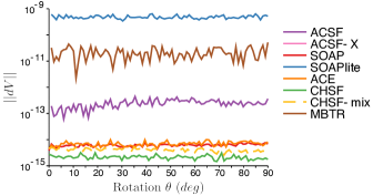
Figure 3: The norm of the difference in representation values between the reference structure and rotated whole structure by an angle $\theta$.

Our analyses show that all descriptors maintain the rotational invariance with high precision, with all errors below 10^-9 (above machine precision $\epsilon$ of $\sim 10^{-16}$). Together with built-in invariance with respect to translations and permutation of like atoms of all the representations based on density projections, our analysis indicates that all approaches considered in this work fulfill the properties of invariance in rotation, translation and permutation for the structural representations.

Considering the wide range of outcomes on the rotation tests, we ascribe the error to the numerical precision differences i.e. floating point roundoff error of the underlying codes. For the sake of comparison of the outputs from different approaches considering the numerical precision of underlying codes, we selected $10^{-8}$ as the lower bound in all our subsequent sensitivity analysis following the lowest precision observed in these rotation tests.

VI.1.2 Sensitivity to Perturbations

Further analyses are carried out for the sensitivity of representations under the atomic motions in structures as described in Section V.1. Recall from Section V.1.1 that a slope of one indicates local stability (and smooth invertibility of the descriptor) while a slope greater than one leads to singularities in the representation.

Figure 4 shows the results for the Mixed Perturbation with representation changes $\|dV\|$ normalised so that all curves pass through the point (0.1, 0.1) to enable direct comparison. This lets us to provide an absolute comparison for $\|dV\|$ metric between reference and perturbed structures. All representations have linear sensitivity within the entire range of the path, except for MBTR which shows a mild preasymptotic sign of instability (change of slope from 1 to 2 above $0.01$ Å), which is unlikely to cause any significant deterioration in stability of the representation. This is apparent here since MBTR is a global representation method. Compared to other atomic descriptors, the results for MBTR show that its histogram of angles leads to a smooth change in the slope. In the atomic descriptors, this calculation includes contributions from all descriptors hence the slope is dominated by radial contributions, which are discussed detailed in next section.

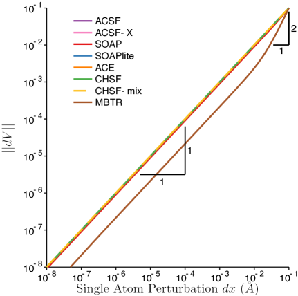
Figure 4: The norm of the difference in representation values between the reference structure and c-Si with perturbation of a single-atom by a distance $dx$, corresponding to the Mixed Perturbation in Section V.1.

Figure 5: Norm of difference of atomic descriptors on atom $i$ as a neighbouring atom $j$ is perturbed from its reference position. (a) Radial perturbation and (b), (c), and (d) tangential perturbations as shown in Figure 2c. The tangential perturbations (b) in a high symmetry direction for 1^st shell, (c) in a random direction for 1^st shell and (d) in a random direction for 2^nd shell with random radial perturbations on the same shell before applying tangential perturbation on one of the same shell atom. In (b) and (c), no radial perturbation is applied before the tangential perturbations.

VI.1.3 Radial perturbation of reference crystal

A deeper analysis of the sensitivity of representations can be made by analysing the responses of the atomic descriptors to different perturbation modes. As described in Section V.1, we calculated the change in the descriptor of the central atom $i$ to a radial perturbation of a neighbour $j$ as shown in Figure 2c. The sensitivity curves corresponding to the radial perturbation of a neighboring atom in the 4^th shell are given in Figure 5a. All descriptors have slope-1 sensitivity curves, indicating linear stability under this perturbation. This is unsurprising since all descriptors provide a relatively high resolution of the 2-body histogram.

VI.1.4 Tangential perturbation of reference crystal

Next, we repeat the test of the foregoing section with a tangential perturbation of an atom in the 1^st shell. The resulting sensitivity curves are given in Figure 5b, clearly showing slope 2 for all descriptors. Thus, according to Section V.1.1 all descriptors are unstable with respect to tangential perturbations, raising concerns due to the resulting singularity in the inverse of the descriptor map. However, the origin of this instability is invariance with respect to reflections about a plane, and fitting any target function with the same reflection symmetry need not be affected by the singularity in the inverse descriptor map.

Concretely, let $i$ denote the centre atom and $k$ the neighbour that is being perturbed in the tangential direction, i.e.,

$$R_{ij}^{t}=R_{ij}^{0}+tdR_{ij}+O(t^{2}),$$

where $dR_{ij}=0$ for $j\neq k$ and $\|dR_{ik}\|=1$ and $dR_{ij}\perp{R}_{ij}^{0}$. If $R^{0}$ is symmetric under reflection through the plane that contains the origin and is orthogonal to $dR_{ik}$ (this is the case here) then the configuration $R^{-t}$ is the reflection of $R^{t}$ to within $O(t^{2})$ accuracy. Since all descriptors $V$ we consider are invariant with respect to reflections they necessarily satisfy $\frac{d}{dt}V^{t}|_{t=0}=0$ (this is true for any function of the distances $r_{ij}$ and the cosines $A_{ijk}=\cos\theta_{ijk}$), and hence $V^{t}\sim a_{2}t^{2}$ as $t\to 0.$ In particular, the inverse descriptor map $V\mapsto R$ must contain a square-root singularity along the path $V^{t}$.

On the other hand, assume we aim to represent a property, e.g., site potential, $\epsilon=\epsilon(\{R_{ij}\}_{j})$, then $\epsilon$ will also satisfy this reflection symmetry, which indicates that the square-root singularity is again removed. To illustrate this point further we modify the one-dimensional example from Section V.1.1: Assume that we wish to represent $f(x)=x^{2}=g(v)$, then $g(v)=f(x(v))=x(v)^{2}\sim v/a_{2}$ as $v\to 0$, i.e., the singularity is removed in this case. More generally, this occurs whenever $f(x)\sim b_{2}x^{2}$ as $x\to 0$, i.e., when $f$ is symmetric about the origin to leading order.

VI.1.5 Tangential perturbation of a perturbed crystal

The analysis of the previous paragraph suggests that any perturbation in the configuration of the structure that breaks the symmetry should lead to the linearly stable slope-1 cases. We therefore test which descriptors are capable of capturing this symmetry breaking. We break the symmetry in several ways: we perturb an atom in a random tangential direction; we perturb atoms in the second shell which doesn’t exhibit the same reflection symmetry; and we perturb the reference crystalline structure in the radial direction from a chosen centre atom $i$, before applying these tangential perturbations. The results are shown in Figure 5b–d.

As predicted, any such symmetry breaking leads to changes in the slopes of sensitivity curves of descriptors in the limit $t\to 0$. However, there are differences across descriptors how well the symmetry breaking is captured. First, there are some variations across descriptors how significant the pre-asymptotic slope-2 regimes are, which indicate a reduced sensitivity. However, the most concerning effect is the “dip” in the CHSF descriptor in Figure 5c, highlighting a region of significantly reduced sensitivity (it can almost be thought of as blindspot) for atomic displacements in the descriptors, where the perturbation does not change the output values of representations. To test whether adding additional features can remove this dip we implemented an extended CHSF descriptor, labelled CHSF-mix, for which the radial and angular histograms are fully mixed giving a similar description of the 3-body histogram as SOAP and ACE do. This addition clearly removes the reduced sensitivity regions.

VI.2 Dimensionality of Representations

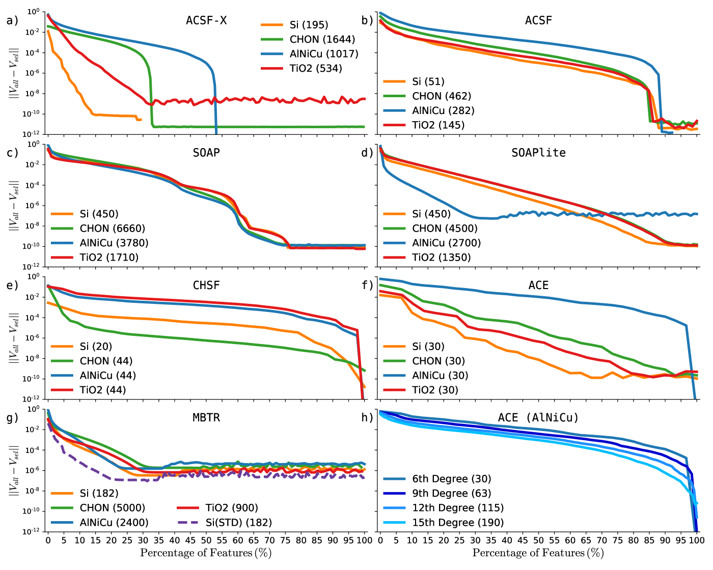
Figure 6: CUR decomposition based dimensionality reduction analysis of (a) ACSF-X, (b) ACSF, (c) SOAP, (d) SOAPlite, (e) CHSF, (f) ACE, and (g) MBTR representations with four datasets that are indicated in legend with the number of features of each within parentheses. Figures show the error in the representation from the non-reduced feature set as a function of the percentage of features selected. Legends show the corresponding datasets of Si, CHON, AlNiCu, and TiO₂ while in panel (g) Si(STD) shows the standardized representation output for Si dataset and in (h) the legend shows the results of ACE with different polynomial degrees from 6 (as used in panel (f)) to 15 for the AlNiCu dataset.

In the second phase of our analyses, we consider four different datasets selected from those described in Section IV, namely Si, CHON, AlNiCu, and TiO₂. Each dataset contains a diverse range of configurations with thousand of structures. To identify how the dimensionality of the representations change with different datasets using the same parameters, we used CUR and FPS feature selection techniques and analysed the reduced dimensions of the representations by comparing them with the outcomes of PCA calculations. This analysis can also be accounted as a measure of the compressibility of each representation.

Table 1: Number of features for each representation in different datasets. The numbers in parentheses show the full feature set before non-zero elements are selected.

Desc.	Si	CHON	AlNiCu	TiO2
ACSF	51	462	282	145
ACSF-X	57(195)	634(1644)	544(1017)	534
SOAP	450	6660	3780	1710
SOAPlite	450	4500	2700	1350
CHSF	20	44	44	44
ACE	30	30	30	30
MBTR	182	5000	2400	900

VI.2.1 CUR decomposition

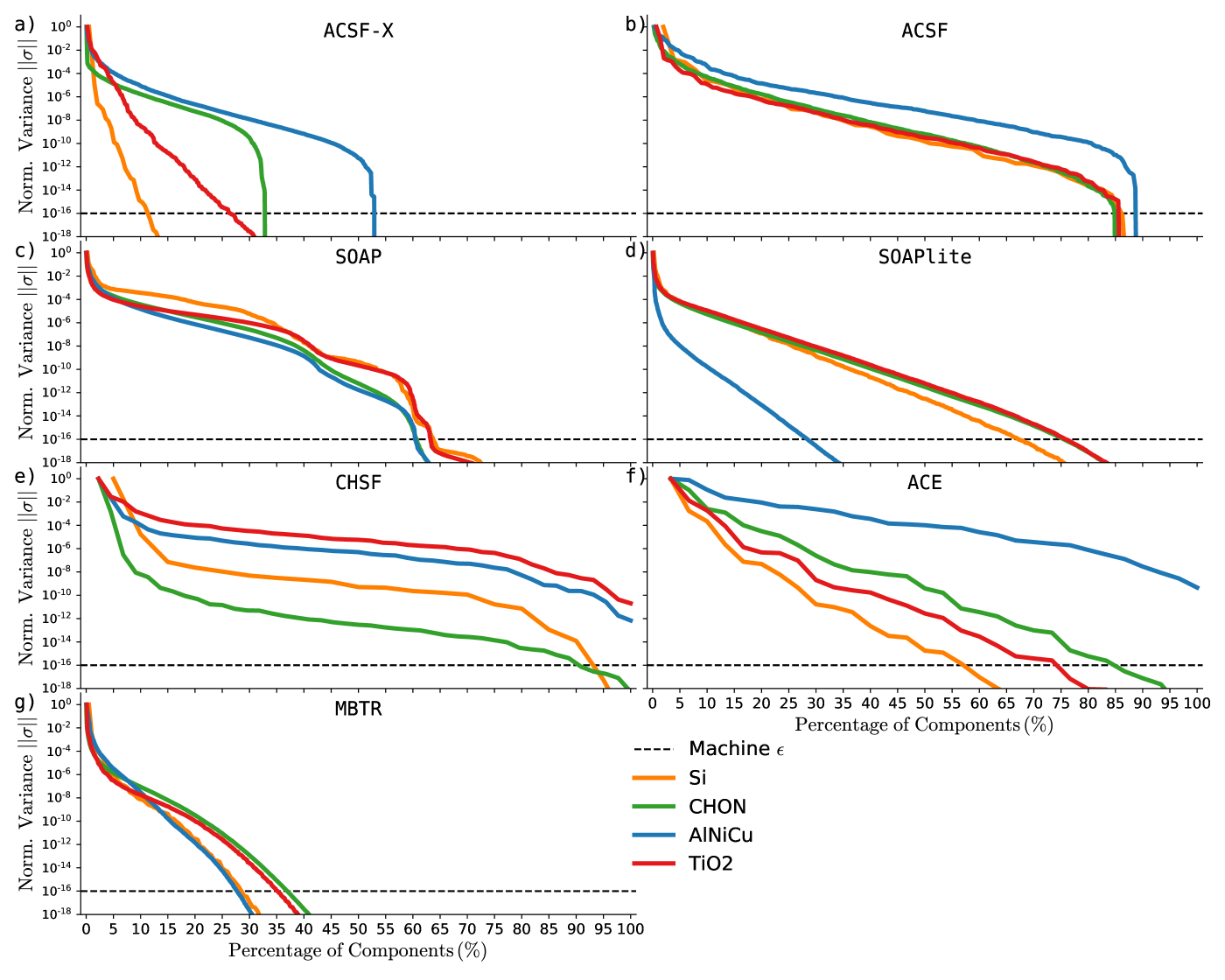
Figure 7: The variance of features versus the percentage of the selected components of (a) ACSF-X, (b) ACSF, (c) SOAP, (d) SOAPlite, (e) CHSF, (f) ACE, and (g) MBTR representations using PCA analysis. Different colors show results for each representation with selected datasets. The dashed black and blue lines show the machine precision and the lower bound in our variance analyses where any value below this threshold is treated as zero.

As a first step we analysed the representations including all element-wise descriptors. MBTR is considered as a representation-only approach as its output cannot be broken down to element-wise descriptors. In Figure 6, the total error between the full feature sets of each dataset and the reduced feature sets that are extracted from CUR analysis is presented. As each approach provides a different number of features for the datasets at hand depending on the selection of (hyper)parameters, we provide a complete list of the number of non-zero features in each representation with the corresponding datasets in Table 1 and in the legends of each panel of Figure 6.

After removing any features of ACSF-X that are all zero from Si and AlNiCu dataset (see Figure 6a), the selection method CUR in Section V.2 is applied throughout the dataset and features from the full feature set are selected one-by-one and added to the new feature set by calculating the error with respect to the full feature representation. Using this method, the features that contribute most to the representation can be selected. As the lower contributions are added to the new feature set, the error cannot be reduced more and the overall error becomes constant, equal to zero within numerical precision. The number of features that are selected at the beginning of this plateau can be counted to determine the size of the compressed representation, and conversely the number of remaining features can be thought of as the over-determination of the representation.

In Figure 6, one can see three types of results: (i) those with error curves that gradually decrease to the point where the error plateaus as for the TiO₂ results of ACE, ACSF-X and MBTR; (ii) errors decrease step-wise to a plateau such as in SOAP results; and (iii) where errors drop rapidly as for the AlNiCu results in ACSF, ACSF-X, ACE and CHSF.

SOAP and SOAPlite, in Figure 6c and d, respectively, can be directly compared since they differ only in the choice of radial basis function. The results for the Si, CHON, and TiO₂ datasets can be examined for both approaches. While SOAPlite has close to exponential decay up to $\sim$70% of selected features, in SOAP this regime extends only up to 30%. After this, the SOAP error has a more step-like character. Similar behaviour can also be seen in type (iii) results such as ACSF, ACSF-X, CHSF, and ACE. For these methods, while the first $\sim$10% of features vary the error reduction, the rest of the features only slightly reduce the error. For the AlNiCu dataset, SOAP and SOAPlite have substantially different outcome from the rest of the datasets which is an indication on how the choice of radial basis can be a key determiner for the relevance of features in the representations. One can also see the dominance of radial basis in the global representations when Figure 4 is compared with Figure 5. The optimal choice of basis functions for descriptor performance is another open question and is outside the scope of present work. We leave further investigation of basis functions’ role on the sparsification and descriptor performance for future work.

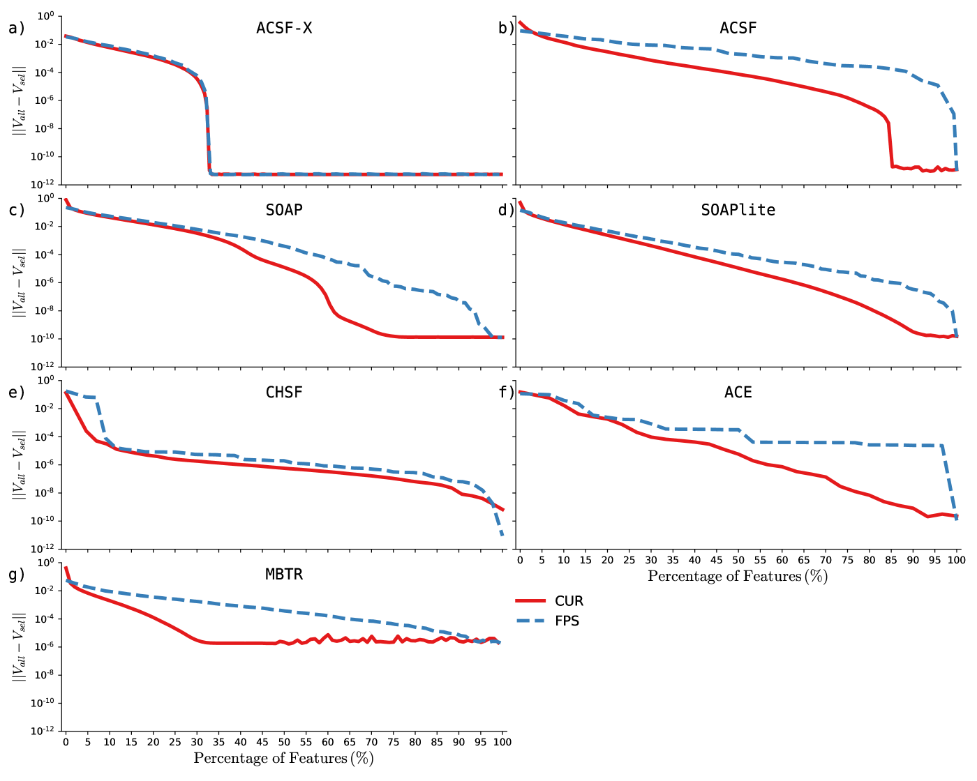
Figure 8: Comparison of CUR and FPS based dimension reduction analysis on ACSF both with (a) extended and (b) standard parameter sets, (c) SOAP, (d) SOAPlite, (e) CHSF, (f) ACE, and (g) MBTR representations for CHON dataset.

In most of our dimensionality reduction results, one can see distinct constant error regions associated with over-determination. These features should ideally be eliminated before using the representation in ML models. For example, consider the results for ACSF-X and ACSF in Figure 6 a and b. As the aim of ACSF-X is to extend the number of features in set from the widely-used and well-tested standard ACSF parameter set, some of the features are expected to be irrelevant for representing structures in our datasets. It is thus unsurprising that the dimension reduction analyses in Figure 6a show that there only fractions of features contribute significantly - around 14% for Si, 33% for CHON, 54% for AlNiCu, and 33% for TiO₂. A smoother feature reduction can be seen for the standard ACSF parameter set in Figure 6b, where the error decay is very similar with about 85% of the total features sufficient across all four datasets and thus around 15% of redundant features.

A similar result is seen for SOAP, where around 75% of the features of SOAP representations are sufficient to cover the structural variance across all datasets. This result is more striking than that for ACSF since SOAP has about an order of magnitude more features in its representation. We can conclude that both ACSF and SOAP are robust approaches that cover the hyper-dimensional space of structural representation for a wide-range of crystals and molecules.

The ACE AlNiCu results are significantly different than the other datasets. To identify whether the degree of the polynomial is the reason for this pattern, we carried out additional analyses with ACE, increasing the degree of polynomial from 6th to 15th degree in steps of 3 degrees, as shown in Figure 6h. Increasing polynomial degree significantly increases the number of features; however, we find that the percentage of selected features on the final representation does not change significantly and the pattern of error decay is still quite different from the rest of the datasets (e.g, Si, where 25% of the features can be removed from the representation although it has order of magnitude less features in the descriptor vectors than with 15th degree of polynomial expansion.

To further investigate the extensive redundancy identified for MBTR features across all four datasets, we consider whether the discretised smearing of positions and angles used by the MBTR representation leads to clustering of the features representation space. To identify any clustering of the data, we perform standardization of the features for all the representations of Si that are generated by MBTR and show the feature selection curve in Figure 6g labelled as Si(STD). When compared with Si curve, Si(STD) does reduce the error when less than $\sim$20% of features are selected by around an order of magnitude in comparison to the raw representation. However, standardization suggests an even smaller feature set selection of about only 20% of the full feature set. This may be due to the Gaussian smearing with $D$ in MBTR that significantly increases the correlation between features.

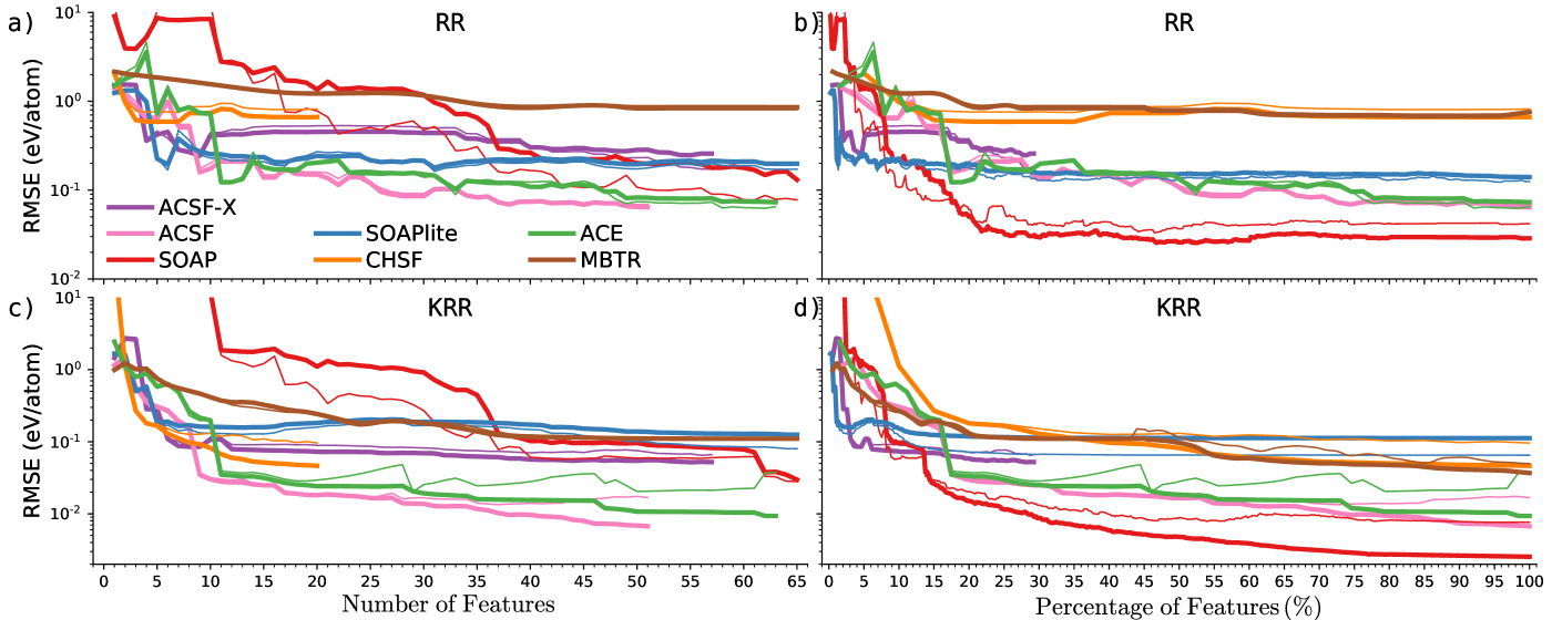
Figure 9: Comparison of RMSE using (a),(b) RR and (c),(d) KRR with Si dataset on representations while (a) and (c) showing up to the top 65 features that are selected with CUR method. Thick lines represent training errors, thin lines represent test errors.

VI.2.2 Principal Component Analysis

The CUR selection process is closely related to the principle components of the representation data for each dataset. To show whether these principle components are related to the final feature selections in CUR, we further analysed the datasets using PCA. In Figure 7, the fraction of variance explained by the principle components of the four datasets are given for each representation. Since the PCA variances decrease from one to very small values, we determine a lower bound after which we consider the variance to be zero, shown as the zero level in our figures. PCA variation results for principle components follow the same trends as the CUR curves discussed above. Although CUR results show directly the hyper-dimensional space of the representation, PCA results are not solely based on the selected features but are a collective property of all features based on the covariance matrix from which the principle components are extracted. As seen in Figure 7, the outcome of this selection following the highest to lowest variances and extraction of the features with highest values in the covariance matrix gives similar results to the CUR decomposition.

VI.2.3 Farthest Point Sampling

CUR and PCA are both based on SVD decomposition, selecting the features as orthogonal dimensions of the hyper-dimensional space, treating each feature as linearly independent since linearly dependent features cannot span the space. However, neither of these methods consider if the selected features have non-linear dependencies on other features. Another approach to select features without using SVD decomposition is Farthest Point Sampling (FPS). In FPS, the feature selected at each iteration is chosen as the farthest from those already selected. Hence, FPS does not provide information on whether the selected feature is indeed linearly independent to those already selected. This can be understood by considering each features’ distance from the others at a time late in the process when there are few remaining features to be selected. These remaining features either represent very small distances as minor additions to the previously selected and clustered features or repeat similar distances.

In Figure 8, the FPS results for the feature selection show that there are significant differences in error reduction and hence dimension compression for SOAP, SOAPlite, ACE and MBTR representations in comparison to our earlier CUR results. However, these FPS results do not allow insight into each features’ contribution as a dimension in the hyper-dimensional space. The relatively small reduction of errors in FPS selection or the constant regions are due to its selection criteria, which is based only on hyper-spatial distance. This poses a limitation in the analysis if one would like to find the full extent of the representation and remove non-informative features from the descriptors. However, determining the cutoff for the features according to the error is not obvious since there may not be a plateau in the error — as is seen for in ACSF-X, where only 25% of features contribute — but instead a more gradual decrease as in the results for all other representations.

VI.3 Regression with Representations

The RR and KRR methods are applied to all representations using subset of Si dataset (see Section V.3) and RMSE is calculated as a function of the number of features in each representation.

For each representation, the regularisation parameter $\lambda$ used in both RR and KRR methods and the $\gamma$ hyperparameter of ${\bf K}$ in KRR were chosen to optimize the convergence of the RMSE in the predictions on an independent test set.

In Figure 9, we present our regression results for the two ridge regression methods RR and KRR in the first and second rows of the figure, respectively. While RMSE of both training (thick lines) and test datasets (thin lines) are shown in Figure 9a and c for each regression method and for the top 65 features that selected by the CUR method, the RMSE of full feature extension of representations are provided for comparison in Figure 9b and d.

Our intention here is not to provide the best potential energy surface (PES) estimator for each representation method, since this has already been extensively studied in the literature but instead to provide a common metric to compare different representations. Here by fitting those methods to same dataset, we can assess how each method performs under this task, and in particular how the dimensionality of each method effects the outcomes.

The effect of the dimensionality of the feature space can be seen from the RR outcomes of representation for the full feature set. In Figure 9b, one can identify plateaus at three typical RMSE values: 0.9, 0.1, and 0.04 eV/atom. While RMSE for both training and test dataset of SOAP has the highest accuracy with 0.04 eV/atom, MBTR and CHSF have the lowest accuracy of around 0.9 eV/atom. The rest of the methods have final errors of around 0.1 eV/atom. As the ridge regression is a linear fit to representation features, the RMSE can be compared directly between methods. The results indicate that SOAP has enough features to cover the structural variation but convergence is slow using a linear fit. However, using a non-linear fit as in Figure 9d outperforms RR. While SOAP has still the highest accuracy, albeit with a significant split of RMSE between test and training datasets, ACSF, ACE, and SOAPlite result in predictions that are at least an order of magnitude higher in accuracy in KRR than in RR.

To identify the role of the most important features in each representation on the prediction RMSE, we analysed the RMSE of methods while only using the top-ranked selected features from CUR up to 65 features. The RMSE of RR shows that ACE and ACSF have very similar results up to 50 features, where they reach an accuracy comparable to that of 65 features with the SOAP or SOAPlite models. When non-linearity is introduced in the KRR models in Figure 9c the difference is even more stark, for example CHSF with only 20 features has comparable accuracy with SOAP at 65 features.

These results raise the question: what is the best feature set for a given representation, or equivalently, what is the necessary dimensionality for a given representation for a specific dataset or material? In Figure 9d, we can see that RMSE of training and test datasets for SOAP and ACSF start to diverge at about 50%, and 70% of features, respectively. These points coincide with the region in Figure 7 where the variance of these representations drops below about $10^{-12}$. Similar results can also be observed from the KRR results for MBTR, CHSF, and ACE where either RMSE does not reduce more with the addition of new features such as in ACE beyond 45% features, or RMSE of test dataset significantly increases as in MBTR after 40% features are selected.

These results show that there are clear inconsistencies between the selections of features in representation and even within the same representation as two critical points need to be considered before applying a feature set to MLIPs using dimension reduction: 1) the number of features may not be indicative of complete coverage of structural representation of a method, 2) increasing the number of features may not result in gaining benefit and may also cause overfitting.

VII Conclusion

We have carried out a comprehensive assessment of the sensitivity of atomic environment representations, using several methods to analyse the sensitivity under rotation and various perturbations. Our results show that although many representations provide an overall acceptable accuracy for sensitivity, there is still room to balance sensitivities to radial and angular perturbations. We thus conclude that further investigation of how insensitivities effect applications of interatomic potentials and hence observables in MD simulations is necessary to improve ML driven simulation approaches.

We also carried out extensive dimensionality analyses of various representations, which have identified significant opportunities to eliminate unnecessary information that may reduce the accuracy of predictions from ML models. We also conducted regression tests to provide a comparison between representations as their dimensionality varies. The results show clear differences in the number and fraction of important dimensions in the different representations. This is expected to become increasingly important as more complex representations are developed, and especially when incorporating property-based descriptors alongside atomic environment representations.

VIII Data Availability Statement

The data that supports the findings of this study are openly available in github.com/DescriptorZoo/Materials-Datasets at http://doi.org/10.5281/zenodo.3871650, Version v1.0 that are extracted from open-access NOMAD Archive (http://nomad-coe.eu)DAT (2020). The details of all datasets are given at Section IV. The corresponding citations for other data that are used in this study are available from the following publications: GAP Si potential database from Ref. Bartók et al. (2018), Si molecular dynamics (MD) database from Ref. Cubuk et al. (2017) and TiO₂ dataset from Ref. Artrith and Urban (2016) through web access from Ref. ann.atomistic.net/download/ (2019). The codes that are used to create representations are detailed at Section III.8.