Accelerating ultrafast spectroscopy with compressive sensing

Abstract

Ultrafast spectroscopy is an important tool for studying photoinduced dynamical processes in atoms, molecules, and nanostructures. Typically, the time to perform these experiments ranges from several minutes to hours depending on the choice of spectroscopic method. It is desirable to reduce this time overhead to not only to shorten time and laboratory resources, but also to make it possible to examine fragile specimens which quickly degrade during long experiments. In this article, we motivate using compressive sensing to significantly shorten data acquisition time by reducing the total number of measurements in ultrafast spectroscopy. We apply this technique to experimental data from ultrafast transient absorption spectroscopy and ultrafast terahertz spectroscopy and show that good estimates can be obtained with as low as 15% of the total measurements, implying a 6-fold reduction in data acquisition time.

I Introduction

Ultrafast spectroscopy has found a wide range of applications to study time-resolved ultrafast dynamical processes Maiuri et al. (2019); Hunt (2009); Reid and Wynne (2006); Berera et al. (2009); Kraus et al. (2018). Many techniques have been developed spanning different time and photon energy ranges, including ultrafast transient absorption spectroscopy, time-resolved photoelectron spectroscopy, multidimensional spectroscopy, and terahertz spectroscopy Shah (2013); Weiner (2011). These techniques can be very time consuming with acquisition times varying drastically depending on the method. Reducing the time overhead is important, not only for efficiency, but also for making it possible to examine specimens which degrade quickly due to prolonged exposure to a laser beam.

Here we show how to significantly shorten the duration of ultrafast spectroscopy with compressive sensing. We apply compressive sensing to two important ultrafast techniques: ultrafast transient absorption spectroscopy and ultrafast terahertz spectroscopy. The specimen chosen for the transient absorption is a 50 nm diameter colloidal TiN nanoparticles in water, which are of growing interest as refractory metal nanostructures resistant to heat or optical damage for plasmonics applications Guler et al. (2015). This specimen was chosen due to its high degree of optical scattering which makes it extremely challenging and very time consuming to acquire data with reasonable signal to noise ratio. For our experiment, the data acquisition time was about four hours. For ultrafast terahertz spectroscopy, measurements were performed on a methylammonium lead iodide (MAPbI₃) thin film that was spin casted on quartz. This material class is of interest for solar energy conversion and is believed to exhibit long carrier lifetimes owing to low frequency lattice deformations that may help screen charges. The data acquisition for full 2D time-resolved THz experiment took about seven hours to complete, and could require more time for higher signal to noise ratio. These conditions challenge the stability of both laser systems and many specimens. To overcome these difficulties, we show that by taking sparse, random measurements in time, thereby taking a fraction of the total measurements compared to conventional experiments, compressive sensing can faithfully reconstruct the full experimental result.

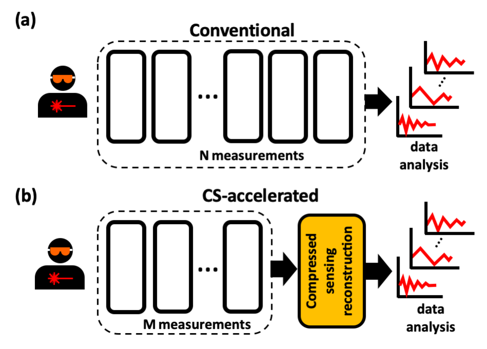
Figure 1: Comparison between conventional and CS-accelerated experiments. (a) shows a conventional experiment which requires $N$ measurements for the fully resolved result. (b) shows the CS-accelerated scheme with $M<<N$ measurements to yield an estimate of the fully resolved result.

II Compressive Sensing for Ultrafast spectroscopy experiments

Recently, there has been wide interest in using different techniques to speed up optical experiments Cortes et al. (2020); You et al. (2020); Kudyshev et al. (2019); Howland et al. (2011); Simmerman et al. (2020). Compressive Sensing (CS) is one such technique for efficiently acquiring and reconstructing signals Baraniuk (2007a); Candès and Wakin (2008); Donoho (2006); Candes et al. (2006); Baraniuk (2007b). It has successfully been applied in many fields, including magnetic resonance imaging (MRI), fluorescence microscopy, multi-dimensional nuclear magnetic resonance (NMR) spectroscopy, quantum imaging, and quantum tomography Sun et al. (2016); Studer et al. (2012); Kazimierczuk and Orekhov (2011); Howland and Howell (2013); Katkovnik and Astola (2012); Shabani et al. (2011); Gross et al. (2010); Zerom et al. (2011); Katz et al. (2009); Wen et al. (2020). CS has also been used in multidimensional spectroscopy for applications in chemistry with impressive speed-ups shown Andrade et al. (2012); Sanders et al. (2012); Dunbar et al. (2013). We propose compressive sensing for material science and condensed matter physics where a different set of ultrafast spectroscopic methods are used, such as transient absorption and ultrafast terahertz spectroscopy. We hope that our work helps bridge the gap between the CS community and the ultrafast spectroscopy community where advanced algorithmic methods are not commonly used.

Generally, the number of measurements, $N$, to capture full information of a signal is determined by the Nyquist-Shannon sampling theorem: the sampling rate should be at least twice the highest frequency of the signal, 2$f_{max}$ Cover and Thomas (2012). If some maximum time $T$ is required to observe the dynamics or infer a spectrum of a given resolution, then $N$ = $T/\Delta t$ = $2f_{max}T$ total measurements would be needed, with $\Delta t$ being the time between measurements (inverse sampling rate). This latter analysis is correct if one only has an upper limit for $f_{max}$ and no other knowledge about the signal. CS overcomes this limit by invoking a sparsity assumption of the signal in some known basis. When a signal is transformed to this basis, most of the coefficients are negligibly small. The existence of such a basis can be used to significantly reduce the total number of measurements required to reconstruct the full signal. Many natural signals are sparse in the Fourier domain. Since time-domain signals are usually real, the discrete cosine transform (DCT) is widely used for compression and CS reconstruction. Other transformations, such as Haar, total variation (TV) and Hadamard transformations are also widely used Howland et al. (2011); Soldevila et al. (2013); Li (2010).

CS reconstructs a signal by solving the convex optimization problem,

$$\min_{\tilde{x}}||\tilde{x}||_{1}\;\text{subject to}\;A\tilde{x}=y.$$ (1)

Here, $\tilde{x}=\psi x$ is the $N\times 1$ sparse solution vector and $\psi$ is the transformation matrix that takes the signal $x$ (e.g., transient absorption), to a sparse basis. We use the DCT, Haar and Hadamard transformations as possible choices for $\psi$. $||.||_{1}$ is the $l_{1}$ norm, i.e., the sum of the absolute values of the components of $\tilde{x}$. The most sparse solution is given by minimizing number of nonzero components of the solution vector $\tilde{x}$ or $l_{0}$ norm. However, $l_{0}$ minimization is non-convex and falls under NP-hard computational complexity which is very difficult to solve. $y$ is the $M\times 1$ vector representing the small number ($M\ll N$) of random measurements taken in the experiment. $A=\phi\psi^{-1}$ is a $M\times N$ matrix, with $\phi$ representing an $M\times N$ random measurement matrix, which we take to be a submatrix of the $N\times N$ identity matrix with $M$ rows chosen randomly. For a $K$-sparse signal, having $K$ nonzero coefficients, the above optimization problem is able to faithfully reconstruct the signal with approximately $K\log{\big{(}\frac{N}{K}\big{)}}$ measurements with high probability. Remarkably, it has been shown that no reconstruction algorithm can reconstruct the signal with substantially fewer measurements Donoho (2006). Additional details of this algorithm are specified in the methods section.

To see why the CS is well suited to ultrafast spectroscopy, consider a pump-probe framework, typical of many such experiments. A short pump pulse centered at time $t_{0}$ excites a specimen and a probe pulse at various later times $t$ = $t_{0}+\tau$ is used to measure the evolution of some material response, $\mathcal{R}$ (e.g., absorbance or transmittance) Weiner (2011):

$$\mathcal{R}(\tau)=\mathcal{R}_{-\infty}+\Delta\mathcal{R}(\tau),$$ (2)

where $\mathcal{R}_{-\infty}$ is the material response prior to the pump. Many measurements are taken at various probe time delays $\tau$, giving information about the full dynamics. Such ultrafast experiments can be time consuming due to the need of making repeated measurements with small increments in $\Delta\tau$. CS is ideally suited for ultrafast optics because in a wide variety of material systems, $\mathcal{R}(\tau)$ is often dominated by a small number, or small range, of frequencies, implying the existence of a sparse basis. For many systems, the total number of measurements taken in conventional ultrafast experiments far outweigh the actual number of measurements, $\sim K\log{\big{(}\frac{N}{K}\big{)}}$, required by CS theory. Here, we test the performance of CS signal reconstruction for two protypical experiments: ultrafast transient absorption and ultrafast terahertz spectroscopy.

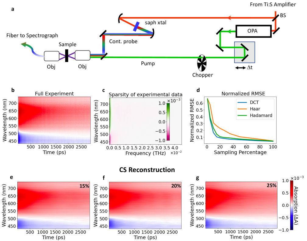
Figure 2: Ultrafast transient absorption spectroscopy. (a) is a schematic of the experimental setup. (b) is the observed change in absorbance across different wavelengths. (c) demonstrates that the full experiment data is very sparse in the DCT domain. Almost all the information is contained in about 5% of the frequency coefficients. This allows CS to reconstruct signals with fraction of the measurements of a conventional experiment. (d) is the NRMSE for DCT, Haar and Hadamard as a function of sampling percentage. (e), (f) and (g) shows the CS reconstruction with 15%, 20% and 25% samples, respectively.

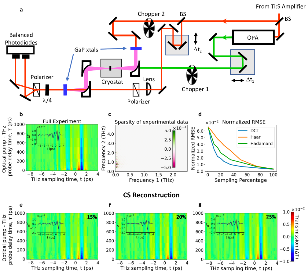
Figure 3: Ultrafast terahertz spectroscopy. (a) shows the schematic of the experimental setup. (b) is the full experimental result. (c) shows the sparsity of the signal in DCT domain. Almost all the information is contained in about 7% of the frequency coefficients. This allows CS to reconstruct the full signal with fraction of the measurements of a conventional experiment. (d) is the comparison of normalized RMSE for DCT, Haar and Hadamard as a function of sampling percentage. (e), (f) and (g) shows the CS reconstruction with 15%, 20% and 25% samples, respectively.

III Results

III.1 Ultrafast Transient Absorption Spectroscopy.

An ultrafast transient absorption spectroscopy is a pump-probe experiment in which a specimen is excited with a femtosecond pump pulse, followed by a probe pulse with a variable time delay. The change in transmittance or absorbance over various time delays are measured giving information about the properties of the specimen. Transient absorption spectroscopy has been used to characterize an extraordinarily large range of photoinduced dynamical processes ranging from molecular excited states, electronic transitions in nanoparticles, plasmonics, charge separation and transport phenomena, to name just a few Wang et al. (2014); Pendlebury et al. (2011); Grancini et al. (2011).

A schematic of our ultrafast transient absorption spectroscopy experiment is shown in Figure 2-a. The output of an amplified femtosecond laser system (Spectra Physics Tsunami and Spitfire) operating at 5kHz and 800 nm pumps an optical parametric amplifier (OPA) to create wavelength tunable 130 fs pulses. A small portion of the 800 nm amplified light (5%) is focused into a thin (2mm) sapphire crystal to create a continuum probe. The pump beam is chopped at half the repetition rate to create “pump-on” and “pump-off” such that a transient absorption signal can be measured with each pump pair. With variable delay of the probe relative to the pump, time-resolved transient absorption spectroscopy can be acquired. The pump and probe beams are focused and spatially overlapped in the specimen (TiN nanoparticles in waters). The probe light is then sent to a spectrograph where the full continuum in the visible spectral range is measured simultaneously for each delay. For this data, each delay required tens of thousands of transient absorption pump-pair measurements. The full data acquisition took four hours due to the high scattering of the colloidal nanoparticle specimen. Next, we show how CS can drastically shorten the duration of experiment.

Figure 2-b is the full experimental data showing the change in absorbance ($\Delta A$) across different wavelengths. It can be seen that $\Delta A$ varies with wavelength. The data indicate a strong transient response of the TiN plasmon absorption following photoexcitation. Since the transient absorption measurement is a difference measurement, it is possible to get positive (an absorption with less light transmitted through the specimen) and negative transient absorption signals (typically a bleach of the ground state absorption, with more light transmitted through the specimen), particularly when there is a spectral shift in the excited nanostructure. In Figure 2-b, the data indicate that the plasmon resonance of the TiN nanoparticles, centered at  520 nm, redshifts upon photoexcitation. For the wavelengths on the lower energy side of 520 nm, more light is absorbed as the peak absorption moves to the red, while the specimen begins to transmit more light at wavelengths on the blue side of 520 nm as the peak absorption moves further to the red away from those wavelengths. Figure 2-c shows the sparsity of the full experimental data for each wavelength in DCT domain. We can clearly see that the signal is sparse with almost all of components concentrated near zero frequency. In fact, only about 5% of the frequency coefficients contain almost all the information about the signal. This suggests that CS can reconstruct the signal with about 15% of the measurements of a conventional experiment. Figure 2 (e-g) shows the CS reconstruction at 15%, 20% and 25% respectively. Qualitatively, all these CS reconstruction looks very similar to the full result in Figure 2-b. This also corroborates our assumption that about 15% measurements of a conventional experiment is sufficient to reconstruct the full experimental signal. To quantify the overall signal reconstruction, we compare the normalized root-mean-square-error (NRMSE) for different sampling percentages in Figure 2-d. We also compare the DCT with Haar and Hadamard transforms. The DCT performs best among these transformations, followed by Hadamard and Haar transforms. It is interesting to note that the NRMSE drops quickly and does not change much from 15% to higher sampling percentage. This suggests that the number of measurements as low as 15% of a conventional experiment is sufficient for a fair reconstruction of the signal.

III.2 Ultrafast Terahertz Spectroscopy

Ultrafast Terahertz spectroscopy is another useful technique for investigating specimens with short pulses of terahertz radiation. It is used for examining spectral responses of a specimen in the far infrared and can exhibit sensitivity to pump-induced optical conductivity as well as phonon dynamics in some cases Schmuttenmaer (2004); Luo et al. (2017). Measurement of the terahertz spectral response is often accomplished using electro-optical sampling wherein a time-delayed (often) 800 nm laser pulse is spatially overalapped with the terahertz pulse in a GaP or ZnTe crystal to evaluate the terahertz waveform. As such, ultrafast terahertz spectroscopy can necessitate two dimensions of scanning that increases data acquisition time.

A schematic of ultrafast terahertz spectroscopy is shown in Figure 3-a. In our experiment, we probe a methylammonium lead iodide (MAPbI3) thin film on quartz at 80 K as a function of a time delayed pump pulse (with time delay $\tau$) of 500 nm. THz probe pulses were produced using via optical rectification in a 300 micron-thick GaP 110 crystal. Absorption of 500 nm pump photons produces electron-hole pairs in the MAPbI3 specimen that alter the conductivity of the film and change transparency to the THz probe pulse. A recent literature report conveys other physical phenomena in this material including altered optical access to Rydberg states as well as phonon evolution Luo et al. (2017).

Figure 3-b show the acquired experimental data. Here, the pump-induced change in transmitted THz probe intensity is plotted following optical excitation, where photogenerated carriers alter the sample conductivity owing to the light-induced production of highly polarizable charge carriers and phonon population evolution. In particular, the long carrier lifetimes and diffusion lengths in this material may result from lattice distortions and low frequency vibrational modes, which can be interrogated via this method. Figure 3-c demonstrates the sparsity of the full experimental result in the DCT domain. We observe that only about 7% of the coefficients contain almost all the information about the full signal. As before, the fact that the signal is sparse in the DCT domain is the key point which allows us to use compressed sensing for reconstructing the full signal with about 18% measurements of a conventional experiment. Figure 3 (e-f) shows the CS reconstruction with different percent of measurements (15%, 20% and 25%). These CS reconstructions looks very similar to the full experimental result in Figure 3b. Again, it verifies our assumption that about 18% measurements of a conventional experiment reconstructs the full signal. As before, for quantitative assessment, Figure 3-d shows the NMRSE for DCT, Hadamard and Haar transforms. We observe a similar trend as in the case of ultrafast transient absorption spectroscopy. The DCT performs best among these transformations. Also, the change in NRMSE above 20% sampling is small, suggesting that a sampling range of 15% to 25% gives a good estimate of the full signal.

IV Discussion

In conclusion, we applied compressive sensing to experimental data from ultrafast transient absorption spectroscopy and ultrafast terahertz spectroscopy. We showed that CS can faithfully reconstruct the full experiment signal with a fraction of random measurements compared to a conventional experiment. We also compared different transformations and found that DCT to work best in our data.

We envision this technique will be very beneficial in many ultrafast spectroscopy experiments, where data acquisition is time consuming due to raster scanning. For example, in many experiments, a raster scan along temperature or voltage is required. Our method will also provide significant speedup for higher-dimensional ultrafast spectroscopy by reducing the number of measurements in each dimension. Moreover, it should also make is possible to measure fragile specimens which gets degraded on long exposure under the laser.

V Methods

V.1 Compressive Sensing

One way of solving Eq. (1) is by formulating it as a “Lasso” functional or “Basis Pursuit DeNoising” problem as Tibshirani (1996); Chen et al. (2001):

$$\underset{\hat{x}}{\min}\;\frac{1}{2}||A\hat{x}-y||^{2}_{2}+\lambda||\hat{x}||_{1}.$$ (3)

The above optimization problem can be seen as a trade-off between minimizing the squared error (i.e making $A\hat{x}$ as close to $y$) and finding $\hat{x}$ with a minimal $l1$-norm. Here, $\lambda$ is a regularization parameter and controls the trade-off between sparsity and reconstruction fidelity. $\lambda$ is data dependent and and has to be estimated for a given data set. One of the method for estimating $\lambda$ is cross-validation which we use and is discussed in detail in supplemental material.

V.2 Ultrafast transient absorption spectroscopy

Before applying CS, we preprocess the experimental data, which consists of excluding data near $t=0$ due to coherent, non-resonant response, and wavelengths from 421 nm to 431 nm and interpolation Lorenc et al. (2002); Dietzek et al. (2006) [see supplementary material for details]. The interpolation is not necessary for CS reconstruction in general, but we want to compare CS reconstructions with different transformations (DCT, Hadamard and Haar), and Haar and Hadamard transforms require a input signal length of power of two. For CS reconstruction, we randomly sample some percentage of time data and select absorbance coefficients for each wavelength at these selected time. In terms of experiment, this would correspond to fewer measurements at these random times, whereas in a conventional experiment, many more measurements are taken with a fine increment in time delays.

For quantitative comparison of CS reconstructions at different sampling percentage, we use normalized-root-mean-square-error (NRMSE). The NRMSE is defined as:

$$\textrm{NRMSE}=\frac{1}{M}\sum_{j=1}^{M}\frac{1}{(x_{max}^{j}-x_{min}^{j})}\sqrt{\frac{\sum_{i=1}^{N}(\hat{x}^{j}_{i}-x^{j}_{i})^{2}}{N}}.$$ (4)

Here, $\hat{x}^{j}$ and ${x}^{j}$ is the CS reconstruction and experimental processed signal for wavelength $j$, $N=256$ is the length of the signal, $x_{max}^{j}$ and $x_{min}^{j}$ are the maximum and minimum absorption coefficient for wavelength $j$ and $M=263$ is the number of different wavelengths. The NRMSE is averaged over 10 runs which corresponds to unique sampled data on each run.

V.3 Ultrafast Terahertz Spectroscopy

As before, we preprocess the data and interpolate it [see supplemental material for details]. For the CS reconstruction, we randomly sample from $\tau$ and $t$. This corresponds to making a random coarse measurements in both $\tau$ and $t$ which significantly reduces the duration of experiment. To make it more quantitative, as before we use normalized root-mean-square-error (NRMSE). We define the NRMSE for this case as follows:

$$\textrm{NRMSE}=\frac{1}{x_{max}-x_{min}}\sqrt{\frac{\sum_{i,j}(\hat{x}_{i,j}-x_{i,j})^{2}}{MN}}.$$ (5)

Here $\hat{x}$ is the CS reconstruction and $x$ is the full experimental data. $x_{max}$ and $x_{min}$ are the maximum and minimimum of the experimental data. $M=32$ and $N=128$ are the length of the $\tau$ and $t$ scans respectively. The NRMSE is averaged over 10 runs which corresponds to unique sampled data on each run as before.

VI Acknowledgements

This material is based upon work supported by Laboratory Directed Research and Development (LDRD) funding from Argonne National Laboratory, provided by the Director, Office of Science, of the U.S. Department of Energy under Contract No. DE-AC02-06CH11357. Use of the Center for Nanoscale Materials, an Office of Science user facility, was supported by the U.S. Department of Energy, Office of Science, Office of Basic Energy Sciences, under Contract No. DE-AC02-06CH11357.

VII Supplementary Material

VIII Different transformations

In the maintext, we used three different transformations (DCT, Haar and Hadamard). Here, we briefly describe how an input signal $x$ of length $N$ is transformed by these transformations.

The DCT transforms a signal $x$ of length $N$ into a signal $X_{N}$ of same length as follows:

$$X_{k}=\sum_{n=0}^{N-1}x_{n}\cos\bigg{[}\frac{\pi}{N}\bigg{(}n+\frac{1}{2}\bigg{)}k\bigg{]}\;\;\;k=0,......N-1.$$ (6)

In matrix form, the Haar wavelet transform is given by:

$$W_{N}=\begin{bmatrix}W_{N/2}\otimes[1,1]\\ I_{N/2}\otimes[1,1]\end{bmatrix}$$ (7)

where $I_{N/2}$ is the identity matrix of $N/2$-dimension and $\otimes{}$ is the Kronecker product. A signal $x_{N}$ of length $N$ can be transformed as: $X_{N}=W_{N}\times x_{N}$. Similarly, 2-D Haar transform on a $N\times N$ matrix $y_{N}$ gives $Y_{N}=W_{N}\times y_{N}\times W_{N}^{T}$.

In matrix form, the Hadamard transformation is defined recursively, with $H_{0}=1$ as:

$$H_{N}=\frac{1}{\sqrt{N}}\begin{bmatrix}H_{N-1}&H_{N-1}\\ H_{N-1}&-H_{N-1}\end{bmatrix}$$ (8)

As in Haar, signal $x_{N}$ of length $N$ can be transformed as: $X_{N}=H_{N}\times x_{N}$. Similarly, 2-D Hadamard transform on a $N\times N$ signal, $y_{N}$ gives $Y_{N}=H_{N}\times y_{N}\times H_{N}^{T}$.

IX Preprocessing of data

IX.1 (a) Ultrafast transient absorption spectroscopy

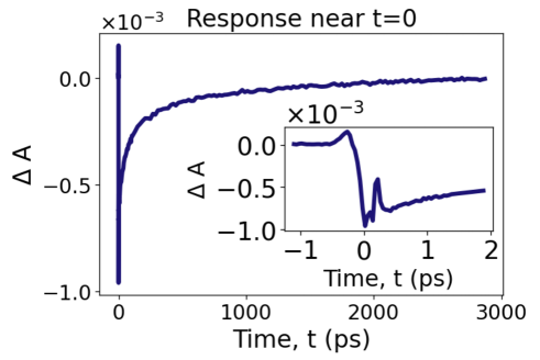
Figure S1: Transient absorption at 481 nm showing coherent, non-resonant response near $t=0$.

As we mentioned in the methods section that we excluded regions near $t=0$ for all analysis. Figure S1 shows transient absorption at $481$ nm. We see a response near $t=0$. Since, our specimen is a TiN nanoparticles in water, it is known that coherent, non-resonant response of the solvent can occur near $t=0$, hence we start our analysis from $t=0.78$ ps, avoiding this anomalous region.

Our initial data consists of 273 different wavelengths ranging from 421 nm to 743 nm, and each wavelength has $255$ absorption coefficients collected over time interval, $t=-5$ ps to $t=2870$ ps. The 421 nm to 431 nm wavelength data are excluded. The data is very noisy in this wavelength range due to the very small amount of continuum photons generated by 800 nm light incident on the sapphire crystal and very low levels of light in the probe beam causes large digitization noise in the measured signal. After excluding this anomalous region, we interpolate the data such that each wavelength has 256 absorption coefficients.

IX.2 (b) Ultrafast terahertz spectroscopy

Our initial data set consists of 26 and 151 scan along $\tau$ and $t$ respectively. As before, we preprocess the data and interpolate it to make $32\times 128$ for comparison among DCT, Haar and Hadamard. For the $\tau$ interval, we interpolate between the last two data points. For $t$ axis, we simply cutoff the data where the signal does not have any interesting feature. For the CS reconstruction, we randomly sample from $\tau$ and $t$. This corresponds to making a random coarse measurements in both $\tau$ and $t$ which significantly reduces the duration of experiment.

X Example of sampling for ultrafast terahertz spectroscopy

Here, we show an instance of what 15% sampling looks like. We can see that more samples are concentrated near $\tau=0$ because the time interval is very small compared to larger $\tau$ and lot more data is collected.

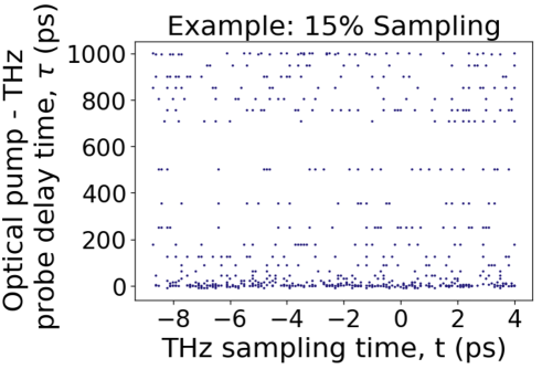
Figure S2: An instance of 15% sampling. Most of the samples are concentrated near $\tau=0$ because the time interval is very short compared to larger $\tau$.

XI Cross validation method for choosing $\lambda$

$\lambda$ is a free parameter which is data dependent. It is unknown beforehand what value of $\lambda$ to use for CS reconstruction. One approach to estimate $\lambda$ is by cross-validation which we use for both of our experimental data. For both experiments, we first randomly sample 20% of the full data. We use 80% of this sampled data for CS reconstruction and other 20% for cross validation. The method work as follows: we sweep over a range of $\lambda$ values and reconstruct the signal. Then, for each value of $\lambda$, we calculate the mean-square-error (MSE) between reconstructed signal and the other 20% data kept for cross validation. We then select the $\lambda$ value which gives the lowest MSE. For ultrafast transient absorption reconstruction, we chose the value of $\lambda$ that gives lowest MSE over all the wavelengths. Figure S3-a shows MSE as a function of $\lambda$ for ultrafast transient absorption. The value of $\lambda$ which gives minimum MSE is $8\times 10^{-5}$, and we used this value for CS analysis of ultrafast transient absorption spectroscopy. Similarly, Figure S3-b shows MSE as a function of $\lambda$ for ultrafast terahertz spectroscopy. The $\lambda$ value which minimizes the MSE is $2\times 10^{-4}$ and we used this value for all CS analysis of ultrafast terahertz spectroscopy.

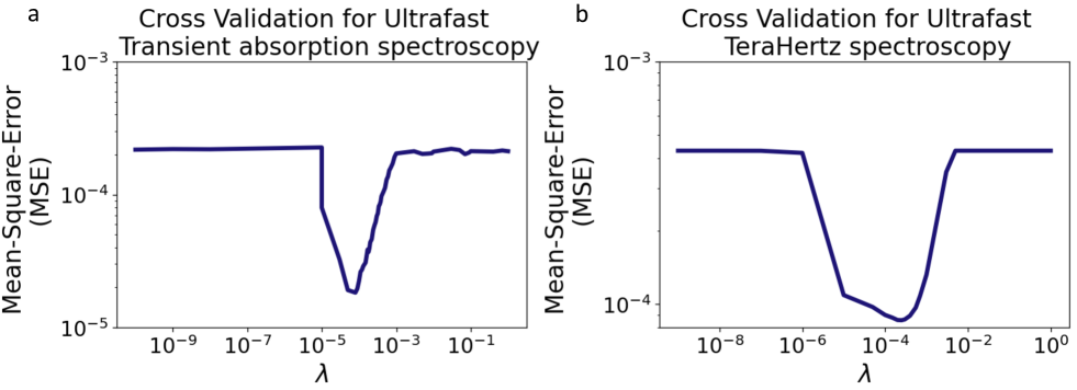
Figure S3: (a) Cross-validation for choosing $\lambda$ for ultrafast transient absorption spectroscopy. The minimum MSE is given by $\lambda=8\times 10^{-5}$. (b) Cross-validation for choosing $\lambda$ for ultrafast terahertz spectroscopy. The minimum MSE is given by $\lambda=2\times 10^{-4}$.

XII Assessing quality of CS reconstruction

To access the quality of CS reconstruction, we looks at how at the absolute difference between the CS reconstruction and the full experiment.

XII.1 (a) Ultrafast transient absorption spectroscopy

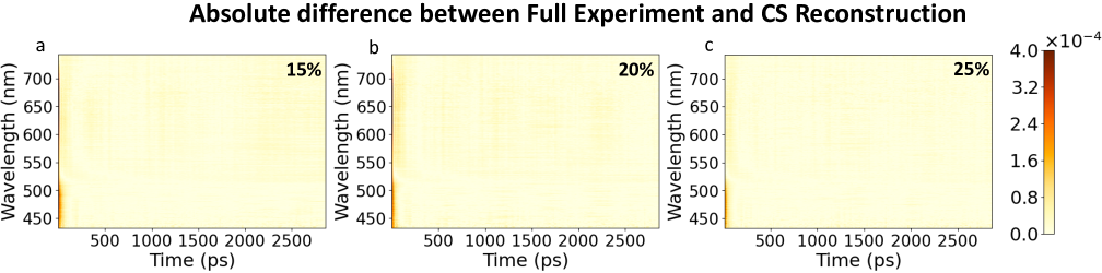
Figure S4: Figure shows the pixel-by-pixel magnitude difference between the full experiment and CS reconstructions at different sampling %.

XII.2 (b) Ultrafast terahertz spectroscopy

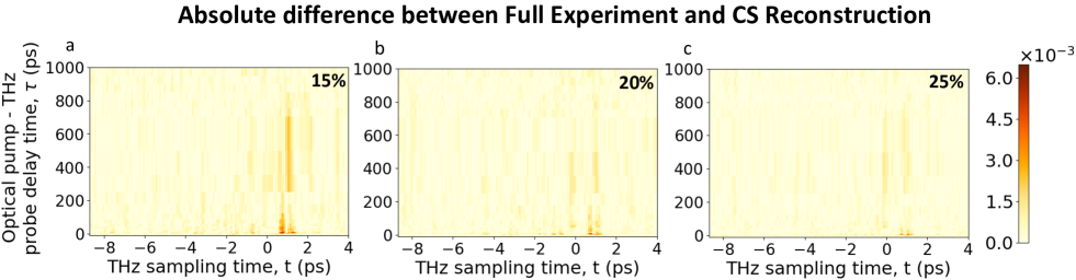
Figure S5: Figure shows the pixel-by-pixel magnitude difference between the full experiment and CS reconstructions at different sampling %.

XIII CS on another ultrafast terahertz spectroscopy experiment

We show another example of using CS in another ultrafast terahertz spectroscopy experiment. The specimen is a piece of silicon on an insulator (SOI) being optically pumped at about 650 nm near $\tau=0$ ps. We can see from Figure S6. that we can get fairly good estimate of the full experiment even with as low as 5% sample.

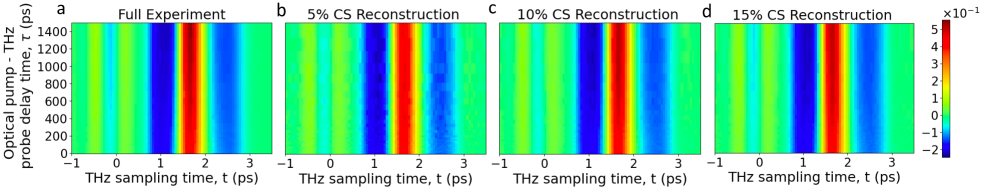
Figure S6: (a) shows the full experiment. (b), (c) and (d) shows the CS reconstruction with 5%, 10% and 15% samples, respectively

References

- Maiuri et al. (2019) Margherita Maiuri, Marco Garavelli, and Giulio Cerullo, “Ultrafast spectroscopy: state of the art and open challenges,” Journal of the American Chemical Society (2019).
- Hunt (2009) Neil T Hunt, “2d-ir spectroscopy: ultrafast insights into biomolecule structure and function,” Chemical Society Reviews 38, 1837–1848 (2009).
- Reid and Wynne (2006) Gavin D Reid and Klaas Wynne, “Ultrafast laser technology and spectroscopy,” Encyclopedia of Analytical Chemistry: Applications, Theory and Instrumentation (2006).
- Berera et al. (2009) Rudi Berera, Rienk van Grondelle, and John TM Kennis, “Ultrafast transient absorption spectroscopy: principles and application to photosynthetic systems,” Photosynthesis research 101, 105–118 (2009).
- Kraus et al. (2018) Peter M Kraus, Michael Zürch, Scott K Cushing, Daniel M Neumark, and Stephen R Leone, “The ultrafast x-ray spectroscopic revolution in chemical dynamics,” Nature Reviews Chemistry 2, 82–94 (2018).
- Shah (2013) Jagdeep Shah, Ultrafast spectroscopy of semiconductors and semiconductor nanostructures, Vol. 115 (Springer Science & Business Media, 2013).
- Weiner (2011) Andrew Weiner, Ultrafast optics, Vol. 72 (John Wiley & Sons, 2011).
- Guler et al. (2015) Urcan Guler, Sergey Suslov, Alexander V Kildishev, Alexandra Boltasseva, and Vladimir M Shalaev, “Colloidal plasmonic titanium nitride nanoparticles: properties and applications,” Nanophotonics 4, 269–276 (2015).
- Cortes et al. (2020) Cristian L Cortes, Sushovit Adhikari, Xuedan Ma, and Stephen K Gray, “Accelerating quantum optics experiments with statistical learning,” Applied Physics Letters 116, 184003 (2020).
- You et al. (2020) Chenglong You, Mario A Quiroz-Juárez, Aidan Lambert, Narayan Bhusal, Chao Dong, Armando Perez-Leija, Amir Javaid, Roberto de J León-Montiel, and Omar S Magaña-Loaiza, “Identification of light sources using machine learning,” Applied Physics Reviews 7, 021404 (2020).
- Kudyshev et al. (2019) Zhaxylyk A Kudyshev, Simeon Bogdanov, Theodor Isacsson, Alexander V Kildishev, Alexandra Boltasseva, and Vladimir M Shalaev, “Rapid classification of quantum sources enabled by machine learning,” arXiv preprint arXiv:1908.08577 (2019).
- Howland et al. (2011) Gregory A Howland, P Ben Dixon, and John C Howell, “Photon-counting compressive sensing laser radar for 3d imaging,” Applied optics 50, 5917–5920 (2011).
- Simmerman et al. (2020) E. M. Simmerman, H.-H. Lu, A. M. Weiner, and J. M. Lukens, “Efficient compressive and bayesian characterization of biphoton frequency spectra,” Opt. Lett. 45, 2886–2889 (2020).
- Baraniuk (2007a) Richard G Baraniuk, “Compressive sensing [lecture notes],” IEEE signal processing magazine 24, 118–121 (2007a).
- Candès and Wakin (2008) Emmanuel J Candès and Michael B Wakin, “An introduction to compressive sampling,” IEEE signal processing magazine 25, 21–30 (2008).
- Donoho (2006) David L Donoho, “Compressed sensing,” IEEE Transactions on information theory 52, 1289–1306 (2006).
- Candes et al. (2006) Emmanuel J Candes, Justin K Romberg, and Terence Tao, “Stable signal recovery from incomplete and inaccurate measurements,” Communications on Pure and Applied Mathematics: A Journal Issued by the Courant Institute of Mathematical Sciences 59, 1207–1223 (2006).
- Baraniuk (2007b) Richard G Baraniuk, “Compressive sensing [lecture notes],” IEEE signal processing magazine 24, 118–121 (2007b).
- Sun et al. (2016) Jian Sun, Huibin Li, Zongben Xu, et al., “Deep admm-net for compressive sensing mri,” in Advances in neural information processing systems (2016) pp. 10–18.
- Studer et al. (2012) Vincent Studer, Jérome Bobin, Makhlad Chahid, Hamed Shams Mousavi, Emmanuel Candes, and Maxime Dahan, “Compressive fluorescence microscopy for biological and hyperspectral imaging,” Proceedings of the National Academy of Sciences 109, E1679–E1687 (2012).
- Kazimierczuk and Orekhov (2011) Krzysztof Kazimierczuk and Vladislav Yu Orekhov, “Accelerated nmr spectroscopy by using compressed sensing,” Angewandte Chemie International Edition 50, 5556–5559 (2011).
- Howland and Howell (2013) Gregory A Howland and John C Howell, “Efficient high-dimensional entanglement imaging with a compressive-sensing double-pixel camera,” Physical review X 3, 011013 (2013).
- Katkovnik and Astola (2012) Vladimir Katkovnik and Jaakko Astola, “Compressive sensing computational ghost imaging,” JOSA A 29, 1556–1567 (2012).
- Shabani et al. (2011) A Shabani, RL Kosut, M Mohseni, H Rabitz, MA Broome, MP Almeida, A Fedrizzi, and AG White, “Efficient measurement of quantum dynamics via compressive sensing,” Physical review letters 106, 100401 (2011).
- Gross et al. (2010) David Gross, Yi-Kai Liu, Steven T Flammia, Stephen Becker, and Jens Eisert, “Quantum state tomography via compressed sensing,” Physical review letters 105, 150401 (2010).
- Zerom et al. (2011) Petros Zerom, Kam Wai Clifford Chan, John C Howell, and Robert W Boyd, “Entangled-photon compressive ghost imaging,” Physical Review A 84, 061804 (2011).
- Katz et al. (2009) Ori Katz, Yaron Bromberg, and Yaron Silberberg, “Compressive ghost imaging,” Applied Physics Letters 95, 131110 (2009).
- Wen et al. (2020) Xiewen Wen, Sushovit Adhikari, Cristian L. Cortes, David J. Gosztola, Stephen K. Gray, and Gary P. Wiederrecht, “Ghost imaging second harmonic generation microscopy,” Applied Physics Letters 116, 191101 (2020).
- Andrade et al. (2012) Xavier Andrade, Jacob N Sanders, and Alán Aspuru-Guzik, “Application of compressed sensing to the simulation of atomic systems,” Proceedings of the National Academy of Sciences 109, 13928–13933 (2012).
- Sanders et al. (2012) Jacob N Sanders, Semion K Saikin, Sarah Mostame, Xavier Andrade, Julia R Widom, Andrew H Marcus, and Alán Aspuru-Guzik, “Compressed sensing for multidimensional spectroscopy experiments,” The journal of physical chemistry letters 3, 2697–2702 (2012).
- Dunbar et al. (2013) Josef A Dunbar, Derek G Osborne, Jessica M Anna, and Kevin J Kubarych, “Accelerated 2d-ir using compressed sensing,” The Journal of Physical Chemistry Letters 4, 2489–2492 (2013).
- Cover and Thomas (2012) Thomas M Cover and Joy A Thomas, Elements of information theory (John Wiley & Sons, 2012).
- Soldevila et al. (2013) Fernando Soldevila, Esther Irles, V Durán, P Clemente, Mercedes Fernández-Alonso, Enrique Tajahuerce, and Jesús Lancis, “Single-pixel polarimetric imaging spectrometer by compressive sensing,” Applied Physics B 113, 551–558 (2013).
- Li (2010) Chengbo Li, An efficient algorithm for total variation regularization with applications to the single pixel camera and compressive sensing, Ph.D. thesis (2010).
- Wang et al. (2014) Lili Wang, Christopher McCleese, Anton Kovalsky, Yixin Zhao, and Clemens Burda, “Femtosecond time-resolved transient absorption spectroscopy of ch3nh3pbi3 perovskite films: evidence for passivation effect of pbi2,” Journal of the American Chemical Society 136, 12205–12208 (2014).
- Pendlebury et al. (2011) Stephanie R Pendlebury, Monica Barroso, Alexander J Cowan, Kevin Sivula, Junwang Tang, Michael Grätzel, David Klug, and James R Durrant, “Dynamics of photogenerated holes in nanocrystalline -fe 2 o 3 electrodes for water oxidation probed by transient absorption spectroscopy,” Chemical Communications 47, 716–718 (2011).
- Grancini et al. (2011) Giulia Grancini, Dario Polli, Daniele Fazzi, Juan Cabanillas-Gonzalez, Giulio Cerullo, and Guglielmo Lanzani, “Transient absorption imaging of p3ht: Pcbm photovoltaic blend: Evidence for interfacial charge transfer state,” The Journal of Physical Chemistry Letters 2, 1099–1105 (2011).
- Schmuttenmaer (2004) Charles A Schmuttenmaer, “Exploring dynamics in the far-infrared with terahertz spectroscopy,” Chemical reviews 104, 1759–1780 (2004).
- Luo et al. (2017) Liang Luo, Long Men, Zhaoyu Liu, Yaroslav Mudryk, Xin Zhao, Yongxin Yao, Joong M Park, Ruth Shinar, Joseph Shinar, Kai-Ming Ho, et al., “Ultrafast terahertz snapshots of excitonic rydberg states and electronic coherence in an organometal halide perovskite,” Nature communications 8, 1–8 (2017).
- Tibshirani (1996) Robert Tibshirani, “Regression shrinkage and selection via the lasso,” Journal of the Royal Statistical Society: Series B (Methodological) 58, 267–288 (1996).
- Chen et al. (2001) Scott Shaobing Chen, David L Donoho, and Michael A Saunders, “Atomic decomposition by basis pursuit,” SIAM review 43, 129–159 (2001).
- Lorenc et al. (2002) M Lorenc, M Ziolek, R Naskrecki, J Karolczak, J Kubicki, and A Maciejewski, “Artifacts in femtosecond transient absorption spectroscopy,” Applied Physics B 74, 19–27 (2002).
- Dietzek et al. (2006) Benjamin Dietzek, Torbjörn Pascher, Villy Sundström, and Arkady Yartsev, “Appearance of coherent artifact signals in femtosecond transient absorption spectroscopy in dependence on detector design,” Laser Physics Letters 4, 38 (2006).